SIMULATION OF ELECTRO-OSMOTIC FLOW INSIDE …me.bilkent.edu.tr/wp-content/uploads/2014/08/2011-ULIBTK-EOFLBM.pdf · INSIDE MICROCHANNELS USING LATTICE-BOLTZMANN METHOD ON GPUS Yi!it

ULIBTK’11 18. Ulusal Isı Bilimi ve Tekni!i Kongresi

07-10 Eylül 2011, ZONGULDAK

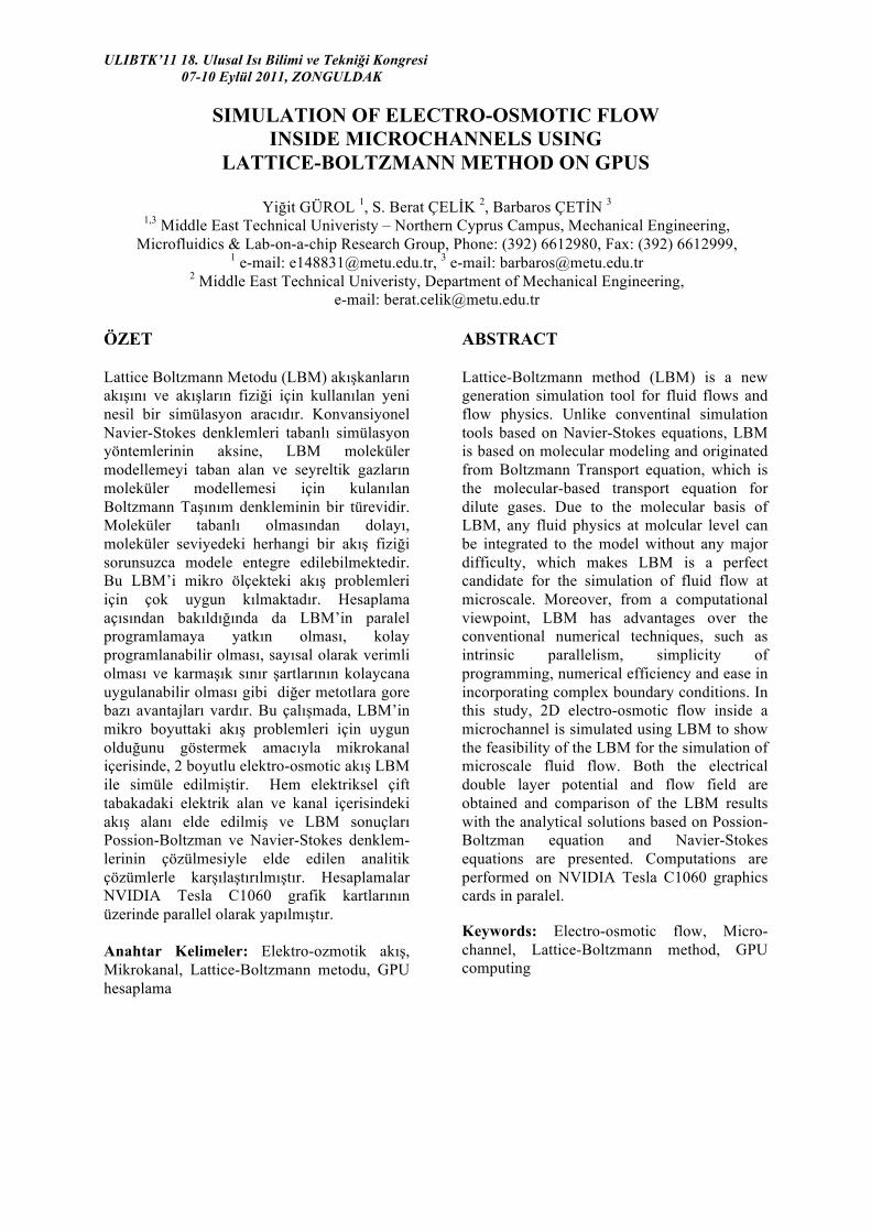
SIMULATION OF ELECTRO-OSMOTIC FLOW INSIDE MICROCHANNELS USING

LATTICE-BOLTZMANN METHOD ON GPUS

Yi!it GÜROL 1, S. Berat ÇEL"K 2, Barbaros ÇET"N 3 1,3 Middle East Technical Univeristy – Northern Cyprus Campus, Mechanical Engineering,

Microfluidics & Lab-on-a-chip Research Group, Phone: (392) 6612980, Fax: (392) 6612999, 1 e-mail: [email protected], 3 e-mail: [email protected]

2 Middle East Technical Univeristy, Department of Mechanical Engineering, e-mail: [email protected]

ÖZET Lattice Boltzmann Metodu (LBM) akı#kanların akı#ını ve akı#ların fizi!i için kullanılan yeni nesil bir simülasyon aracıdır. Konvansiyonel Navier-Stokes denklemleri tabanlı simülasyon yöntemlerinin aksine, LBM moleküler modellemeyi taban alan ve seyreltik gazların moleküler modellemesi için kulanılan Boltzmann Ta#ınım denkleminin bir türevidir. Moleküler tabanlı olmasından dolayı, moleküler seviyedeki herhangi bir akı# fizi!i sorunsuzca modele entegre edilebilmektedir. Bu LBM’i mikro ölçekteki akı# problemleri için çok uygun kılmaktadır. Hesaplama açısından bakıldı!ında da LBM’in paralel programlamaya yatkın olması, kolay programlanabilir olması, sayısal olarak verimli olması ve karma#ık sınır #artlarının kolaycana uygulanabilir olması gibi di!er metotlara gore bazı avantajları vardır. Bu çalı#mada, LBM’in mikro boyuttaki akı# problemleri için uygun oldu!unu göstermek amacıyla mikrokanal içerisinde, 2 boyutlu elektro-osmotic akı# LBM ile simüle edilmi#tir. Hem elektriksel çift tabakadaki elektrik alan ve kanal içerisindeki akı# alanı elde edilmi# ve LBM sonuçları Possion-Boltzman ve Navier-Stokes denklem-lerinin çözülmesiyle elde edilen analitik çözümlerle kar#ıla#tırılmı#tır. Hesaplamalar NVIDIA Tesla C1060 grafik kartlarının üzerinde parallel olarak yapılmı#tır. Anahtar Kelimeler: Elektro-ozmotik akı#, Mikrokanal, Lattice-Boltzmann metodu, GPU hesaplama

ABSTRACT Lattice-Boltzmann method (LBM) is a new generation simulation tool for fluid flows and flow physics. Unlike conventinal simulation tools based on Navier-Stokes equations, LBM is based on molecular modeling and originated from Boltzmann Transport equation, which is the molecular-based transport equation for dilute gases. Due to the molecular basis of LBM, any fluid physics at molcular level can be integrated to the model without any major difficulty, which makes LBM is a perfect candidate for the simulation of fluid flow at microscale. Moreover, from a computational viewpoint, LBM has advantages over the conventional numerical techniques, such as intrinsic parallelism, simplicity of programming, numerical efficiency and ease in incorporating complex boundary conditions. In this study, 2D electro-osmotic flow inside a microchannel is simulated using LBM to show the feasibility of the LBM for the simulation of microscale fluid flow. Both the electrical double layer potential and flow field are obtained and comparison of the LBM results with the analytical solutions based on Possion-Boltzman equation and Navier-Stokes equations are presented. Computations are performed on NVIDIA Tesla C1060 graphics cards in paralel. Keywords: Electro-osmotic flow, Micro-channel, Lattice-Boltzmann method, GPU computing



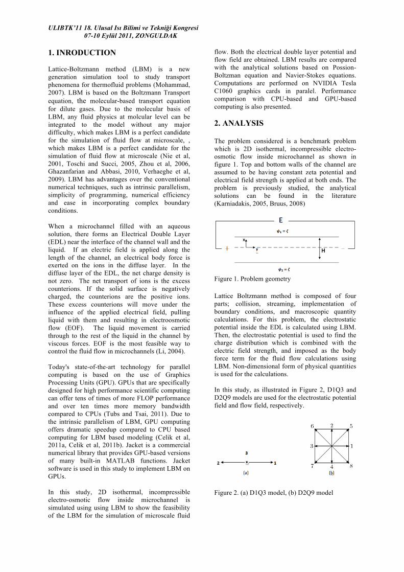
1. INRODUCTION Lattice-Boltzmann method (LBM) is a new generation simulation tool to study transport phenomena for thermofluid problems (Mohammad, 2007). LBM is based on the Boltzmann Transport equation, the molecular-based transport equation for dilute gases. Due to the molecular basis of LBM, any fluid physics at molcular level can be integrated to the model without any major difficulty, which makes LBM is a perfect candidate for the simulation of fluid flow at microscale, , which makes LBM is a perfect candidate for the simulation of fluid flow at microscale (Nie et al, 2001, Toschi and Succi, 2005, Zhou et al, 2006, Ghazanfarian and Abbasi, 2010, Verhaeghe et al, 2009). LBM has advantages over the conventional numerical techniques, such as intrinsic parallelism, simplicity of programming, numerical efficiency and ease in incorporating complex boundary conditions. When a microchannel filled with an aqueous solution, there forms an Electrical Double Layer (EDL) near the interface of the channel wall and the liquid. If an electric field is applied along the length of the channel, an electrical body force is exerted on the ions in the diffuse layer. In the diffuse layer of the EDL, the net charge density is not zero. The net transport of ions is the excess counterions. If the solid surface is negatively charged, the counterions are the positive ions. These excess counterions will move under the influence of the applied electrical field, pulling liquid with them and resulting in electroosmotic flow (EOF). The liquid movement is carried through to the rest of the liquid in the channel by viscous forces. EOF is the most feasible way to control the fluid flow in microchannels (Li, 2004). Today's state-of-the-art technology for parallel computing is based on the use of Graphics Processing Units (GPU). GPUs that are specifically designed for high performance scientific computing can offer tens of times of more FLOP performance and over ten times more memory bandwidth compared to CPUs (Tubs and Tsai, 2011). Due to the intrinsic parallelism of LBM, GPU computing offers dramatic speedup compared to CPU based computing for LBM based modeling (Celik et al, 2011a, Celik et al, 2011b). Jacket is a commercial numerical library that provides GPU-based versions of many built-in MATLAB functions. Jacket software is used in this study to implement LBM on GPUs. In this study, 2D isothermal, incompressible electro-osmotic flow inside microchannel is simulated using using LBM to show the feasibility of the LBM for the simulation of microscale fluid

flow. Both the electrical double layer potential and flow field are obtained. LBM results are compared with the analytical solutions based on Possion-Boltzman equation and Navier-Stokes equations. Computations are performed on NVIDIA Tesla C1060 graphics cards in paralel. Performance comparison with CPU-based and GPU-based computing is also presented.

2. ANALYSIS The problem considered is a benchmark problem which is 2D isothermal, incompressible electro-osmotic flow inside microchannel as shown in figure 1. Top and bottom walls of the channel are assumed to be having constant zeta potential and electrical field strength is applied at both ends. The problem is previously studied, the analytical solutions can be found in the literature (Karniadakis, 2005, Bruus, 2008)

Figure 1. Problem geometry

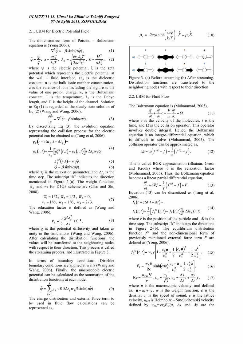
Lattice Boltzmann method is composed of four parts; collision, streaming, implementation of boundary conditions, and macroscopic quantity calculations. For this problem, the electrostatic potential inside the EDL is calculated using LBM. Then, the electrostatic potential is used to find the charge distribution which is combined with the electric field strength, and imposed as the body force term for the fluid flow calculations using LBM. Non-dimensional form of physical quantities is used for the calculations. In this study, as illustrated in Figure 2, D1Q3 and D2Q9 models are used for the electrostatic potential field and flow field, respectively.

Figure 2. (a) D1Q3 model, (b) D2Q9 model



2.1. LBM for Electric Potential Field The dimensionless form of Poisson – Boltzmann equation is (Yong 2006),

, (1)

, , , , (2)

where ! is the electric potential, " is the zeta potential which represents the electric potential at the wall – fluid interface, ##o is the dielectric constant, n is the bulk ionic number concentration, z is the valence of ions including the sign, e is the value of one proton charge, kb is the Boltzmann constant, T is the temperature, $d is the Debye length, and H is the height of the channel. Solution to Eq (1) is regarded as the steady state solution of Eq (2) (Wang and Wang, 2006),

, (3)

By discretizing Eq (3), the evolution equation representing the collision process for the electric potential can be obtained as (Tang et al, 2006).

(4)

, (5)

, (6) where !g is the relaxation parameter, and "tg is the time step. The subscript “k” indicates the direction mentioned in Figure 2-(a). The weight functions

and wk for D1Q3 scheme are (Chai and Shi,

2008), , , ,

, , , (7)

The relaxation factor is defined as (Wang and Wang, 2006),

, (8)

where % is the potential diffusivity and taken as unity in the simulations (Wang and Wang, 2006). After calculating the distribution functions, the values will be transferred to the neighboring nodes with respect to their direction. This process is called the streaming process, and illustrated in Figure 3.

In terms of boundary conditions, Dirichlet boundary conditions are applied at walls (Wang and Wang, 2006). Finally, the macroscopic electric potential can be calculated as the summation of the distribution functions at each node.

!

˜ " = gk + 0.5#tgwk$ sinh(% ˜ " )

k=1

3

& . (9)

The charge distribution and external force term to be used in fluid flow calculations can be represented as,

!

"e = #2ezn sinhez$

kbT

%

& '

(

) * , . (10)

Figure 3. (a) Before streaming (b) After streaming. Distribution functions are transferred to the neighboring nodes with respect to their direction 2.2. LBM for Fluid Flow The Boltzmann equation is (Mohammad, 2005),

, (11)

where c is the velocity of the molecules, t is the time, and & is the collision operator. This operator involves double integral. Hence, the Boltzmann equation is an integro-differential equation, which is difficult to solve (Mohammad, 2005). The collision operator can be approximated as,

!

" =# feq$ f( ) =

1

%feq$ f( ) , (12)

This is called BGK approximation (Bhatnar, Gross and Krook) where ' is the relaxation factor (Mohammad, 2005). Thus, the Boltzmann equation becomes a linear partial differential equation,

!

"f

"t+ c#f =

1

$feq% f( ) + F . (13)

Equation (13) can be discretized as (Tang et al, 2006),

(14)

where r is the position of the particle and "t is the time step. The subscript “k” indicates the directions in Figure 2-(b). The equilibrium distribution function f

eq and the non-dimensional form of previously mentioned external force term F are defined as (Yong, 2006),

, (15)

, (16)

, , , (17)

where u is the macroscopic velocity, and defined as, , w is the weight function, # is the density, cs is the speed of sound, c is the lattice velocity, uEO is Helmholtz – Smoluchowski velocity defined by uEO=$$oE%/µ, "x and "y are the



distances between nodes in x and y directions, respectively. The weight functions wk’s are

. (18)

The relaxation parameter is defined as,

, (19)

Streaming can be implemented as similar to the method represented in Figure 3, but as extended to 2D. For the boundary conditions, bounce-back boundary condition is implemented for the no-slip boundary condition at the walls, and periodic boundary conditions are used at the inlet and outlet (Wang and Wang, 2006). The summation of distribution functions at each lattice node represents the macroscopic fluid density. The momentum can be represented as an average of the lattice velocities, weighted by the distribution function (Chen and Doolen, 1998).

, (20)

Using Eq (20), macroscopic fluid density, (, and macroscopic velocity u can be calculated.

3. GPU IMPLEMENTATION As mentioned earlier, LBM offers simplicity of programming which results in a short and clean code (Çelik et al., 2011). Due to LBM’s intrinsic parallelism, it can be easily adapted to parallel computing. For this purpose, graphics cards are suitable as it has many embedded graphics processing units (GPUs) which can work simultaneously. In the past few years, NVIDIA has developed CUDA programming architecture to enable programmers to execute their codes on GPU. With this technology, execution times are considerably decreased to a level which cannot possibly be achieved using computational techniques on CPU (Accelereyes, 2011). LBM code is developed using MATLAB and ran serial on CPU (Intel Xeon E5620 Quad-Core 2.40GHz, 12MB Cache). To compare the results, the code ran parallel on GPU (Tesla C1060, 4GB RAM) using Accelereyes Jacket module for MATLAB.

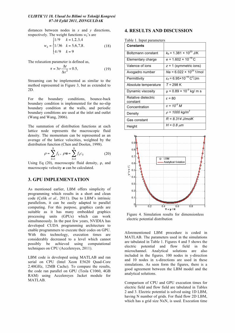
4. RESULTS AND DISCUSSION Table 1. Input parameters

Constants

Boltzmann constant kb = 1.381 ! 1023

J/K

Elementary charge e = 1.602 ! 10-19

C

Valence of ions z = 1 (symmetric ions)

Avogadro number Na = 6.022 ! 1023

1/mol

Permittivity !0 = 6.95!10-10

C2/Jm

Absolute temperature T = 298 K

Dynamic viscosity " = 0.89 ! 10-3

kg/ m s

Relative dielectric

constant ! = 80

Concentration c = 10-5

M

Density # = 1000 kg/m3

Gas constant R = 8.314 J/molK

Height H = 0.8 µm

Figure 4. Simulation results for dimensionless electric potential distribution

Aforementioned LBM procedure is coded in MATLAB. The parameters used in the simulations are tabulated in Table 1. Figures 4 and 5 shows the electric potential and flow field in the microchannel. Analytical solutions are also included in the figures. 100 nodes in y-direction and 10 nodes in x-directions are used in these simulations. As seen form the figures, there is a good agreement between the LBM model and the analytical solutions. Comparison of CPU and GPU execution times for electric field and flow field are tabulated in Tables 2 and 3. Electric potential is solved using 1D LBM, having N number of grids. For fluid flow 2D LBM, which has a grid size NxN, is used. Execution time



for each process is also given in tables in detail. As seen form the tables, GPU computing is faster than the CPU-based computing. For this grid size, in 1D model, much of time is spent in the boundary conditions step for CPU; however, much time is spent in the collision process in the GPU computation. For the 2D model, the share of the each process is more or less same for both CPU and GPU computations. As seen form Table 3, the main portion of the execution time is spent in the collision process for both computations. All four steps are faster, almost six times in GPU computation.

Figure 5. Simulation results for dimensionless velocity profile

To illustrate the effect of grid size on execution time, the code is run with different grid sizes. The results are tabulated in Table 4, and represented graphically in Figure 6. As can be seen clearly, for number of nodes less than 40000, executing the code on CPU is more effective. The reason for the slower execution time for small grid is that is that the amount of floating point operations resulting from coarse grids are not enough to keep the GPU busy. The major portion of the time is spent during the memory transfer to and from the GPU. As the grid gets finer, parallelization on the GPU becomes more and more effective, and with the increasing number of nodes, speedup increases, and GPU computing becomes advantageous. For the finest mesh of 256000 nodes; GPU computing offers 17 times of speedup compared to CPU. However, from the Figure 6, it can be concluded that, the increase in the number of nodes do not offer a dramatic speedup since the slope of the two lines are more or less same. However, use of multiple GPU cards for the GPU computation for the problems with larger scale (i.e. large 3D problems) may lead even higher speedup. Jacket library has also support for multiple GPUs. GPU computation with multiple GPUs will be our future research direction.

Table 2. Comparison of CPU and GPU execution time for electric potential field. (Grid size: 400).

Electric Potential Field

CPU (s)

% GPU (s)

%

Collision 0.0057 26.4 0.0210 59.3

Streaming 0.0072 33.3 0.0015 4.2

Boundary Conditions

0.0065 30.1 0.0044 12.4

Macroscopic Values

0.0022 10.2 0.0085 24.0

TOTAL 0.0216 100 0.0354 100

Table 3. Comparison of CPU and GPU execution time for flow field. 400x400 grid is used.

Flow Field CPU(s) % GPU(s) %

Collision 2.226 70.1 0.428 79.7

Streaming 0.171 5.4 0.028 5.2

Boundary Conditions

0.160 5.0 0.036 6.7

Macroscopic Values

0.620 19.5 0.045 8.4

TOTAL 3.177 100 0.537 100

Table 4. Comparison of CPU and GPU execution time (in seconds) for different grid size

Grid Size GPU Time

CPU Time

Speedup

60x60 2.43 1.10 0.45

80x80 2.44 1.41 0.58

100x100 2.44 1.58 0.65

150x150 2.45 2.33 0.95

200x200 2.46 3.57 1.45

300x300 2.46 6.16 2.51

400x400 2.49 9.62 3.86

600x600 2.76 17.6 6.38

800x800 3.12 30.4 9.74

1000x1000 3.60 44.7 12.4

1200x1200 4.36 60.9 14.0

1400x1400 5.18 81.6 15.8

1600x1600 6.11 105.0 17.2

Figure 6. Comparison of CPU and GPU execution time for different number of nodes



5. CONCLUSIONS In this study, the simulation of 2D electro-osmotic flow inside a microchannel using lattice Boltzmann method is presented. LBM shows excellent results in terms of accuracy, and due to the parallel programmability of LBM, GPU computing implementation significantly reduces the computation time. For number of nodes smaller than 40000, GPU computing is found to be slower than CPU. On the other hand, for larger number of nodes, GPU computing provides lower execution times, as it brings 17 times of speedup for 256000 nodes. However, for further increase in grid size, the speedup will remain constant. The use of Accelereyes JACKET module for MATLAB offers simplicity for coding as there exists built-in functions for specific purposes.

5. ACKNOWLEDGMENT Financial support from the METU–NCC via the Campus Research Project (BAP-FEN10) is greatly appreciated.

6. REFERENCES AccelerEyes. Getting Started Guide Jacket v1.7. 2011. Bruus H., Theoretical Microfluidics, Oxford

University Press, pp.148-159 2008. Chen S., Doolen G. D., Lattice Boltzmann Method for Fluid Flows, Annu. Rev. Fluid Mech. 30:329–64, 1998. Çelik, S. B., Sert, C., Çetin, B., Simulation of channel flow by parallel implementation of thermal Lattice-Boltzmann method on GPUs, 7th Internationl Conference on Computational Heat

and Mass Transfer (ICCHMT2011), July 18-22, 2011, Istanbul, Turkey. Çelik, S. B., Sert, C., Çetin, B., Simulation of lid-driven cavity flow by parallel implementation of Lattice-Boltzmann method on GPUs, 2nd Internationl Symposium on Computing in Science

and Engineering (ISCSE11), June 1-4, 2011, Turkey. Chai Z., Shi B., A novel lattice Boltzmann model for the Poisson equation, Applied! Mathematical

Modelling 32 2050–2058, 2008.

Ghazanfarian J., and Abbasi A., Heat transfer and fluid flow in microchannels and nanochannels at high Knudsen number using thermal Lattice-Boltzmann method. Phys. Rev. E. 82 (2): 026307, 2010. Karniadakis G., Beskok A., Aluru N., Microflows and Nanoflows: Fundamentals and Simulation,

Springer Science+Business Media, Inc., 2005. Li, D., Electrokinetics in Microfluidics, Elsevier

Academic Press, 1-150, 2004. Mohammad, A. A., Applied Lattice Boltzmann Method for Transport Phenomena, Momentum, Heat and Mass Transfer. Sure Printing, Calgary,

2007. Nie X., Doolen G. D., and Chen S., Lattice-Boltzmann simulation of fluid flows. MEMS J. of

Statistical Phys. 107 (1-2): 279-289, 2001. Succi, S., The Lattice Boltzmann Equation for Fluid Dynamics and Beyond. Oxford University Press,

New York, 2001. Tang G. H., Li Z., Wang J. K., He Y. L. and Tao W. Q., Electroosmotic flow and mixing in microchannels with the lattice Boltzmann method, Journal of Applied Physics, 100, 094908, 2006. Toschi F. and Succi S., Lattice Boltzmann method at finite Knudsen numbers. Europhys. Lett 69(4): 549-555, 2005. Verhaeghe F., Luo L.-S., and Blanpain B. Lattice Boltzmann modeling of microchannel flow in slip flow regime. Journal of Computational

Physics. 228 (1): 147-157, 2009. Wang J., Wang M., Lattice Poisson-Boltzmann Simulations of Electro-osmotic Flows in Microchannels, Journal of Colloid and Interface

Science. 296(2): 729-736, 2006.!!

Yong S., Lattice Boltzmann models for microscale flows and heat transfer, Ph.D Dissertation, Hong-

Kong University of Science and Technology, 2006.

Zhou Y., Zhang R., Staroselsky I., Chen H., Kim W. T., and Jhon M. S., Simulation of micro and nano scale flows via the Lattice Boltzmann method. 362 (1): 68-77, 2006.

Documents

SIMULATION OF ELECTRO-OSMOTIC FLOW INSIDE …me.bilkent.edu.tr/wp-content/uploads/2014/08/2011-ULIBTK-EOFLBM.pdf · INSIDE MICROCHANNELS USING LATTICE-BOLTZMANN METHOD ON GPUS Yi!it