doi.org/10.26434/chemrxiv.12221477.v1

Simulation of Excitation by Sunlight in Mixed Quantum-ClassicalDynamicsMario Barbatti

Submitted date: 30/04/2020 • Posted date: 04/05/2020Licence: CC BY-NC-ND 4.0Citation information: Barbatti, Mario (2020): Simulation of Excitation by Sunlight in Mixed Quantum-ClassicalDynamics. ChemRxiv. Preprint. https://doi.org/10.26434/chemrxiv.12221477.v1

This paper proposes a method to simulate nonadiabatic dynamics initiated by thermal light, including solarradiation, in the frame of mixed quantum-classical (MQC) methods, like surface hopping. The method isbased on the Chenu-Brumer approach, which treats the thermal radiation as an ensemble of coherent pulses.It is composed of three steps, 1) sampling initial conditions from a broad blackbody spectrum, 2) propagationof the dynamics using conventional methods, and 3) ensemble averaging considering the field and realizationtime of the pulses. The application of MQC dynamics with pulse ensemble (MQC-PE) to a model system ofnucleic acid photophysics showed the emergence of a stationary excited-state population. In another testcase, modeling retinal isomerization, MQC-PE revealed that even when the underlying photophysics occurswithin 200 fs, it may take tens of microseconds of continuous solar irradiation to activate a moleculephotochemically. Such emergent long timescales may impact our understanding of biological andtechnological phenomena occurring under solar radiation.

File list (2)

download fileview on ChemRxivmanuscript.pdf (708.69 KiB)

download fileview on ChemRxivsupporting_info.pdf (490.81 KiB)

1

Simulation of Excitation by Sunlight in

Mixed Quantum-Classical Dynamics

Mario Barbatti

Aix Marseille University, CNRS, ICR, Marseille, France

mario.barbatti@univ-amu.fr – www.barbatti.org

Abstract

This paper proposes a method to simulate nonadiabatic dynamics initiated by thermal light,

including solar radiation, in the frame of mixed quantum-classical (MQC) methods, like surface

hopping. The method is based on the Chenu-Brumer approach, which treats the thermal radiation

as an ensemble of coherent pulses. It is composed of three steps, 1) sampling initial conditions

from a broad blackbody spectrum, 2) propagation of the dynamics using conventional methods,

and 3) ensemble averaging considering the field and realization time of the pulses. The application

of MQC dynamics with pulse ensemble (MQC-PE) to a model system of nucleic acid photophysics

showed the emergence of a stationary excited-state population. In another test case, modeling

retinal isomerization, MQC-PE revealed that even when the underlying photophysics occurs

within 200 fs, it may take tens of microseconds of continuous solar irradiation to activate a

molecule photochemically. Such emergent long timescales may impact our understanding of

biological and technological phenomena occurring under solar radiation.

2

I. Introduction

Nonadiabatic mixed quantum-classical (NA-MQC) dynamics encompass some of the most

popular methods to simulate nonadiabatic molecular dynamics after a photoexcitation.1-3 In these

methods, the nuclear motion follows classical equations, while electrons are treated quantum-

mechanically. The equations-of-motion are complemented by nonadiabatic algorithms, allowing

to couple different electronic states. The advantage of such methods is that they allow to retain full

dimensionality and do not require pre-computed or parametrized potential energy surfaces.

NA-MQC simulations are usually set to be compared to experimental data from time-

resolved spectroscopy, where the molecular systems are excited by coherent ultrashort sub-100-fs

pulses, pumping the molecular systems into specific bands.4 Despite several developments aiming

at dealing with the initial laser field acting on the molecule,5-12 most simulations just assume

instantaneous pulses, with the molecule starting its dynamics in one or few excited states of a

single absorption band. (For a recent discussion on this issue, including the proposition of a new

approach to sample continuum-wave (CW) fields, see Ref.13)

To the best of my knowledge, one aspect that has not been discussed in the context of NA-

MQC dynamics is how to simulate excitation by thermal radiation, most specifically sunlight.

Brumer and co-workers have pioneered in the studies of photochemistry induced by thermal light,

using different methodologies.14-17 In addition to the expected broadening of the spectral excitation

range, they have shown that thermal light should kill all time-dependent coherences commonly

observed in the results of ultrafast spectroscopy.17 Moreover, the continuous field slowly populates

the excited states, giving rise to long time constants sometimes exceeding milliseconds, even when

the underlying photophysics is within the picosecond regime.14 Therefore, to master the

methodologies to simulate the molecular response to thermal light may profoundly impact the way

3

we investigate many different fields, including photosynthesis, vision, solar-induced mutagenesis

and carcinogenesis, photovoltaic devices, environmental and atmospheric photochemistry to name

a few.

How should we translate such a broad-brand, incoherent, continuous radiation acting on a

molecule into NA-MQC trajectories? Should each trajectory be created in a coherent superposition

of excitations covering the spectral radiation? Should the excitation be treated incoherently, with

each trajectory created in a different state of the spectrum? Should the trajectories be necessarily

propagated with the molecule under a stationary electric field?

In this paper, I address these questions by adapting the transform-limited-pulse

representation of thermal light proposed by Chenu and Brumer.15 This approach is particularly

well-suited to be used in NA-MQC dynamics because the incoherent radiation is treated as an

ensemble of coherent pulses, providing a natural bridge for methods like surface hopping.

Assuming the validity of the first-order perturbation theory of radiation-matter interaction

in a stationary field of a black body at temperature T, Chenu and Brumer15 have shown that the

thermal light can be described as an ensemble average of realizations of coherent pulses. Each

field realization is a pulse given as

( ) ( ) ( )3

/3 3

0 0

,4 1B

i ts

k T

t AE t d e

c e

− −

=− (1)

where ts is an arbitrary timescale constant, A is an attenuation factor discussed later, and marks

the time of each realization of the pulse. In the case of the sunlight, with a temperature T = 5778

K,18 the pulse described by Eq. (1) has about 5 fs duration and a peak amplitude of 1 kV/m, as

shown in Fig. 1.

4

Fig. 1 Pulse shape for the field realization at = 0. The shape for the other field realizations is the

same but displaced in time.

In practical terms, in the Chenu-Brumer approach, the thermal excitation happens over an

ensemble of molecules, each of them excited by a different realization of ( ) ( )E t . Thus, can be

interpreted as a counting index of the ensemble. It must be emphasized that the excitation process

must always be described by an average over the ensemble, while a single realization does not bear

any physical meaning in itself.

Such an ensemble of short coherent pulses has a familiar ring for users of NA-MQC

methods. These methods are naturally tailored to work with ensembles, in the form of either

independent or coupled trajectories.19-21 The results from surface hopping,21 in particular, also only

make sense as an average over the ensemble. Moreover, the ultrashort pulse of each realization

plays favorably for the validity of the instantaneous approximation.

Therefore, it seems natural to identify each pulse realization to a different trajectory in the

NA-MQC simulations, using them to define a set of initial conditions to start dynamics. There is

a catch, however: a coherent pulse as short as 5 fs must cover a broad spectral band, and as such,

5

it poses a challenge to define the initial electronic states. I show below that there are different ways

of dealing with this issue, depending on the NA-MQC method adopted. After having defined the

broadband initial conditions for dynamics, we can run the simulations in conventional ways, thanks

to the short pulses. Finally, the results of the dynamics must be averaged accounting for the effect

of the weak pulse on the electronic density and the fact that each pulse occurs at a different time.

I call all this three-step procedure NA-MQC dynamics with pulse ensemble (MQC-PE). Before

discussing it, however, we should first review some key points of the Chenu-Brumer approach.

II. The Chenu-Brumer approach for thermal light

Each pulse realization (Eq. (1)) excites the molecule into an electronic wavepacket given

by

( ) ( ) ( ) ' /

' '

' 1

, ' ,N

i t

s gt K t A C t e

−

=

= (2)

where ' counts over the N electronic excited states of the molecule. For a specific state , with

wavefunction , the energy is and transition dipole moment norm is g. K and C are

2 3

0

9

64K i

c = − (3)

and

( ) ( ) ( ) ( )

( )( ) ( )( )

, ,

0

3/2

12

, 1 , 0,23

8, 0, ,

3

g

j

j j

j

i t

g g j g j

C t i J t J

j

i e F h t F h

=

− = − −

− −

(4)

6

where ( ) /g g = − ,

( )( )

( )

( ) ( )

, 3/2

2 , 1, ,

,

1, ,

2

gi g j

j

j

j

B

h tJ t e

h t

h t j i tk T

+=

= + + −

(5)

and ( )F x is the Dawson function

( )2 2

0

.

x

x yF x e e dy− (6)

The definition of K in Eq. (3) differs from that in the original paper by a factor 3 . This factor

stems from the missing sum over of three cartesian coordinates of the electric field of the thermal

light in Eq. (7) of Ref. 15 (see Supporting Information (SI), note SI-1).

In practical terms, the infinite sum in Eq. (4) is replaced by a finite sum over the first N

terms, ( )N

C C . As shown in Figure SI-1, only few terms are needed to reach convergence.

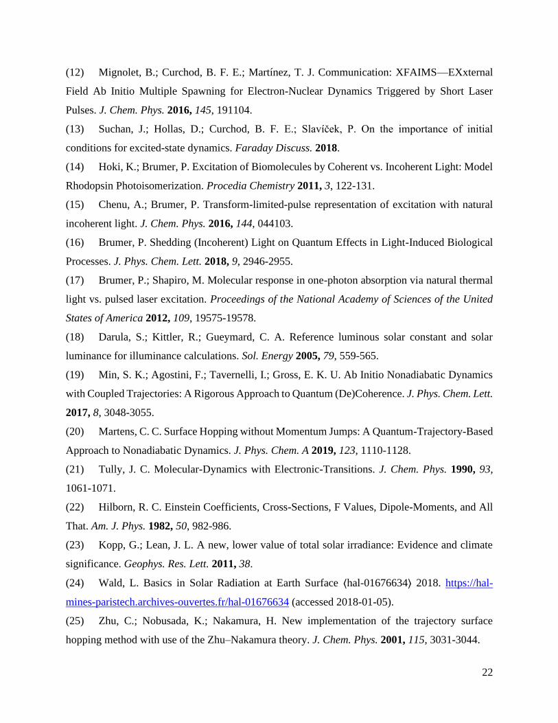
After the pulse is over, the coefficients tend to a constant value (Fig. SI-2), which is a

function of the excitation energy /g g = of state (Fig. SI-3). A significant feature is that

( )2

,C does not depend on for values larger than 5 fs (Fig. 2), as it becomes proportional to

the spectral radiance of the black body

( )3

2

/, .

1g B

g

k TC

e

− (7)

7

Fig. 2 ( ) ( )2

,N

C t as a function of the energy of state , plotted for different values of . Values

computed for t = 10,000 fs and N = 4. The blackbody spectral radiance at T = 5778 K is the solid

line underlying the curves for large values. It has been normalized by maximum of the curve for

= 5 fs.

For a single realization , the population in state at time t is given by

( ) ( ) ( ) ( )

( )

2

2 22, ,s g

t t

K t A C t

=

=

(8)

and the coherence between excited states and is

( ) ( ) ( ) ( ) ( ) ( )

( ) ( )2 * /* , , ,

i t

s g g

t t t

K t A C t C t e

−

=

= (9)

where = − is the energy gap between the states. ( )2

,C t and ( ) ( )*

, ,C t C t are shown

in Fig. SI-4. Note that the density matrix elements ( ) ( )t

are given per unit of area.

After the field is over, the population of state is

8

( ) ( ) ( )2

2

2 3

0

27, .

128

g

s

e g

fet A C

m c

= (10)

For convenience, the transition dipole moment was rewritten in terms of the oscillator strength fg

using22

2

2 3.

2

g

g

e g

fe

m

= (11)

Eq. (10) shows that the probability of exciting state is proportional to the product of a

molecular factor /g gf and a field factor ( )2

,C accounting for the spectral distribution.

( )2

,C modulates the probabilities, enhancing molecular transitions in the red-to-blue region

(1.5 to 2.5 eV). For values near zero, the modulation is broader, from infrared to violet (see Fig.

2).

Any quantity derived from the Chenu-Brumer approach must be analyzed in terms of an

ensemble average, which for the density matrix elements is given as

( ) ( ) ( )

( ) ( )1

0

1

1,

tot

s

N

ks

t d tt

tt

−

−

=

=

(12)

where is the time interval between consecutive field realizations and N is the total number

of realizations. In the ensemble average, ts cancels out (it also appears within ( ) ( )t

), and because

of that, it does not impact the averaged results. However, quantities relative to each field realization

are still dependent on ts, and it is desirable to attribute a reasonable value to it. Given the definition

of the ensemble average in Chenu-Brumer approach, ts should be the time interval between

consecutive field realizations .

9

The original derivation of the Chenu-Brumer approach is strictly valid near the surface of

the black body generating the thermal light (equivalent to A = 1 in all previous equations). To

simulate sunlight reaching our planet, we should consider that the orbital distance attenuates the

emitted power. Thus, if the Sun's radius is RS and the Earth-Sun distance is D, the attenuation factor

is

2

2.SR

AD

= (13)

With such attenuation factor and ts = 1 fs, the electric field pulse in Eq. (1) has a peak intensity of

( ) ( )2

0 2

0

10 1542 W/m

2PI c E= = , slightly above the mean annual solar irradiance at the top of

the atmosphere, 1361 W/m2.23 The factor A should be further reduced by about 25% to match the

solar irradiance at Earth's surface, about 1000 W/m2. Nevertheless, an accurate description of the

solar radiation at the surface should also consider the spectral deviation from the blackbody profile

caused by diverse atmospheric factors.24

III. NA-MQC dynamics with pulse ensemble (MQC-PE)

To simulate the thermal light in MQC-PE, we should 1) create an ensemble of initial

conditions for trajectories, each one corresponding to a single field realization, 2) run the dynamics

for each trajectory, and 3) do a statistical analysis of the ensemble. The first step should consider

the broad-spectrum excitation. The second step is nonadiabatic dynamics as usual. The third step

should consider that each realization happens at a different time and that the excitation probability

depends on the field. Let us discuss in more detail each of these steps.

In Ehrenfest dynamics2 and fewest switches surface hopping,21 nonadiabatic information

is computed from the ( )t coefficients of the time-dependent wavefunction

10

( ) ( )'

' 1

' .N

t t

=

= (14)

In the simulations, ( )0 is usually assumed to be the unity at the initially occupied state and null

in the others. Comparing this equation to Eq. (2), we could alternatively assign the coefficients of

each state to the Chenu-Brumer coefficient for each trajectory.

If the NA-MQC method includes electric-field propagation,5-12 the wavefunction can be

initialized with

( ) ( )0 0, ,s gt K t As C = = (15)

and the field in Eq. (1) should be included in the Hamiltonian. In this equation, s is the area of the

molecule exposed to the radiation.

On the other hand, if the NA-MQC method does not include electric field propagation (as

usually it is the case), we may use the Chenu-Brumer coefficients after the field is over to initialize

the electronic wavefunction:

( ) ( )0 , .s gt K t As C = = (16)

Such prescription may work well for Ehrenfest dynamics, in which the trajectory is propagated in

the weighted mean of the potential energy surfaces of the electronic states. It can also be used to

initialize the wavefunction coefficients in fewest switches surface hopping. Nevertheless, in this

case, the use of Eq. (16) is not fully consistent, as the classical equations for the nuclei would still

be initialized in a single state. Either way, Eq. (16) creates an initially coherent wavefunction for

each trajectory (we may call it coherent initial conditions, or CIC).

11

Another possibility for using the Chenu-Brumer approach for simulating thermal light

excitation in MQC dynamics without electric-field propagation is just to sample a number of

trajectories starting in each state proportional to ( )P

, which is defined in terms of the population

(Eq. (10)) as

( )

( ) ( )

( ) ( )' '

' 1

.N

P

=

=

(17)

Such prescription should also be valid beyond the fewest switches approach, for surface hopping

variants that do not explicitly propagate the electronic coefficients, like the Zhu-Nakamura

method.25 Different from the CIC approach, using ( )P

to sample the initial states creates an

entirely incoherent ensemble of initial conditions (IIC).

Both the coherent and the incoherent approaches for initial conditions for dynamics without

field propagation assume that the pulse is instantaneous, in the sense that there is no nuclear motion

during the field application. This is a reasonable hypothesis in the case of the sunlight, with pulses

shorter than 5 fs (see Fig. 1), as the fastest motions in ordinary molecules are X-H stretching

modes, with periods of about 10 fs. Nevertheless, cold blackbody sources may be completely out

of the scope of the method. To give an extreme example, the microwave background produced at

2.7 K has pulses lasting 5 ps,15 therefore, intermixing with the molecular dynamics.

After generating the initial conditions, the dynamics simulations are not different from the

usual. An instantaneous pulse initiates the molecular excitation, and we propagate the state

evolution afterward. This process is repeated for an ensemble of N trajectories.

12

Any quantity computed as a function of time for each trajectory must be analyzed in the

ensemble average. Making use of Eq. (12), the ensemble average of a quantity ( ) ( )Q t is

( ) ( ) ( ) ( ) ( )1

0

1,

Nk t ktot

ks

Q t Q tt

−

=

= (18)

where is the initial state and ( )kQ

means that the initial time for the corresponding trajectory

should be shifted to 0t k = . Here ( )totQ t is given per unit of area. It should be multiplied by s

to get it per molecule.

IV. Test cases

Let us first discuss the broadening of the excitation spectrum. Fig. 3-a shows the absorption

cross-section of 9H-adenine as a function of the excitation energy. It was computed as a simple

Gaussian convolution26 of vertical excitation energies and oscillator strengths for 40 adiabatic

states. These states were calculated in the gas phase with the resolution-of-identity algebraic

diagrammatic construction to second order27-28 (RI-ADC(2)) using the aug-cc-pVDZ basis set.29

The convolution was done assuming 0.3 eV bandwidth and 0.1 eV shift for all transitions. Fig. 3-

top also shows the probability ( )

P

(Eq. (17)) calculated at = 0 and 3 fs. The probability

distributions for larger than 3 fs are virtually identical to the 3-fs curve.

13

Fig. 3 Top: absorption cross-section and excitation probabilities as a function of the excitation

energy (Eq. (17)) for adenine. The probability curves were normalized by the maximum of the first

cross-section band. Bottom: Excitation probability (( )3

P ) of each adiabatic state S.

From the molecular properties only, without considering the solar radiation, the cross-

section shows three strong bands at 5.0, 6.5, and 7.5 eV. Nevertheless, when the solar radiation is

considered, excitation in the high-energy bands is screened out. For the first field realization at

= 0 fs, the probability of exciting the strongest band at 6.5 eV is reduced to approximately the same

as to excite the first band. For the following field realizations, this probability becomes even

smaller, although still sizable. For a large number of field realizations, it is statistically safe to

neglect the odd behavior of ( )0

P , and take ( )3

P

(dashed curve in Fig. 3-top) to sample the initial

state for all starting trajectories. For instance, taking the minimum of the ground-state geometry,

14

the probability ( )3P associated with each of the 40 adiabatic states is plotted in Fig. 3-bottom.

Following this distribution, for a set of 100 trajectories, we should start 59 in state S2, 16 in state

S10, 7 in state S3, 4 in S1, 3 in S11, and so on.

If the initial conditions are formed by an ensemble of geometries spanning the phase space

(via a Wigner distribution, for instance30), the initial state for a specific geometry should be

assigned by ( )3P computed for that geometry. In this example of adenine, it would imply that most

of the trajectories would start in the states forming the first band, a considerable number of

trajectories would begin in the states forming the second band, and some few trajectories would

start in the states forming the third band. Such distribution of initial states is strikingly distinct

from what we do when simulating monochromatic radiation, in which a single state is initially

populated, usually within a narrow excitation energy window.31

To illustrate the role of the ensemble average, I will discuss two analytical models

emulating some typical nonadiabatic MCQ dynamics results (Fig. 4). I start with a model for DNA

photophysics.32 We assume that each nucleotide can be initially photoexcited with any energy

within a Gaussian absorption band centered at 4.77 eV and with a standard deviation of 0.3 eV.

The band has oscillator strength 1. (Note that I am neglecting the excitation into the high energy

bands.) After an instantaneous excitation, the nucleotide is supposed to return to the ground state

with 1 ps lifetime (Fig. 4-a).33 (I am also neglecting long-lived excitation processes.34) Suppose

we have run nonadiabatic dynamics, say with surface hopping, and we are monitoring the current

molecular state. We define the function i(t) that has value 0 when the molecule is in the ground

state and 1 when it is in the excited state. Considering that each trajectory starts at a different time

, the excited-state population of a single trajectory as a function of the time can be modeled as

15

( ) ( ) ( )( )0, ,ri t t H t H t t = = − − − + (19)

where H(t) is the Heaviside function, and tr is the internal conversion time sampled from an

exponential distribution with 1 ps time constant.

Fig. 4 Analytical models emulating results from MQCD trajectories. (a) DNA model (Eq. (19)).

Trajectories are excited at the time and return to the ground state at + . Each trajectory starts

at a different . (b) Function ( )toti t (Eq. (20)) telling the excited-state population of nucleobases

as a function of time. (c) Retinal model with two types of trajectories starting at the time (Eq.

(21)). The solid curve illustrates a trajectory that isomerizes at time . The dashed curve represents

a trajectory that does not isomerize. 65% of trajectories are of the first type. (d) ( )toti t for the

population of the trans photoisomer. The inset shows ( )toti t for N = 10 and 20 thousand. In both

models, is sampled from a statistical distribution.

16

Using Eq. (18), the ensemble-averaged excited-state population (per unit of area) is

( ) ( ) ( ) ( ) ( )1

0

1.

Nk t ktot

ks

i t i tt

−

=

= (20)

This quantity is plotted in Fig. 4-b for N equal to 10,000 and 20,000 trajectories, each trajectory

corresponding to one field realization. is 1 fs and, as discussed, ts = . The figure shows that

the ensemble-averaged excited-state population increases as a function of time nearly independent

of N. Initially, there is a fast, transient rise triggered by the field starting at time 0. At 3 ps, the

population reaches a stationary regime and remains constant while each excitation is compensated

by a return to the ground state. After the illumination window is closed at N , the excited-state

population quickly drops. The mean value of the excited-state population in the stationary region

is tot

meani = 1.8×10-11 Å-2.

To get a feeling of the impact of this density, consider that a human skin cell has Nnuc =

6.4×109 nucleotides.35 If the nucleobase area exposed to the radiation is s = 17 Å2 (see Fig. SI-5),

it means that under continuous solar irradiation, there are always about 2tot

nuc meanN i s = excited

nucleotides in the cell.

As a second example, consider the cis-trans photoisomerization of retinal.36 In this case,

the molecule is supposed to be initially in the cis isomer, and only one excited state is considered,

with excitation energy 2.1 eV and oscillator strength 1. After an instantaneous excitation, the

molecule may isomerize into trans following an exponential distribution within 200 fs time

constant and 0.65 quantum yield. Once more, suppose we have run surface hopping, and we are

monitoring the molecular isomer at each time step of each trajectory. We define the function i(t)

that returns 0 when the molecule is in the original conformation (cis) or 1 if the new isomer (trans)

17

is formed (Fig. 4-c). To compute the ensemble average, we should consider that each trajectory

starts at a different time . Under these conditions, the isomeric form at time t for a single trajectory

can be modeled as

( ) ( )( )0, ,r yi t t H t t r = = − + (21)

where tr is the isomerization time sampled from an exponential distribution with 200 fs time

constant, and ry is a random number sampled from a Bernoulli distribution with probability 0.65.

By construction, 35% of trajectories will be at i(t) = 0 at all times.

The function ( )toti t can be computed in the same way as in Eq. (20). Fig. 4-d shows that

the ensemble-averaged trans population increases as a function of time. In the first 200 fs there is

a transient due to the first field realization at time 0. After that, the population increases at a

constant rate, which is approximately independent of N. Finally, after the illumination window is

closed at N the population starts to saturate at different levels depending on N. In principle,

while the light is shining and the cis population is not depleted, the trans population should

continue to raise with a constant rate. Fitting the region of linear rise of ( )toti t with a linear function

gives a rate of ktrans = 4.3×1022 s-1m-2 for the trans isomer formation. Taking the cis-retinal area as

s = 56 Å2 (Fig. SI-5), the rate per molecule is 4 -12.4 10 ss transk k s= = . This means it takes 42 s

of continuous solar irradiation to isomerize the molecule. The ks rate calculated under other

illumination conditions is given in Table 1.

Considering that a cone cell has about Nret = 7.8×107 retinal molecules,37 how long should

the cell be irradiated before the isomerization starts? The probability per cone cell that r or more

of these molecules will be in the trans conformation at time t follows the binomial distribution14

18

( ) ( ) ( )1

0

1 1 ,ret

s s

ri N i

ret k t k tr

trans s s

i

Np t k te k te

i

−−

− −

=

= − −

(22)

where sk t

sk te− is the Poisson probability of isomerization of a single molecule at time t. Therefore,

under continuous solar irradiation, it takes about 0.5 ps to isomerize one or more molecules and 6

ps to isomerize more than ten molecules.

Table 1 Cis-trans isomerization rate per molecule under different illumination conditions.

Computed with MQC-PE with the retinal model (Eq. (21)) and s = 56 Å2 unless stated otherwise.

Condition T (K) A ( 2 2/SR D ) ks (s-1)

Extra-terrestrial 5778 1 2.4×104

Ground level 5778 0.75 1.8×104

Scotopic vision 4100 3.06×10-11 1.2×10-7 (MQC-PE)

1.9×10-7 (Redfield theory14)

Hoki and Brumer14 studied retinal isomerization under incoherent light excitation using the

Redfield theory applied to a one-dimensional model coupled to a bath. They showed that under

conditions of scotopic vision (T = 4100 K and maximum luminance 0.06 cd.m2), the cis-trans

isomerization rate is 1.9×10-7 s-1 (Table 1), corresponding to about 1.3 ms of continuous irradiation

to isomerize one or more molecules in a rod cell containing 4×109 retinal molecules. With MQC-

PE (see note SI-2), the isomerization rate under the same condition is 1.2×10-7 s-1, and it takes 1.9

ms to isomerize one or more molecules in a rod cell. The excellent agreement between these two

completely distinct approaches is a good indication of the validity of the MQC-PE method.

In both examples discussed here, I showed results for up to N = 20,000 trajectories (or

field realizations). This is a large number viable only for analytical models. If our goal in MQC-

PE is to run realistic situations, where trajectories are computed with on-the-fly electronic structure

19

calculations, the affordable number of trajectories is one hundred times smaller, about 200. This

means that each trajectory must be repeated many times (but with different ) in the evaluation of

the ensemble average.

V. Conclusion

Thermal light emitted by a black body like the Sun is remarkedly distinct from laser sources

used in many spectroscopic techniques.16 If we aim at unveiling the details of photo processes like

those at the molecular basis of photosynthesis, vision, or photovoltaics, we may have to take a step

towards simulations of incoherent light sources. My goal in this paper was to propose a

methodology to simulate the excitation by thermal light in multidimensional mixed quantum-

classical dynamics.

Working in the frame of the Chenu-Brumer approach, which models incoherent light by

an ensemble of coherent pulses, I proposed the MQC-PE method consisting of three steps:

1) sample the initial state for the MQC trajectories from a broadband spectral distribution

of the black body (Eq. (17));

2) run dynamics in the conventional way (using surface hopping, for instance);

3) displace the initial time of each trajectory to correspond to a distinct field realization

and average the results of the dynamics weighting them by the excited-state density

induced by the pulse (Eq. (18)).

A test case showed that the first step requires to start dynamics from many different states

in different absorption bands. Taking adenine as an example, I showed that the two most initially

populated states are S2 and S10, which are 1.1 eV apart.

20

Exciting with thermal light does not change the nature of the dynamics in its main aspects.

An ultrafast photo-process like the ultrafast internal conversion of a nucleobase will still take place

within 1 ps. Nevertheless, the continuous irradiation by a weak field causes a slow transfer to the

excited states. When this slow transfer is considered in the average of many ultrafast processes,

we see time constants emerging in much longer scales. Using a simple model for nucleic acid

photodynamics, MQC-PE showed that continuous sunlight irradiation leads to a steady population

of two excited nucleotides in a skin cell. With a simple model for retinal photoisomerization, the

method showed that it takes one microsecond of continuous irradiation to isomerize a retinal

molecule. This time jumps to few milliseconds under conditions of scotopic vision, in excellent

agreement with previous predictions from the Redfield theory.

Although the dynamics step is based on conventional methodologies, to reach statistical

significance in MQC-PE may be harder than usual. Both test cases I discussed here required about

10,000 trajectories to deliver converged rates. This implies that when only a small number of

trajectories is affordable, each trajectory must be repeated many times with different starting times

in the calculation of the ensemble average.

MQC-PE should work well for simulating radiation from hot, broadband black bodies. In

such cases, each pulse realization in the Chenu-Brumer approach is short enough to allow us to

decouple the electric field dynamics from the molecular dynamics. Cold sources, however, may

have too long pulses and require coupled field-nuclear dynamics.

Despite these shortcomings, the MQC-PE provides a straightforward way to simulate

excitation by sunlight and other hot thermal light sources in mixed quantum-classical methods

with and without field propagation.

21

Acknowledgments

The author thanks the support of the European Research Council (ERC) Advanced grant

SubNano (Grant agreement 832237) and the FetOpen grant BoostCrop (Grant agreement 828753).

References

(1) Crespo-Otero, R.; Barbatti, M. Recent Advances and Perspectives on Nonadiabatic Mixed

Quantum-Classical Dynamics. Chem. Rev. 2018, 118, 7026-7068.

(2) Tully, J. C. Mixed Quantum-Classical Dynamics. Faraday Discuss. 1998, 110, 407-419.

(3) Kapral, R.; Ciccotti, G. Mixed Quantum-Classical Dynamics. J. Chem. Phys. 1999, 110,

8919-8929.

(4) Stolow, A.; Bragg, A. E.; Neumark, D. M. Femtosecond Time-Resolved Photoelectron

Spectroscopy. Chem. Rev. 2004, 104, 1719-1758.

(5) Jones, G. A.; Acocella, A.; Zerbetto, F. On-the-Fly, Electric-Field-Driven, Coupled

Electron-Nuclear Dynamics. J. Phys. Chem. A 2008, 112, 9650-9656.

(6) Mitrić, R.; Petersen, J.; Bonačić-Koutecký, V. Laser-Field-Induced Surface-Hopping

Method for the Simulation and Control of Ultrafast Photodynamics. Phys. Rev. A 2009, 79, 1-6.

(7) Fischer, M.; Handt, J.; Schmidt, R. Nonadiabatic Quantum Molecular Dynamics with

Hopping. I. General Formalism and Case Study. Phys. Rev. A 2014, 90, 012525.

(8) Akimov, A. V.; Prezhdo, O. V. Advanced Capabilities of the PYXAID Program:

Integration Schemes, Decoherence Effects, Multiexcitonic States, and Field-Matter Interaction. J.

Chem. Theory Comput. 2014, 10, 789-804.

(9) Tavernelli, I.; Curchod, B. F. E.; Rothlisberger, U. Mixed Quantum-Classical Dynamics

with Time-Dependent External Fields: A Time-Dependent Density-Functional-Theory Approach.

Phys. Rev. A 2010, 81, 052508.

(10) Richter, M.; Marquetand, P.; González-Vázquez, J.; Sola, I.; González, L. SHARC: Ab

Initio Molecular Dynamics with Surface Hopping in the Adiabatic Representation Including

Arbitrary Couplings. J. Chem. Theory Comput. 2011, 7, 1253-1258.

(11) Chen, J.; Meng, Q.; Stanley May, P.; Berry, M. T.; Kilin, D. S. Time-Dependent Excited-

State Molecular Dynamics of Photodissociation of Lanthanide Complexes for Laser-Assisted

Metal-Organic Chemical Vapour Deposition. Mol. Phys. 2014, 112, 508-517.

22

(12) Mignolet, B.; Curchod, B. F. E.; Martínez, T. J. Communication: XFAIMS—EXxternal

Field Ab Initio Multiple Spawning for Electron-Nuclear Dynamics Triggered by Short Laser

Pulses. J. Chem. Phys. 2016, 145, 191104.

(13) Suchan, J.; Hollas, D.; Curchod, B. F. E.; Slavíček, P. On the importance of initial

conditions for excited-state dynamics. Faraday Discuss. 2018.

(14) Hoki, K.; Brumer, P. Excitation of Biomolecules by Coherent vs. Incoherent Light: Model

Rhodopsin Photoisomerization. Procedia Chemistry 2011, 3, 122-131.

(15) Chenu, A.; Brumer, P. Transform-limited-pulse representation of excitation with natural

incoherent light. J. Chem. Phys. 2016, 144, 044103.

(16) Brumer, P. Shedding (Incoherent) Light on Quantum Effects in Light-Induced Biological

Processes. J. Phys. Chem. Lett. 2018, 9, 2946-2955.

(17) Brumer, P.; Shapiro, M. Molecular response in one-photon absorption via natural thermal

light vs. pulsed laser excitation. Proceedings of the National Academy of Sciences of the United

States of America 2012, 109, 19575-19578.

(18) Darula, S.; Kittler, R.; Gueymard, C. A. Reference luminous solar constant and solar

luminance for illuminance calculations. Sol. Energy 2005, 79, 559-565.

(19) Min, S. K.; Agostini, F.; Tavernelli, I.; Gross, E. K. U. Ab Initio Nonadiabatic Dynamics

with Coupled Trajectories: A Rigorous Approach to Quantum (De)Coherence. J. Phys. Chem. Lett.

2017, 8, 3048-3055.

(20) Martens, C. C. Surface Hopping without Momentum Jumps: A Quantum-Trajectory-Based

Approach to Nonadiabatic Dynamics. J. Phys. Chem. A 2019, 123, 1110-1128.

(21) Tully, J. C. Molecular-Dynamics with Electronic-Transitions. J. Chem. Phys. 1990, 93,

1061-1071.

(22) Hilborn, R. C. Einstein Coefficients, Cross-Sections, F Values, Dipole-Moments, and All

That. Am. J. Phys. 1982, 50, 982-986.

(23) Kopp, G.; Lean, J. L. A new, lower value of total solar irradiance: Evidence and climate

significance. Geophys. Res. Lett. 2011, 38.

(24) Wald, L. Basics in Solar Radiation at Earth Surface ⟨hal-01676634⟩ 2018. https://hal-

mines-paristech.archives-ouvertes.fr/hal-01676634 (accessed 2018-01-05).

(25) Zhu, C.; Nobusada, K.; Nakamura, H. New implementation of the trajectory surface

hopping method with use of the Zhu–Nakamura theory. J. Chem. Phys. 2001, 115, 3031-3044.

23

(26) Bai, S.; Mansour, R.; Stojanović, L.; Toldo, J. M.; Barbatti, M. On the origin of the shift

between vertical excitation and band maximum in molecular photoabsorption. J. Mol. Model.

2020, 26, 107.

(27) Schirmer, J. Beyond the Random-Phase Approximation: A New Approximation Scheme

for the Polarization Propagator. Phys. Rev. A 1982, 26, 2395-2416.

(28) Ahlrichs, R.; Bär, M.; Häser, M.; Horn, H.; Kölmel, C. Electronic-Structure Calculations

on Workstation Computers - the Program System Turbomole. Chem. Phys. Lett. 1989, 162, 165-

169.

(29) Dunning Jr., T. H. Gaussian Basis Sets for Use in Correlated Molecular Calculations. I.

The Atoms Boron Through Neon and Hydrogen. J. Chem. Phys. 1989, 90, 1007-1023.

(30) Barbatti, M.; Sen, K. Effects of Different Initial Condition Samplings on Photodynamics

and Spectrum of Pyrrole. Int. J. Quantum Chem. 2016, 116, 762-771.

(31) Plasser, F.; Crespo-Otero, R.; Pederzoli, M.; Pittner, J.; Lischka, H.; Barbatti, M. Surface

Hopping Dynamics with Correlated Single-Reference Methods: 9H-Adenine as a Case Study. J.

Chem. Theory Comput. 2014, 10, 1395-1405.

(32) Middleton, C. T.; de La Harpe, K.; Su, C.; Law, Y. K.; Crespo-Hernández, C. E.; Kohler,

B. DNA Excited-State Dynamics: From Single Bases to the Double Helix. Annu. Rev. Phys. Chem.

2009, 60, 217-239.

(33) Barbatti, M.; Borin, A. C.; Ullrich, S. Photoinduced Processes in Nucleic Acids. Top. Curr.

Chem. 2015, 355, 1-32.

(34) Beckstead, A. A.; Zhang, Y.; de Vries, M. S.; Kohler, B. Life in the light: nucleic acid

photoproperties as a legacy of chemical evolution. Phys. Chem. Chem. Phys. 2016, 18, 24228-38.

(35) Brown, T. A., Transcriptomes and proteomes. In Genomes. 2nd edition, Wiley-Liss: 2002.

(36) Polli, D.; Altoe, P.; Weingart, O.; Spillane, K. M.; Manzoni, C.; Brida, D.; Tomasello, G.;

Orlandi, G.; Kukura, P.; Mathies, R. A., et al. Conical Intersection Dynamics of the Primary

Photoisomerization Event in Vision. Nature 2010, 467, 440-443.

(37) Miyazono, S.; Shimauchi-Matsukawa, Y.; Tachibanaki, S.; Kawamura, S. Highly efficient

retinal metabolism in cones. Proc. Natl. Acad. Sci. U. S. A. 2008, 105, 16051.

download fileview on ChemRxivmanuscript.pdf (708.69 KiB)

SI-1

Supporting Information for

Simulation of Excitation by Sunlight in

Mixed Quantum-Classical Dynamics

Mario Barbatti

Aix Marseille University, CNRS, ICR, Marseille, France

mario.barbatti@univ-amu.fr – www.barbatti.org

SI-2

Note SI-1

Equation 7 of Ref.1 reads

( ) ( ) ( ) ( ) ( ) ( )* 1

2 1 1 2 ,th

iiE E G

= − (SI-1)

where

• indicates the ensemble average and ( ) ( )1 th

ijG is the first-order correlation function

between the i and j Cartesian components of the field. Nevertheless, as the average corresponds

to the full field (not the Cartesian components), we should rewrite Eq. (SI-1) as

( ) ( ) ( ) ( ) ( ) ( )

( ) ( )

* 1

2 1 1 2

, ,

1

1 23 .

th

ii

i x y z

th

ii

E E G

G

=

= −

= −

(SI-2)

Fig. SI-1 Real and imaginary parts of ( ) ( ),N

C t for g = 3 eV, = 0, and N = 0, 1, 2, 4,

and 6. This figure shows that only few terms are needed to converge ( ) ( ),N

C t .

SI-3

Fig. SI-2 Top: real part of ( ) ( ),N

C t as a function of time for g = 3 eV, N = 4, and =

0, 1 and 2 fs. The coefficients tend to a constant value at long times. Bottom: real part of ( ) ( ),N

C t as a function of energy for g = 1000 fs, N = 4, and = 0, 1 and 2 fs.

SI-4

Fig. SI-3 (a) Real and imaginary parts of ( ) ( ),N

C t and (b) ( ) ( )2

,N

C t as a function of

the energy of state . Values computed for t = 1000 fs, = 0, and N = 4. In (b), the blackbody

spectral radiance for T = 5778 K is shown as well, normalized by the peak of ( ) ( )2

,N

C t .

Fig. SI-4 Left: ( ) ( )2

,N

C t and ( ) ( ) ( ) ( )2

*, ,

N NC t C t . Right: real and imaginary parts

of ( ) ( ) ( ) ( )

*, ,

N NC t C t . All quantities computed for g = 3 eV, g = 3.1 eV, N = 4, and

= 0. For a single field realization, populations and coherences have approximately the same

values.

SI-5

Fig. SI-5 Estimate of the molecular area s of adenine (top) and cis-retinal protonated

Schiff base (bottom). The xy surface does not contribute to the radiation-matter coupling

because the transition dipole moment points towards z.

Note SI-2

To apply MQC-PE to retinal isomerization under conditions of scotopic vision as done

in Ref.2, I adopted the same model used for solar irradiation (Eq. 21 of the main paper) with

the same molecular parameters: excitation energy 2.1 eV, oscillator strength 1, mean

isomerization time 200 fs, and quantum yield 0.65. The blackbody temperature was reduced to

4100 K and the field was attenuated by a factor (see also Eq. 13)

2

2,low S

Sun

L RA

L D= (SI-3)

where Llow = 0.06 cd.m-2 is the luminance for scotopic vision and LSun = 1.9635×109 cd.m-2 is

the average extra-terrestrial sunlight luminance.3

SI-6

References

(1) Chenu, A.; Brumer, P. Transform-limited-pulse representation of excitation with

natural incoherent light. J. Chem. Phys. 2016, 144, 044103.

(2) Hoki, K.; Brumer, P. Excitation of Biomolecules by Coherent vs. Incoherent Light:

Model Rhodopsin Photoisomerization. Procedia Chemistry 2011, 3, 122-131.

(3) Darula, S.; Kittler, R.; Gueymard, C. A. Reference luminous solar constant and solar

luminance for illuminance calculations. Sol. Energy 2005, 79, 559-565.

download fileview on ChemRxivsupporting_info.pdf (490.81 KiB)