Embed Size (px)
Citation preview
JOURNAL OF MASS SPECTROMETRYJ. Mass Spectrom. 34, 1219–1239 (1999)
SPECIAL FEATURE:TUTORIAL
Simulation of Ion Trajectories in a QuadrupoleIon Trap: a Comparison of Three SimulationPrograms
M. W. Forbes,1* M. Sharifi, 1 T. Croley,1 Z. Lausevic2 and R. E. March1
1 Department of Chemistry, Trent University, Peterborough, ON, Canada K9J 7B82 Vinca Institute of Nuclear Science, P.O. Box 522, 11001 Belgrade, Yugoslavia
An attempt has been made to compare the performance, design and operation of three simulators, ISIS, ITSIMand SIMION-3D, when applied to the calculation of ion trajectories in a quadrupole ion trap. For the simulationof the trajectory of a single ion in a collision-free system, the calculated spatial trajectory components, kineticenergies and secular frequencies from the three simulators were virtually identical. It is concluded that, despitethe various approaches to electrode design, calculation of fields, integration methods and ion generation tactics,there is a remarkable degree of consistency among the products of the simulators when dealing with collision-free conditions. The results of the ion injection simulations under collisional conditions were indicative of thecomplexity that can be introduced into the simulations with little effort. Random effects such as collisions of ionswith He buffer gas and accumulated calculation errors together with the different collision model settings and thedifferent approaches to field calculation are thought to have contributed to the somewhat minor differences intrapping efficiency. SIMION is the simulator of choice for the simulation of ion trajectories in hybrid instrumentsand in custom-designed assemblies of electrodes; and ITSIM would appear to be the best choice on the basisof computational speed for running multiparticle simulations and user friendliness. Both ISIS and ITSIM areadept at providing detailed information of collision events. Copyright 1999 John Wiley & Sons, Ltd.
KEYWORDS: quadrupole ion trap; ion trajectories; simulation; ion injection; ion–neutral collisions: SIMION
INTRODUCTION
The quadrupole ion trap (QIT) mass spectrometer hasevolved into a powerful tool for both research and rou-tine analysis. With such a device, it is possible to storeensembles of ions in a three-dimensional electric field andto perform mass spectrometry in time, including multiple-stage (or tandem) mass spectrometry, MSn. The simplesttechnique for ejecting and subsequently detecting trappedions is the mass-selective axial instability. The methodinvolves ramping the amplitude of the r.f. drive poten-tial whereby ions in the ion trap develop unstable incip-ient trajectories and are ejected in order of increasingmass/charge ratio. With increasing use of the QIT, moresophisticated and novel techniques were developed to iso-late ions, to perform collision-induced dissociation (CID)on the trapped ions and to eject selectively ions of a par-ticular mass/charge ratio.
There has been significant interest in characterizing iontrajectories in a QIT by calculation (or simulation) ofion trajectories. The earliest calculations of ion motion
* Correspondence to: M. W. Forbes, Department of Chemistry,Trent University, Peterborough, ON, Canada K9J 7B8.
Contract/grant sponsor: Natural Sciences and EngineeringResearch Council of Canada.
Contract/grant sponsor: Trent University.
were carried out over 30 years ago by Dawson andWhetten and involved resonance-free, collision-free, sin-gle ion trajectories,2 but were extended a few years laterto ensembles of ions with ranges of mass/charge ratios.3
The temporal and spatial properties of an ion can be cal-culated directly by integration of the Mathieu equation,the second-order differential equation that describes thestable trajectories of ions in a pure quadrupolar field.4
These methods were time consuming and somewhat lim-ited in application as only one ion could be considered ata time, generally in a collision-free system. Although themethod of direct integration is highly accurate, it requiresextremely rigorous calculations and it was found thattime-saving methods for finding solutions to the differ-ential equations were required. With the use of powerfulcomputers to perform the calculations and the applica-tion of higher order Runge–Kutta algorithms (a popularcomputational method for solving higher order differen-tial equations), simulation run-time was reduced whilean acceptable degree of accuracy was maintained.5 Sub-sequently, software packages were developed that arecapable of calculating simultaneously the trajectories ofensembles of ions under the influence of auxiliary poten-tials, collisions with bath gas, space-charge interactionsand higher order electric fields with hexapole and octapolecomponents.6 In addition, advances in the technologyavailable with personal computers have facilitated com-plex calculations with greater numbers of ions.
CCC 1076–5174/99/121219–21 $17.50 Received 14 June 1999Copyright 1999 John Wiley & Sons, Ltd. Accepted 13 September 1999
1220 M. W. FORBESET AL.
Three computer programs in particular have beenused extensively for the calculation of ion trajectories;these programs areIon TrajectorySIMulation (ITSIM),7
IntegratedSystem forIonSimulation (ISIS)6 andION andelectron opticsSIMulation Package (SIMION).8 ITSIMwas developed in the laboratory of Professor R. G. Cooksat Purdue University and has been used with great successin developing three-dimensional visual representations ofion trajectories9 in addition to phase space and Poincareplots. ITSIM appeared originally for a DOS-based PCenvironment, but has been made available recently in aWindows platform with an enhanced user interface andextended simulation capability.7 ITSIM has also been usedto study the effects of He buffer gas, r.f. phase angleand d.c. pulse potentials on trapping efficiency during ioninjection10 as well as the trajectories of ions undergoingd.c. and resonant excitation.11 ISIS was developed in thislaboratory from a series of modules for calculating iontrajectories and includes a program for the direct integra-tion of the Mathieu equation (MA), the field interpolationmethod (FIM) and a specific program for quadrupolarresonance (SPQR).6,12 ISIS has been used extensively inthe study of kinetic energy effects13–15 and d.c. and r.f.fields16 during axial modulation as well as the method ofmass-selective isolation17 and frequency absorption anal-yses of resonantly excited ions.18
In contrast to ITSIM and ISIS, SIMION 3D is amore versatile software package, in that it allows theuser to simulate ion trajectories in virtually any elec-trostatic or magnetic field. Whereas ITSIM and ISISare self-contained packages that are restricted to simu-lations of a QIT, SIMION includes the means to createcustom electrode geometriescontrolled by user pro-grams—algorithms developed by the user to controlthe potentials applied to the electrodes. SIMION hasbeen used to simulate a number of different devicesincluding quadrupole mass filters,19 time-of-flight massspectrometers,20 ion cyclotron resonance mass spectrom-eters and quadrupole ion traps.8,20 Doroshenko and Cotterhave used SIMION extensively in their studies of ioninjection21 into a quadrupole ion trap as have Arkin andLaude in comparisons of the axial electric fields generatedby the hyperbolic, hybrid and cylindrical ion traps.22 Inaddition, SIMION has been shown to be extremely power-ful for modelling ion optics or lenses whereby externallycreated ions are guided from an ion source such as anelectrospray ionization apparatus into an ion trap. Bothsimple Einzel lenses with static d.c. voltages23 and com-plex ion funnels with r.f. voltages have been studied.24
Thus, SIMION can model directly charged particle trajec-tories through a concatenation of custom-designed elec-trodes, and can take into account electrode truncation,holes in electrodes and field penetration through suchholes.
All of these three software packages have been used byvarious research groups to investigate ion trajectories ina QIT; however, a direct comparison of the performancesof these programs has not appeared in the literature. Tothis end, a series of experiments using ITSIM, ISIS andSIMION 3D have been carried out for the simulationof ion trajectories in a QIT in order to compare theperformances of the three programs.
THEORY OF THE QIT
The QIT is based on the principle that ions can be trappedin a symmetrical three-dimensional electric radiofrequencyfield under appropriate conditions. The electric field in thetrap can be envisaged as the inner surface of a bowl withhyperbolic sides that move up and down with a frequency(f) to a height of the amplitude of the drive potential(VRF) and upon which ions ‘slide’ about. The trap consistsof three electrodes: a circular ring electrode that resemblesa napkin ring and two saucer-shaped end-cap electrodesenclosing a volume in which ions can be trapped. Thedistance from the centre of the trap to the ring electrodeis r0 and that to each of the end-cap electrodes isz0. Allthree of the electrodes have hyperbolic surfaces which aredefined by the following equations:25
end-caps:r2
r02� z2
z02D �1
Ring :r2
r02� z2
z02D 1 .1/
For a pure quadrupolar field:
r02 D 2z0
2 .2/
such that whenr0 D 1.0000 cm it follows that z0 D0.7071 cm. As discussed by Knight, the simplified rela-tionship given in Eqn (2) is not strictly required to createa quadrupolar field.26 In a QIT, the potential�0 appliedto the ring electrode is composed of a d.c. component (U)and an AC component (VRF), such that
�0 D U� VRF cos.�t C / .3/
where is the phase angle of the r.f. potential and formost purposes may be set to zero. However, the trappingefficiencies of ions injected into the QIT in simulationstudies are strongly dependent on the value of . Thepotential at a point (x,y,z) in a pure quadrupolar field,�x,y,z subject to the Laplace condition can be expressedas a function of thex, y andz coordinates:
�x,y,z D �0
r02.x2C y2� 2z2/ .4/
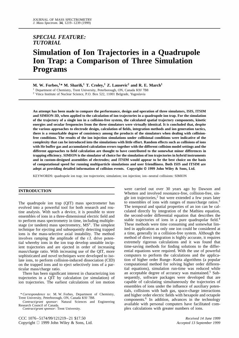
The common operating mode of an ion trap is withthe potential�0 applied to the ring electrode while theend-cap electrodes are grounded27 except when auxiliarypotentials are applied to either or both end-cap electrodes.The application of�0 to the ring electrode gives rise toa potential surface resembling a saddle and in Fig. 1 isillustrated an example of such a potential surface createdwith SIMION.
To perform computer simulations of ion motion in aQIT, the equations of the motion for trapped ions must beconsidered. The Mathieu equation was developed origi-nally to describe the regions of stability and instability onthe surface of a vibrating skin such as a drum.28 The clas-sical expression of the Mathieu equation is a second-orderdifferential identity:
d2u
d�2C .au � 2qu cos 2�/u D 0 .5/
Copyright 1999 John Wiley & Sons, Ltd. J. Mass Spectrom. 34, 1219–1239 (1999)
SIMULATION OF ION TRAJECTORIES IN A QUADRUPLE ION TRAP 1221
Figure 1. A potential surface generated by SIMION illustratingthe quadrupolar field inside the trap when the end-cap electrodesare grounded and a potential �0 is applied to the ring electrode.When t D 0, the potential rises from zero at the end-capelectrodes to �0/2 at the centre of the trap and rises againto �0 at the ring electrode.
where au and qu are dimensionlessstability parametersfor all of the coordinates (u) in the x, y and z directionsand � is equal to�t/2, where� is the radial frequencyof the r.f. drive potential applied to the ring electrode andt is time. By rearrangement of Eqn (5), substitution for� and multiplication of both sides of the equation by themass of the ion (m), Eqn (6) is obtained:
md2u
dt2D �m�
2
4.au � 2qu cos�t/u .6/
An ion of chargee in the field created by the applicationof a potential�0 on the ring electrode experiences a forceFx that is the product of ion mass and its acceleration inany directionx:
Fx D md2x
dt2D �e∂�x,y,z
∂xD �2ex
r02.U � VRF cos�t/ .7/
Similar expressions are obtained forFy andFz.From the solutions to the Mathieu equation that define
the conditions for realizing stable trajectories of ions inan ion trap, one obtains27
az D �2ar D � 16eU
mr02�2qz D �2qr D 8eV
mr02�2.8/
These relationships define the trapping parameters orworking point for each ion species according to thevoltages applied to the ion trap electrodes.
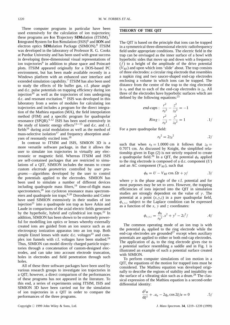
Commercial ion trap instruments operate in the primarystability region shown in Fig. 2. It is necessary to intro-duce two more trapping parameters (ˇr and ˇz) that, inconjunction withar , az and qr , qz, define the region ofsimultaneous stability in botha andq shown in Fig. 2. Thestability region is bounded by the iso-beta linesˇz D 0,ˇz D 1, ˇr D 0 andˇr D 1. When an ion has a stable tra-jectory, itsˇr andˇz values must be between 0 and 1 andan ion developing an unstable trajectory may be referredto as one whose working point (az, qz) has crossed one ofthese boundaries. Some of the intermediate iso-beta linesare indicated in Fig. 2. r and ˇz (herein referred to asˇu) is calculated by a complex progression ofau andqu.4
When the working point of an ion lies within thestability region, the ion is trapped successfully only when
Figure 2. The primary stability region plotted in az and qz withiso-beta lines included. The working points of ions in themass-selective axial instability mode lie on the qz axis, suchthat as the amplitude of the r.f. drive potential is ramped,the working points approach the ˇz D 1 boundary in order ofincreasing mass/charge ratio. The ˇz D 1 line intersects theqz-axis at qz D 0.908.
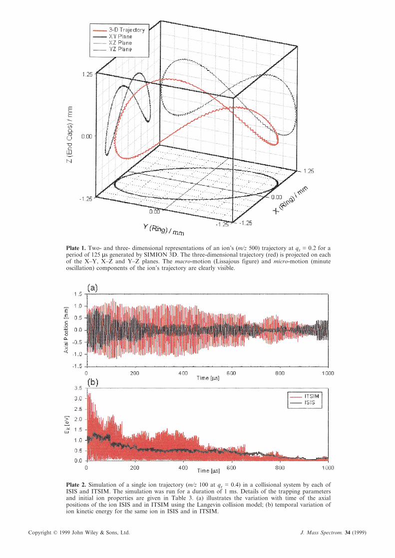
the boundsof its trajectory remain within the physicalconfinesof the ion trap. Under theseconditions,the ionwill assumea trajectorythatresemblesa figure-of-eightorLissajouscurve.Plate1 is a three-dimensionalplot of thetrajectoryof anion overa periodof 125 µs.TheLissajoustrajectoriesof trappedions(underr.f.-only conditions)aregenerallyconcentratedaboutthecentreof theion trap.Asthe working point of the ion is movedacrossthe stabilitydiagramtowardtheˇz D 1 boundary(qz D 0.908),theionattainsgreaterkinetic energies and the ion’s oscillationswithin the trap increasewith time. Theoscillatorymotionof anion is madeupof aprogressionof frequencies(ωu,n),wheren is an integer,and the frequenciesarecalculatedfrom the angularfrequencyandˇu asfollows:
ωu,n D š(nC 1
2ˇu)� .9/
The primary frequencies(for n D 0) of ωz and ωr areknown as the ion’s fundamentalsecularfrequencies.Itis this property of the ion’s motion that allows ions tobe ejectedselectively from the ion trap by applicationof a dipolar alternatingcurrent acrossthe end-capsinresonancewith the ion’s secularfrequency.The higher-orderfrequencies(n > 0) give rise to the micromotionofthe trajectoryin Plate1.
The ion trap in eachof the softwarepackagesconsid-eredis operatedwith voltagescalculatedfrom the theorypresentedhere. Each packagewas developedindepen-dently for the calculationof realistic ion trajectories.Inthis work, first, a detailed comparisonof some of theattributesof eachsimulation programis presented;sec-ond, the trajectory of a single ion under collision-freeconditionsis calculatedby eachprogram;andthird, sim-ulationsof ion injection havebeencarriedout underbothcollisional andcollison-freeconditions.
Copyright 1999JohnWiley & Sons,Ltd. J. MassSpectrom. 34, 1219–1239(1999)
1222 M. W. FORBESET AL.
THE SIMULATION PROGRAMS
Dialogue and operating system platform
The most notable differences between SIMION 6.0,ITSIM 4.1 and ISIS are their characteristics in userplatform. All three programs run on conventional PCsand all are computationally rigorous such that a powerfulcomplement of hardware is desirable for expedientrun times. All of the simulations with SIMION andITSIM were run on 366 MHz Pentium II processors with64 Mbytes of RAM and only one simulation was runat a given time. Each of the programs performs at adifferent rate and has widely different display functionsso, depending upon the application, the time required tocomplete a simulation was found to vary significantly.As expected, the dominating factor in determining runtime is the number of ions in the simulation. BothITSIM and SIMION allow simultaneous calculations ofthe trajectories of ensembles of ions while ISIS performssuccessive single-ion calculations.
ITSIM was first available in standard 640 kb DOS for-mat but the new version appears in a full Windows plat-form. ITSIM was written in CCC and makes of use ofWindows 32-bit memory-sharing capabilities.7 While theDOS versions of ITSIM utilized several input files for iondefinition, voltage programming, simulation run time, dataoutput, etc., ITSIM 4.1 combines all of these segmentsinto a user-friendly visual interface that allows simula-tions to be designed and run easily through single inputand executable files. ITSIM allows the user both to defineall of the conditions for an experiment prior to runningthe simulation and to change parameters during a simu-lation. Versatile time-dependent scan functions constitutean integral component of the software. ITSIM is a truemulti-particle simulator and can be used to characterizeboth single ion trajectories and those of large ensemblesof ions in a timely fashion.
ISIS, which was developed in the late 1980s and early1990s, runs in a DOS-based environment and utilizes adialogue similar to the early versions of ITSIM; the sim-ulation parameters are compiled from a series of inputfiles for scan functions, ion definition and data outputoptions. Since ISIS draws on a variety of modules duringthe course of the simulation, it requires a specific envi-ronment in which it is to be run and there is no optionto view ion trajectory data online or in real time. Rather,the experiments are formulated prior to running (as withITSIM) and the ion trajectory data are written to files forexamination after completion of the simulation. The var-ious modules of ISIS were written in either BASIC orFORTRAN6 and are compiled and run separately.
SIMION 6.0 differs from ITSIM and ISIS in bothdesign and user format. It offers an interactive dialoguein a DOS-based environment, but it is driven by a graph-ical user interface (GUI) of layered menus with mouse-activated buttons to guide the user from option to option.Unlike ITSIM and ISIS which are complete vehicles forsimulating ion trajectories in a QIT, SIMION requires thatthe user must develop his or her own electrode designs andmust write algorithms to perform such tasks as control-ling voltages and simulating collisions. On the other hand,SIMION has the versatility to model virtually any type
of mass spectrometer as well as ion optics and providesthe tools necessary to create and to run any such sim-ulation. The learning curve to proficiency with SIMIONcan be rather steep. The great versatility of SIMION isdemanding of a rigorous design procedure. The processesof creating electrodes, viewing structures, defining ions,running simulations and collecting data are all containedwithin SIMION’s menu system, and so it is comparable toITSIM. In contrast, the user programs comprise a separatecomponent and are typically written in a simple text, andso is comparable to ISIS. SIMION partitions the memoryavailable between that which is required for the size ofthe potential array and the number of ions that can beflown simultaneously. Thus, clouds of thousands of ionscan be simulated but, in practice, SIMION will run at anacceptable rate for only some 100–200 ions.
Electrode design
The design and calculation of the electric fields in thequadrupole ion trap form the root of the software’s abilityto calculate accurate charged particle trajectories whencoupled with a valid method of integration. SIMIONallows the user to create custom electrode geometrieswhereas ITSIM and ISIS are self-contained packages. ISISand ITSIM are capable of calculating ion trajectories inthe ideal, stretched and cylindrical ion trap geometries.Bui and Cooks7 have reported a novel six-electrode iontrap created with a modified version of ITSIM. It mustbe stressed that this comparative study only deals withITSIM version 4.1 since it was this version that wasmade available to the authors. A new version, ITSIM5.0, allows externally generated ions to fly into the iontrap volume through the holes in end-cap electrodes.In addition, ITSIM 5.0 permits the simulation of iontrajectories when ions are ejected through such holes andstrike a plane of detection.29–31
All of the simulations were carried out using the idealtrap geometry withr0 D 10 mm. The electrode surfaceswere created from continuous equations [as Eqn (1)], afeature innate to ISIS and ITSIM. However, the geometrydesign procedure is more rigorous for SIMION where thequality of the trajectory obtained is related directly to thequality of the electrode design created by the user.
The first component of SIMION’s electrode designinvolves producing a structure that approximates the shapeand dimensions of a real QIT. SIMION’s design capabil-ities allow the user to create a potential array (.PA) filewhich defines in space the bounds of the electrodes and theregions between the electrodes. Unlike ISIS and ITSIM,which build the electrodes in memory according to con-tinuous equations, the tools in SIMION’smodify dialogmust be employed to ensure accurate electrode geometry.Electrodes are created by filling in sections of pixels in thearray and voltages are assigned to the various electrodes.For complex designs in which the user wishes to con-trol dynamically the voltages on various electrodes, theelectrodes are numbered incrementally by their respectivevoltages. When the geometry is refined, a separate file iscreated for each electrode, e.g. *.pa1, *.pa2, etc. Tools areavailable to create various geometric shapes, so once thedimensions of the trap are known, it is possible to createaccurate hyperbolic electrodes as given by Eqn (1).
Copyright 1999 John Wiley & Sons, Ltd. J. Mass Spectrom. 34, 1219–1239 (1999)
Copyright © 1999 John Wiley & Sons, Ltd. J. Mass Spectrom. 34 (1999)
Plate 1. Two- and three- dimensional representations of an ion’s (m/z 500) trajectory at qz = 0.2 for aperiod of 125 µs generated by SIMION 3D. The three-dimensional trajectory (red) is projected on eachof the X–Y, X–Z and Y–Z planes. The macro-motion (Lissajous figure) and micro-motion (minuteoscillation) components of the ion’s trajectory are clearly visible.
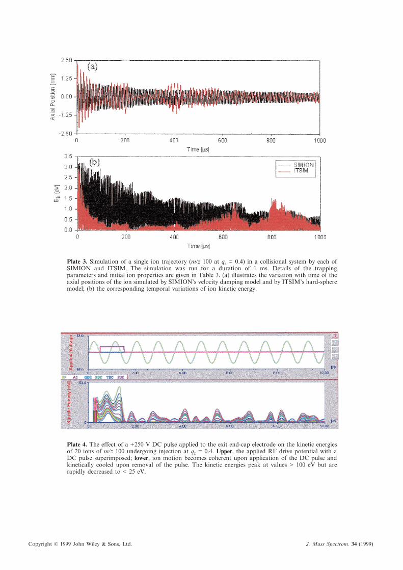
Plate 2. Simulation of a single ion trajectory (m/z 100 at qz = 0.4) in a collisional system by each ofISIS and ITSIM. The simulation was run for a duration of 1 ms. Details of the trapping parametersand initial ion properties are given in Table 3. (a) illustrates the variation with time of the axialpositions of the ion ISIS and in ITSIM using the Langevin collision model; (b) temporal variation ofion kinetic energy for the same ion in ISIS and in ITSIM.
Copyright © 1999 John Wiley & Sons, Ltd. J. Mass Spectrom. 34 (1999)
Plate 3. Simulation of a single ion trajectory (m/z 100 at qz = 0.4) in a collisional system by each ofSIMION and ITSIM. The simulation was run for a duration of 1 ms. Details of the trappingparameters and initial ion properties are given in Table 3. (a) illustrates the variation with time of theaxial positions of the ion simulated by SIMION’s velocity damping model and by ITSIM’s hard-spheremodel; (b) the corresponding temporal variations of ion kinetic energy.
Plate 4. The effect of a +250 V DC pulse applied to the exit end-cap electrode on the kinetic energiesof 20 ions of m/z 100 undergoing injection at qz = 0.4. Upper, the applied RF drive potential with aDC pulse superimposed; lower, ion motion becomes coherent upon application of the DC pulse andkinetically cooled upon removal of the pulse. The kinetic energies peak at values > 100 eV but arerapidly decreased to < 25 eV.
SIMULATION OF ION TRAJECTORIES IN A QUADRUPLE ION TRAP 1223
The second component of SIMION’s electrode designis the continuity of the surface; while rigorous hyperbolaecan be drawn, it is the resolution of the pixel arraythat determines ultimately the precision of the electrodesurface. To create a new electrode design the user mustspecify first the size of the density of the pixel arrayand then determine whether a two- or three-dimensionalstructure is to be built. Each pixel consumes 10 bytes ofconventional RAM such that for a three-dimensional cubicarray 100ð 100ð 100 pixels, 106 pixels will be usedand 10 Mbytes of RAM allotted in memory. When theelectrodes are created and the space between electrodes isrefined, any roughness in the electrode design translatesto a roughness in the calculated field, possibly introducinga significant source of error in the calculated trajectory.There are three factors that must be considered whenselecting the density of the pixel array: optimization oftrajectory quality, the limit of RAM in the PC and thespeed of the simulation run time.
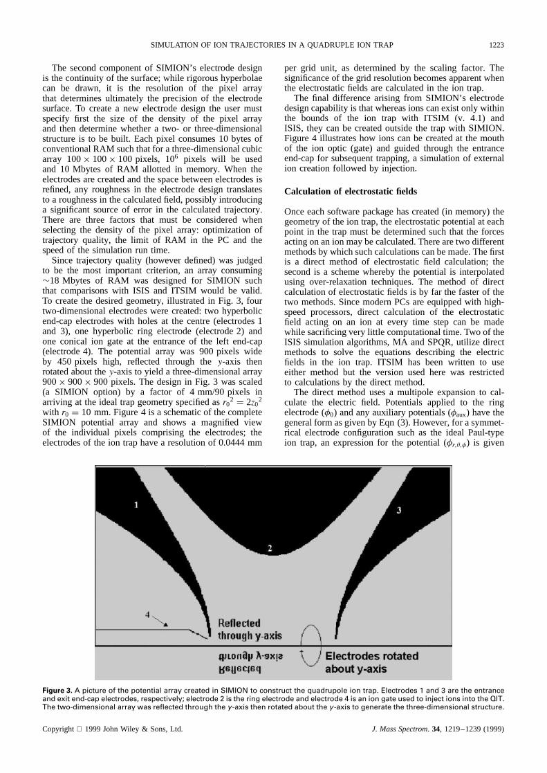
Since trajectory quality (however defined) was judgedto be the most important criterion, an array consuming¾18 Mbytes of RAM was designed for SIMION suchthat comparisons with ISIS and ITSIM would be valid.To create the desired geometry, illustrated in Fig. 3, fourtwo-dimensional electrodes were created: two hyperbolicend-cap electrodes with holes at the centre (electrodes 1and 3), one hyperbolic ring electrode (electrode 2) andone conical ion gate at the entrance of the left end-cap(electrode 4). The potential array was 900 pixels wideby 450 pixels high, reflected through they-axis thenrotated about they-axis to yield a three-dimensional array900ð 900ð 900 pixels. The design in Fig. 3 was scaled(a SIMION option) by a factor of 4 mm/90 pixels inarriving at the ideal trap geometry specified asr02 D 2z02
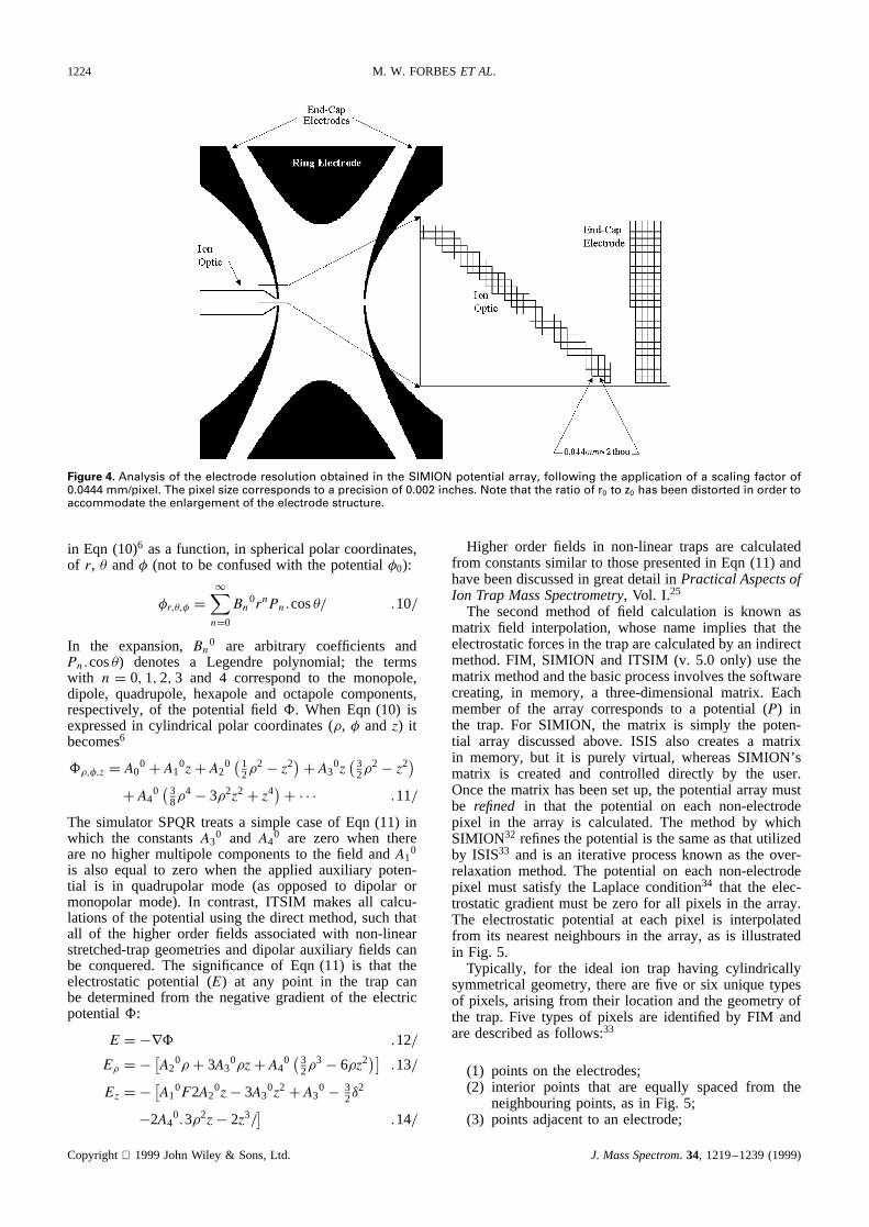
with r0 D 10 mm. Figure 4 is a schematic of the completeSIMION potential array and shows a magnified viewof the individual pixels comprising the electrodes; theelectrodes of the ion trap have a resolution of 0.0444 mm
per grid unit, as determined by the scaling factor. Thesignificance of the grid resolution becomes apparent whenthe electrostatic fields are calculated in the ion trap.
The final difference arising from SIMION’s electrodedesign capability is that whereas ions can exist only withinthe bounds of the ion trap with ITSIM (v. 4.1) andISIS, they can be created outside the trap with SIMION.Figure 4 illustrates how ions can be created at the mouthof the ion optic (gate) and guided through the entranceend-cap for subsequent trapping, a simulation of externalion creation followed by injection.
Calculation of electrostatic fields
Once each software package has created (in memory) thegeometry of the ion trap, the electrostatic potential at eachpoint in the trap must be determined such that the forcesacting on an ion may be calculated. There are two differentmethods by which such calculations can be made. The firstis a direct method of electrostatic field calculation; thesecond is a scheme whereby the potential is interpolatedusing over-relaxation techniques. The method of directcalculation of electrostatic fields is by far the faster of thetwo methods. Since modern PCs are equipped with high-speed processors, direct calculation of the electrostaticfield acting on an ion at every time step can be madewhile sacrificing very little computational time. Two of theISIS simulation algorithms, MA and SPQR, utilize directmethods to solve the equations describing the electricfields in the ion trap. ITSIM has been written to useeither method but the version used here was restrictedto calculations by the direct method.
The direct method uses a multipole expansion to cal-culate the electric field. Potentials applied to the ringelectrode (�0) and any auxiliary potentials (�aux) have thegeneral form as given by Eqn (3). However, for a symmet-rical electrode configuration such as the ideal Paul-typeion trap, an expression for the potential (�r,�,�) is given
Figure 3. A picture of the potential array created in SIMION to construct the quadrupole ion trap. Electrodes 1 and 3 are the entranceand exit end-cap electrodes, respectively; electrode 2 is the ring electrode and electrode 4 is an ion gate used to inject ions into the QIT.The two-dimensional array was reflected through the y-axis then rotated about the y-axis to generate the three-dimensional structure.
Copyright 1999 John Wiley & Sons, Ltd. J. Mass Spectrom. 34, 1219–1239 (1999)
1224 M. W. FORBESET AL.
Figure 4. Analysis of the electrode resolution obtained in the SIMION potential array, following the application of a scaling factor of0.0444 mm/pixel. The pixel size corresponds to a precision of 0.002 inches. Note that the ratio of r0 to z0 has been distorted in order toaccommodate the enlargement of the electrode structure.
in Eqn (10)6 asa function, in sphericalpolar coordinates,of r, � and� (not to be confusedwith the potential�0):
�r,�,� D1∑nD0
Bn0rnPn.cos�/ .10/
In the expansion,Bn0 are arbitrary coefficients andPn.cos�) denotes a Legendre polynomial; the termswith n D 0,1, 2, 3 and 4 correspondto the monopole,dipole, quadrupole,hexapoleand octapolecomponents,respectively,of the potential field . When Eqn (10) isexpressedin cylindrical polar coordinates(�, � and z) itbecomes6
�,�,z D A00 C A1
0z C A20 (1
2�2� z2)C A3
0z(3
2�2� z2)
C A40 ( 3
8�4� 3�2z2C z4)C Ð Ð Ð .11/
The simulatorSPQRtreatsa simple caseof Eqn (11) inwhich the constantsA3
0 and A40 are zero when there
are no higher multipole componentsto the field andA10
is also equal to zero when the applied auxiliary poten-tial is in quadrupolarmode (as opposedto dipolar ormonopolarmode). In contrast,ITSIM makesall calcu-lationsof the potentialusingthe direct method,suchthatall of the higher order fields associatedwith non-linearstretched-trapgeometriesanddipolar auxiliary fields canbe conquered.The significanceof Eqn (11) is that theelectrostaticpotential (E) at any point in the trap canbe determinedfrom the negativegradientof the electricpotential:
E D �r .12/
E� D �[A2
0� C 3A30�z C A4
0 (32�
3� 6�z2)]
.13/
Ez D �[A1
0F2A20z � 3A3
0z2C A30� 3
2υ2
�2A40.3�2z � 2z3/
].14/
Higher order fields in non-linear traps are calculatedfrom constantssimilar to thosepresentedin Eqn (11) andhavebeendiscussedin greatdetail in PracticalAspectsofIon Trap MassSpectrometry, Vol. I.25
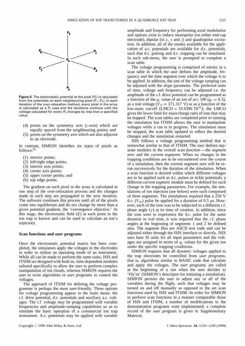
The secondmethod of field calculation is known asmatrix field interpolation,whosename implies that theelectrostaticforcesin thetraparecalculatedby anindirectmethod.FIM, SIMION and ITSIM (v. 5.0 only) usethematrix methodandthebasicprocessinvolvesthesoftwarecreating, in memory, a three-dimensionalmatrix. Eachmemberof the array correspondsto a potential (P) inthe trap. For SIMION, the matrix is simply the poten-tial array discussedabove. ISIS also createsa matrixin memory, but it is purely virtual, whereasSIMION’smatrix is createdand controlled directly by the user.Oncethe matrix hasbeensetup, the potentialarraymustbe refined in that the potential on each non-electrodepixel in the array is calculated.The method by whichSIMION32 refinesthepotentialis thesameasthatutilizedby ISIS33 and is an iterative processknown as the over-relaxationmethod.The potential on eachnon-electrodepixel must satisfy the Laplacecondition34 that the elec-trostaticgradientmustbe zerofor all pixels in the array.The electrostaticpotential at each pixel is interpolatedfrom its nearestneighboursin the array,as is illustratedin Fig. 5.
Typically, for the ideal ion trap having cylindricallysymmetricalgeometry,therearefive or six uniquetypesof pixels, arisingfrom their locationandthe geometryofthe trap. Five typesof pixels are identified by FIM andaredescribedasfollows:33
(1) pointson the electrodes;(2) interior points that are equally spacedfrom the
neighbouringpoints,as in Fig. 5;(3) pointsadjacentto an electrode;
Copyright 1999JohnWiley & Sons,Ltd. J. MassSpectrom. 34, 1219–1239(1999)
SIMULATION OF ION TRAJECTORIES IN A QUADRUPLE ION TRAP 1225
Figure 5. The electrostatic potential at the pixel (P0) is calculatedfrom the potentials on each neighbouring pixel (P1 P6). In eachiteration of the over-relaxation method, every pixel in the arrayis calculated as a P0 case and the iterations continue until thevoltage calculated for every P0 changes by less than a specifiedvalue.
(4) points on the symmetry axis (z-axis) which areequallyspacedfrom the neighbouringpoints;and
(5) pointson thesymmetryaxiswhicharealsoadjacentto an electrode.
In contrast, SIMION identifies six types of pixels asfollows:32
(1) interior points;(2) left/right edgepoints;(3) interior axis points;(4) corneraxis points;(5) uppercornerpoints;and(6) top edgepoints.
The gradienton eachpixel in the arrayis calculatedinone stepof the over-relaxationprocessand the changesmadein eachstep are propagatedto the next iteration.The softwarecontinuesthis processuntil all of the pixelscomeinto equilibrium anddo not changeby morethanagiven potentialgradient,the ‘convergenceobjective.’ Atthis stage,the electrostaticfield (E) at eachpoint in theion trap is known and can be usedto calculatean ion’strajectory.
Scanfunctions and user programs
Once the electrostaticpotential matrix has been com-pleted,the simulatorsapply the voltagesto the electrodesin order to realize an operatingmode of an instrument.While all canbemadeto performthesametasks,ISISandITSIM aredesignedwith built-in, time-dependentmodulestailoredspecificallyto allow the userto performcomplexmanipulationof ion clouds,whereasSIMION requirestheuserto write algorithmsor userprograms to control thevoltages.
The approachof ITSIM for defining the voltage pro-grammeis perhapsthe most user-friendly.Threeoptionsfor voltage programmingappearin the main menu: ther.f. drive potential,d.c. potentialsandauxiliary a.c.volt-ages.The r.f. voltagemay be programmedwith variablefrequenciesand amplitude-rampingcapabilitiesso as tosimulate the basic operationof a commercial ion trapinstrument.A.c. potentialsmay be appliedwith variable
amplitudeandfrequencyfor performingaxial modulationandoptionsexist to inducemonopolar(on eitherend-capelectrode),dipolar (in x, y andz) andquadrupolarexcita-tion. In addition,all of the modesavailablefor the appli-cation of a.c. potentialsare availablefor d.c. potentials,suchthat d.c. pulsingandd.c. trappingcanbe simulated.In eachsub-menu,the user is promptedto completeascantable.
The voltageprogrammingis comprisedof entriesin ascantable in which the user definesthe amplitude,fre-quencyandthe time segmentoverwhich thevoltageis tobeapplied.In addition,therateof thevoltagerampingcanbe adjustedwith the slopeparameter.The preferredunitsof time, voltage and frequencycan be adjustedi.e. theamplitudeof ther.f. drive potentialcanbeprogrammedasa functionof theqz valueof an ion of m/z 100(qz D 0.3),asa realvoltage(Vrf D 371.317 V) or asa functionof thelow-masscut-off (LMCO D 33.0396Th35); the LMCOgivesthelower limit for mass/chargeratioof ionsthatmaybetrapped.Thescantablesarecompletedprior to runningthe simulationbut ITSIM allows the user to manipulatevoltageswhile a run is in progress.The simulationmustbe stopped,the scantable updatedto reflect the desiredchangesandthe simulationrestarted.
ISIS follows a voltage programmingmethod that issomewhatsimilar to thatof ITSIM. The userdefinessep-aratemodulesin the overall scanfunction—the segmentzero and the current segments. When no changesin thetrappingconditionsareto be encounteredover the courseof a simulation,thenthe currentsegmentzerowill be re-run successivelyfor the durationof the simulation.Whena scanfunction is desiredwithin which differentvoltagesareto beappliedsuchasd.c.pulsesor tickle potentials,adifferentcurrentsegmentmodulemustbedefinedfor eachchangein the trappingparameters.For example,the sim-ulationsof ion injection (seebelow)wereeachcomprisedof threesegments.The simulationsrequiredthat a 250 Vd.c. (Vdc) pulsebe appliedfor a durationof 0.5 µs. How-ever,eachof theionswasto besubjectedto adifferentr.f.phaseangle( ) at its time of creation.In addition,sincethe ions were to experiencethe d.c. pulse for the sameduration in real time, it was requiredthat the r.f. phaseanglesat the beginningof segments1 and 2 be definedalso. The segmentfiles are ASCII text codeand can beadjustedeitherthroughthe ISIS interfaceor directly. ISISusesbaseSI units for all input parametersand the volt-agesareassignedin termsof qz valuesfor the given ionunderthe specifictrappingconditions.
SIMION requiresthat all dynamicvoltagesappliedtothe trap electrodesbe controlled from user programs,that is, algorithmssimilar to BASIC code that calculateand apply the voltages.The user programs are calledat the beginning of a run when the user decides to‘Fly’m’ (SIMION’s descriptorfor initiating a simulation).SIMION permits the user to adjust any or all of thevariablesduring the flight, such that voltages may beturned on and off manually as opposedto the set scanfunctionsusedby ISIS andITSIM. In orderfor SIMIONto performscanfunctionsin a mannercomparablethoseof ISIS and ITSIM, a number of modifications to thedemonstrationprogramswere implemented;a completerecord of the user program is given in SupplementaryMaterial.
Copyright 1999JohnWiley & Sons,Ltd. J. MassSpectrom. 34, 1219–1239(1999)
1226 M. W. FORBESET AL.
Whereas ITSIM allows the user to select the units oftime, voltage and frequency by which the scan tablesare created and ISIS user SI units, SIMION accepts andreturns values (in the user program) in units of atomicmass units, volts, eV, mm andµs; thus, any conversionsfrom values input according to more familiar conventionsmust be incorporated in the user program.
Ion definition
An ion’s identity is defined by the parameters mass(m), charge (e), initial position (x,y,z), initial velocity inrectangular Cartesian coordinates (Px, Py, Pz) or polar three-dimensional coordinates (kinetic energy (Ek), azimuth (�),elevation (�)), time of creation (t) and cross-sectionalarea (�). Of these parameters, SIMION and ISIS con-sider all but�. Since ITSIM can simulate ion–neutralcollisions with a hard-sphere collision model, it requiresthat � be defined for each ion. SIMION utilizes polarthree-dimensional coordinates to specify the ion’s ini-tial velocity and uses kinetic energy with units of eV tospecify the magnitude. ITSIM and ISIS accept initial ionproperties inx, y andz coordinates.
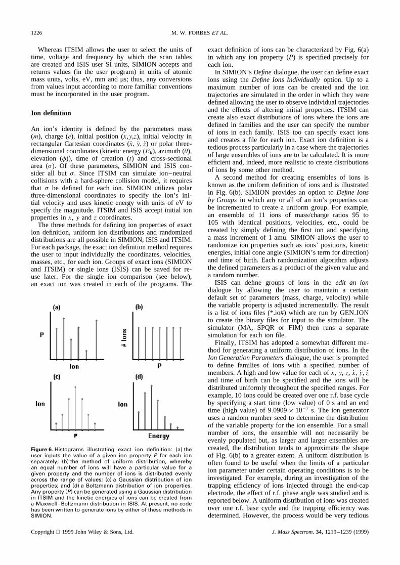
The three methods for defining ion properties of exaction definition, uniform ion distributions and randomizeddistributions are all possible in SIMION, ISIS and ITSIM.For each package, the exact ion definition method requiresthe user to input individually the coordinates, velocities,masses, etc., for each ion. Groups of exact ions (SIMIONand ITSIM) or single ions (ISIS) can be saved for re-use later. For the single ion comparison (see below),an exact ion was created in each of the programs. The
Figure 6. Histograms illustrating exact ion definition: (a) theuser inputs the value of a given ion property P for each ionseparately; (b) the method of uniform distribution, wherebyan equal number of ions will have a particular value for agiven property and the number of ions is distributed evenlyacross the range of values; (c) a Gaussian distribution of ionproperties; and (d) a Boltzmann distribution of ion properties.Any property (P) can be generated using a Gaussian distributionin ITSIM and the kinetic energies of ions can be created froma Maxwell Boltzmann distribution in ISIS. At present, no codehas been written to generate ions by either of these methods inSIMION.
exactdefinition of ions canbe characterizedby Fig. 6(a)in which any ion property (P) is specifiedpreciselyforeachion.
In SIMION’s Definedialogue,theusercandefineexactions using the DefineIons Individually option. Up to amaximum number of ions can be createdand the iontrajectoriesaresimulatedin the orderin which they weredefinedallowing theuserto observeindividual trajectoriesand the effects of altering initial properties.ITSIM cancreatealso exactdistributionsof ions wherethe ions aredefinedin families and the usercan specify the numberof ions in eachfamily. ISIS too can specify exact ionsand createsa file for eachion. Exact ion definition is atediousprocessparticularlyin acasewherethetrajectoriesof largeensemblesof ions areto becalculated.It is moreefficient and,indeed,morerealisticto createdistributionsof ions by someothermethod.
A secondmethod for creating ensemblesof ions isknown asthe uniform definition of ions andis illustratedin Fig. 6(b). SIMION providesan option to DefineIonsby Groups in which any or all of an ion’s propertiescanbe incrementedto createa uniform group.For example,an ensembleof 11 ions of mass/charge ratios 95 to105 with identical positions, velocities, etc., could becreatedby simply defining the first ion and specifyinga massincrementof 1 amu.SIMION allows the user torandomizeion propertiessuchas ions’ positions,kineticenergies,initial coneangle(SIMION’s termfor direction)and time of birth. Eachrandomizationalgorithm adjuststhedefinedparametersasa productof thegivenvalueanda randomnumber.
ISIS can define groups of ions in the edit an iondialogue by allowing the user to maintain a certaindefault set of parameters(mass,charge, velocity) whilethevariablepropertyis adjustedincrementally.Theresultis a list of ions files (*.io#) which are run by GEN IONto createthe binary files for input to the simulator.Thesimulator (MA, SPQR or FIM) then runs a separatesimulationfor eachion file.
Finally, ITSIM hasadopteda somewhatdifferent me-thod for generatinga uniform distribution of ions. In theIon GenerationParametersdialogue,theuseris promptedto define families of ions with a specifiednumber ofmembers.A high andlow valuefor eachof x, y, z, Px, Py, Pzand time of birth can be specifiedand the ions will bedistributeduniformly throughoutthespecifiedranges.Forexample,10 ionscouldbecreatedoveroner.f. basecycleby specifyinga start time (low value) of 0 s and an endtime (high value) of 9.0909ð 10�7 s. The ion generatorusesa randomnumberseedto determinethe distributionof the variablepropertyfor the ion ensemble.For a smallnumber of ions, the ensemblewill not necessarilybeevenly populatedbut, as larger and larger ensemblesarecreated,the distribution tendsto approximatethe shapeof Fig. 6(b) to a greaterextent.A uniform distribution isoften found to be useful when the limits of a particularion parameterundercertainoperatingconditionsis to beinvestigated.For example,during an investigationof thetrapping efficiency of ions injected through the end-capelectrode,the effect of r.f. phaseanglewasstudiedandisreportedbelow.A uniformdistributionof ionswascreatedover one r.f. basecycle and the trappingefficiency wasdetermined.However,the processwould be very tedious
Copyright 1999JohnWiley & Sons,Ltd. J. MassSpectrom. 34, 1219–1239(1999)
SIMULATION OF ION TRAJECTORIES IN A QUADRUPLE ION TRAP 1227
if each ion were to be created manually by exact iondefinition.
The third method of ion creation generates ions withproperties varied according to a Gaussian distributionas illustrated in Fig. 6(c) or a Maxwell–Boltzmann-likedistribution as shown in Fig. 6(d). ISIS has a functionincluded by which the initial kinetic energies of an ensem-ble of ions can be generated from a Boltzmann distributionof energies. Real populations of ions under set conditionswill have energies that can be described by the familiarfunction36
ni D Ne�{ εikT
}∑j
gj e�{εjkT
} .15/
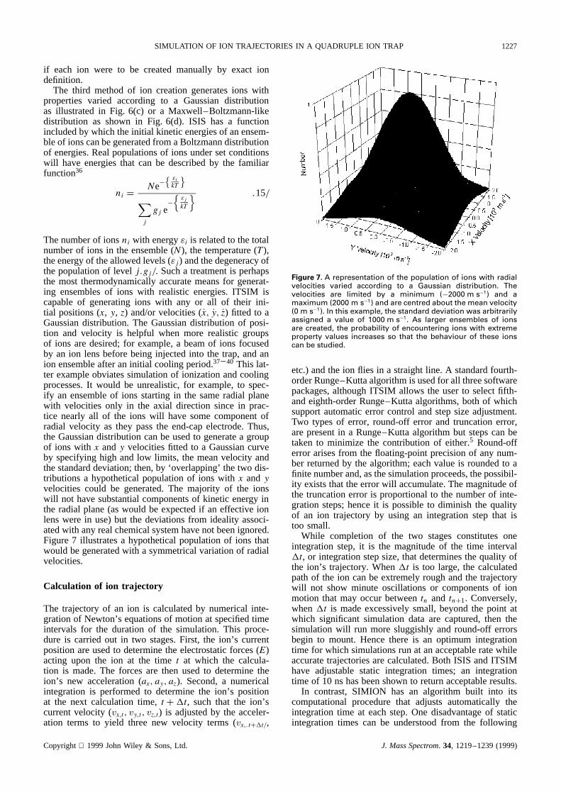
The number of ionsni with energyεi is related to the totalnumber of ions in the ensemble (N), the temperature (T),the energy of the allowed levels (εj) and the degeneracy ofthe population of levelj.gj/. Such a treatment is perhapsthe most thermodynamically accurate means for generat-ing ensembles of ions with realistic energies. ITSIM iscapable of generating ions with any or all of their ini-tial positions (x, y, z) and/or velocities (Px, Py, Pz) fitted to aGaussian distribution. The Gaussian distribution of posi-tion and velocity is helpful when more realistic groupsof ions are desired; for example, a beam of ions focusedby an ion lens before being injected into the trap, and anion ensemble after an initial cooling period.37–40 This lat-ter example obviates simulation of ionization and coolingprocesses. It would be unrealistic, for example, to spec-ify an ensemble of ions starting in the same radial planewith velocities only in the axial direction since in prac-tice nearly all of the ions will have some component ofradial velocity as they pass the end-cap electrode. Thus,the Gaussian distribution can be used to generate a groupof ions with x andy velocities fitted to a Gaussian curveby specifying high and low limits, the mean velocity andthe standard deviation; then, by ‘overlapping’ the two dis-tributions a hypothetical population of ions withx andyvelocities could be generated. The majority of the ionswill not have substantial components of kinetic energy inthe radial plane (as would be expected if an effective ionlens were in use) but the deviations from ideality associ-ated with any real chemical system have not been ignored.Figure 7 illustrates a hypothetical population of ions thatwould be generated with a symmetrical variation of radialvelocities.
Calculation of ion trajectory
The trajectory of an ion is calculated by numerical inte-gration of Newton’s equations of motion at specified timeintervals for the duration of the simulation. This proce-dure is carried out in two stages. First, the ion’s currentposition are used to determine the electrostatic forces (E)acting upon the ion at the timet at which the calcula-tion is made. The forces are then used to determine theion’s new acceleration (ax, ay, az). Second, a numericalintegration is performed to determine the ion’s positionat the next calculation time,t Ct, such that the ion’scurrent velocity (vx,t, vy,t, vz,t) is adjusted by the acceler-ation terms to yield three new velocity terms (vx,.tCt/,
Figure 7. A representation of the population of ions with radialvelocities varied according to a Gaussian distribution. Thevelocities are limited by a minimum (�2000 m s�1) and amaximum (2000 m s�1) and are centred about the mean velocity(0 m s�1). In this example, the standard deviation was arbitrarilyassigned a value of 1000 m s�1. As larger ensembles of ionsare created, the probability of encountering ions with extremeproperty values increases so that the behaviour of these ionscan be studied.
etc.)andthe ion flies in a straightline. A standardfourth-orderRunge–Kuttaalgorithmis usedfor all threesoftwarepackages,althoughITSIM allows the userto selectfifth-andeighth-orderRunge–Kutta algorithms,both of whichsupportautomaticerror control andstepsizeadjustment.Two typesof error, round-off error and truncationerror,arepresentin a Runge–Kutta algorithmbut stepscanbetakento minimize the contributionof either.5 Round-offerrorarisesfrom the floating-pointprecisionof any num-ber returnedby the algorithm;eachvalueis roundedto afinite numberand,asthesimulationproceeds,thepossibil-ity existsthat theerrorwill accumulate.Themagnitudeofthe truncationerror is proportionalto the numberof inte-grationsteps;henceit is possibleto diminish the qualityof an ion trajectory by using an integrationstep that istoo small.
While completion of the two stagesconstitutesoneintegrationstep, it is the magnitudeof the time intervalt, or integrationstepsize,thatdeterminesthequality ofthe ion’s trajectory.Whent is too large, the calculatedpathof the ion canbe extremelyroughandthe trajectorywill not show minute oscillationsor componentsof ionmotion that may occurbetweentn and tnC1. Conversely,whent is madeexcessivelysmall, beyondthe point atwhich significant simulation data are captured,then thesimulationwill run moresluggishlyand round-off errorsbegin to mount. Hencethere is an optimum integrationtime for which simulationsrun at anacceptableratewhileaccuratetrajectoriesarecalculated.Both ISIS andITSIMhave adjustablestatic integration times; an integrationtime of 10 nshasbeenshownto returnacceptableresults.
In contrast,SIMION has an algorithm built into itscomputationalprocedurethat adjusts automatically theintegrationtime at eachstep.One disadvantageof staticintegrationtimes can be understoodfrom the following
Copyright 1999JohnWiley & Sons,Ltd. J. MassSpectrom. 34, 1219–1239(1999)
1228 M. W. FORBESET AL.
analogy. When one is driving on a rough road withsteep hills, the driver controls vehicle speed based onreaction time to unforeseen obstacles. In this way, whena large drop-off is reached, the vehicle’s momentum willbe sufficiently low that the vehicle is not propelled overthe edge and remains on the road. In the same way, anion trajectory simulator can blindly propel an ion over alarge potential barrier and miss an important componentof an ion’s motion. In order to obviate this problem,SIMION calculates one integration step ahead and if theion’s kinetic energy is found to change dramatically, theintegration step-size is halved. The integration time isreduced successively until changes in the ion’s kineticenergy reach a maximum limit. SIMION also permitsthe integration time to increase so as to minimize run-time. A maximum limit of 10 ns was applied in the userprogram to ensure a trajectory quality comparable to ISISand ITSIM.
Since integration time plays an important role in thequality of a calculated trajectory, the 10 ns time used byISIS and ITSIM was used as a benchmark for SIMION.SIMION permits control of a factor called thetrajectoryquality, which can take values from�500 to C500;a setting of zero turns off SIMION’s velocity reversaldetection, edge detection and binary boundary approach.32
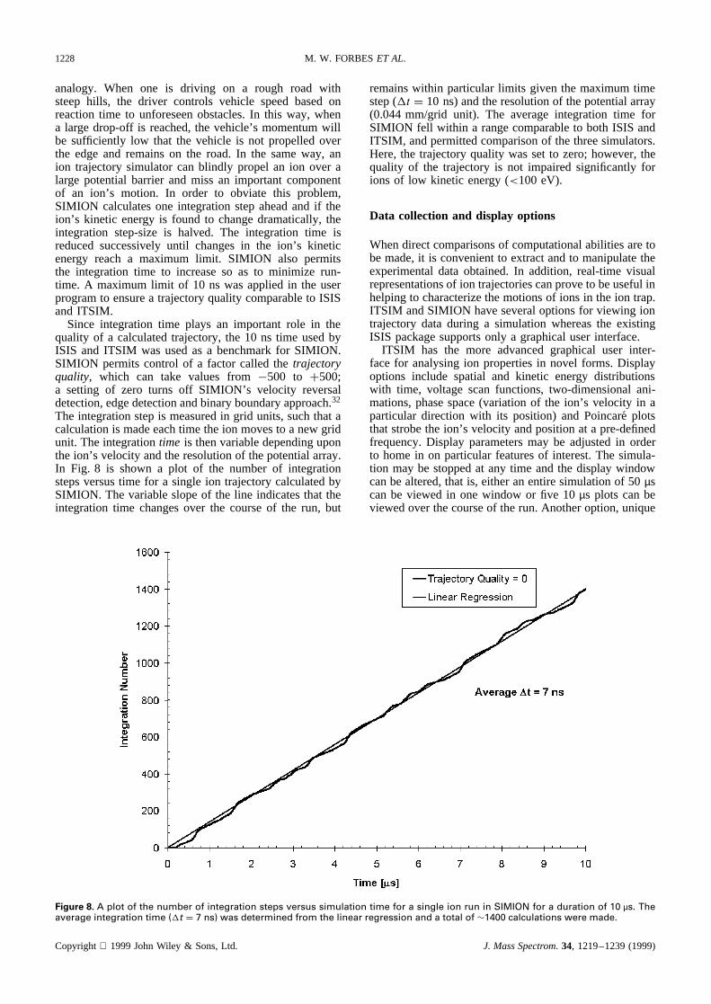
The integration step is measured in grid units, such that acalculation is made each time the ion moves to a new gridunit. The integrationtime is then variable depending uponthe ion’s velocity and the resolution of the potential array.In Fig. 8 is shown a plot of the number of integrationsteps versus time for a single ion trajectory calculated bySIMION. The variable slope of the line indicates that theintegration time changes over the course of the run, but
remains within particular limits given the maximum timestep (t D 10 ns) and the resolution of the potential array(0.044 mm/grid unit). The average integration time forSIMION fell within a range comparable to both ISIS andITSIM, and permitted comparison of the three simulators.Here, the trajectory quality was set to zero; however, thequality of the trajectory is not impaired significantly forions of low kinetic energy (<100 eV).
Data collection and display options
When direct comparisons of computational abilities are tobe made, it is convenient to extract and to manipulate theexperimental data obtained. In addition, real-time visualrepresentations of ion trajectories can prove to be useful inhelping to characterize the motions of ions in the ion trap.ITSIM and SIMION have several options for viewing iontrajectory data during a simulation whereas the existingISIS package supports only a graphical user interface.
ITSIM has the more advanced graphical user inter-face for analysing ion properties in novel forms. Displayoptions include spatial and kinetic energy distributionswith time, voltage scan functions, two-dimensional ani-mations, phase space (variation of the ion’s velocity in aparticular direction with its position) and Poincare plotsthat strobe the ion’s velocity and position at a pre-definedfrequency. Display parameters may be adjusted in orderto home in on particular features of interest. The simula-tion may be stopped at any time and the display windowcan be altered, that is, either an entire simulation of 50µscan be viewed in one window or five 10µs plots can beviewed over the course of the run. Another option, unique
Figure 8. A plot of the number of integration steps versus simulation time for a single ion run in SIMION for a duration of 10 µs. Theaverage integration time (t D 7 ns) was determined from the linear regression and a total of ¾1400 calculations were made.
Copyright 1999JohnWiley & Sons,Ltd. J. MassSpectrom. 34, 1219–1239(1999)
SIMULATION OF ION TRAJECTORIES IN A QUADRUPLE ION TRAP 1229
to ITSIM, is the ability to generate mass spectra fromdetected ions. At the end of a simulation, parameters suchas mass/charge ratio, time of detection, r.f. phase angleat ejection, position, velocity and collision counts can beplotted in the form of a mass spectrum. Since much flex-ibility has been built into the detection options, the useris offered a powerful method for the rapid examination ofsimulation data in a concise presentation.
SIMION’s display functions are designed to accommo-date the analysis of ion trajectories in three-dimensionalstructures of any electrode geometry. Thus, although iondata can be captured, real-time display options are gearedtowards complex two- and three-dimensional visualiza-tions. The electrodes may be viewed in any orientationand at virtually any magnification. It was found that theversatility of the graphical representation of the ion trapand ion trajectories was extremely helpful in developinga feel for the behaviour of ions under various conditions.An example is the three-dimensional representation ofion injection (see below) whereby ions are sprayed bythe ion gate through the end-cap electrode; it was pos-sible, using SIMION, to view the ions up-close as theyentered the ion trap. In addition to the normal 2D and 3Dmodes, SIMION provides a third viewing option, that ofthe potential energy view (PE View), an example of whichappears in Fig. 1.
The second means for analyzing simulation data is tocapture various properties of the ion (e.g. time, position,velocity, etc.) at specified intervals. All of the softwarepackages are capable of capturing simulation data for eachion at every integration step or at larger time intervals. Thedata are written to a file in comma or tab delimited ASCIIformat, such that they can be imported into spreadsheetor scientific graphing software packages. SIMION allowsthe capture of numerical data for each ion flown in amultiparticle simulation, whereas ITSIM will write thedata for one ion at a time. Thus, single-ion trajectoriesmust be run if the user wishes to export data for an ionensemble.
A major concern when analysing extracted data is thatthe files can become extremely large for a short exper-imental time. For example, a typical QIT will perform
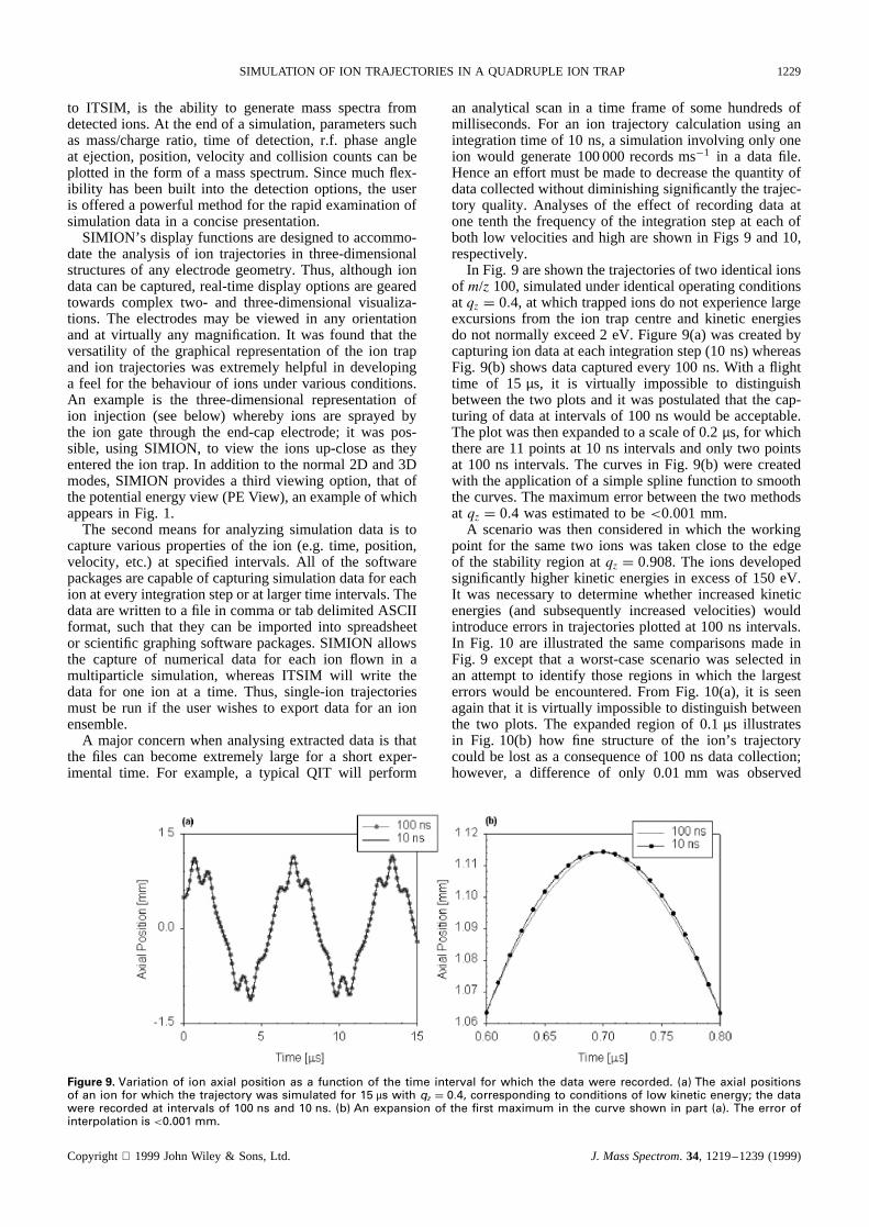
an analytical scan in a time frame of some hundreds ofmilliseconds. For an ion trajectory calculation using anintegration time of 10 ns, a simulation involving only oneion would generate 100 000 records ms�1 in a data file.Hence an effort must be made to decrease the quantity ofdata collected without diminishing significantly the trajec-tory quality. Analyses of the effect of recording data atone tenth the frequency of the integration step at each ofboth low velocities and high are shown in Figs 9 and 10,respectively.
In Fig. 9 are shown the trajectories of two identical ionsof m/z 100, simulated under identical operating conditionsat qz D 0.4, at which trapped ions do not experience largeexcursions from the ion trap centre and kinetic energiesdo not normally exceed 2 eV. Figure 9(a) was created bycapturing ion data at each integration step (10 ns) whereasFig. 9(b) shows data captured every 100 ns. With a flighttime of 15µs, it is virtually impossible to distinguishbetween the two plots and it was postulated that the cap-turing of data at intervals of 100 ns would be acceptable.The plot was then expanded to a scale of 0.2µs, for whichthere are 11 points at 10 ns intervals and only two pointsat 100 ns intervals. The curves in Fig. 9(b) were createdwith the application of a simple spline function to smooththe curves. The maximum error between the two methodsat qz D 0.4 was estimated to be<0.001 mm.
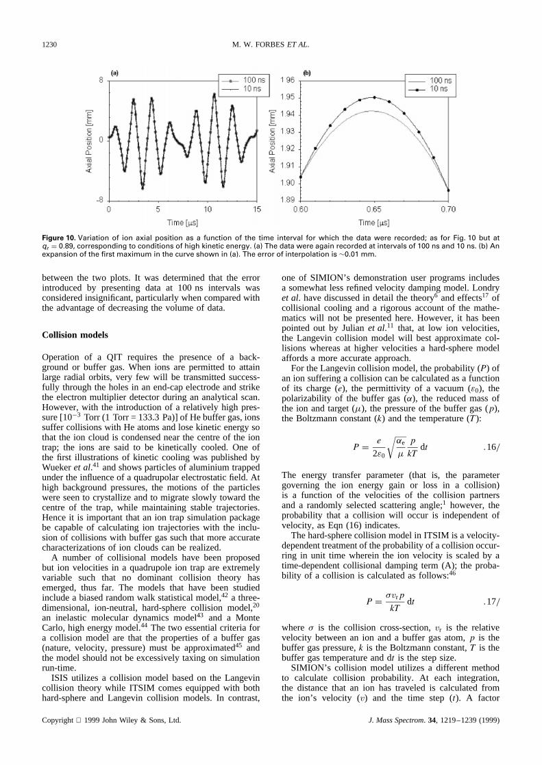
A scenario was then considered in which the workingpoint for the same two ions was taken close to the edgeof the stability region atqz D 0.908. The ions developedsignificantly higher kinetic energies in excess of 150 eV.It was necessary to determine whether increased kineticenergies (and subsequently increased velocities) wouldintroduce errors in trajectories plotted at 100 ns intervals.In Fig. 10 are illustrated the same comparisons made inFig. 9 except that a worst-case scenario was selected inan attempt to identify those regions in which the largesterrors would be encountered. From Fig. 10(a), it is seenagain that it is virtually impossible to distinguish betweenthe two plots. The expanded region of 0.1µs illustratesin Fig. 10(b) how fine structure of the ion’s trajectorycould be lost as a consequence of 100 ns data collection;however, a difference of only 0.01 mm was observed
Figure 9. Variation of ion axial position as a function of the time interval for which the data were recorded. (a) The axial positionsof an ion for which the trajectory was simulated for 15 µs with qz D 0.4, corresponding to conditions of low kinetic energy; the datawere recorded at intervals of 100 ns and 10 ns. (b) An expansion of the first maximum in the curve shown in part (a). The error ofinterpolation is <0.001 mm.
Copyright 1999JohnWiley & Sons,Ltd. J. MassSpectrom. 34, 1219–1239(1999)
1230 M. W. FORBESET AL.
Figure 10. Variation of ion axial position as a function of the time interval for which the data were recorded; as for Fig. 10 but atqz D 0.89, corresponding to conditions of high kinetic energy. (a) The data were again recorded at intervals of 100 ns and 10 ns. (b) Anexpansion of the first maximum in the curve shown in (a). The error of interpolation is ¾0.01 mm.
betweenthe two plots. It was determinedthat the errorintroduced by presentingdata at 100 ns intervals wasconsideredinsignificant,particularlywhencomparedwiththe advantageof decreasingthe volumeof data.
Collision models
Operation of a QIT requires the presenceof a back-groundor buffer gas.When ions are permittedto attainlarge radial orbits, very few will be transmittedsuccess-fully throughthe holesin an end-capelectrodeandstrikethe electronmultiplier detectorduring an analyticalscan.However,with the introductionof a relatively high pres-sure[10�3 Torr (1 Torr = 133.3Pa)]of Hebuffer gas,ionssuffer collisionswith He atomsandlosekinetic energy sothat the ion cloud is condensednearthe centreof the iontrap; the ions are said to be kinetically cooled. One ofthe first illustrationsof kinetic cooling waspublishedbyWuekeret al.41 andshowsparticlesof aluminiumtrappedunderthe influenceof a quadrupolarelectrostaticfield. Athigh backgroundpressures,the motions of the particleswereseento crystallizeandto migrateslowly towardthecentreof the trap, while maintainingstabletrajectories.Henceit is importantthat an ion trap simulationpackagebe capableof calculatingion trajectorieswith the inclu-sion of collisionswith buffer gassuchthat moreaccuratecharacterizationsof ion cloudscanbe realized.
A number of collisional models have beenproposedbut ion velocitiesin a quadrupoleion trap areextremelyvariable such that no dominant collision theory hasemerged, thus far. The models that have been studiedincludea biasedrandomwalk statisticalmodel,42 a three-dimensional,ion-neutral,hard-spherecollision model,20
an inelastic molecular dynamicsmodel43 and a MonteCarlo,high energy model.44 The two essentialcriteria fora collision model are that the propertiesof a buffer gas(nature,velocity, pressure)must be approximated45 andthe modelshouldnot be excessivelytaxing on simulationrun-time.
ISIS utilizes a collision model basedon the Langevincollision theory while ITSIM comesequippedwith bothhard-sphereand Langevin collision models.In contrast,
one of SIMION’s demonstrationuserprogramsincludesa somewhatlessrefinedvelocity dampingmodel.Londryet al. havediscussedin detail the theory6 andeffects17 ofcollisional cooling and a rigorousaccountof the mathe-maticswill not be presentedhere.However,it hasbeenpointedout by Julian et al.11 that, at low ion velocities,the Langevincollision model will bestapproximatecol-lisions whereasat higher velocitiesa hard-spheremodelaffords a moreaccurateapproach.
For theLangevincollision model,theprobability(P) ofanion suffering a collision canbecalculatedasa functionof its charge (e), the permittivity of a vacuum(ε0), thepolarizability of the buffer gas(˛), the reducedmassofthe ion andtarget (�), the pressureof the buffer gas(p),the Boltzmannconstant(k) andthe temperature(T):
P D e
2ε0
√˛e
�
p
kTdt .16/
The energy transfer parameter(that is, the parametergoverning the ion energy gain or loss in a collision)is a function of the velocities of the collision partnersand a randomlyselectedscatteringangle;1 however,theprobability that a collision will occur is independentofvelocity, asEqn (16) indicates.
Thehard-spherecollision modelin ITSIM is a velocity-dependenttreatmentof theprobabilityof acollisionoccur-ring in unit time whereinthe ion velocity is scaledby atime-dependentcollisional dampingterm (A); the proba-bility of a collision is calculatedasfollows:46
P D �vrp
kTdt .17/
where� is the collision cross-section,vr is the relativevelocity betweenan ion and a buffer gasatom,p is thebuffer gaspressure,k is the Boltzmannconstant,T is thebuffer gastemperatureanddt is the stepsize.
SIMION’s collision model utilizes a different methodto calculate collision probability. At each integration,the distancethat an ion has traveledis calculatedfromthe ion’s velocity (v) and the time step (t). A factor
Copyright 1999JohnWiley & Sons,Ltd. J. MassSpectrom. 34, 1219–1239(1999)
SIMULATION OF ION TRAJECTORIES IN A QUADRUPLE ION TRAP 1231
called ‘mean-free-path’ (MFP) is then used to calculatea collision factor (CF) as in Eqn (18):
CF D 1� e�vt
MFP .18/
The calculated velocity-dependentCF is compared with arandom number between zero and one; when the randomnumber is>CF, a collision occurs and the ion’s velocityis adjusted in accordance with Eqn (19) to obtain the newvelocity,Vnew:
VnewD v(mion � mbuffer
mion C mbuffer
).19/
wheremion andmbuffer are the masses of the ion and buffergas, respectively.
RESULTS
Single ion comparison in a collision-free system
The basic comparison of the three simulators involvedcalculation of the trajectories of three identical ions havingidentical trapping parameters in a collision-free system.From these simulations, a detailed comparison of theions’ spatial (radial and axial) variations with time, kineticenergy.Ek/ variations with time and secular frequencieswas made. In Table 1 is presented a summary of thetrapping parameters and initial ion properties for thesimulations and in Table 2 are presented some numericalresults. The simulations were run for 25µs and the datawere collected at an output increment of 10 ns. Sincethe duration of the simulation was short and since anexact comparison was to be made, simulation data wereaccumulated at 10 ns intervals to eliminate uncertainty inthe comparison.
For ISIS, initially, a software package called UnGraph(Biosoft) was used to obtain numerical data from graph-ical output. The ‘UnGraphing’ process scales a scannedimage and traces the plot to generate a series of data.While UnGraph yielded acceptable results for visual pre-sentations of the ion trajectory data, minor errors wereintroduced due to resolution limitations of the image.
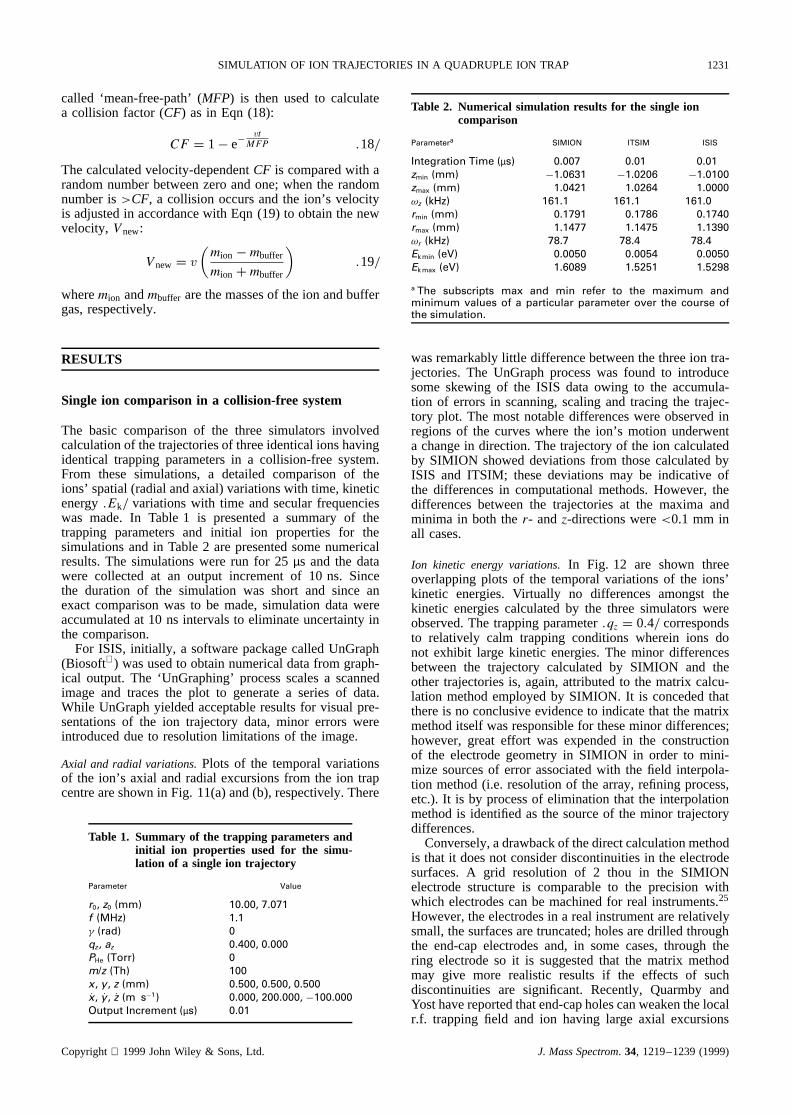
Axial and radial variations.Plots of the temporal variationsof the ion’s axial and radial excursions from the ion trapcentre are shown in Fig. 11(a) and (b), respectively. There
Table 1. Summary of the trapping parameters andinitial ion properties used for the simu-lation of a single ion trajectory
Parameter Value
r0, z0 (mm) 10.00, 7.071f (MHz) 1.1 (rad) 0qz, az 0.400, 0.000PHe (Torr) 0m/z (Th) 100x, y, z (mm) 0.500, 0.500, 0.500Px, Py, Pz (m s�1) 0.000, 200.000, �100.000Output Increment (µs) 0.01
Table 2. Numerical simulation results for the single ioncomparison
Parametera SIMION ITSIM ISIS
Integration Time (µs) 0.007 0.01 0.01zmin (mm) �1.0631 �1.0206 �1.0100zmax (mm) 1.0421 1.0264 1.0000ωz (kHz) 161.1 161.1 161.0rmin (mm) 0.1791 0.1786 0.1740rmax (mm) 1.1477 1.1475 1.1390ωr (kHz) 78.7 78.4 78.4Ek min (eV) 0.0050 0.0054 0.0050Ek max (eV) 1.6089 1.5251 1.5298
a The subscripts max and min refer to the maximum andminimum values of a particular parameter over the course ofthe simulation.
was remarkably little difference between the three ion tra-jectories. The UnGraph process was found to introducesome skewing of the ISIS data owing to the accumula-tion of errors in scanning, scaling and tracing the trajec-tory plot. The most notable differences were observed inregions of the curves where the ion’s motion underwenta change in direction. The trajectory of the ion calculatedby SIMION showed deviations from those calculated byISIS and ITSIM; these deviations may be indicative ofthe differences in computational methods. However, thedifferences between the trajectories at the maxima andminima in both ther- andz-directions were<0.1 mm inall cases.
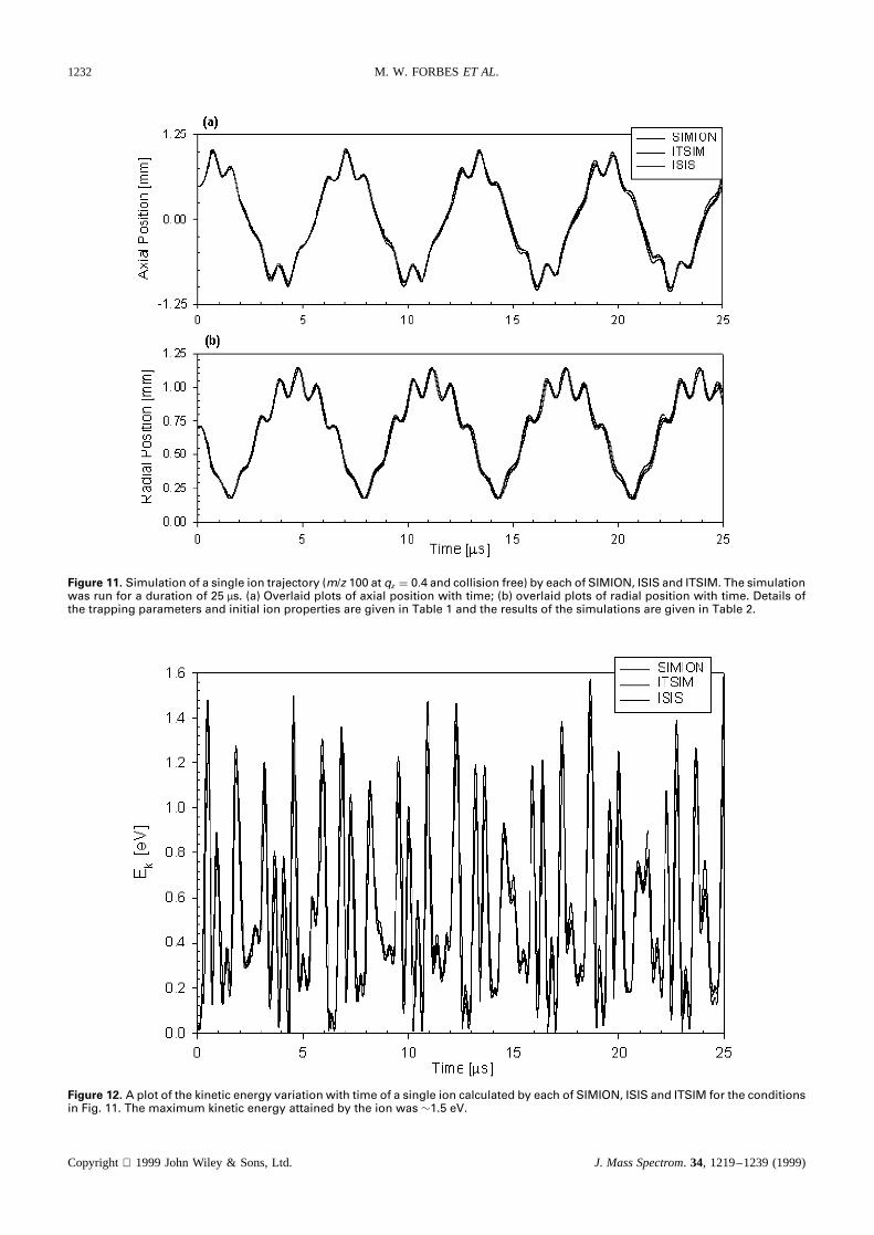
Ion kinetic energy variations.In Fig. 12 are shown threeoverlapping plots of the temporal variations of the ions’kinetic energies. Virtually no differences amongst thekinetic energies calculated by the three simulators wereobserved. The trapping parameter.qz D 0.4/ correspondsto relatively calm trapping conditions wherein ions donot exhibit large kinetic energies. The minor differencesbetween the trajectory calculated by SIMION and theother trajectories is, again, attributed to the matrix calcu-lation method employed by SIMION. It is conceded thatthere is no conclusive evidence to indicate that the matrixmethod itself was responsible for these minor differences;however, great effort was expended in the constructionof the electrode geometry in SIMION in order to mini-mize sources of error associated with the field interpola-tion method (i.e. resolution of the array, refining process,etc.). It is by process of elimination that the interpolationmethod is identified as the source of the minor trajectorydifferences.
Conversely, a drawback of the direct calculation methodis that it does not consider discontinuities in the electrodesurfaces. A grid resolution of 2 thou in the SIMIONelectrode structure is comparable to the precision withwhich electrodes can be machined for real instruments.25
However, the electrodes in a real instrument are relativelysmall, the surfaces are truncated; holes are drilled throughthe end-cap electrodes and, in some cases, through thering electrode so it is suggested that the matrix methodmay give more realistic results if the effects of suchdiscontinuities are significant. Recently, Quarmby andYost have reported that end-cap holes can weaken the localr.f. trapping field and ion having large axial excursions
Copyright 1999 John Wiley & Sons, Ltd. J. Mass Spectrom. 34, 1219–1239 (1999)
1232 M. W. FORBESET AL.
Figure 11. Simulation of a single ion trajectory (m/z 100 at qz D 0.4 and collision free) by each of SIMION, ISIS and ITSIM. The simulationwas run for a duration of 25 µs. (a) Overlaid plots of axial position with time; (b) overlaid plots of radial position with time. Details ofthe trapping parameters and initial ion properties are given in Table 1 and the results of the simulations are given in Table 2.
Figure 12. A plot of the kinetic energy variation with time of a single ion calculated by each of SIMION, ISIS and ITSIM for the conditionsin Fig. 11. The maximum kinetic energy attained by the ion was ¾1.5 eV.
Copyright 1999JohnWiley & Sons,Ltd. J. MassSpectrom. 34, 1219–1239(1999)
SIMULATION OF ION TRAJECTORIES IN A QUADRUPLE ION TRAP 1233
(as they do in ion injection) are more susceptible tothis distortion of the field.47 Although the trajectoriesof SIMION appear to stand apart from those of ISISand ITSIM, it should not be concluded that SIMIONcalculations are any more or less accurate than those ofISIS and ITSIM.
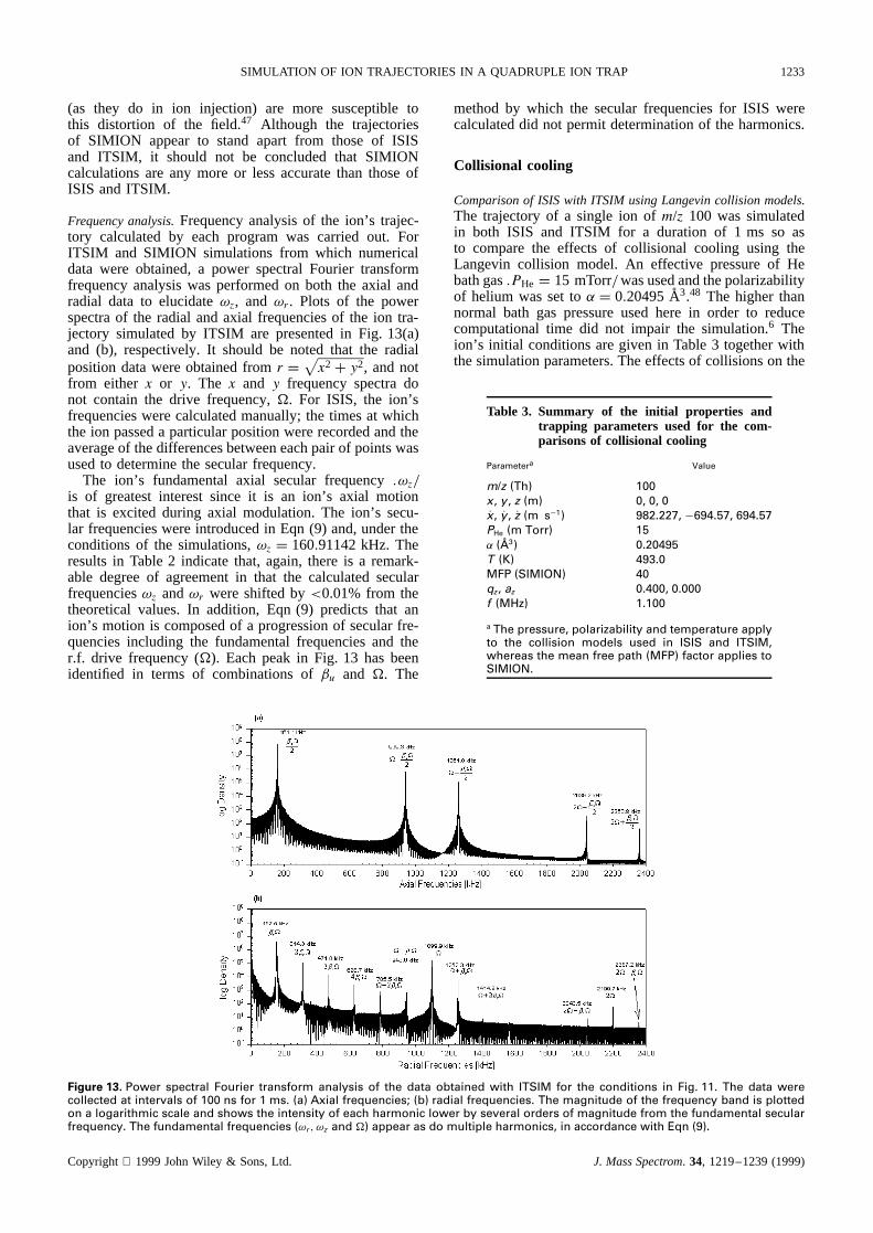
Frequency analysis.Frequency analysis of the ion’s trajec-tory calculated by each program was carried out. ForITSIM and SIMION simulations from which numericaldata were obtained, a power spectral Fourier transformfrequency analysis was performed on both the axial andradial data to elucidateωz, and ωr . Plots of the powerspectra of the radial and axial frequencies of the ion tra-jectory simulated by ITSIM are presented in Fig. 13(a)and (b), respectively. It should be noted that the radialposition data were obtained fromr D√x2C y2, and notfrom either x or y. The x and y frequency spectra donot contain the drive frequency,�. For ISIS, the ion’sfrequencies were calculated manually; the times at whichthe ion passed a particular position were recorded and theaverage of the differences between each pair of points wasused to determine the secular frequency.
The ion’s fundamental axial secular frequency.ωz/is of greatest interest since it is an ion’s axial motionthat is excited during axial modulation. The ion’s secu-lar frequencies were introduced in Eqn (9) and, under theconditions of the simulations,ωz D 160.91142 kHz. Theresults in Table 2 indicate that, again, there is a remark-able degree of agreement in that the calculated secularfrequenciesωz andωr were shifted by<0.01% from thetheoretical values. In addition, Eqn (9) predicts that anion’s motion is composed of a progression of secular fre-quencies including the fundamental frequencies and ther.f. drive frequency (�). Each peak in Fig. 13 has beenidentified in terms of combinations ofu and �. The
method by which the secular frequencies for ISIS werecalculated did not permit determination of the harmonics.
Collisional cooling
Comparison of ISIS with ITSIM using Langevin collision models.The trajectory of a single ion ofm/z 100 was simulatedin both ISIS and ITSIM for a duration of 1 ms so asto compare the effects of collisional cooling using theLangevin collision model. An effective pressure of Hebath gas.PHe D 15 mTorr/ was used and the polarizabilityof helium was set to D 0.20495A3.48 The higher thannormal bath gas pressure used here in order to reducecomputational time did not impair the simulation.6 Theion’s initial conditions are given in Table 3 together withthe simulation parameters. The effects of collisions on the
Table 3. Summary of the initial properties andtrapping parameters used for the com-parisons of collisional cooling
Parametera Value
m/z (Th) 100x, y, z (m) 0, 0, 0Px, Py, Pz (m s�1) 982.227, �694.57, 694.57PHe (m Torr) 15˛ (A3) 0.20495T (K) 493.0MFP (SIMION) 40qz, az 0.400, 0.000f (MHz) 1.100
a The pressure, polarizability and temperature applyto the collision models used in ISIS and ITSIM,whereas the mean free path (MFP) factor applies toSIMION.
Figure 13. Power spectral Fourier transform analysis of the data obtained with ITSIM for the conditions in Fig. 11. The data werecollected at intervals of 100 ns for 1 ms. (a) Axial frequencies; (b) radial frequencies. The magnitude of the frequency band is plottedon a logarithmic scale and shows the intensity of each harmonic lower by several orders of magnitude from the fundamental secularfrequency. The fundamental frequencies (ωr , ωz and �) appear as do multiple harmonics, in accordance with Eqn (9).
Copyright 1999JohnWiley & Sons,Ltd. J. MassSpectrom. 34, 1219–1239(1999)
1234 M. W. FORBESET AL.
ion’s axial position and kinetic energy as a result of usingthe Langevin collision model are shown in Plate 2(a) and(b), respectively. The results generated by ISIS and byITSIM showed that the trends in condensation of ionmotion and reduction of kinetic energy to be in goodagreement. The similarity of the models is illustrated bythe observation that the ion simulated by ISIS suffered149 collisions while the ion simulated by ITSIM suffered151 collisions. It was concluded that both the probabilitycalculations and the collision energy factors were verysimilar. Note that the ISIS data were collected at 1000 nsintervals as compared with 100 ns intervals from ITSIMsince the operating system configurations restricted thevolume of data collected in a run. However, the ISISresults give an accurate representation of kinetic coolingfor comparison with ITSIM.
Comparison of velocity-damping (SIMION) and hard-sphere(ITSIM) collision models.A comparison, similar to thatabove, was made between the velocity-damping modelof SIMION and the hard-sphere model of ITSIM;the simulation parameters are reported in Table 3. InPlate 3(a) and (b) are shown plots of the temporalvariations in ion axial position and ion kinetic energyversus time, respectively. In each of Plate 3(a) and (b) areplotted the data obtained with SIMION and with ITSIM.The mean free path setting in SIMION (MFPD 40) wasfound to approximate the effects of a pressure of Hebuffer gas of 15 mTorr in ITSIM using a collisional cross-section,�, equal to 50A2. Some experiments were runto test lower values of the SIMION MFP factor so asto approximate better the decrease in ion kinetic energythat occurs in the first 100µs of the ITSIM simulation.However, when lower values of the MFP are used inSIMION, Eqn (18) indicates that the probability of acollision increases exponentially, i.e. the velocity willbe damped much more rapidly. In addition, SIMION’scollision model does not allow for positive energycollisions. Although the hard-sphere model induces a morerapid decline in kinetic energy over the first 100µs ofthe simulation in ITSIM, lower values of the MFP werefound to decrease excessively the ion’s kinetic energy overlonger simulation periods.
Ion injection
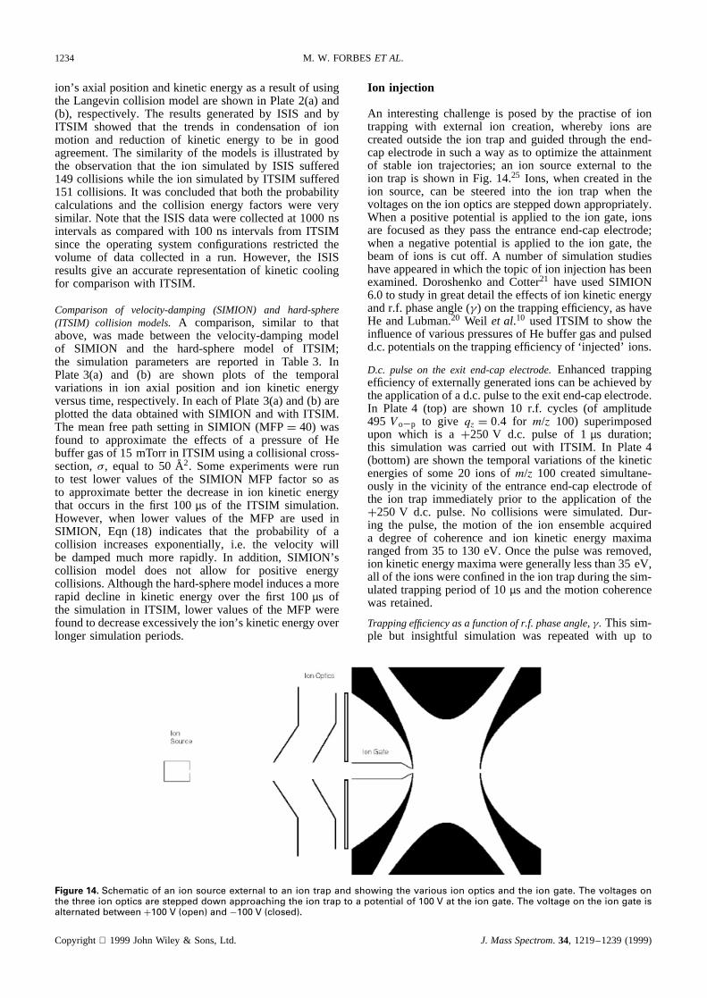
An interesting challenge is posed by the practise of iontrapping with external ion creation, whereby ions arecreated outside the ion trap and guided through the end-cap electrode in such a way as to optimize the attainmentof stable ion trajectories; an ion source external to theion trap is shown in Fig. 14.25 Ions, when created in theion source, can be steered into the ion trap when thevoltages on the ion optics are stepped down appropriately.When a positive potential is applied to the ion gate, ionsare focused as they pass the entrance end-cap electrode;when a negative potential is applied to the ion gate, thebeam of ions is cut off. A number of simulation studieshave appeared in which the topic of ion injection has beenexamined. Doroshenko and Cotter21 have used SIMION6.0 to study in great detail the effects of ion kinetic energyand r.f. phase angle ( ) on the trapping efficiency, as haveHe and Lubman.20 Weil et al.10 used ITSIM to show theinfluence of various pressures of He buffer gas and pulsedd.c. potentials on the trapping efficiency of ‘injected’ ions.
D.c. pulse on the exit end-cap electrode.Enhanced trappingefficiency of externally generated ions can be achieved bythe application of a d.c. pulse to the exit end-cap electrode.In Plate 4 (top) are shown 10 r.f. cycles (of amplitude495Vo–p to give qz D 0.4 for m/z 100) superimposedupon which is aC250 V d.c. pulse of 1µs duration;this simulation was carried out with ITSIM. In Plate 4(bottom) are shown the temporal variations of the kineticenergies of some 20 ions ofm/z 100 created simultane-ously in the vicinity of the entrance end-cap electrode ofthe ion trap immediately prior to the application of theC250 V d.c. pulse. No collisions were simulated. Dur-ing the pulse, the motion of the ion ensemble acquireda degree of coherence and ion kinetic energy maximaranged from 35 to 130 eV. Once the pulse was removed,ion kinetic energy maxima were generally less than 35 eV,all of the ions were confined in the ion trap during the sim-ulated trapping period of 10µs and the motion coherencewas retained.
Trapping efficiency as a function of r.f. phase angle, . This sim-ple but insightful simulation was repeated with up to
Figure 14. Schematic of an ion source external to an ion trap and showing the various ion optics and the ion gate. The voltages onthe three ion optics are stepped down approaching the ion trap to a potential of 100 V at the ion gate. The voltage on the ion gate isalternated between C100 V (open) and �100 V (closed).
Copyright 1999JohnWiley & Sons,Ltd. J. MassSpectrom. 34, 1219–1239(1999)
SIMULATION OF ION TRAJECTORIES IN A QUADRUPLE ION TRAP 1235
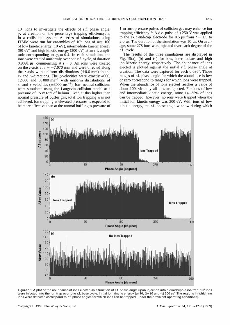
105 ions to investigate the effects of r.f. phase angle, , at creation on the percentage trapping efficiency,ε,in a collisional system. A series of simulations usingITSIM were run for ensembles of 105 ions of m/z 100of low kinetic energy (10 eV), intermediate kinetic energy(80 eV) and high kinetic energy (300 eV) at an r.f. ampli-tude corresponding toqz D 0.4. In each simulation, theions were created uniformly over one r.f. cycle, of duration0.9091µs, commencing att D 0. All ions were createdon thez-axis atz D �7.070 mm and were directed alongthe z-axis with uniform distributions (š0.6 mm) in thex- and y-directions. Thez-velocities were exactly 4000,12 000 and 30 000 ms�1 with uniform distributions ofx- andy-velocities (š3000 ms�1). Ion–neutral collisionswere simulated using the Langevin collision model at apressure of 15 mTorr of helium. Even at this higher thannormal pressure of buffer gas, total ion trapping was notachieved. Ion trapping at elevated pressures is expected tobe more effective than at the normal buffer gas pressure of
1 mTorr, pressure pulses of collision gas may enhance iontrapping efficiency.49 A d.c. pulse ofC250 V was appliedto the exit end-cap electrode for 0.5µs from t D 1.5 to2.0 µs. The duration of the simulation was 10µs. On aver-age, some 278 ions were injected over each degree of ther.f. cycle.
The results of the three simulations are displayed inFig. 15(a), (b) and (c) for low, intermediate and highion kinetic energy, respectively. The abundance of ionsejected is plotted against the initial r.f. phase angle atcreation. The data were captured for each 0.036°. Thoseranges of r.f. phase angle for which the abundance is lowor zero correspond to ranges for which ions were trapped.When the abundance of ions ejected reaches a value ofabout 100, virtually all ions are ejected. For ions of lowand intermediate kinetic energy, some 14–35% of ionscan be trapped; however, no ions were trapped when theinitial ion kinetic energy was 300 eV. With ions of lowkinetic energy, the r.f. phase angle window during which
Figure 15. A plot of the abundance of ions ejected as a function of r.f. phase angle upon injection into a quadrupole ion trap. 105 ionswere injected into the ion trap over one r.f. base cycle. Initial ion kinetic energy (a) 10, (b) 80 and (c) 300 eV. The regions in which noions were detected correspond to r.f. phase angles for which ions can be trapped (under the prevalent operating conditions).
Copyright 1999 John Wiley & Sons, Ltd. J. Mass Spectrom. 34, 1219–1239 (1999)
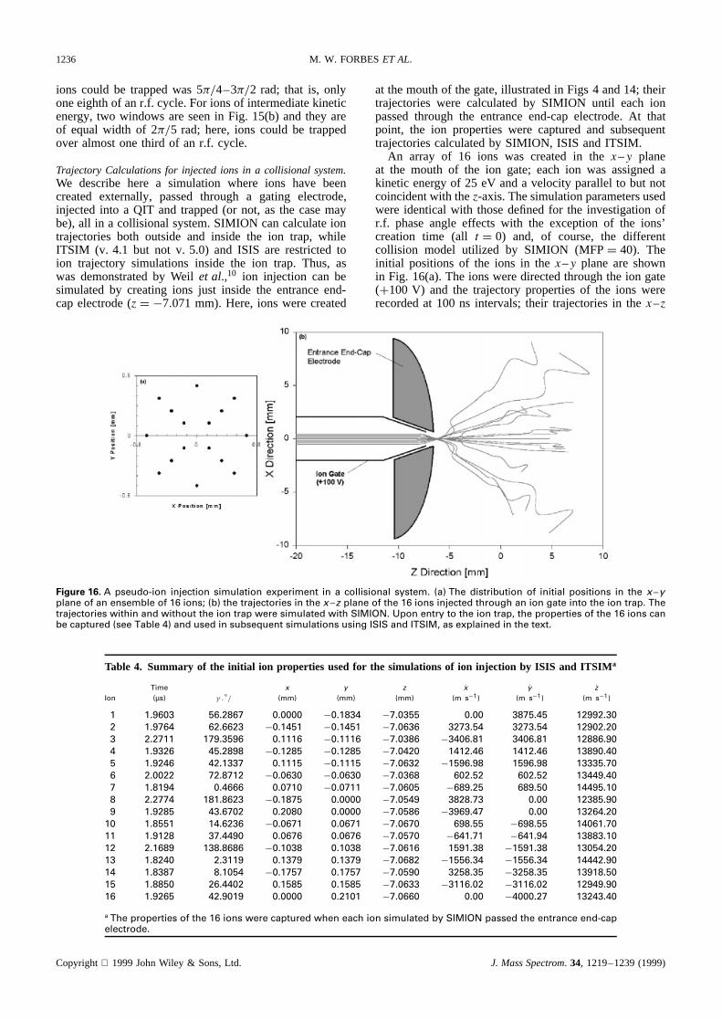
1236 M. W. FORBESET AL.
ions could be trapped was 5�/4–3�/2 rad; that is, onlyone eighth of an r.f. cycle. For ions of intermediate kineticenergy, two windows are seen in Fig. 15(b) and they areof equal width of 2�/5 rad; here, ions could be trappedover almost one third of an r.f. cycle.
Trajectory Calculations for injected ions in a collisional system.We describe here a simulation where ions have beencreated externally, passed through a gating electrode,injected into a QIT and trapped (or not, as the case maybe), all in a collisional system. SIMION can calculate iontrajectories both outside and inside the ion trap, whileITSIM (v. 4.1 but not v. 5.0) and ISIS are restricted toion trajectory simulations inside the ion trap. Thus, aswas demonstrated by Weilet al.,10 ion injection can besimulated by creating ions just inside the entrance end-cap electrode (z D �7.071 mm). Here, ions were created
at the mouth of the gate, illustrated in Figs 4 and 14; theirtrajectories were calculated by SIMION until each ionpassed through the entrance end-cap electrode. At thatpoint, the ion properties were captured and subsequenttrajectories calculated by SIMION, ISIS and ITSIM.
An array of 16 ions was created in thex–y planeat the mouth of the ion gate; each ion was assigned akinetic energy of 25 eV and a velocity parallel to but notcoincident with thez-axis. The simulation parameters usedwere identical with those defined for the investigation ofr.f. phase angle effects with the exception of the ions’creation time (all t D 0) and, of course, the differentcollision model utilized by SIMION (MFPD 40). Theinitial positions of the ions in thex–y plane are shownin Fig. 16(a). The ions were directed through the ion gate(C100 V) and the trajectory properties of the ions wererecorded at 100 ns intervals; their trajectories in thex–z
Figure 16. A pseudo-ion injection simulation experiment in a collisional system. (a) The distribution of initial positions in the x yplane of an ensemble of 16 ions; (b) the trajectories in the x z plane of the 16 ions injected through an ion gate into the ion trap. Thetrajectories within and without the ion trap were simulated with SIMION. Upon entry to the ion trap, the properties of the 16 ions canbe captured (see Table 4) and used in subsequent simulations using ISIS and ITSIM, as explained in the text.
Table 4. Summary of the initial ion properties used for the simulations of ion injection by ISIS and ITSIMa
Time x y z Px Py PzIon (µs) .°/ (mm) (mm) (mm) (m s�1) (m s�1) (m s�1)
1 1.9603 56.2867 0.0000 �0.1834 �7.0355 0.00 3875.45 12992.302 1.9764 62.6623 �0.1451 �0.1451 �7.0636 3273.54 3273.54 12902.203 2.2711 179.3596 0.1116 �0.1116 �7.0386 �3406.81 3406.81 12886.904 1.9326 45.2898 �0.1285 �0.1285 �7.0420 1412.46 1412.46 13890.405 1.9246 42.1337 0.1115 �0.1115 �7.0632 �1596.98 1596.98 13335.706 2.0022 72.8712 �0.0630 �0.0630 �7.0368 602.52 602.52 13449.407 1.8194 0.4666 0.0710 �0.0711 �7.0605 �689.25 689.50 14495.108 2.2774 181.8623 �0.1875 0.0000 �7.0549 3828.73 0.00 12385.909 1.9285 43.6702 0.2080 0.0000 �7.0586 �3969.47 0.00 13264.20
10 1.8551 14.6236 �0.0671 0.0671 �7.0670 698.55 �698.55 14061.7011 1.9128 37.4490 0.0676 0.0676 �7.0570 �641.71 �641.94 13883.1012 2.1689 138.8686 �0.1038 0.1038 �7.0616 1591.38 �1591.38 13054.2013 1.8240 2.3119 0.1379 0.1379 �7.0682 �1556.34 �1556.34 14442.9014 1.8387 8.1054 �0.1757 0.1757 �7.0590 3258.35 �3258.35 13918.5015 1.8850 26.4402 0.1585 0.1585 �7.0633 �3116.02 �3116.02 12949.9016 1.9265 42.9019 0.0000 0.2101 �7.0660 0.00 �4000.27 13243.40
a The properties of the 16 ions were captured when each ion simulated by SIMION passed the entrance end-capelectrode.
Copyright 1999 John Wiley & Sons, Ltd. J. Mass Spectrom. 34, 1219–1239 (1999)
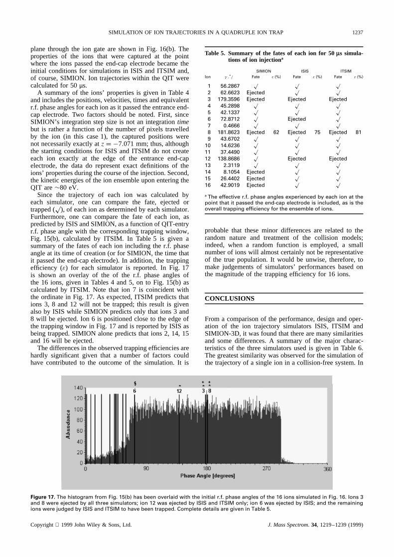
SIMULATION OF ION TRAJECTORIES IN A QUADRUPLE ION TRAP 1237
plane through the ion gate are shown in Fig. 16(b). Theproperties of the ions that were captured at the pointwhere the ions passed the end-cap electrode became theinitial conditions for simulations in ISIS and ITSIM and,of course, SIMION. Ion trajectories within the QIT werecalculated for 50µs.
A summary of the ions’ properties is given in Table 4and includes the positions, velocities, times and equivalentr.f. phase angles for each ion as it passed the entrance end-cap electrode. Two factors should be noted. First, sinceSIMION’s integration step size is not an integrationtimebut is rather a function of the number of pixels travelledby the ion (in this case 1), the captured positions werenot necessarily exactly atz D �7.071 mm; thus, althoughthe starting conditions for ISIS and ITSIM do not createeach ion exactly at the edge of the entrance end-capelectrode, the data do represent exact definitions of theions’ properties during the course of the injection. Second,the kinetic energies of the ion ensemble upon entering theQIT are¾80 eV.
Since the trajectory of each ion was calculated byeach simulator, one can compare the fate, ejected ortrapped (
p), of each ion as determined by each simulator.
Furthermore, one can compare the fate of each ion, aspredicted by ISIS and SIMION, as a function of QIT-entryr.f. phase angle with the corresponding trapping window,Fig. 15(b), calculated by ITSIM. In Table 5 is given asummary of the fates of each ion including the r.f. phaseangle at its time of creation (or for SIMION, the time thatit passed the end-cap electrode). In addition, the trappingefficiency (ε) for each simulator is reported. In Fig. 17is shown an overlay of the of the r.f. phase angles ofthe 16 ions, given in Tables 4 and 5, on to Fig. 15(b) ascalculated by ITSIM. Note that ion 7 is coincident withthe ordinate in Fig. 17. As expected, ITSIM predicts thations 3, 8 and 12 will not be trapped; this result is givenalso by ISIS while SIMION predicts only that ions 3 and8 will be ejected. Ion 6 is positioned close to the edge ofthe trapping window in Fig. 17 and is reported by ISIS asbeing trapped. SIMION alone predicts that ions 2, 14, 15and 16 will be ejected.
The differences in the observed trapping efficiencies arehardly significant given that a number of factors couldhave contributed to the outcome of the simulation. It is
Table 5. Summary of the fates of each ion for 50µs simula-tions of ion injectiona
SIMION ISIS ITSIMIon .°/ Fate ε (%) Fate ε (%) Fate ε (%)
1 56.2867p p p
2 62.6623 Ejectedp p
3 179.3596 Ejected Ejected Ejected4 45.2898
p p p5 42.1337
p p p6 72.8712
pEjected
p7 0.4666
p p p8 181.8623 Ejected 62 Ejected 75 Ejected 819 43.6702
p p p10 14.6236
p p p11 37.4490
p p p12 138.8686
pEjected Ejected
13 2.3119p p p
14 8.1054 Ejectedp p
15 26.4402 Ejectedp p
16 42.9019 Ejectedp p
a The effective r.f. phase angles experienced by each ion at thepoint that it passed the end-cap electrode is included, as is theoverall trapping efficiency for the ensemble of ions.
probable that these minor differences are related to therandom nature and treatment of the collision models;indeed, when a random function is employed, a smallnumber of ions will almost certainly not be representativeof the true population. It would be unwise, therefore, tomake judgements of simulators’ performances based onthe magnitude of the trapping efficiency for 16 ions.
CONCLUSIONS
From a comparison of the performance, design and oper-ation of the ion trajectory simulators ISIS, ITSIM andSIMION-3D, it was found that there are many similaritiesand some differences. A summary of the major charac-teristics of the three simulators used is given in Table 6.The greatest similarity was observed for the simulation ofthe trajectory of a single ion in a collision-free system. In
Figure 17. The histogram from Fig. 15(b) has been overlaid with the initial r.f. phase angles of the 16 ions simulated in Fig. 16. Ions 3and 8 were ejected by all three simulators; ion 12 was ejected by ISIS and ITSIM only; ion 6 was ejected by ISIS; and the remainingions were judged by ISIS and ITSIM to have been trapped. Complete details are given in Table 5.
Copyright 1999 John Wiley & Sons, Ltd. J. Mass Spectrom. 34, 1219–1239 (1999)
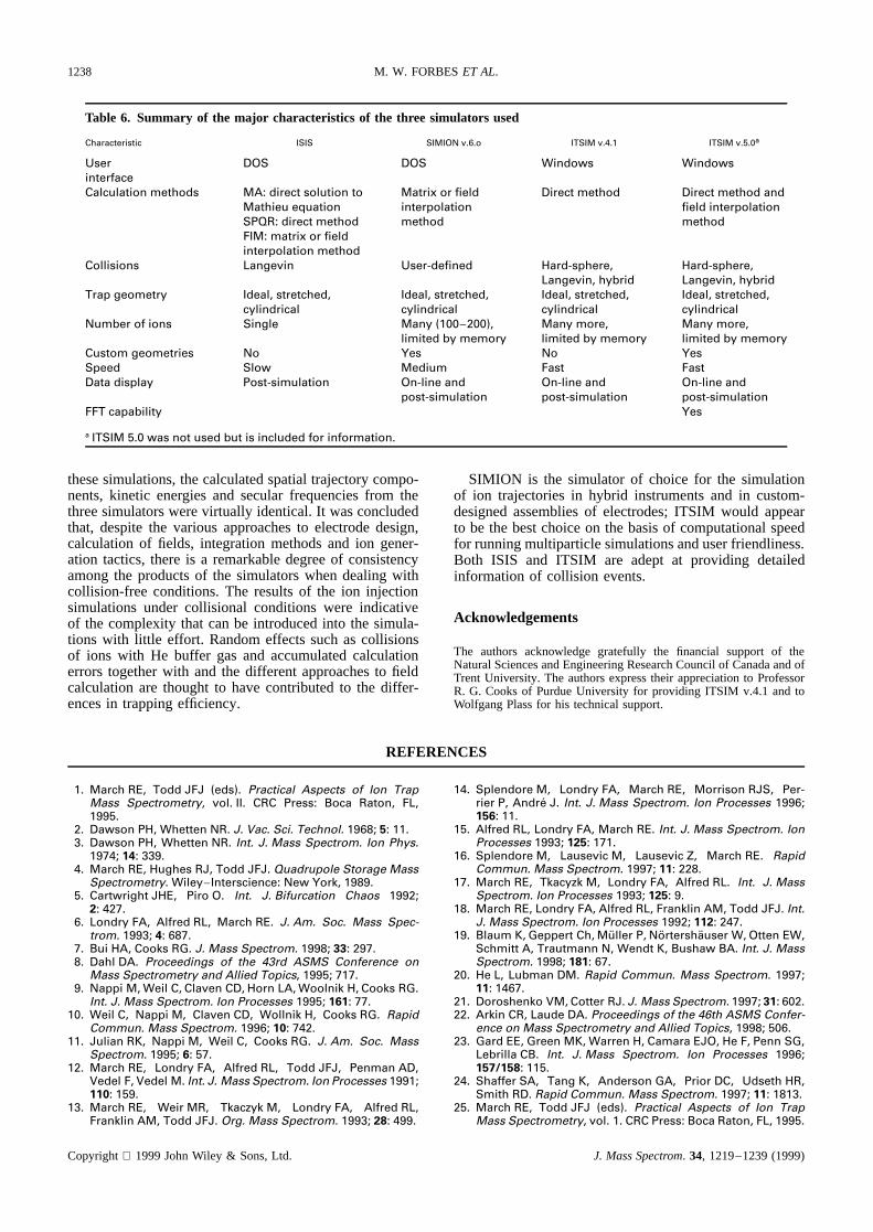
1238 M. W. FORBESET AL.
Table 6. Summary of the major characteristics of the three simulators used
Characteristic ISIS SIMION v.6.o ITSIM v.4.1 ITSIM v.5.0a
User DOS DOS Windows WindowsinterfaceCalculation methods MA: direct solution to
Mathieu equationSPQR: direct methodFIM: matrix or fieldinterpolation method
Matrix or fieldinterpolationmethod
Direct method Direct method andfield interpolationmethod
Collisions Langevin User-defined Hard-sphere,Langevin, hybrid
Hard-sphere,Langevin, hybrid
Trap geometry Ideal, stretched,cylindrical
Ideal, stretched,cylindrical
Ideal, stretched,cylindrical
Ideal, stretched,cylindrical
Number of ions Single Many (100 200),limited by memory
Many more,limited by memory
Many more,limited by memory
Custom geometries No Yes No YesSpeed Slow Medium Fast FastData display Post-simulation On-line and
post-simulationOn-line andpost-simulation
On-line andpost-simulation
FFT capability Yes
a ITSIM 5.0 was not used but is included for information.
these simulations, the calculated spatial trajectory compo-nents, kinetic energies and secular frequencies from thethree simulators were virtually identical. It was concludedthat, despite the various approaches to electrode design,calculation of fields, integration methods and ion gener-ation tactics, there is a remarkable degree of consistencyamong the products of the simulators when dealing withcollision-free conditions. The results of the ion injectionsimulations under collisional conditions were indicativeof the complexity that can be introduced into the simula-tions with little effort. Random effects such as collisionsof ions with He buffer gas and accumulated calculationerrors together with and the different approaches to fieldcalculation are thought to have contributed to the differ-ences in trapping efficiency.
SIMION is the simulator of choice for the simulationof ion trajectories in hybrid instruments and in custom-designed assemblies of electrodes; ITSIM would appearto be the best choice on the basis of computational speedfor running multiparticle simulations and user friendliness.Both ISIS and ITSIM are adept at providing detailedinformation of collision events.
Acknowledgements
The authors acknowledge gratefully the financial support of theNatural Sciences and Engineering Research Council of Canada and ofTrent University. The authors express their appreciation to ProfessorR. G. Cooks of Purdue University for providing ITSIM v.4.1 and toWolfgang Plass for his technical support.
REFERENCES
1. March RE, Todd JFJ (eds). Practical Aspects of Ion TrapMass Spectrometry, vol. II. CRC Press: Boca Raton, FL,1995.
2. Dawson PH, Whetten NR. J. Vac. Sci. Technol. 1968; 5: 11.3. Dawson PH, Whetten NR. Int. J. Mass Spectrom. Ion Phys.
1974; 14: 339.4. March RE, Hughes RJ, Todd JFJ. Quadrupole Storage Mass
Spectrometry. Wiley Interscience: New York, 1989.5. Cartwright JHE, Piro O. Int. J. Bifurcation Chaos 1992;
2: 427.6. Londry FA, Alfred RL, March RE. J. Am. Soc. Mass Spec-
trom. 1993; 4: 687.7. Bui HA, Cooks RG. J. Mass Spectrom. 1998; 33: 297.8. Dahl DA. Proceedings of the 43rd ASMS Conference on
Mass Spectrometry and Allied Topics, 1995; 717.9. Nappi M, Weil C, Claven CD, Horn LA, Woolnik H, Cooks RG.
Int. J. Mass Spectrom. Ion Processes 1995; 161: 77.10. Weil C, Nappi M, Claven CD, Wollnik H, Cooks RG. Rapid
Commun. Mass Spectrom. 1996; 10: 742.11. Julian RK, Nappi M, Weil C, Cooks RG. J. Am. Soc. Mass
Spectrom. 1995; 6: 57.12. March RE, Londry FA, Alfred RL, Todd JFJ, Penman AD,
Vedel F, Vedel M. Int. J. Mass Spectrom. Ion Processes 1991;110: 159.
13. March RE, Weir MR, Tkaczyk M, Londry FA, Alfred RL,Franklin AM, Todd JFJ. Org. Mass Spectrom. 1993; 28: 499.
14. Splendore M, Londry FA, March RE, Morrison RJS, Per-rier P, Andre J. Int. J. Mass Spectrom. Ion Processes 1996;156: 11.
15. Alfred RL, Londry FA, March RE. Int. J. Mass Spectrom. IonProcesses 1993; 125: 171.
16. Splendore M, Lausevic M, Lausevic Z, March RE. RapidCommun. Mass Spectrom. 1997; 11: 228.
17. March RE, Tkacyzk M, Londry FA, Alfred RL. Int. J. MassSpectrom. Ion Processes 1993; 125: 9.
18. March RE, Londry FA, Alfred RL, Franklin AM, Todd JFJ. Int.J. Mass Spectrom. Ion Processes 1992; 112: 247.
19. Blaum K, Geppert Ch, Muller P, Nortershauser W, Otten EW,Schmitt A, Trautmann N, Wendt K, Bushaw BA. Int. J. MassSpectrom. 1998; 181: 67.
20. He L, Lubman DM. Rapid Commun. Mass Spectrom. 1997;11: 1467.
21. Doroshenko VM, Cotter RJ. J. Mass Spectrom. 1997; 31: 602.22. Arkin CR, Laude DA. Proceedings of the 46th ASMS Confer-
ence on Mass Spectrometry and Allied Topics, 1998; 506.23. Gard EE, Green MK, Warren H, Camara EJO, He F, Penn SG,
Lebrilla CB. Int. J. Mass Spectrom. Ion Processes 1996;157/158: 115.
24. Shaffer SA, Tang K, Anderson GA, Prior DC, Udseth HR,Smith RD. Rapid Commun. Mass Spectrom. 1997; 11: 1813.
25. March RE, Todd JFJ (eds). Practical Aspects of Ion TrapMass Spectrometry, vol. 1. CRC Press: Boca Raton, FL, 1995.
Copyright 1999 John Wiley & Sons, Ltd. J. Mass Spectrom. 34, 1219–1239 (1999)

SIMULATION OF ION TRAJECTORIES IN A QUADRUPLE ION TRAP 1239
26. Knight RD. Int. J. Mass Spectrom. Ion Phys. 1983; 51: 127.27. March RE. J. Mass Spectrom. 1997; 32: 351.28. Mathieu E. J. Math. Pures Appl. 1868; 13: 137.29. Badman ER, Johnson RC, Plass WR, Cooks RG. Anal. Chem.
1998; 70: 4896.30. Wells JM, Plass WR, Patterson GE, Ouyang Z, Badman ER,
Cooks RG. Anal. Chem. 1999; 71: 3405.31. Wells JM, Plass WR, Patterson GE, Ouyang Z, Badman ER,
Cooks RG. In Proceedings of the 47th ASMS Confer-ence on Mass Spectrometry and Allied Topics, Dallas, TX,June 13 18, 1999; 568.
32. Dahl DA. SIMION 3D Version 6.0 User’s Manual. IdahoNational Engineering Laboratory Chemical Meterials andProcesses Department, Lockheed Idaho Technologies Com-pany: Idaho Falls, ID, 1995.
33. Bonner RF, Fulford JE, March RE. Int. J. Mass Spectrom. IonPhys. 1977; 24: 255.
34. Corson D, Lorrain P. Introduction to Electromagnetic Fieldsand Waves. W.H. Freeman: San Francisco, 1962; 36.
35. Cooks RG, Rockwood AL. Rapid Commun. Mass Spectrom.1991; 5: 93.
36. Atkins PW. Physical Chemistry, (2nd edn). Freeman & Co.,New York: 1994; 670.
37. Hemberger PH, Nogar NS, Williams JD, Cooks RG, SykaJEP. Chem. Phys. Lett. 1992; 191: 405.
38. Cleven CD, Cooks RG, Garrett AW, Nogar NS, Hem-berger PH. J. Phys. Chem. 1996; 100: 40.
39. Siemers I, Blatt R, Sauter T, Neuhauser W. Phys. Rev. A.1988; 38: 5121.
40. Guan S, Marshall AG. J. Am. Soc. Mass Spectrom. 1994;5: 64.
41. Paul W. Angew. Chem. Int. Ed. Engl. 1990; 29: 739.42. Gilbert RG. J. Chem. Phys. 1984; 80: 11.43. Mahan BH. J. Chem. Edu. C. 1974; 51: 308.44. Ho M. Honours Thesis, Trent University, Peterborough, ON,
1983.45. Moriwaki Y, Tachikawa M, Maeno Y, Shimizu T. Jpn. J. Appl.
Phys. 1992; 31: L1640.46. Cooks RG, personal communication.47. Quarmby ST, Yost RA. Int. J. Mass Spectrom. Ion Proc. 1999;
190/191: 81.48. Lide DR (ed). CRC Handbook of Chemistry and Physics, (75th
edn). CRC Press: Boca Raton, FL, 1995.49. Schlunegger UP, Stoeckli M, Caprioli RM. Rapid Commun.
Mass Spectrom. 1999; 13: 1792.
Copyright 1999 John Wiley & Sons, Ltd. J. Mass Spectrom. 34, 1219–1239 (1999)