Embed Size (px)
Citation preview
Accepted Manuscript
Title: Simulation of magnetic suspensions for HGMS usingCFD, FEM and DEM modeling
Author: <ce:author id="aut0005"> JohannesLindner<ce:author id="aut0010"> KatharinaMenzel<ce:author id="aut0015"> Hermann Nirschl
PII: S0098-1354(13)00077-XDOI: http://dx.doi.org/doi:10.1016/j.compchemeng.2013.03.012Reference: CACE 4669
To appear in: Computers and Chemical Engineering
Received date: 21-9-2012Revised date: 11-2-2013Accepted date: 11-3-2013
Please cite this article as: Lindner, J., Menzel, K., & Nirschl, H., Simulation of magneticsuspensions for HGMS using CFD, FEM and DEM modeling, Computers and ChemicalEngineering (2013), http://dx.doi.org/10.1016/j.compchemeng.2013.03.012
This is a PDF file of an unedited manuscript that has been accepted for publication.As a service to our customers we are providing this early version of the manuscript.The manuscript will undergo copyediting, typesetting, and review of the resulting proofbefore it is published in its final form. Please note that during the production processerrors may be discovered which could affect the content, and all legal disclaimers thatapply to the journal pertain.
Page 1 of 38
Accep
ted
Man
uscr
ipt
Simulation of magnetic particle movement using FEM and CFD Page 1
Simulation of magnetic suspensions for1
HGMS using CFD, FEM and DEM modeling2
Johannes Lindner, Katharina Menzel, Hermann Nirschl3
Institute of Mechanical Process Engineering and Mechanics, Karlsruhe Institute of Technology, Germany4
[email protected]; [email protected]
Phone: 0049/721/608-42427; Fax: 0049/721/608-424036
Abstract7
Properties of magnetic suspensions depend on the fluid, the particles and the magnetic background field. 8
The simulation is aimed at understanding the influence of magnetic properties in High Gradient Magnetic 9
Separation processes. In HGMS magnetic particles are collected on magnetic wires for separation. External 10
magnetic forces are calculated or simulated using the Finite Element Method and embedded first in a 11
Computational Fluid Dynamics simulation. In the simulation, elliptic and rectangular wires aligned in field 12
direction reach higher separation efficiencies than cylindrical wires. Magnetic forces from FEM with13
implemented dipole forces in a Discrete Element Method code show magnetically induced agglomeration 14
and yield an acceptable agreement with experiments. Particle deposition on wires is investigated under the 15
influence of different parameters. The porosity of the deposit is dependent on the magnetization of the 16
wire and particles. A centrifugal force of 60 g has an important influence. 17
Highlights18
Finite Element Modeling simulation read in Computational Fluid Dynamics for magnetic particle 19
tracks20
Discrete Element Modeling of magnetic particle chains21
Page 2 of 38
Accep
ted
Man
uscr
ipt
Simulation of magnetic particle movement using FEM and CFD Page 2
Simulation of magnetic fluids 22
Keywords: CFD, DEM, FEM, HGMS, particle process23
1. Introduction24
The viscosity of magnetic suspensions is highly anisotropic and can be set externally by changing the 25
magnetic field [1]. It is therefore interesting to simulate the behavior of magnetic suspensions for a 26
better understanding of particle agglomerate porosity and shape, particle motion during separation, 27
the possibility of particle displacement in the magnetic field under centrifugal force, and the 28
separation of particles by magnetic forces to wires of rectangular shape. The separation efficiency of 29
wires is necessary for an optimization of the specific High Gradient Magnetic Separation (HGMS) 30
process. 31
HGMS has been used for many years to remove magnetic solids from fluid flow. It has become a 32
standard method since its invention in 1937 by Frantz. Usually, the particles are separated by wires in 33
the fluid, which are magnetized by an external magnetic field [2]. An application is the use of 34
functionalized particles with a magnetic core in downstream processing of biotechnological processes.35
Eichholz et al. separated lysozyme from hen egg white by magnetic cake filtration [3]. HGMS is applied 36
in wastewater treatment [2] or for the separation of ferrous contaminants from oil [4]. 37
The aim is the simulation of the HGMS process. Using existing equations, it is possible to calculate the 38
magnetic force acting on a particle and, hence, the particle flow in Computational Fluid Dynamics 39
(CFD) [5]. Okada et al. used CFD simulation to determine the separation efficiency of different wire 40
arrangements [6]. Hournkumnuard et al. used a Finite Difference Method to simulate concentration 41
distributions [7]. Elliptic wire shapes were investigated by Li et al. [8].42
Analytical approaches are limited to elliptical geometries. While round geometries are used in many 43
applications, another shape of the separating device is chosen in some cases. Hayashi et al. [9]44
simulated the magnetic field and the fluid using Finite Element Modeling (FEM) and calculated the 45

Page 3 of 38
Accep
ted
Man
uscr
ipt
Simulation of magnetic particle movement using FEM and CFD Page 3
particle trajectory by solving the equation of motion for a rectangular wire shape. From this, they 46
deduced the particle capture area in their specific experiment. An example of the use of different wire 47
shapes is Magnetically Enhanced Centrifugation (MEC) [9]: the separating device is structured by laser 48
cutting, resulting in a rectangular shape. The investigation of this shape and its influence on separation 49
is in the focus of this article. The reason for creating structured wires lies in the process itself: in MEC 50
the wire is cleaned by centrifugation during magnetic filtration. This allows in theory for a continuous 51
process. The magnetic forces extend the time magnetic particles stay in the centrifuge by capturing 52
them on a wire. Particles agglomerate on the wire and upper layers are removed by centrifugation. 53
This requires star-shaped matrices which are produced most easily by laser cutting. CFD simulations of 54
centrifuges have already been made, particle tracks in centrifuges have already been calculated [10, 55
11]. 56
In this paper the magnetic field is modeled by FEM simulation. Fluid flow is simulated by CFD using a 57
finite volume grid. The magnetic field is read into the CFD grid to determine the magnetic and fluid 58
forces acting on a particle at each position. In comparison to the common analytical calculation, the 59
advantage of this method lies in the fact that any geometry of a magnetic field can be calculated. In 60
particular, it is possible to calculate magnetic wires of irregular shape as well as wires that are located 61
too closely to each other for a simple addition of the magnetic forces. 62
Understanding of particle agglomerate building allows comprehension of different effects we face in 63
the process such as strongly changing porosity under different conditions, notably different field 64
strength or particle remanence. Another important effect is the particular deposit shape on magnetic 65
wires. Satoh [12] studied ferromagnetic colloidal dispersions of clusters of ferromagnetic particles. The 66
same formulae are now used in this paper to simulate interparticle forces. Fei Chen simulated 67
magnetic deposit on wires using the Discrete Element Method (DEM) in a 2D approach [13]. DEM is 68
used to simulate interparticle forces and agglomeration. A review on DEM is given in [14, 15]. 69
Magnetic forces between particles are simulated analytically. Deposition of particles on a wire was 70

Page 4 of 38
Accep
ted
Man
uscr
ipt
Simulation of magnetic particle movement using FEM and CFD Page 4
simulated based on an analytical solution for the wire force acting on particles or a FEM vector field 71
read into the DEM simulation. Numeric simulation is the only way to investigate the behavior of 72
particles in an irregular magnetic field created at wire edges. The present paper focuses on the 73
simulation of magnetic particles in general and in combination with centrifuges. An overview over 74
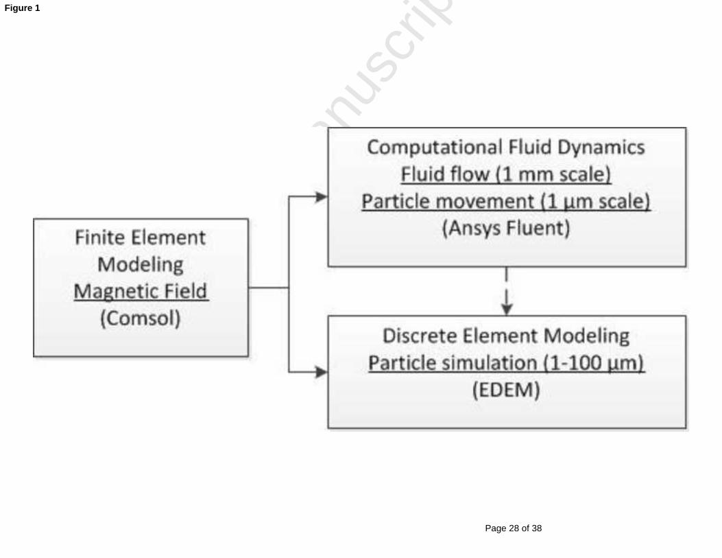
simulation approaches and information flow is given in Figure 1. 75
Figure 1: Simulation methods and scale76
2. Theory77
We read magnetic fields simulated by FEM into a CFD simulation, and into a DEM simulation. For the 78
latter several assumptions and simplifications were taken in our modeling approach of the Discrete 79
Element Model:80
1. Magnetic particles may be approached by a magnetic dipole despite not having an infinitesimal 81
small core.82
2. The approximation of the field around more than one dipole is not exact, as they interfere and 83
soften or strengthen each other’s magnetic field. We only took into account the direct 84
neighboring particle in particle chains, which is physically not correct yet showed to be 85
necessary to achieve a stable simulation.86
3. Influence of hydrodynamic forces change kinetics but not final particle deposit shape and 87
stability to centrifugal forces.88
4. Surface forces including capillary forces may be neglected. This results for the investigated 89
particle sizes of a force comparison. 90
5. Magnetic matter distorts the field. However to simplify the model, we assume magnetic 91
particles to be aligned in direction of the external field. 92
Page 5 of 38
Accep
ted
Man
uscr
ipt
Simulation of magnetic particle movement using FEM and CFD Page 5
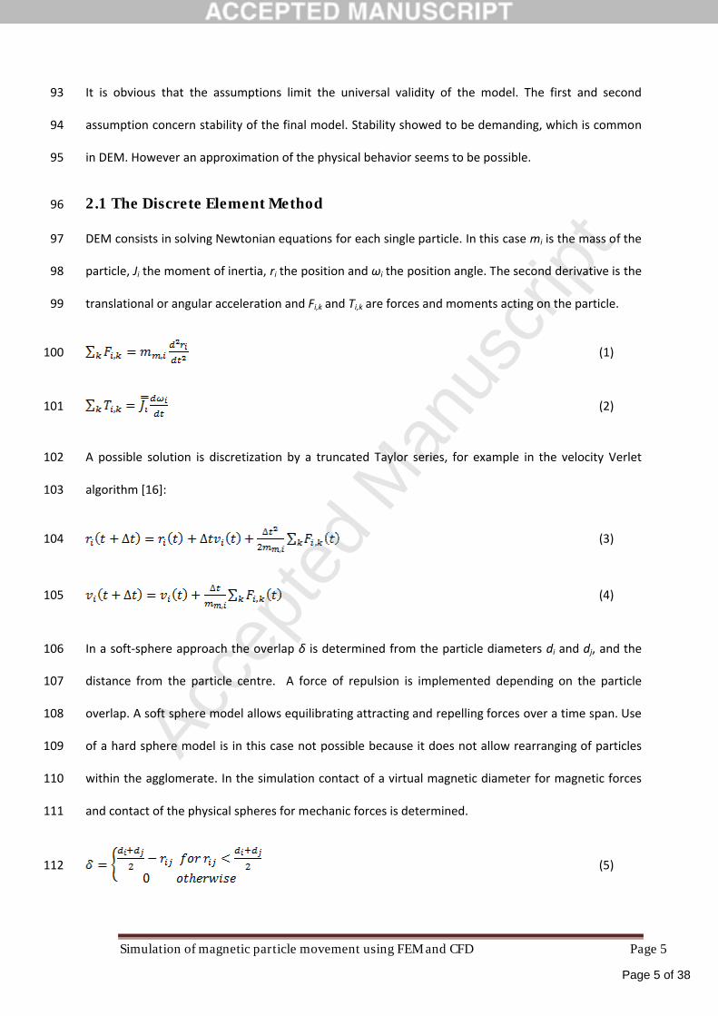
It is obvious that the assumptions limit the universal validity of the model. The first and second 93
assumption concern stability of the final model. Stability showed to be demanding, which is common 94
in DEM. However an approximation of the physical behavior seems to be possible. 95
2.1 The Discrete Element Method96
DEM consists in solving Newtonian equations for each single particle. In this case mi is the mass of the 97
particle, Ji the moment of inertia, ri the position and ωi the position angle. The second derivative is the 98
translational or angular acceleration and Fi,k and Ti,k are forces and moments acting on the particle. 99
(1)100
(2)101
A possible solution is discretization by a truncated Taylor series, for example in the velocity Verlet 102
algorithm [16]:103
(3)104
(4)105
In a soft-sphere approach the overlap δ is determined from the particle diameters di and dj, and the 106
distance from the particle centre. A force of repulsion is implemented depending on the particle 107
overlap. A soft sphere model allows equilibrating attracting and repelling forces over a time span. Use 108
of a hard sphere model is in this case not possible because it does not allow rearranging of particles 109
within the agglomerate. In the simulation contact of a virtual magnetic diameter for magnetic forces 110
and contact of the physical spheres for mechanic forces is determined. 111
(5)112
Page 6 of 38
Accep
ted
Man
uscr
ipt
Simulation of magnetic particle movement using FEM and CFD Page 6
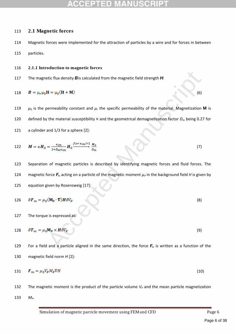
2.1 Magnetic forces113
Magnetic forces were implemented for the attraction of particles by a wire and for forces in between 114
particles. 115
2.1.1 Introduction to magnetic forces116
The magnetic flux density B is calculated from the magnetic field strength H: 117
(6)118
µ0 is the permeability constant and µr the specific permeability of the material. Magnetization M is 119
defined by the material susceptibility and the geometrical demagnetization factor Dm being 0.27 for 120
a cylinder and 1/3 for a sphere [2]: 121
(7)122
Separation of magnetic particles is described by identifying magnetic forces and fluid forces. The 123
magnetic force Fm acting on a particle of the magnetic moment µP in the background field H is given by 124
equation given by Rosensweig [17]: 125
(8)126
The torque is expressed as: 127
(9)128
For a field and a particle aligned in the same direction, the force Fm is written as a function of the 129
magnetic field norm H [2]:130
(10)131
The magnetic moment is the product of the particle volume VP and the mean particle magnetization 132
MP. 133
Page 7 of 38
Accep
ted
Man
uscr
ipt
Simulation of magnetic particle movement using FEM and CFD Page 7
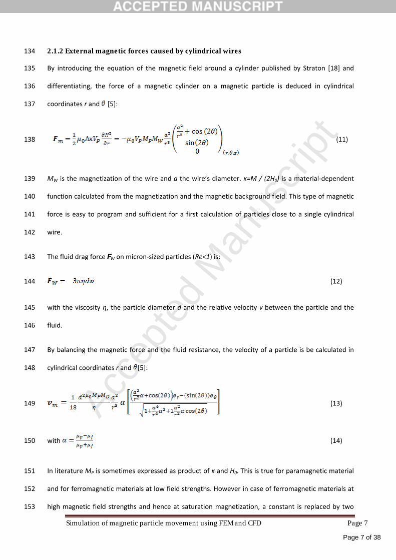
2.1.2 External magnetic forces caused by cylindrical wires134
By introducing the equation of the magnetic field around a cylinder published by Straton [18] and 135
differentiating, the force of a magnetic cylinder on a magnetic particle is deduced in cylindrical 136
coordinates r and [5]:137
(11)138
MW is the magnetization of the wire and a the wire’s diameter. κ=M / (2H0) is a material-dependent 139
function calculated from the magnetization and the magnetic background field. This type of magnetic 140
force is easy to program and sufficient for a first calculation of particles close to a single cylindrical 141
wire. 142
The fluid drag force FW on micron-sized particles (Re<1) is: 143
(12)144
with the viscosity η, the particle diameter d and the relative velocity v between the particle and the 145
fluid. 146
By balancing the magnetic force and the fluid resistance, the velocity of a particle is be calculated in 147
cylindrical coordinates r and [5]: 148
(13)149
with (14)150
In literature MP is sometimes expressed as product of κ and H0. This is true for paramagnetic material 151
and for ferromagnetic materials at low field strengths. However in case of ferromagnetic materials at 152
high magnetic field strengths and hence at saturation magnetization, a constant is replaced by two 153
Page 8 of 38
Accep
ted
Man
uscr
ipt
Simulation of magnetic particle movement using FEM and CFD Page 8
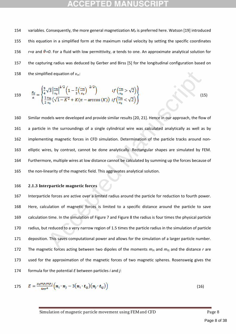
variables. Consequently, the more general magnetization MP is preferred here. Watson [19] introduced 154
this equation in a simplified form at the maximum radial velocity by setting the specific coordinates 155
r=a and =0. For a fluid with low permittivity, α tends to one. An approximate analytical solution for 156
the capturing radius was deduced by Gerber and Birss [5] for the longitudinal configuration based on 157
the simplified equation of vm: 158
(15)159
Similar models were developed and provide similar results [20, 21]. Hence in our approach, the flow of 160
a particle in the surroundings of a single cylindrical wire was calculated analytically as well as by 161
implementing magnetic forces in CFD simulation. Determination of the particle tracks around non-162
elliptic wires, by contrast, cannot be done analytically. Rectangular shapes are simulated by FEM. 163
Furthermore, multiple wires at low distance cannot be calculated by summing up the forces because of 164
the non-linearity of the magnetic field. This aggravates analytical solution. 165
2.1.3 Interparticle magnetic forces166
Interparticle forces are active over a limited radius around the particle for reduction to fourth power. 167
Here, calculation of magnetic forces is limited to a specific distance around the particle to save 168
calculation time. In the simulation of Figure 7 and Figure 8 the radius is four times the physical particle 169
radius, but reduced to a very narrow region of 1.5 times the particle radius in the simulation of particle 170
deposition. This saves computational power and allows for the simulation of a larger particle number. 171
The magnetic forces acting between two dipoles of the moments mPi and mPj and the distance r are 172
used for the approximation of the magnetic forces of two magnetic spheres. Rosensweig gives the 173
formula for the potential E between particles i and j: 174
(16)175
Page 9 of 38
Accep
ted
Man
uscr
ipt
Simulation of magnetic particle movement using FEM and CFD Page 9
The potential depends on the orientation of the magnetic particle moments ni and nj relative to each 176
other and to the vector from particle i to j tij. The formula was evaluated by Satoh [12] for the force 177
Fm,ij: 178
179
(17)180
The moment Tm,ij on a magnetic particle is: 181
(18)182
Now, the magnetic particles are assumed to be directed in field direction. The Cartesian product in the 183
same direction is zero. Hence, the moments resulting from both different particles and the magnetic 184
field are neglected. The force was simplified under the assumption of the particles being aligned in x-185
direction of a constant magnetic field with the components of the direction vector tx, ty and tz:186
(19)187
Under the same assumption of aligned particles, torsion is neglected in this simulation. 188
2.2 Non-magnetic forces189
2.2.1 Mechanic forces190
The mechanic interparticle forces were introduced by Mindlin. In our case, the mechanical forces 191
counteract attracting magnetic forces and allow for a stable equilibrium to simulate magnetically 192
induced agglomeration. Mechanical forces are divided into spring and damper forces. The spring force 193
and damper force in normal direction Fn,ij are as follows [22-24]: 194
(20)195
Page 10 of 38
Accep
ted
Man
uscr
ipt
Simulation of magnetic particle movement using FEM and CFD Page 10
with (21)196
and (22)197
The material parameters, spring constant kn and the damper constant ηn,ij, are difficult to determine in 198
the case of µm-sized particles. Hence, they are calculated from material properties. However, the 199
overlap δ adapts to achieve equilibrium, which results in magnetic agglomeration independently of 200
particle stiffness. The tangential damper force is: 201
(23)202
with (24)203
with cn=0.3 [25]. This force is necessary to prevent oscillation of one particle around the region of 204
highest magnetic field of another particle. The coefficients have been chosen according to [26]. Flow 205
resistance of a single particle in a laminar regime according to Stokes is given in (6). A summary of 206
DLVO forces introduced in [27] did not show significant differences in the simulation. 207
2.2.2 The centrifugal force208
Magnetically enhanced centrifugation is an important use of the simulation. The influence of the wire 209
force is simulated to identify possibilities to clean the wire. The centrifugal force FZ is implemented as 210
constant acceleration in wire direction. The centrifugal force at the wire end is implemented for the 211
whole simulation area as constant r for simplicity. It is calculated from centrifugal velocity ω. 212
(25)213
Centrifugal force is normalized to the gravitational force to eliminate units:214
(26)215
Page 11 of 38
Accep
ted
Man
uscr
ipt
Simulation of magnetic particle movement using FEM and CFD Page 11
3. Simulation methods216
3.1 Methods to simulate magnetic wire forces217
Simulation of the magnetic field by FEM218
Particle separation was simulated from wires of elliptic and rectangular shape of the same cross 219
section area but different semi-axis. For this purpose the magnetic field was determined by FEM220
(Comsol Version 3.4) and read into a CFD code to calculate forces on particles. The permeability was 221
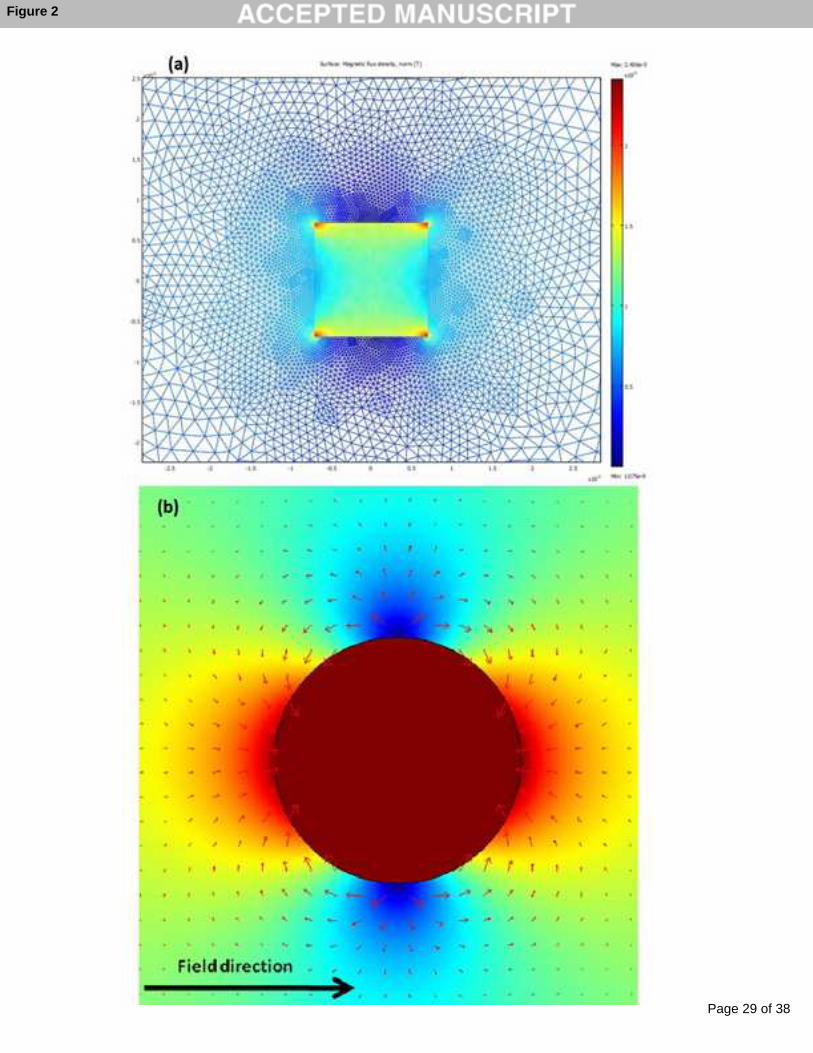
set to 1 for the fluid and 5 for the wire at the background field of 400 kA/m corresponding 0.5 T. Figure 222
2 (a) shows the FEM grid and the magnetic field around a rectangular wire. The corners of the 223
rectangle are prone to numerical errors, which is limited to a very small area by a fine grid. 224
Figure 2: The FEM grid around a rectangular wire (a); the field and field gradient around a cylindrical wire (b)225
Figure 2 (b) shows the field around a cylindrical wire. The colors indicate the field strength; there is a 226
maximum in the horizontal field direction and a minimum perpendicular to the field direction. The 227
resulting gradient is shown by the arrows. The field is attractive in background field direction left and 228
right and repulsing perpendicular to the field. The gradient was calculated and then exported with the 229
coordinates of each node. 230
Implementation of the magnetic forces in CFD231
Ansys Fluent Version 12 was used to simulate the fluid flow around wires of different shape. The field 232
gradient was read into Fluent. The node value of the magnetic field gradient in x and y direction was 233
read into a CFD code and stored in the memory of the finite volume cells by assigning the closest 234
value. An interpolation seemed not to be necessary by having sufficiently fine grids. The particle tracks 235
of different wires were simulated using this approach. As discretization causes inaccuracies, the finite 236
volume grid has to be fine near the wire similarly to the finite element grid. After simulation of the 237
fluid flow the force on the particles was calculated from eq. (10) at discrete time steps. Fluid velocity is 238
Page 12 of 38
Accep
ted
Man
uscr
ipt
Simulation of magnetic particle movement using FEM and CFD Page 12
1 mm/s, which is the same scale as in our HGMS experiments. Particle magnetization in this case is 239
1.26e6 A/m. This led to particle tracks around wires, which reflected the separation of particles. 240
3.2 Methods to simulate interparticle forces by DEM241
The computer system used was Windows XP SP2. The computer was a quad core with 3.14 GHz, 64 bit 242
and 8 GB Ram. As function implementation did not allow parallel simulation, simulations were 243
performed on a single core. The software EDEM Version 2.3.1 of DEM Solutions was used as 244
framework and for graphical view. The magnetic forces as well as the mechanic contact model were 245
programmed in C and implemented in the simulation as user-defined library (UDL). Windows SDK 7.1 246
was used to compile the source code. Eq. (11) was implemented to simulate the force of the magnetic 247
wire on the particles, except for simulations implementing the centrifugal force. To simulate the field 248
on the wire end on centrifugal force influence, the magnetic field was read and implemented using eq 249
(10). In the contact model, eq. (19) was implemented as the magnetic model. The mechanic model 250
consisted of eqs. (20) and (23) with the parameters of eqs. (21), (22) and (24). As mentioned in the 251
second assumption, magnetic forces were suppressed for distant particles in the same agglomerate. 252
This eliminated instabilities, specifically particles in the middle of the wire being pushed out by 253
neighboring particles. We suppose this instability to be consequence of the approximation of the 254
magnetic particle core with a dipole equation (17) and the superposition of magnetic forces. Important 255
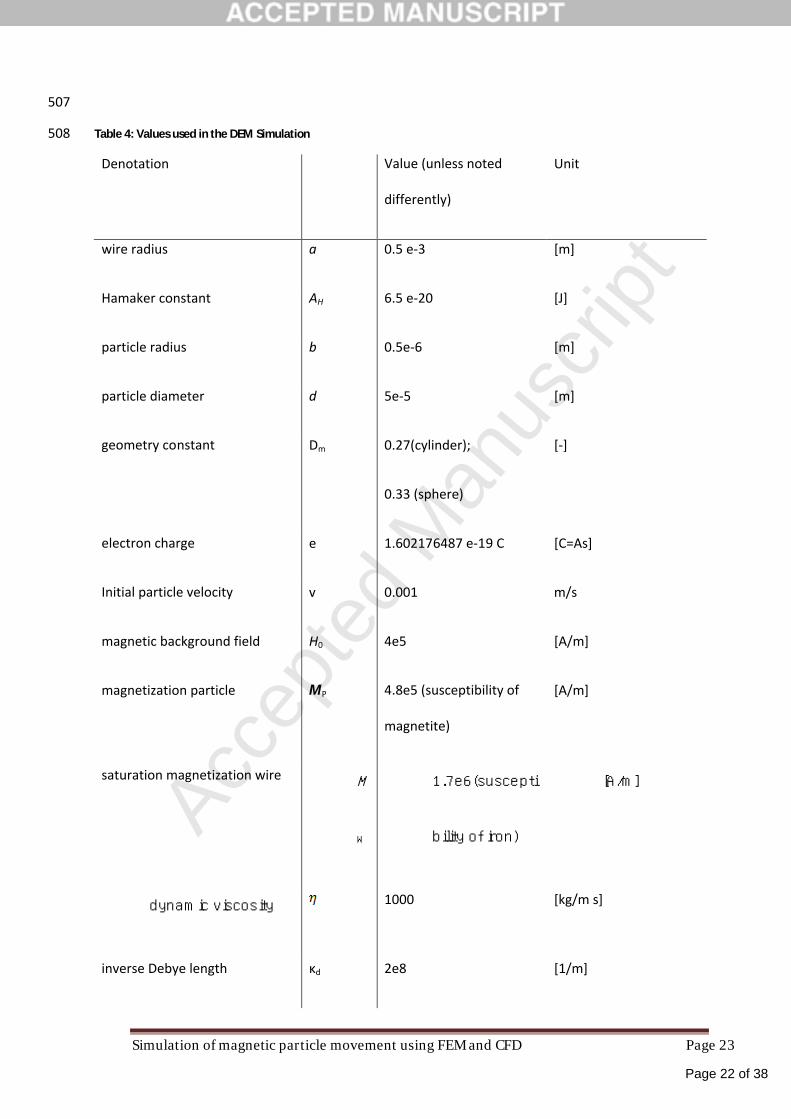
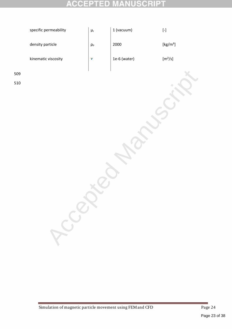
values in the DEM simulation are given in Table 1. 256
Table 1: Values used in the DEM Simulation257
Interparticle forces summarized in the DLVO theory usually are only important for particle sizes below 258
µm-scale. According to [27] magnetic forces predominate over surface forces for the particle sizes 259
simulated. A simulation, including the DLVO theory and fluid flow summarized in [27], was performed 260
for particles of 1 µm in size, yet did not change the final shape of the deposit, hence DVLO and CFD 261
forces were neglected in further simulations. 262
Experimental Validation263
Page 13 of 38
Accep
ted
Man
uscr
ipt
Simulation of magnetic particle movement using FEM and CFD Page 13
Validation is necessary to reveal shortcomings which are inevitable in every model or simulation. We 264
decided to compare the deposit of magnetite particles on a ferrous wire in a magnetic field in air by 265
pouring a small amount of particles over a wire in a magnetic field (see 4.2.1 Validation). The process 266
of deposition could not be visualized in an experiment due to the low medium particle size of 2 µm 267
and the high velocities during deposition in the range of several m/s. In comparison the time scale of 268
the simulation was 50 ms. Simulation time itself was about 10 h. For particle deposition, a wire of 1 269
mm in diameter and 25 mm in length was used. The wire material was a ferromagnetic steel with the 270
material number 1.4016 with a saturation magnetization of 1.3 * 106 A/m. The particles were iron 271
oxide particles, named Bayoxid 8706, with a saturation magnetization of about 400 000 A/m.272
4. Results and discussion273
4.1 Results and discussion of FEM and CFD coupling274
Birss et al. [28] give a formula for the attractive angle θc for cylindrical geometry. The angle specifies 275
the limit between the attractive and the repelling zone on the wire surface: 276
(27)277
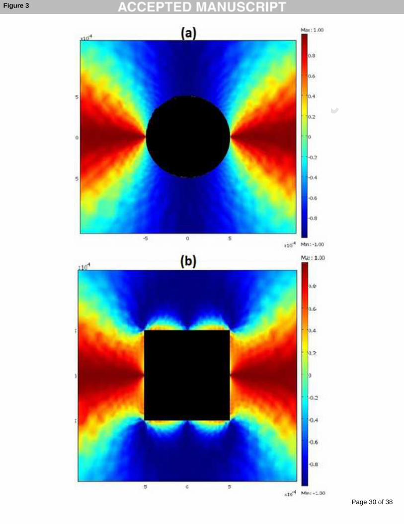
For an elliptic geometry, decreases from 90° to 45° with rising r, the value of the force being very 278
low at high distance. In a rectangular geometry, the angle determined in the simulation is 0° close to 279
the wire and approaches 45° at high distance. 280
Figure 3: The radial field component versus the normalized field force Fr/|F| for a cylindrical (a) and rectangular (b) wire 281
shape282
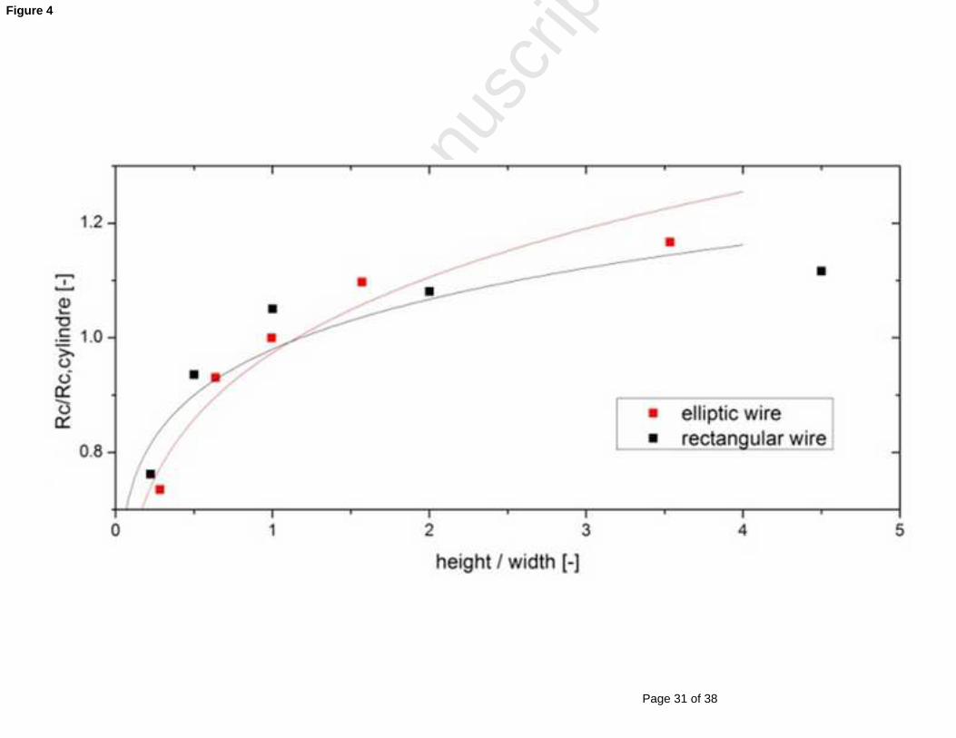
As seen in Figure 4, the capturing radius was normalized to the radius of a cylindrical wire for different 283
ratios of height h to width i. The capturing radius may be approximated by a simple power function. 284
The form of the function is: 285
Page 14 of 38
Accep
ted
Man
uscr
ipt
Simulation of magnetic particle movement using FEM and CFD Page 14
(28)286
Rc is the capturing radius of the wire to be calculated and Rc,cylinder the capturing radius of a wire of the 287
same area, which was calculated by the formulae of Gerber/Birrs [5], Uchiyama/Hayashi [21] or Cowen288
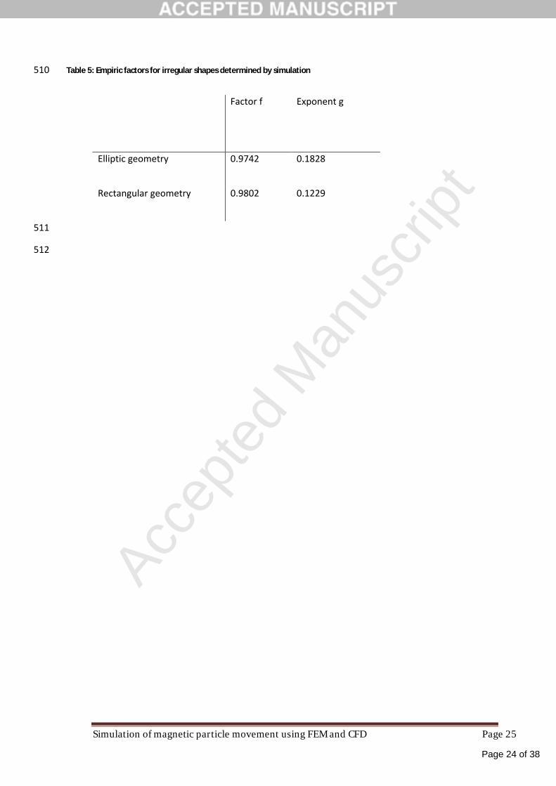
[20]. The simulation suggests the following parameters for rectangular and elliptic geometries to 289
approximate rectangular and elliptic shaped wires shown in Table 2. 290
Table 2: Empiric factors for irregular shapes determined by simulation291
Figure 4: Capture radius of different wire shapes normalized to the cylindrical wire's capture radius plotted versus the 292
relation length/width293
As evident from Figure 4, the power function is an approximation. The lower capturing radius for a 294
quadratic wire shape might be due to smaller gradients for a slightly unfavorable geometry as well as 295
to a disadvantageous fluid flow around the wire compared to the more elongated geometries in fluid 296
direction. Nevertheless, the formula represents an acceptable approximation for calculation purposes. 297
The result is in line with experiments, showing that wire shapes arranged parallel to the field direction 298
enhance separation slightly [29]. 299
A wire of quadratic shape of specific edge length seemed to have a higher capturing radius than a 300
cylindrical wire having a diameter corresponding to the edge length. Compared to the simulation, this 301
seems to be primarily due to the fact that the quadratic wire has a larger cross-sectional area and, 302
hence, higher mass rather than an effectively better geometry. In the simulation the advantage of the 303
field gradient seems to be compensated by disadvantages in the flow.304
As an outlook, the simulation size is limited by the assignment of FEM node values to VFM cell values. 305
The number of operations is the product of the numbers of FEM nodes and FVM cells. Hence, for very 306
large grids, the reading procedure is extended dramatically, complicating 3-dimensional simulation. To 307
improve the simulation, an approach performing both simulations on a single grid seems to be the best 308
way to handle 3-dimensional geometries. 309
Page 15 of 38
Accep
ted
Man
uscr
ipt
Simulation of magnetic particle movement using FEM and CFD Page 15
4.2 Results and discussion of the DEM model310
Simulation of particle trajectories is not sufficient to describe the behavior of magnetic suspensions 311
due to the influence of particles on each other. Experiments show needle-shaped magnetically induced 312
agglomeration of particles. Velocities of particles in the vacuum are high and strongly reduced when 313
the drag model is implemented. The same behavior appears in the simulation. The attraction zones 314
simulated in the FEM model allow for particle agglomeration only on the two sides of a particle aligned 315
in field direction (see Figure 2). 316
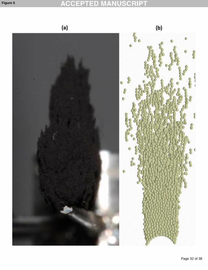
4.2.1 Validation317
For experimental validation, a small amount of particles was poured over the wire, resulting in the 318
deposit shown in Figure 5 (a). The medium particle diameter was 2 µm, as was measured by laser 319
diffraction. Figure 5 (b) shows a simulation based on 100 µm particles. The final image looks similar, 320
despite the different particle size. A simulation close to the real particle size was not possible due to 321
the huge particle amount necessary. In the simulation 500 particles were simulated. 322
The most obvious difference is the circular deposit in the experiment compared to the simulation. The 323
reason is the change of the field direction of the wire which we neglected due to assumption 5. This 324
was necessary so the model could be simplified in eq. (19). To avoid this inaccuracy in a future 325
simulation, particle rotation has to be permitted and the field direction change of wire and 326
surrounding particles has to be implemented based on equations (17) and (18). This results in a more 327
sophisticated and computationally expensive model. The shape of the deposit, densely packed close to 328
the wire and porous in upper layers, is in the simulation in good agreement with the experiment. 329
Figure 5: Agglomeration of Bayoxid particles on a wire (a) and simulation of 100 µm particles on a 1 mm wire (b)330
Comparison with other simulations331
Our simulation shall now be compared with a simulation of other researchers. For comparison, we 332
plotted an image published by Fei Chen [13]. He simulated the influence of centrifugal force on particle 333
Page 16 of 38
Accep
ted
Man
uscr
ipt
Simulation of magnetic particle movement using FEM and CFD Page 16
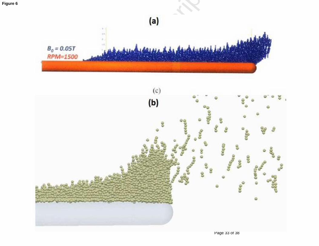
deposition. A similar simulation is explained in detail and compared with the simulation in Figure 10. 334
Acceleration was calculated from the rotational velocity of 1500 rpm as 60 g. The simulation was done 335
in 2D contrary to our simulation in Figure 10. Agreement of Figure 6 (a) and Figure 6 (b) was not ideal336
at the end of the wire. In our simulation, there are no particles beyond the end of the wire. This 337
difference may be caused by a difference in the simulation of the magnetic field by FEM. The magnetic 338
field resulting from our simulation had a steep decline at the end, resulting in huge repelling forces 339
from this zone towards the wire on the left as well as towards the right at the right end of the zone. 340
The steep end of the deposit at the wire end of Figure 6 (b) was due to the repelling forces of magnetic 341
particles on each other perpendicular to the magnetic field, see Figure 3 (a). However, this was the 342
only major difference to the Figure 6 (a). 343
Figure 6: 2D simulation of Fei Chen [13] (a); image of a simulation at 60 g for comparison (b)344
4.2.2 Simulation results345
Agglomeration346
Interparticle agglomeration is an important aspect in the simulation of magnetic suspensions. The 347
rheological behavior of particles as well as their settling velocity on a magnet depend to our 348
knowledge on agglomeration. Hence, this element is important for the understanding of particle 349
separation and its simulation is necessary for an accurate representation. Needle-shaped 350
agglomeration is documented in literature [30]. A simulation implementing one large particle showed 351
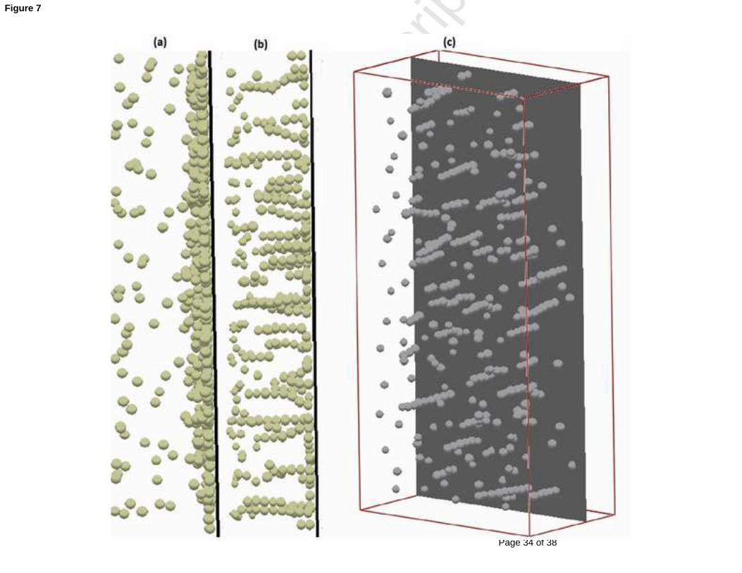
agglomeration of 100 µm particles on the surface of a significantly larger 1 mm particle (Figure 7). The 352
characteristic needle-shaped deposit was visible in this simulation. Particles agglomerated in particular 353
at one end of the large particle and formed needles. More important than the agglomeration on the 354
large particle is the agglomeration of monodisperse particles. 355
Figure 7: Particle agglomeration of 100 µm particles near one 1 mm particle356
Wire deposit357
Page 17 of 38
Accep
ted
Man
uscr
ipt
Simulation of magnetic particle movement using FEM and CFD Page 17
Usually, magnetic wires are made of ferromagnetic steel, while the particles have a magnetite core. 358
The magnetization of the wire is far higher than the magnetization of the particles. However, in case of 359
larger particle magnetization or at a large distance from the wire, the shape and porosity of the 360
agglomerate changed significantly in our simulation. For comparison, we simulated different 361
magnetizations to show the influence on the cake structure. 362
The magnetic force of a wire was implemented in this simulation. In combination with the interparticle363
forces, the particle deposit on a wire was simulated. The simulation showed a needle-shaped or a 364
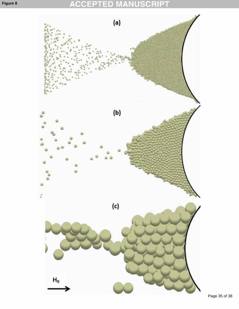
dense particle cake, depending on the magnetization of the wire to that of the particle. In Figure 8 (a), 365
a dense particle deposit is shown. In Figure 8 (b) and (c), the magnetization of the wire was reduced by 366
a factor 70 from the value determined for the wire material. The shape of the deposit was different, 367
showing a highly porous needle-shaped structure. It seems logical that the deposit depends on the 368
ratio of the magnetic wire force and the interparticle force. 369
Figure 8: Agglomerates of 1 µm particles on an iron wire (a) and on a weakly magnetic wire (b), (c)370
Size comparison of particles on a wire371
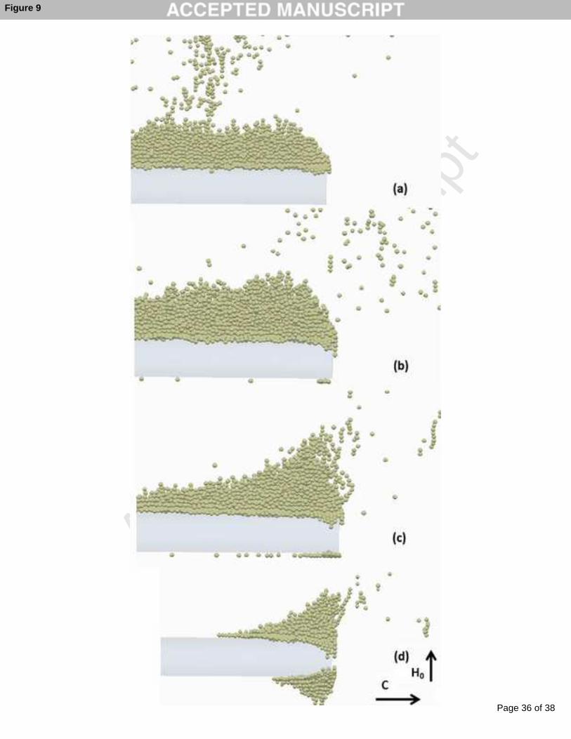
A simulation on different particle sizes was performed (Figure 9). The deposit of 10 µm particles (a) 372
and 20 µm particles (b) is virtually identical. For 100 µm particles (c), the deposit was similar. We 373
expected this result out of the implemented equations. Due to these similarities, the size difference is 374
not expected to be important in the validation. The final shape seems to be more dependent on 375
different parameters like particle magnetization than on the particle size. 376
Figure 9: Comparison of particles of different sizes: 10 µm (a); 20 µm (b); 100 µm (c)377
Influence of centrifugal force on wire deposit378
The simulation of the magnetic field at the wire end by FEM allows calculating the sliding of particles 379
under a gravitational or centrifugal field. This is important to simulate the behavior of particles in 380
superposed centrifugation and magnetic separation. Magnetically enhanced centrifugation, which is 381
Page 18 of 38
Accep
ted
Man
uscr
ipt
Simulation of magnetic particle movement using FEM and CFD Page 18
one of our research areas, is used for the simultaneous separation and cleaning of a magnetic wire 382
filter. In the centrifuge the height of the deposit depends on the centrifugal force. Centrifugal force is 383
used to structure the deposit. The amount of particles caught on the wire depends as well on the 384
centrifugal force. In the experiment the shape of the cake on the wire was uniform in the direction of 385
the wire axis. 386
For this geometry, large gradients created high forces at the end, which retained the particles. In 387
Figure 10 the wire simulation is shown for a field in vertical direction. The particle needles were 388
aligned in field direction. A centrifugal force of 0, 10, 60 and 240 g, respectively, was applied. In this 389
case, magnetic forces and friction counteracted centrifugal forces. The deposit slid to the outside in 390
comparison with a uniform distribution without centrifugal force. Accuracy might be limited by the 391
way forces are calculated (see assumption 2). 392
Figure 10: Magnetic field at the end of a wire simulated in FEM. Comparison of a wire end at 0 g (a), 10 g (b), 60 g (c) and 393
240 g (d).394
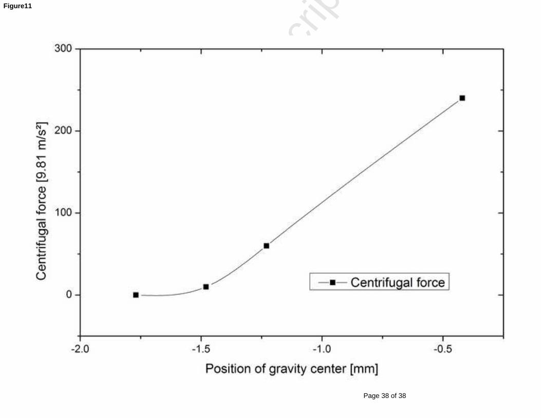
The centre of gravity of the particle deposit in the simulation moved to the outside, which is shown in 395
Figure 11. At 240 g, particles were mainly retained on the wire by the large gradients at the wire end. 396
Hence, the particle centre of gravity was very close to the end. The large gradient at the wire end was 397
the reason for the large displacement of the centre of gravity. 398
Figure 11: Diagram of the movement of the centre of gravity399
Wire shape400
Rectangular wires behaved similar to cylindrical wires in both experiment and simulation regarding the 401
structure of the particle deposit, as well under centrifugal forces. However simulation of a wire of 402
quadratic shape under centrifugal force was not as stable as the simulation of cylindrical wires, which 403
might be a consequence of singular points on the edges in the vector field read from the FEM 404
simulation. The amount of particles collected on the wire did not change significantly. The change in 405
the capturing radius explained above is hence the main influence of changed shape. 406
Page 19 of 38
Accep
ted
Man
uscr
ipt
Simulation of magnetic particle movement using FEM and CFD Page 19
5. Conclusion407
Calculation of particle tracks around wires of different shapes is important to understand and optimize 408
HGMS devices. Simulation was possible by combining numerical simulations of the magnetic field and 409
fluid flow. The particle trajectories were calculated analytically. Elliptic and rectangular wires showed 410
to be most efficient when aligned in field and flow direction, behaving slightly different to each other. 411
The separation of these shapes could be approximated by a power function based on the equations for 412
cylindrical wires. 413
The DEM simulation was a first approach to the direct modeling of magnetically induced 414
agglomeration. Simulation showed the general behavior of magnetic particles. Specifically the needle-415
shape reported by different researchers could be reproduced in the simulation. Comparison of the 416
experimental particle cake on a wire and the simulation revealed a satisfactory agreement. The 417
simulation showed the specific behavior of particles, such as their rearrangement on the wire over 418
time. 419
According to the simulation, the porosity and the cake structure of particles were completely different 420
depending on the magnetization of particles and wire. In the case of wires in a centrifugal field, the 421
height of the particle deposit on the wire depended on the centrifugal force. Simulation showed the 422
highest deposit at the end of the wire. At 60 g, the height of deposit in the middle of the wire was 423
limited. At 240 g, particles were only retained at the end of the wire. 424
Acknowledgements425
We acknowledge funding of our work under the project MagPro2LIFE by the EU in the 7th Framework 426
Program. The authors owe special thanks to the MagPro2LIFE consortium. Thanks to Ansys, Comsol 427
and EDEM for support. 428
Page 20 of 38
Accep
ted
Man
uscr
ipt
Simulation of magnetic particle movement using FEM and CFD Page 20
Symbols429
Table 3: Symbols430
List of abbreviations431
MEC Magnetically Enhanced Centrifugation432
HGMS High Gradient Magnetic Separation433
DEM Discrete Element Method434
FEM Finite Element Method435
CFD Computational Fluid Dynamics436
References437
438
1. Zipser, L., L. Richter, and U. Lange, Magnetorheologic fluids for actuators. Sensors and Actuators A: 439Physical, 2001. 92(1-3): p. 318-325.440
2. Svoboda, J., Magnetic Techniques for the Treatment of Materials. Kluwer Academic Publishers, 4412004.442
3. Eichholz, C., et al., Recovery of lysozyme from hen egg white by selective magnetic cake filtration.443Engineering in Life Sciences, 2011. 11(1): p. 75-83.444
4. Menzel, K., J. Lindner, and H. Nirschl, Removal of magnetite particles and lubricant contamination 445from viscous oil by High-Gradient Magnetic Separation technique. Separation and Purification 446Technology, 2011.447
5. Gerber R., B.R.R., High Gradient Magnetic Separation. Research Studies Press, 1983.4486. Okada, H., et al., Computational Fluid Dynamics Simulation of High Gradient Magnetic Separation.449
Separation Science and Technology, 2005. 40(7): p. 1567-1584.4507. Hournkumnuard, K. and C. Chantrapornchai, Parallel simulation of concentration dynamics of nano-451
particles in High Gradient Magnetic Separation. Simulation Modelling Practice and Theory, 2011. 45219(2): p. 847-871.453
8. Li, X.L., et al., The investigation of capture behaviors of different shape magnetic sources in the 454high-gradient magnetic field. Journal of Magnetism and Magnetic Materials, 2007. 311(2): p. 481-455488.456
9. Hayashi, S., et al., Development of High Gradient Magnetic Separation System for a Highly Viscous 457Fluid. IEEE Transactions on Applied Superconductivity, 2010. 20(3): p. 945-948.458
10. Spelter, L.E., J. Schirner, and H. Nirschl, A novel approach for determining the flow patterns in 459centrifuges by means of Laser-Doppler-Anemometry. Chemical Engineering Science, 2011. 66(18): p. 4604020-4028.461
11. Romaní Fernández, X. and H. Nirschl, Multiphase CFD Simulation of a Solid Bowl Centrifuge.462Chemical Engineering & Technology, 2009. 32(5): p. 719-725.463
12. Satoh, A., et al., Stokesian Dynamics Simulations of Ferromagnetic Colloidal Dispersions in a Simple 464Shear Flow. J Colloid Interface Sci, 1998. 203(2): p. 233-48.465
13. Chen, F., Magnetically Enhanced Centrifugation for Continuous Biopharmaceutical Processing.466Massachusetts Institute of Technology, 2009.467
Page 21 of 38
Accep
ted
Man
uscr
ipt
Simulation of magnetic particle movement using FEM and CFD Page 21
14. Zhu, H.P., et al., Discrete particle simulation of particulate systems: Theoretical developments.468Chemical Engineering Science, 2007. 62(13): p. 3378-3396.469
15. Zhu, H.P., et al., Discrete particle simulation of particulate systems: A review of major applications 470and findings. Chemical Engineering Science, 2008. 63(23): p. 5728-5770.471
16. M.P., A., Computer Simulation of Liquids. Clarendon Press, Oxford, 1987.47217. Rosensweig, R.E., Ferrohydrodynamics. Courier Dover Publications, 1997.47318. Straton, J.A., Electromagnetic Theory. McGraw-Hill, New York, 1941.47419. Watson, J.H.P., Magnetic filtration. Journal of Applied Physics, 1973. 44(9): p. 4209.47520. Cowen, C., F. Friedlaender, and R. Jaluria, Single wire model of high gradient magnetic separation 476
processes I. IEEE Transactions on Magnetics, 1976. 12(5): p. 466-470.47721. Uchiyama, S., Hayashi, K., Analytical theory of magnetic particle capture process and capture radius 478
in high gradient magnetic separation. Industrial applications of magnetic separation: Proceedings 479of an International Conference, Rindge, 1978(IEEE: 78CH1447-2).480
22. Deen, N.G., et al., Review of discrete particle modeling of fluidized beds. Chemical Engineering 481Science, 2007. 62(1-2): p. 28-44.482
23. Langston, P.A., U. Tüzün, and D.M. Heyes, Discrete element simulation of granular flow in 2D and 4833D hoppers: Dependence of discharge rate and wall stress on particle interactions. Chemical 484Engineering Science, 1995. 50(6): p. 967-987.485
24. Simsek, E., et al., An Experimental and Numerical Study of Transversal Dispersion of Granular 486Material on a Vibrating Conveyor. Particulate Science and Technology, 2008. 26(2): p. 177-196.487
25. Chu, K.W. and A.B. Yu, Numerical simulation of complex particle–fluid flows. Powder Technology, 4882008. 179(3): p. 104-114.489
26. Tsuji, Y., T. Tanaka, and T. Ishida, Lagrangian numerical simulation of plug flow of cohesionless 490particles in a horizontal pipe. Powder Technology, 1992. 71(3): p. 239-250.491
27. Stolarski, M., et al., Sedimentation acceleration of remanent iron oxide by magnetic flocculation.492China Particuology, 2007. 5(1-2): p. 145-150.493
28. Birss, R., R. Gerber, and M. Parker, Theory and design of axially ordered filters for high intensity 494magnetic separation. IEEE Transactions on Magnetics, 1976. 12(6): p. 892-894.495
29. Lindner, J., et al., Efficiency Optimization and Prediction in High-Gradient Magnetic Centrifugation.496Chemical Engineering & Technology, 2010. 33(8): p. 1315-1320.497
30. Vuppu, A.K., A.A. Garcia, and M.A. Hayes, Video Microscopy of Dynamically Aggregated 498Paramagnetic Particle Chains in an Applied Rotating Magnetic Field. Langmuir, 2003. 19(21): p. 4998646-8653.500
501
502
Page 22 of 38
Accep
ted
Man
uscr
ipt
Simulation of magnetic particle movement using FEM and CFD Page 23
507
Table 4: Values used in the DEM Simulation508
Denotation Value (unless noted
differently)
Unit
wire radius a 0.5 e-3 [m]
Hamaker constant AH 6.5 e-20 [J]
particle radius b 0.5e-6 [m]
particle diameter d 5e-5 [m]
geometry constant Dm 0.27(cylinder);
0.33 (sphere)
[-]
electron charge e 1.602176487 e-19 C [C=As]
Initial particle velocity v 0.001 m/s
magnetic background field H0 4e5 [A/m]
magnetization particle MP 4.8e5 (susceptibility of
magnetite)
[A/m]
saturation magnetization wire M
W
1.7e6(suscepti
bility of iron)
[A/m]
dynamic viscosity 1000 [kg/m s]
inverse Debye length κd 2e8 [1/m]
Page 23 of 38
Accep
ted
Man
uscr
ipt
Simulation of magnetic particle movement using FEM and CFD Page 24
specific permeability µr 1 (vacuum) [-]
density particle ρP 2000 [kg/m³]
kinematic viscosity 1e-6 (water) [m²/s]
509
510
Page 24 of 38
Accep
ted
Man
uscr
ipt
Simulation of magnetic particle movement using FEM and CFD Page 25
Table 5: Empiric factors for irregular shapes determined by simulation510
Factor f Exponent g
Elliptic geometry 0.9742 0.1828
Rectangular geometry 0.9802 0.1229
511
512
Page 25 of 38
Accep
ted
Man
uscr
ipt
Simulation of magnetic particle movement using FEM and CFD Page 26
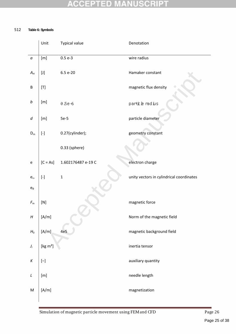
Table 6: Symbols512
Unit Typical value Denotation
a [m] 0.5 e-3 wire radius
AH [J] 6.5 e-20 Hamaker constant
B [T] magnetic flux density
b [m] 0.5e-6 particle radius
d [m] 5e-5 particle diameter
Dm [-] 0.27(cylinder);
0.33 (sphere)
geometry constant
e [C = As] 1.602176487 e-19 C electron charge
er,
eθ
[-] 1 unity vectors in cylindrical coordinates
Fm [N] magnetic force
H [A/m] Norm of the magnetic field
H0 [A/m] 4e5 magnetic background field
Ji [kg m²] inertia tensor
K [–] auxiliary quantity
L [m] needle length
M [A/m] magnetization
Page 26 of 38
Accep
ted
Man
uscr
ipt
Simulation of magnetic particle movement using FEM and CFD Page 27
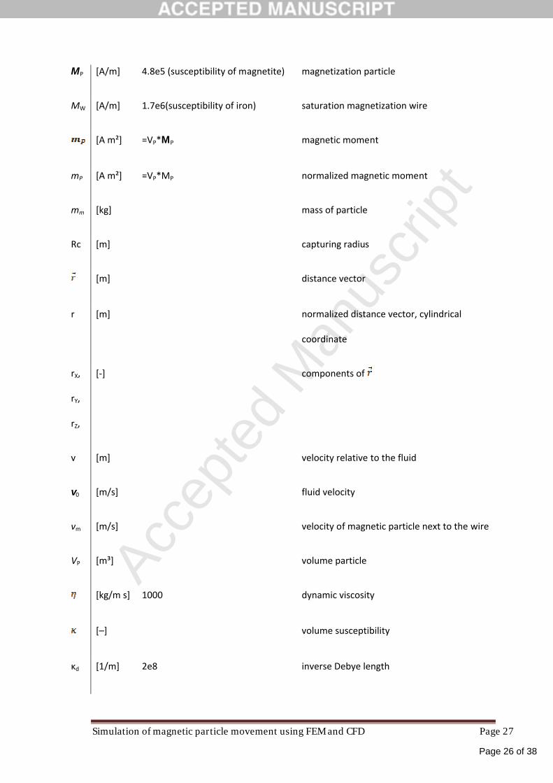
MP [A/m] 4.8e5 (susceptibility of magnetite) magnetization particle
MW [A/m] 1.7e6(susceptibility of iron) saturation magnetization wire
[A m²] =VP*MP magnetic moment
mP [A m²] =VP*MP normalized magnetic moment
mm [kg] mass of particle
Rc [m] capturing radius
[m] distance vector
r [m] normalized distance vector, cylindrical
coordinate
rX,
rY,
rZ,
[-] components of
v [m] velocity relative to the fluid
v0 [m/s] fluid velocity
vm [m/s] velocity of magnetic particle next to the wire
VP [m³] volume particle
[kg/m s] 1000 dynamic viscosity
[–] volume susceptibility
κd [1/m] 2e8 inverse Debye length
Page 27 of 38
Accep
ted
Man
uscr
ipt
Simulation of magnetic particle movement using FEM and CFD Page 28
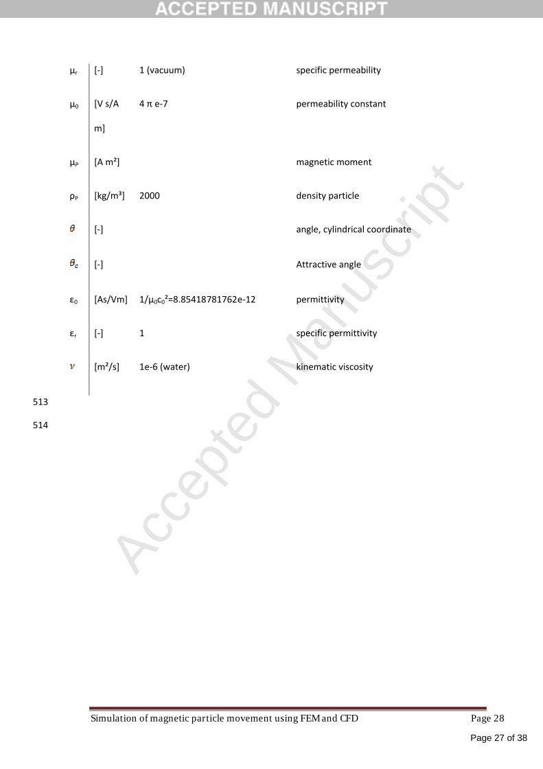
µr [-] 1 (vacuum) specific permeability
µ0 [V s/A
m]
4 π e-7 permeability constant
µP [A m²] magnetic moment
ρP [kg/m³] 2000 density particle
[-] angle, cylindrical coordinate
[-] Attractive angle
ε0 [As/Vm] 1/µ0c0²=8.85418781762e-12 permittivity
εr [-] 1 specific permittivity
[m²/s] 1e-6 (water) kinematic viscosity
513
514
Page 28 of 38
Accep
ted
Man
uscr
ipt
Figure 1
Page 29 of 38
Accep
ted
Man
uscr
ipt
Figure 2
Page 30 of 38
Accep
ted
Man
uscr
ipt
Figure 3
Page 31 of 38
Accep
ted
Man
uscr
ipt
Figure 4
Page 32 of 38
Accep
ted
Man
uscr
ipt
Figure 5
Page 33 of 38
Accep
ted
Man
uscr
ipt
Figure 6
Page 34 of 38
Accep
ted
Man
uscr
ipt
Figure 7
Page 35 of 38
Accep
ted
Man
uscr
ipt
Figure 8
Page 36 of 38
Accep
ted
Man
uscr
ipt
Figure 9

Page 37 of 38
Accep
ted
Man
uscr
ipt
Figure10
Page 38 of 38
Accep
ted
Man
uscr
ipt
Figure11