Simulation of Oil Tank Fires

5/7/2018 Simulation of Oil Tank Fires - slidepdf.com

http://slidepdf.com/reader/full/simulation-of-oil-tank-fires 1/12



atmosphere. Moreover, the phenomena are inherently time dependent and involve a wide temperature

range. Thus, the simplifications employed in ALOFT and its generalizations can not be used in the

present analysis.

The next section presents a hydrodynamic model that contains the components needed to address this

problem. The model consists of a version of the authors three dimensional enclosure fire model3 4 5,

modified to account for a stratified atmosphere. The change is required because the classical “low Mach

number” combustion equations used for enclosure fires assume that the pressure is a small perturbation

about a spatially uniform state that can vary with time as heat from the fire is added to the system 7. In

the present scenario, the fire-induced pressure is a perturbation about a vertically stratified pressure in

approximate hydrostatic balance with prescribed ambient wind and temperature fields. Topographical

features and the built environment are accounted for by blocking portions of the computational domain

to ensure no flux through solid boundaries.

This is supplemented by a radiative transport model described in the third section. The radiation is

emitted as a prescribed fraction of the chemical energy released in each Lagrangian element used to

describe the fire energy input. This fraction, typically in the thirty to thirty five percent range, is the

same as that used previously in the present authors earlier studies of enclosure fires. The difference isthat a fraction of the fuel mass in each burning element is converted to soot. The soot thus introduced is

allowed to absorb radiant energy. The radiant energy flux arriving on the target surface is calculated by

summing the exact solution to the radiative transport equation for a discrete set of point emitters with

a prescribed energy release. The effect of the absorption on the plume hydrodynamics is accounted for

by using the analytical solution to calculate the divergence of the flux from the same random sample of

Lagrangian elements used to compute the surface heat transfer. A check for self-consistency is made by

noting that the fraction of the combustion energy released arriving as radiation on the target surfaces is

close to that estimated from crude oil experiments8.

The approach described above preserves the the efficiency and accuracy of the authors earlier smoke

plume calculations4 5

, and ensures that the radiative transport is calculated from an accurate estimate of the energy emitted rather than from the bulk temperature field. This distinction is important for three

reasons. First, the radiant energy is actually emitted as a result of the same sub-grid scale processes that

govern the combustion energy release. These processes are no more accessible to computation at the

grid resolution than the combustion phenomena simulated by the Lagrangian elements. Second, even

if the bulk temperatures were representative of those in the individual flames where the energy release

actually takes place, there is no reason to believe they could be calculated with sufficient accuracy to

prevent serious errors in the radiative transport computation. Finally, the assumption that all radiation is

emitted from a discrete set of point sources permits an exact solution to the radiative transport equation

to be employed, eliminating the need for detailed computations to solve this equation. The result is a

fully coupled solution to both the fluid dynamics and radiative transport equations that retains both high

resolution and reasonable computer costs.

In the fourth section, the model is applied to a study of the radiative flux induced by fires burning the

contents of an oil storage tank in a 3x3 array. Each tank sits partially depressed in a spill containment

trench surrounded by a sloping embankment. Two possible fire scenarios are considered. The first is a

fire on the top of the tank, maximizing the wind effect on the flame shape. The second is a fire in the

containment trench, which maximizes the role of the tank configuration. For each scenario, two wind

speeds are considered. The wind speed profile and thermal stratification of the atmosphere are selected

to be representative of the atmospheric boundary layer under stable conditions prevalent in northern

winter climates.



OUTDOOR FIRE MODEL

The starting point is the equations of motion for a compressible flow in the low Mach number

approximation. However, the equations as developed by Rehm and Baum7 must be modified to allow for

an ambient pressure P0

¡

z¢, temperature T 0

¡

z¢

and density ρ0

¡

z¢

that vary with height z in the atmosphere

in the absence of the fire. Their equations assume that the fire induced pressure is a small perturbation

about the time dependent spatial average of the pressure in an enclosure. For the present application,

the fire induced pressure ˜ p is a small perturbation about P0

¡

z¢. The ambient density and temperature

are related to P0

¡

z¢ by the equation of state and the assumption of hydrostatic balance in the ambient

atmosphere. The equations expressing the conservation of mass, momentum, and energy then take the

form: Dρ

Dt

£

ρ∇¤¦ ¥u

§ 0 (1)

ρ

¨

∂¥

u

∂t ©

¥

u

¥ω£

∇

¨

1

2u2

£

∇ ˜ p©

¡

ρ©

ρ0 ¢ ¥

g§∇

¤τ (2)

ρC p DT

Dt ©

wdP0

dz§

©

∇¤ ¥q

£

q̇c (3)

Here, ρ is the density,¥u the velocity, T the temperature, and ˜ p the fire induced pressure in the gas.

The unresolved momentum flux and viscous stress tensors are lumped together and denoted by τ. The

quantity ¥ω is the fluid vorticity. The vertical component of the velocity is denoted by w in equation

(3) and the hydrostatic relation between P0 and ρ0 has been used in equation (2). The specific heat is

denoted by C p. Similarly, the unresolved advected energy flux, the conduction heat flux, and the radiant

energy flux are denoted by¥q, while the convective heat release per unit volume is q̇c. These equations

are supplemented by models for τ ¥q, and an equation of state:

P0

¡

z¢ §

ρ

T (4)

The energy and momentum equations can be thought of as advancing the time evolution of the tem-

perature and velocity respectively. However the pressure perturbation does not obey an explicit time

evolution equation. Instead, it is the solution of an elliptic equation determined by the divergence of the

velocity field. This quantity in turn is determined by the mass and energy conservation equations.

The equations presented above also require models for τ and ¥q, as well as a representation of the heat

release from the fire. Two approaches to the unresolved stresses have been used. The bulk of the

large eddy simulations performed to date use a constant eddy viscosity6. This is sufficiently accurate

provided that two conditions are met: First, the grid employed must be fine enough to capture the mixing

at the scales where the eddy viscosity is effective. Second, these scales must be much smaller than

the characteristic plume scale D §

¡

Q!

ρ0C pT 0 " g¢

2 # 5

(see Ref. 5). Alternatively, the second of theseconditions can sometimes be relaxed if a more elaborate sub-grid scale model is used. The calculations

reported below use the Smagorinsky model9 where the sub-grid scale Reynolds stress tensor takes the

form:

τi j § 2ρ¡

C s$

¢

2 %

S%

Si j ; Si j §

1

2

¨

∂ui

∂ x j

£

∂u j

∂ xi

;%

S%

§' & 2 Si j Si j (5)

The constant C s §0

(14, and the grid length scale

$

§

¡

δ xδ yδ z¢

1#

3. In fact, the resolution employed in

the calculations is sufficiently high (a 128x128x128 grid is used with each tank top inscribed within a

14x14 array of cells) for either model to give essentially the same results. The unresolved convective

heat flux is described in terms of an eddy conductivity which is related to the eddy viscosity by a constant

Prandtl number of 0.7.



Finally, the chemical heat release from the fire is represented by a large number N p of Lagrangian

thermal elements whose mathematical representation takes the form6

q̇c §

N p

∑i

)1

¡

1©

χr ¢q̇i

¡

t ¢ δ

¡

¥r

©

¥r i ¢ (6)

Here, δ denotes the Dirac delta function,¥

r i is the location of the ith element, q̇i the net rate at whichchemical energy is deposited by that element in the gas, and χr is the fraction of the chemical energy

converted into thermal radiation. The divergence of the radiative heat flux vector ¥q R, which couples the

radiative and convective transport, is calculated from the point source solution to the radiative transport

equation. This point is discussed in greater detail below.

RADIATION TRANSPORT

A number of approximate techniques are used for the treatment of radiative transport in other present

day CFD based fire simulations. These include, the six flux model10 for two-dimensional and the dis-

crete transfer method11 for three-dimensional (but assumed centerline symmetry) simulations of grey

gas enclosure fires. For their two-dimensional flame spread simulations Yan and Homstedt12 approx-

imate the spectral dependence by combining a narrow-band model with the discrete transfer method.

Another method, used by Bressloff et al.13 in their axisymmetric simulation of a turbulent jet diffusion

flame, is to incorporate a weighted sum of grey gases solution into the discrete transfer method. The dif-

ferent discrete transfer approaches vary mostly according to the degree to which the spectral dependence

of the radiation is included.

Computational cost limits the complexity of the radiation model that can be employed in most fire

simulations. The model presented here is motivated by the same considerations. The simulations using

discrete transfer methods cited above have mostly involved CFD computations with grids of O¡

103¢

©

O¡

104¢

cells. When grids of the size used in the present computations are used, discrete transfer methods

are less attractive. If k rays are launched from each of N 2 boundary points in a three dimensionalsimulation, k must remain fixed as N increases. This condition is needed to ensure enough rays traverse

a given cell in the interior of the computational domain to accurately estimate the net radiant energy

absorbed by the gas in that cell. Moreover, the number of times the computation must be performed

increases linearly with N , as does the complexity of the calculation of each ray. Since this task becomes

prohibitively expensive for computations involving O¡

106¢ cells, additional approximations (employed

even in some of the simulations cited above) must be made. These typically involve either reducing the

number of rays launched from a boundary cell or not updating the radiation calculation on every time

step. The result is that the coupling of the radiation to the convective transport is approximated less

accurately than either of the separate calculations of the transport processes.

The present radiative transport model adapts the idea of a set of discrete emitters to the large eddy simu-lation techniques developed earlier. The analysis is based on the assumption that a prescribed fraction of

the heat released from each thermal element used to describe the fire is radiated away. This emitted flux

χr q̇i is assumed to be the actual radiant energy flux emitted locally by the thermal element. Typically,

this is about thirty-five percent of the energy liberated by combustion processes. More importantly,

this fraction can be estimated from small scale burns of a given fuel, where the absorption by smoke

particulate matter can be neglected.

For a given point ¥r s on the target surface, the radiative flux q R is given by:

q R §

N p

∑i

)

1

χr q̇i

¡

¥r s

©

¥r i ¢0 ¤ ¥

n

4π %

¥r s

©

¥r i

%3

exp¡

©

λ¡

¥

r s 1 ¥

r i ¢ ¢(7)



λ§3 2 5 4 6

r s 7

6

r i

4

0κ

¨

¥r i

£

s

¡

¥r s

©

¥r i ¢

%

¥r s

©

¥r i

%

ds (8)

Here, ¥n is a unit normal to the surface at the point ¥

r s, and N p is the total number of radiating elements at

the instant in question. The divergence of the radiant heat flux to a general point¥

r from the same set of

point emitters is given by:

∇¤¦ ¥q R §

©

κ ¡

¥r

¢

N p

∑i ) 1

χr q̇i

1

4π %

¥r

©

¥r i

%2

exp¡

©

λ¡

¥r

1 ¥r i ¢ ¢

(9)

The absorption coefficient κ ¡

¥r

¢ is taken to be the Planck mean absorption coefficient for soot as calcu-

lated by Atreya and Agrawal14.

κ §

11(86 f v T

§11

(86 Y s

ρT

ρs

¡

cm 7

1¢

(10)

The soot volume fraction f v or mass fraction Y s is calculated by assuming a fixed fraction of the fuel

burned in each Lagrangian thermal element is converted to soot. Thus, at any instant of time, theamount of soot particulate associated with each element is known. Each time the radiation heat transfer

is calculated, this information is smoothed into the grid and κ evaluated for each cell. Since the product

ρT depends only on the ambient pressure, and the soot particulate density ρs is fixed, κ only varies with

the local soot mass fraction.

Note that equations (7), (9), and (8) constitute an exact solution for the radiant heat flux and its diver-

gence in the sense that the angular integrations have been carried out without approximation. Hence,

there is no “ray effect”. The computational task reduces to evaluating the sum over thermal elements

for each target point. The sums are calculated as a running average over several time steps. At each

step, a random sample of O¡

102¢ elements is chosen, and the sum is carried out and suitably weighted

to account for all the emitted radiation. The divergence is calculated at the center of each 2x2x2 block of cells in the computational domain that contains soot. The number of elements sampled per time step

and the number of time steps in the average were chosen so that the product would yield at least 1000

terms in the contribution to each target point on the surface or in the smoke plume. The averaging time

must be shorter than either the plume pulsation time or the surface thermal response time to ensure that

the resolvable large scale fluctuations are incorporated in the computations.

RESULTS AND DISCUSSION

The mathematical model described above was used to study the radiation heat flux from a fire either

on top of or surrounding an oil storage tank. The figures on the following pages display the results of

four simulations performed for this study. A numerical grid consisting of 128 by 128 by 128 cells was

used to span a cubic domain 768 m on a side. The cell size was 6 m by 6 m in the horizontal directions

and ranged from 3 m near the ground to 12 m at the top of the cube in the vertical. The diameter of each

tank was 84 m, the height 27 m. These tanks were incorporated into the calculation by “blocking” cells.

Because boundary layers are not resolvable (except the planetary boundary layer) at this grid resolution,

there is little penalty in assuming that the tank walls are not smooth, but rather are saw-toothed. Each

tank was depressed below ground level and surrounded by an embankment of height 9 m. The geometry

of each tank and its associated “trench” were modeled on the oil storage facility of the Japan National

Oil Corporation at Tomakomai. No attempt was made to simulate the entire facility, which contains over

80 tanks.



FIGURE 1: Instantaneous snapshot of a tank fire simulation with the wind speed 6 m/s at the tops

of the tanks and the fire in the trench.

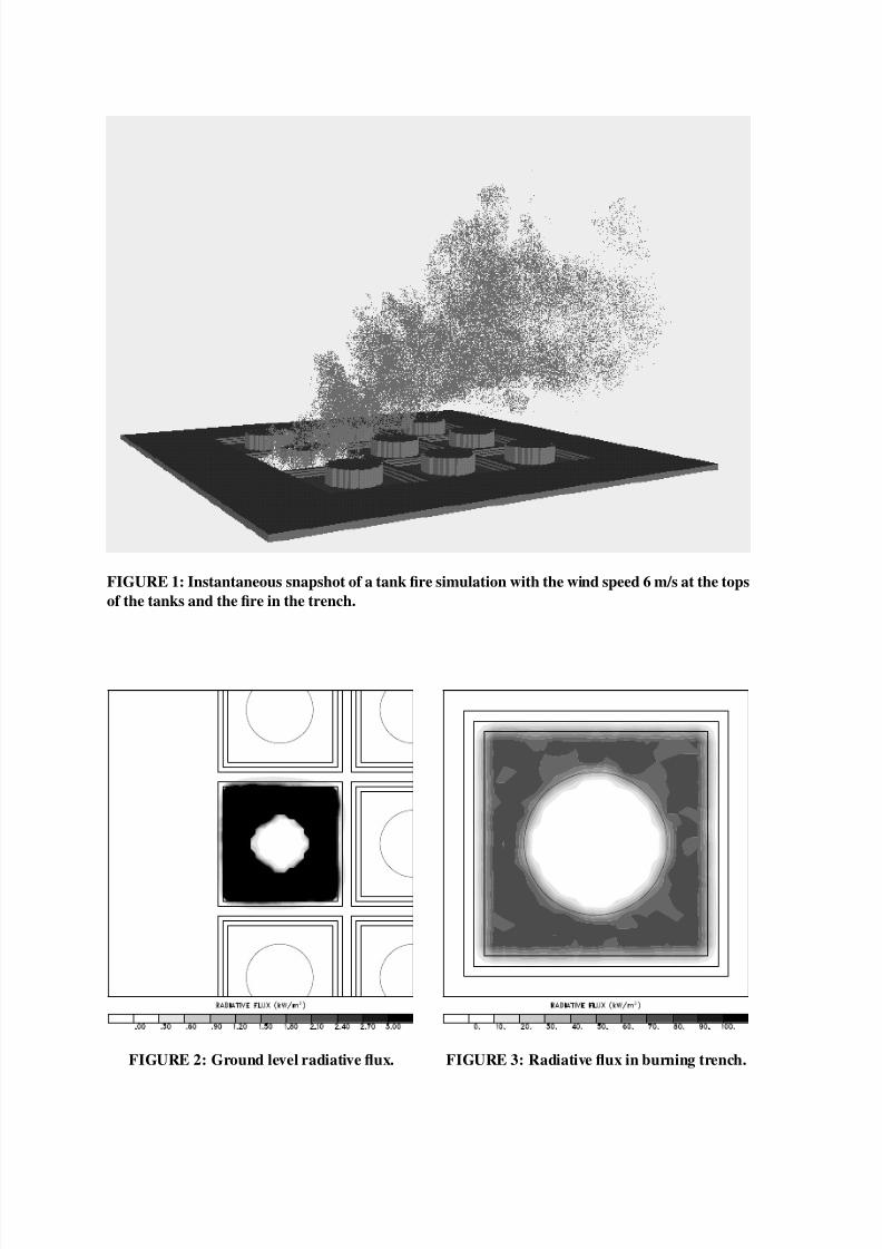
FIGURE 2: Ground level radiative flux. FIGURE 3: Radiative flux in burning trench.



FIGURE 4: Instantaneous snapshot of a tank fire simulation with the wind speed 6 m/s at the tops

of the tanks and the fire on the tank.

FIGURE 5: Ground level radiative flux. FIGURE 6: Radiative flux on the tank top.



FIGURE 7: Instantaneous snapshot of a tank fire simulation with the wind speed 12 m/s at the

tops of the tanks and the fire in the trench.

FIGURE 8: Ground level radiative flux. FIGURE 9: Radiative flux in burning trench.



FIGURE 10: Instantaneous snapshot of a tank fire simulation with the wind speed 12 m/s at the

tops of the tanks and the fire on the tank.

FIGURE 11: Ground level radiative flux. FIGURE 12: Radiative flux on tank top.



A stratified wind profile of the form

u¡

z¢8 §

u0

¨

z

z0

p

(11)

was imposed as a boundary condition. The wind speed u0 at the height of the tanks ( z0 § 27 m) was

6 m/s for two of the simulations and 12 m/s for the other two. The exponent p, a function of the surface

roughness, was 0.15. The temperature of the ambient atmosphere was assumed to be uniform withheight (20

9C), although any resolvable temperature profile can be input. The fire was either assumed to

be engulfing the entire top of the tank, burning with a heat release rate of 1,000 kW/m2, for a total of

5.3 GW; or burning spilled oil in the trench for a total of 12.1 GW. The fraction of the chemical heat

release rate converted into thermal radiation and emitted from the thermal elements was assumed to be

35%.

Figures 1, 4, 7, and 10 show instantaneous snapshots of the Lagrangian elements that represent the fire

plume in the simulations. The bright colored elements are burning; releasing energy into the gas and

the radiation field. Thus, the composite burning elements represent the instantaneous flame structure

at the resolution limit of the simulation. The dark colored elements are burnt out. They represent the

smoke and gaseous combustion products that absorb the radiant energy from the flames. It is important

to understand how much of the emitted radiant energy is re-absorbed by the surrounding smoke. The

magnitude of this smoke shielding can be realized by computing the radiative flux to the surrounding

tanks. For the case of the burning tank top in a 6 m/s wind (Fig. 1), the radiative flux to the side of the

downwind tank was 1.6 kW/m2. A test calculation was performed in which no thermal radiation was

absorbed by the smoke. For this case, the flux to the downwind tank was 9.0 kW/m 2. Thus the effective

radiative fraction is¡

1 ( 6 ! 9 ( 0 ¢ 35% or about 6%. This estimate is consistent with the measurements of

Koseki8. Note that the actual measurements were made from a single point using a detector that “saw”

the entire plume. Thus, it is essentially the same quantity as that calculated in the present paper. The

interpretation of this result as a global estimate of the radiative fraction involves additional assumptions

that will not be made here. To explore this point further, a separate simulation of a vertical plume in the

absence of any wind was performed. The convective energy flux at several heights above the fire bed

was calculated. The energy flux was consistently approximately 94% of the total heat release rate in thefire. This means that of the original 35% released as thermal radiation, 29% was reabsorbed.

The combined effects of wind and geometry are apparent in the figures below. The intense radiation is

largely confined to the containment trenches for those fires originating in the trench regardless of wind

speed. Comparison of Fig. 3 with Fig. 9 shows that the radiation levels in the trench are higher and more

uniformly distributed for the 6 m/s wind than for the higher wind speed. At the higher speed, the flames

and smoke are shifted somewhat more downwind. As a result, the upwind surface is more exposed to

the flame radiation, and the downwind surface more shielded by the smoke, skewing the surface flux

contours. Figures 5 and 11 show that the tank top fires generate downwind and lateral ground level

fluxes, although the most intense radiation is back to the burning surface. The fluxes in the firebed for

the tank top fires are shown in Figures 6 and 12. The peak values are about 10 kW/m2 higher for thetank top fires than for the trench fires. Moreover, the higher wind exposes more of the upwind tank top

surface to unshielded flames and blocking more of the radiation on the downwind portion of the surface

than in the lower wind case.

The calculations simulated 180 seconds of real time with an average time step of 0.09 seconds. This

required from approximately 29 to 48 hours of CPU time per simulation, depending on the number of

radiating elements chosen per time step. The radiative transport calculation was tested by selecting from

50 to 200 elements per time step and using a 5 to 20 time step running average. The radiation transport

consumed about 20% to 50% of the total CPU time. The 5 time step averaging period corresponded

to less than 10% of the pulsation period of the fire plume. The results for the radiative transport were



insensitive to the choice of averaging time within this parameter range. All calculations were performed

on an IBM RS6000 model 595 server. Approximately 600 MBytes of memory was used.

The above examples illustrate the complex interaction between the topography, the ambient atmosphere,

and the fire dynamics. Even for the relatively simple configuration chosen for study here, there are many

factors that strongly affect the resulting fire dynamics. The ambient wind and temperature fields must

play at least as significant a role as they do in the downwind smoke dispersion described by the ALOFT

code. The presence of natural topographical features in the vicinity of the storage tanks would further

modify the flow patterns, and hence the radiation fields. Rather than arbitrarily choosing topographical,

structural, and meteorological features to simulate, it would seem to make more sense to couple the

emerging simulation capability to databases that describe the actual built environment and associated

topography. Similarly, arbitrary prescriptions of the ambient atmosphere could be replaced with local

meteorology simulations based on databases and computer models in use by the weather prediction

community. The result would be a simulation capability that could be used routinely to predict the fire

hazards resulting from natural or man made disasters in the real world.

REFERENCES

1. Baum, H.R., McGrattan, K.B., and Rehm, R.G., “Simulation of Smoke Plumes from Large Pool

Fires”, Twenty Fifth Symposium (International) on Combustion, The Combustion Institute, Pitts-

burgh, pp. 1463-1469, (1994).

2. McGrattan, K.B., Baum, H.R., and Rehm, R.G., “Numerical Simulation of Smoke Plumes from

Large Oil Fires”, Atmospheric Environment , Vol. 30, pp. 4125-4136, (1996).

3. McGrattan, K.B., Baum, H.R., Walton, W.D., and Trelles, J., “Smoke Plume Trajectory from In

Situ Burning of Crude Oil in Alaska — Field Experiments and Modeling of Complex Terrain”,

NISTIR 5958, National Institute of Standards and Technology, Gaithersburg, (1997).

4. Baum, H.R., McGrattan, K.B., and Rehm, R.G., “Three Dimensional Simulation of Fire Plume

Dynamics”, Jour. Heat Trans. Soc. Japan, Vol. 35, pp. 45-52, (1996).

5. Baum, H.R., McGrattan, K.B., and Rehm, R.G., “Three Dimensional Simulation of Fire Plume

Dynamics”, Fire Safety Science - Proceedings of the Fifth International Symposium, Y. Hasemi,

Ed., International Association for Fire Safety Science, pp. 511-522, (1997).

6. McGrattan, K.B., Baum, H.R., and Rehm, R.G., “Large Eddy Simulations of Smoke Movement”,

Fire Safety Journal, Vol. 30, pp. 161-178, (1998).

7. Rehm, R.G. and Baum, H.R., “The Equations of Motion for Thermally Driven, Buoyant Flows”,

J. Research of Nat. Bur. Standards, Vol. 83, pp. 297-308, (1978).

8. Koseki, H. and Mulholland, G.W., “The effect of diameter on the burning of crude oil pool fires,”

Fire Technology, Vol. 54 (1991).

9. Smagorinsky, J., “General Circulation Experiments with the Primitive Equations. I. The Basic

Experiment”, Monthly Weather Review, Vol. 91, pp. 99-164, (1963).

10. Jia, F., Galea, E.R., and Patel, M.K., “The Prediction of Fire Propagation in Enclosure Fires”, Fire

Safety Science - Proceedings of the Fifth International Symposium, Y. Hasemi, Ed., pp. 439-450,

(1997).



11. Lewis, M.J., Moss, M.B., and Rubini, P.A., “CFD Modeling of Combustion and Heat Transfer in

Compartment Fires”, Fire Safety Science - Proceedings of the Fifth International Symposium, Y.

Hasemi, Ed., pp. 463-474, (1997).

12. Yan, Z. and Holmstedt, G., “CFD Simulation of Upward Flame Spread over Fuel Surfaces”, Fire

Safety Science - Proceedings of the Fifth International Symposium, Y. Hasemi, Ed., pp. 345-355,

(1997).

13. Bressloff, N.W., Moss, J.B., and Rubini, P.A., “CFD Prediction of Coupled Radiation Heat Trans-

fer and Soot Production in Turbulent Flames”, Twenty Sixth Symposium (International) on Com-

bustion, The Combustion Institute, Pittsburgh, pp. 2379-2386, (1996).

14. Atreya, A. and Agrawal, A., “Effect of Heat Loss on Diffusion Flames”, Combustion and Flame,

Vol. 115, pp. 372-382, (1998).

Documents

Simulation of Oil Tank Fires