Simulation of Railway Power Supply Systems - …openpowernet.de/downloads/summary/OPN_OT_summary_en.pdf · Simulation of . Railway Power Supply Systems . in Co-Simulation with . Program

Simulation of

Railway Power Supply Systems

in Co-Simulation with

Program Description

and References

2018-03-29

OpenPowerNet users

Dresden,

Germany

Wuhan,

PR China

Brisbane,

Australia

Shanghai,

PR China

Madrid,

Spain

Wollongong,

Australia

Melbourne,

Australia

Chengdu,

PR China

Beijing,

PR China

São Paulo,

Brazil

Mexico City,

Mexico

Macau

Rio de Janeiro,

Brazil

Hongkong

Lyon,

France

Summary Page 2/35

2018-03-29

OpenPowerNet users

Wrocław,

Poland

Perth,

Australia

Medellin,

Colombia

Newark,

USA

Brussels,

Belgium

Brno,

Czech Republic

Meidensha,

Japan

Beijing,

PR China

Ontario,

Canada

Bangalore,

India

Hongkong

Singapore

Bangkok,

Thailand

Bandung,

Indonesia

Summary Page 3/35

OpenPowerNet_2008.doc 1 / 12 14/05/2008

OpenPowerNet – Simulation of Railway Power Supply Systems

Prof. Dr.-Ing. Arnd Stephan, Dipl.-Ing. (FH) Martin Jacob, Dipl.-Ing. (FH) Harald Scheiner IFB Institut für Bahntechnik GmbH, Dresden, Germany Wiener Str. 114-116, 01219 Dresden [email protected], www.bahntechnik.de

Abstract

The energy consumption of electrical railways is mainly influenced by the driving states and the propulsion efficiency characteristics of the trains as well as by the behaviour of the traction power supply system. For this reason the idea was to create a plug-in simulation module for railway power supply networks using the advanta-ges of an existing commercial railway operation simulator. The new developed energy simulation module called OpenPowerNet works together with the Swiss OpenTrack railway operation simulator as a so called “co-simula-tion”. OpenPowerNet is able to simulate all common AC- and DC-railway power supply systems taking into account the entire electrical network structure. It can be used as an energy prognosis and analysis tool as well as for the planning and optimisation of power supply installations. The accuracy of the simulation was verified by a lot of realtime measurements. Keywords: Simulation Tools, Planning, Operations Quality, Energy Management, Power Supply Systems

1 Introduction

For prognosis and analysis of railway energy consumption the use of simulation tools is state of the art today. For that purpose a considerable number of software tools with different preciseness is available. But the modern software technology offers new possibilities to improve the simulation. The electrical load flow within railway power supply networks and the train energy consumption depend both on the running trains and the power supply system characteristics. In contrast to public energy distribution systems there are moving energy consumers with a time-dependent power demand picking up and recovering energy at changing locations. The network structure and the voltage situation influence the internal load flows because: • currents and power losses increase with decreasing voltages, • under low voltage conditions current or power limitations of the train propulsion control can be activated

with impact on the driving dynamics, • the network voltage determines the braking energy recovering decisively.

Thus the power supply system may influence the traction characteristics of the trains and the railway energy consumption. The simulation of these dynamic processes allows the analysis and prognosis of load flows and energy consumption as well as the design and rating verification of the electrical installations. However a realistic prog-nosis by simulation requires detailed information about the present power consumption, the actual position of the trains and the capability of the power supply network available simultaneously. Therefore a series of compromi-ses either concerning the railway operation simulation or the electrical network modelling depth were made in the past. For this reason the idea was to create a plug-in simulation module for railway power supply networks using the advantages of an existing commercial railway operation simulator.

Summary Page 4/35


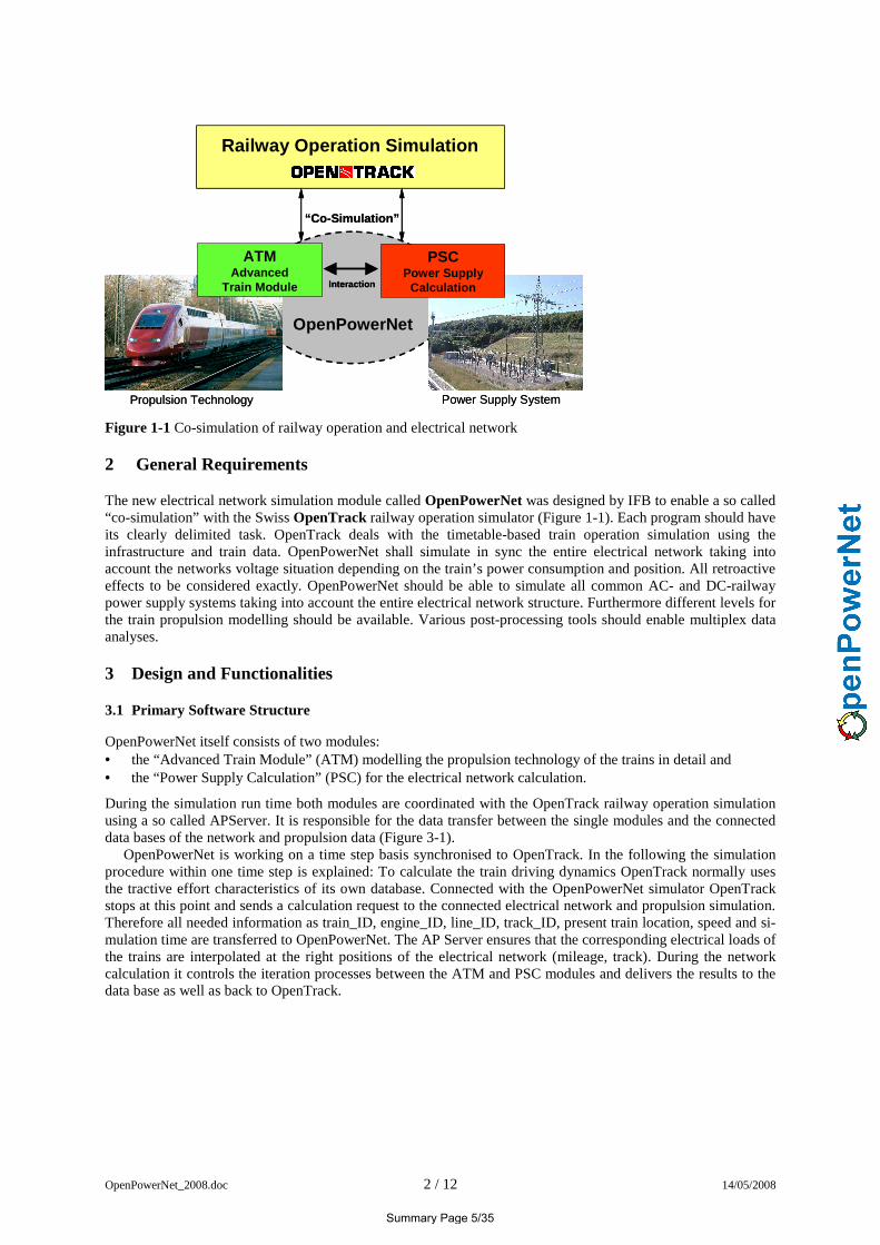
OpenPowerNetOpenPowerNet

Propulsion TechnologyPropulsion Technology

Railway Operation Simulation

ATMAdvanced

Train Module

“Co-Simulation”“Co-Simulation”

Power Supply SystemPower Supply System

PSCPower Supply

CalculationInteractionInteraction

Figure 1-1 Co-simulation of railway operation and electrical network

2 General Requirements

The new electrical network simulation module called OpenPowerNet was designed by IFB to enable a so called “co-simulation” with the Swiss OpenTrack railway operation simulator (Figure 1-1). Each program should have its clearly delimited task. OpenTrack deals with the timetable-based train operation simulation using the infrastructure and train data. OpenPowerNet shall simulate in sync the entire electrical network taking into account the networks voltage situation depending on the train’s power consumption and position. All retroactive effects to be considered exactly. OpenPowerNet should be able to simulate all common AC- and DC-railway power supply systems taking into account the entire electrical network structure. Furthermore different levels for the train propulsion modelling should be available. Various post-processing tools should enable multiplex data analyses.

3 Design and Functionalities

3.1 Primary Software Structure

OpenPowerNet itself consists of two modules: • the “Advanced Train Module” (ATM) modelling the propulsion technology of the trains in detail and • the “Power Supply Calculation” (PSC) for the electrical network calculation.

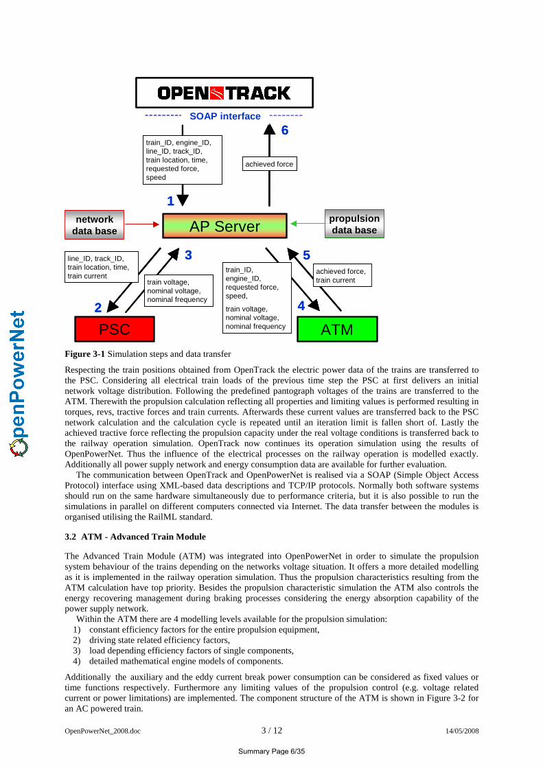
During the simulation run time both modules are coordinated with the OpenTrack railway operation simulation using a so called APServer. It is responsible for the data transfer between the single modules and the connected data bases of the network and propulsion data (Figure 3-1). OpenPowerNet is working on a time step basis synchronised to OpenTrack. In the following the simulation procedure within one time step is explained: To calculate the train driving dynamics OpenTrack normally uses the tractive effort characteristics of its own database. Connected with the OpenPowerNet simulator OpenTrack stops at this point and sends a calculation request to the connected electrical network and propulsion simulation. Therefore all needed information as train_ID, engine_ID, line_ID, track_ID, present train location, speed and si-mulation time are transferred to OpenPowerNet. The AP Server ensures that the corresponding electrical loads of the trains are interpolated at the right positions of the electrical network (mileage, track). During the network calculation it controls the iteration processes between the ATM and PSC modules and delivers the results to the data base as well as back to OpenTrack.

Summary Page 5/35


AP Server

PSC ATM

network data base

propulsion data base

train_ID, engine_ID,line_ID, track_ID,train location, time,requested force,speed

1

train_ID, engine_ID,line_ID, track_ID,train location, time,requested force,speed

1

line_ID, track_ID,train location, time, train current

2

line_ID, track_ID,train location, time, train current

2

train voltage, nominal voltage,nominal frequency

3

train voltage, nominal voltage,nominal frequency

3train_ID,engine_ID, requested force,speed,

train voltage,nominal voltage,nominal frequency

4

train_ID,engine_ID, requested force,speed,

train voltage,nominal voltage,nominal frequency

4

achieved force,train current

5achieved force,train current

5

achieved force

6

achieved force

6SOAP interfaceSOAP interface

Figure 3-1 Simulation steps and data transfer

Respecting the train positions obtained from OpenTrack the electric power data of the trains are transferred to the PSC. Considering all electrical train loads of the previous time step the PSC at first delivers an initial network voltage distribution. Following the predefined pantograph voltages of the trains are transferred to the ATM. Therewith the propulsion calculation reflecting all properties and limiting values is performed resulting in torques, revs, tractive forces and train currents. Afterwards these current values are transferred back to the PSC network calculation and the calculation cycle is repeated until an iteration limit is fallen short of. Lastly the achieved tractive force reflecting the propulsion capacity under the real voltage conditions is transferred back to the railway operation simulation. OpenTrack now continues its operation simulation using the results of OpenPowerNet. Thus the influence of the electrical processes on the railway operation is modelled exactly. Additionally all power supply network and energy consumption data are available for further evaluation. The communication between OpenTrack and OpenPowerNet is realised via a SOAP (Simple Object Access Protocol) interface using XML-based data descriptions and TCP/IP protocols. Normally both software systems should run on the same hardware simultaneously due to performance criteria, but it is also possible to run the simulations in parallel on different computers connected via Internet. The data transfer between the modules is organised utilising the RailML standard.

3.2 ATM - Advanced Train Module

The Advanced Train Module (ATM) was integrated into OpenPowerNet in order to simulate the propulsion system behaviour of the trains depending on the networks voltage situation. It offers a more detailed modelling as it is implemented in the railway operation simulation. Thus the propulsion characteristics resulting from the ATM calculation have top priority. Besides the propulsion characteristic simulation the ATM also controls the energy recovering management during braking processes considering the energy absorption capability of the power supply network. Within the ATM there are 4 modelling levels available for the propulsion simulation:

1) constant efficiency factors for the entire propulsion equipment, 2) driving state related efficiency factors, 3) load depending efficiency factors of single components, 4) detailed mathematical engine models of components.

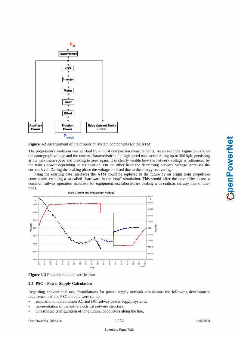
Additionally the auxiliary and the eddy current break power consumption can be considered as fixed values or time functions respectively. Furthermore any limiting values of the propulsion control (e.g. voltage related current or power limitations) are implemented. The component structure of the ATM is shown in Figure 3-2 for an AC powered train.

Summary Page 6/35


Pel

Pmech

Figure 3-2 Arrangement of the propulsion system components for the ATM

The propulsion simulation was verified by a lot of comparison measurements. As an example Figure 3-3 shows the pantograph voltage and the current characteristics of a high speed train accelerating up to 300 kph, persisting at the maximum speed and braking to zero again. It is clearly visible how the network voltage is influenced by the train’s power depending on its position. On the other hand the decreasing network voltage increases the current level. During the braking phase the voltage is raised due to the energy recovering. Using the existing data interfaces the ATM could be replaced in the future by an origin train propulsion control unit enabling a so-called “hardware in the loop” simulation. This would offer the possibility to use a common railway operation simulator for equipment test laboratories dealing with realistic railway line simula-tions.

23000

23500

24000

24500

25000

25500

26000

26500

27000

00:0

0

00:3

0

01:0

0

01:3

0

02:0

0

02:3

0

03:0

0

03:3

0

04:0

0

04:3

0

05:0

0

05:3

0

06:0

0

06:3

0

07:0

0

07:3

0

08:0

0

08:3

0

09:0

0

Zeit in Minuten

Spa

nnun

g in

Vol

t

-500,00

-400,00

-300,00

-200,00

-100,00

0,00

100,00

200,00

300,00

400,00

500,00

Stro

m in

Am

pere

Spannung in Volt Strom in Ampere

time h:min

volta

ge

curr

ent

AV

Train Current and Pantograph Voltage

Figure 3-3 Propulsion model verification

3.3 PSC – Power Supply Calculation

Regarding conventional task formulations for power supply network simulations the following development requirements to the PSC module were set up: • simulation of all common AC and DC railway power supply systems, • representation of the entire electrical network structure, • unrestricted configuration of longitudinal conductors along the line,

Summary Page 7/35


• precise consideration of the electromagnetic coupling effects between the longitudinal conductors within single phase AC systems,

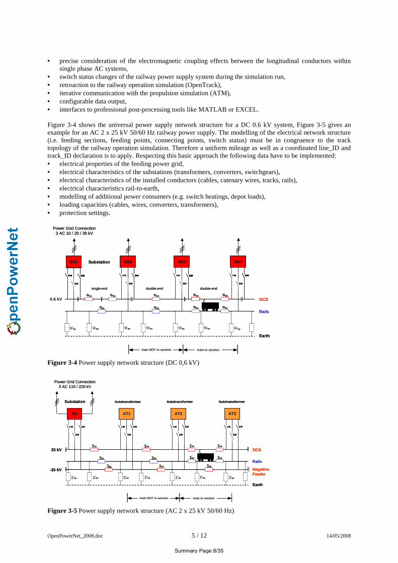
• switch status changes of the railway power supply system during the simulation run, • retroaction to the railway operation simulation (OpenTrack), • iterative communication with the propulsion simulation (ATM), • configurable data output, • interfaces to professional post-processing tools like MATLAB or EXCEL. Figure 3-4 shows the universal power supply network structure for a DC 0.6 kV system, Figure 3-5 gives an example for an AC 2 x 25 kV 50/60 Hz railway power supply. The modelling of the electrical network structure (i.e. feeding sections, feeding points, connecting points, switch status) must be in congruence to the track topology of the railway operation simulation. Therefore a uniform mileage as well as a coordinated line_ID and track_ID declaration is to apply. Respecting this basic approach the following data have to be implemented: • electrical properties of the feeding power grid, • electrical characteristics of the substations (transformers, converters, switchgears), • electrical characteristics of the installed conductors (cables, catenary wires, tracks, rails), • electrical characteristics rail-to-earth, • modelling of additional power consumers (e.g. switch heatings, depot loads), • loading capacities (cables, wires, converters, transformers), • protection settings.

Power Grid Connection3 AC 10 / 20 / 30 kV

OCS

Rails

train NOT in section train in section

Substation

GO1

GR1

GO3

GR2

GO4

GR3

GO5

GR4

sw

sw

SS1

sw

sw

SS2

sw

sw

SS3

sw

sw

SS4

Earth

G’RE G’RE G’RE G’RE G’RE G’RE G’RE

sw sw sw sw

GO2

single-end double-end double-end

Power Grid Connection3 AC 10 / 20 / 30 kV

OCS

Rails

train NOT in section train in sectiontrain NOT in section train in section

Substation

GO1

GR1

GO3

GR2

GO4

GR3

GO5

GR4

swsw

sw

SS1

sw

sw

SS2

sw

sw

SS3

sw

sw

SS4

Earth

G’RE G’RE G’RE G’RE G’RE G’RE G’RE

swsw swsw swsw swsw

GO2

single-end double-end double-end

0.6 kV

Figure 3-4 Power supply network structure (DC 0,6 kV)

OCS

Rails

Negative Feeder

train NOT in section train in section

AutotransformerSubstation

YO1

YR1

YN1

Autotransformer Autotransformer

YO2

YR2

YN2

YO3

YR3

YN3

YO4

YR4

sw

sw

sw

SS

sw

sw

sw

AT1

sw

sw

sw

AT2

sw

sw

sw

AT3

Power Grid Connection3 AC 110 / 220 kV

Earth

Y’RE Y’RE Y’RE Y’RE Y’RE Y’RE Y’RE

25 kV

-25 kV

OCS

Rails

Negative Feeder

train NOT in section train in sectiontrain NOT in section train in section

AutotransformerSubstation

YO1

YR1

YN1

Autotransformer Autotransformer

YO2

YR2

YN2

YO3

YR3

YN3

YO4

YR4

sw

sw

sw

SS

sw

sw

sw

AT1

sw

sw

sw

AT2

sw

sw

sw

AT3

Power Grid Connection3 AC 110 / 220 kV

Earth

Y’RE Y’RE Y’RE Y’RE Y’RE Y’RE Y’RE

25 kV

-25 kV

Figure 3-5 Power supply network structure (AC 2 x 25 kV 50/60 Hz)

Summary Page 8/35


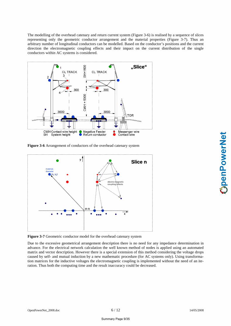
The modelling of the overhead catenary and return current system (Figure 3-6) is realised by a sequence of slices representing only the geometric conductor arrangement and the material properties (Figure 3-7). Thus an arbitrary number of longitudinal conductors can be modelled. Based on the conductor’s positions and the current direction the electromagnetic coupling effects and their impact on the current distribution of the single conductors within AC systems is considered.

„Slice“„Slice“

Figure 3-6 Arrangement of conductors of the overhead catenary system

y

x

y

x

(0; 0)(0; 0)

(x1; y1)(x1; y1)

material, diameter

electro-magneticcoupling effectselectro-magneticcoupling effects

Slice nSlice n

Figure 3-7 Geometric conductor model for the overhead catenary system

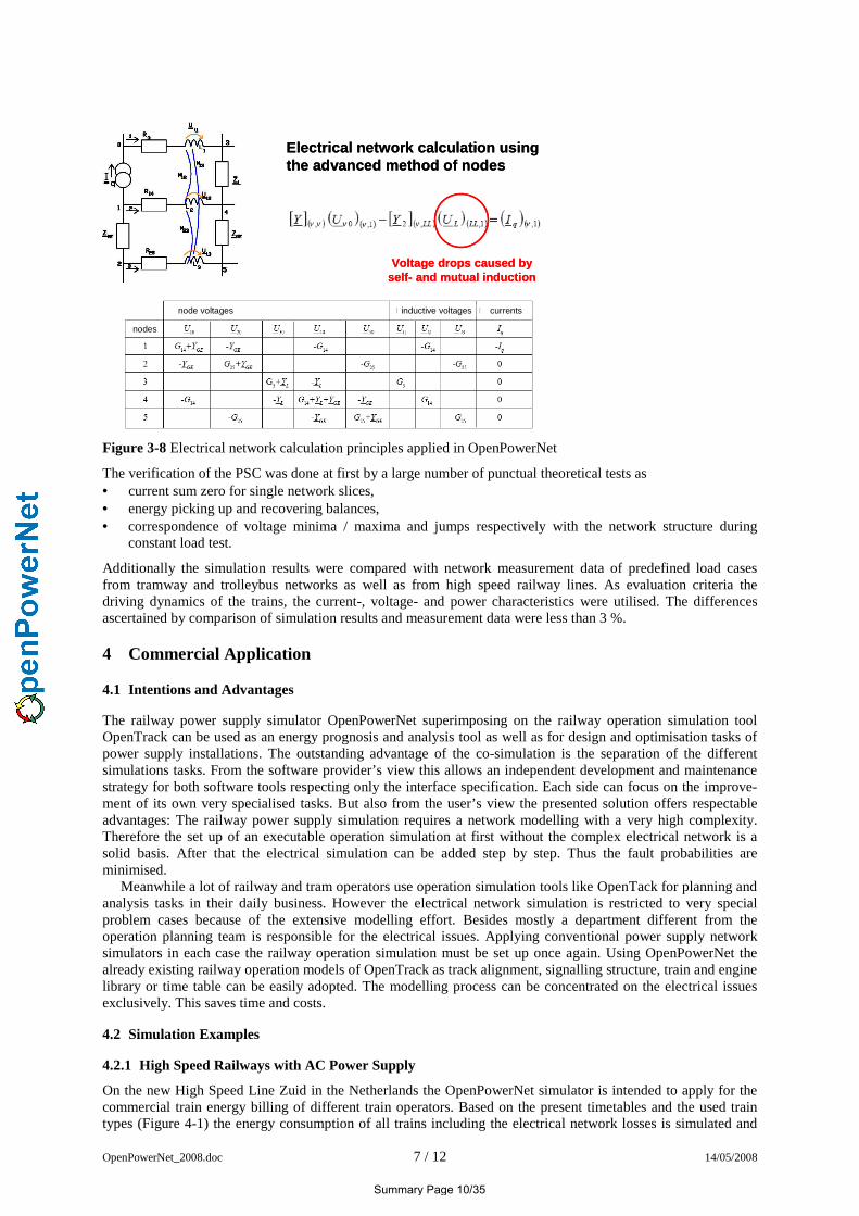
Due to the excessive geometrical arrangement description there is no need for any impedance determination in advance. For the electrical network calculation the well known method of nodes is applied using an automated matrix and vector description. However there is a special extension of this method considering the voltage drops caused by self- and mutual induction by a new mathematic procedure (for AC systems only). Using transforma-tion matrices for the inductive voltages the electromagnetic coupling is implemented without the need of an ite-ration. Thus both the computing time and the result inaccuracy could be decreased.

Summary Page 9/35


Electrical network calculation using the advanced method of nodesElectrical network calculation using the advanced method of nodes

Voltage drops caused by self- and mutual inductionVoltage drops caused by

self- and mutual induction

nodes

node voltages inductive voltages currents

Figure 3-8 Electrical network calculation principles applied in OpenPowerNet

The verification of the PSC was done at first by a large number of punctual theoretical tests as • current sum zero for single network slices, • energy picking up and recovering balances, • correspondence of voltage minima / maxima and jumps respectively with the network structure during

constant load test.

Additionally the simulation results were compared with network measurement data of predefined load cases from tramway and trolleybus networks as well as from high speed railway lines. As evaluation criteria the driving dynamics of the trains, the current-, voltage- and power characteristics were utilised. The differences ascertained by comparison of simulation results and measurement data were less than 3 %.

4 Commercial Application

4.1 Intentions and Advantages

The railway power supply simulator OpenPowerNet superimposing on the railway operation simulation tool OpenTrack can be used as an energy prognosis and analysis tool as well as for design and optimisation tasks of power supply installations. The outstanding advantage of the co-simulation is the separation of the different simulations tasks. From the software provider’s view this allows an independent development and maintenance strategy for both software tools respecting only the interface specification. Each side can focus on the improve-ment of its own very specialised tasks. But also from the user’s view the presented solution offers respectable advantages: The railway power supply simulation requires a network modelling with a very high complexity. Therefore the set up of an executable operation simulation at first without the complex electrical network is a solid basis. After that the electrical simulation can be added step by step. Thus the fault probabilities are minimised. Meanwhile a lot of railway and tram operators use operation simulation tools like OpenTack for planning and analysis tasks in their daily business. However the electrical network simulation is restricted to very special problem cases because of the extensive modelling effort. Besides mostly a department different from the operation planning team is responsible for the electrical issues. Applying conventional power supply network simulators in each case the railway operation simulation must be set up once again. Using OpenPowerNet the already existing railway operation models of OpenTrack as track alignment, signalling structure, train and engine library or time table can be easily adopted. The modelling process can be concentrated on the electrical issues exclusively. This saves time and costs.

4.2 Simulation Examples

4.2.1 High Speed Railways with AC Power Supply

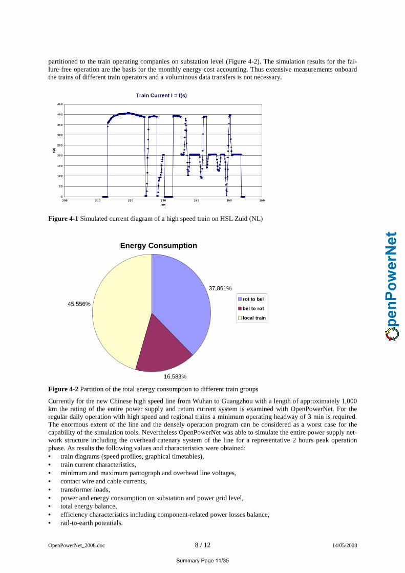
On the new High Speed Line Zuid in the Netherlands the OpenPowerNet simulator is intended to apply for the commercial train energy billing of different train operators. Based on the present timetables and the used train types (Figure 4-1) the energy consumption of all trains including the electrical network losses is simulated and

Summary Page 10/35


partitioned to the train operating companies on substation level (Figure 4-2). The simulation results for the fai-lure-free operation are the basis for the monthly energy cost accounting. Thus extensive measurements onboard the trains of different train operators and a voluminous data transfers is not necessary.

Train C urren t

0

50

100

150

200

250

300

350

400

450

200 2 10 220 230 240 250 260

km

I [A

]

Train Current I = f(s)Train C urren t

0

50

100

150

200

250

300

350

400

450

200 2 10 220 230 240 250 260

km

I [A

]

Train Current I = f(s)

Figure 4-1 Simulated current diagram of a high speed train on HSL Zuid (NL)

Energy Consumption

37,861%

16,583%

45,556%rot to bel

bel to rot

local train

Figure 4-2 Partition of the total energy consumption to different train groups

Currently for the new Chinese high speed line from Wuhan to Guangzhou with a length of approximately 1,000 km the rating of the entire power supply and return current system is examined with OpenPowerNet. For the regular daily operation with high speed and regional trains a minimum operating headway of 3 min is required. The enormous extent of the line and the densely operation program can be considered as a worst case for the capability of the simulation tools. Nevertheless OpenPowerNet was able to simulate the entire power supply net-work structure including the overhead catenary system of the line for a representative 2 hours peak operation phase. As results the following values and characteristics were obtained: • train diagrams (speed profiles, graphical timetables), • train current characteristics, • minimum and maximum pantograph and overhead line voltages, • contact wire and cable currents, • transformer loads, • power and energy consumption on substation and power grid level, • total energy balance, • efficiency characteristics including component-related power losses balance, • rail-to-earth potentials.

Summary Page 11/35


4.2.2 Tramway and Trolley Bus Networks with DC Power Supply

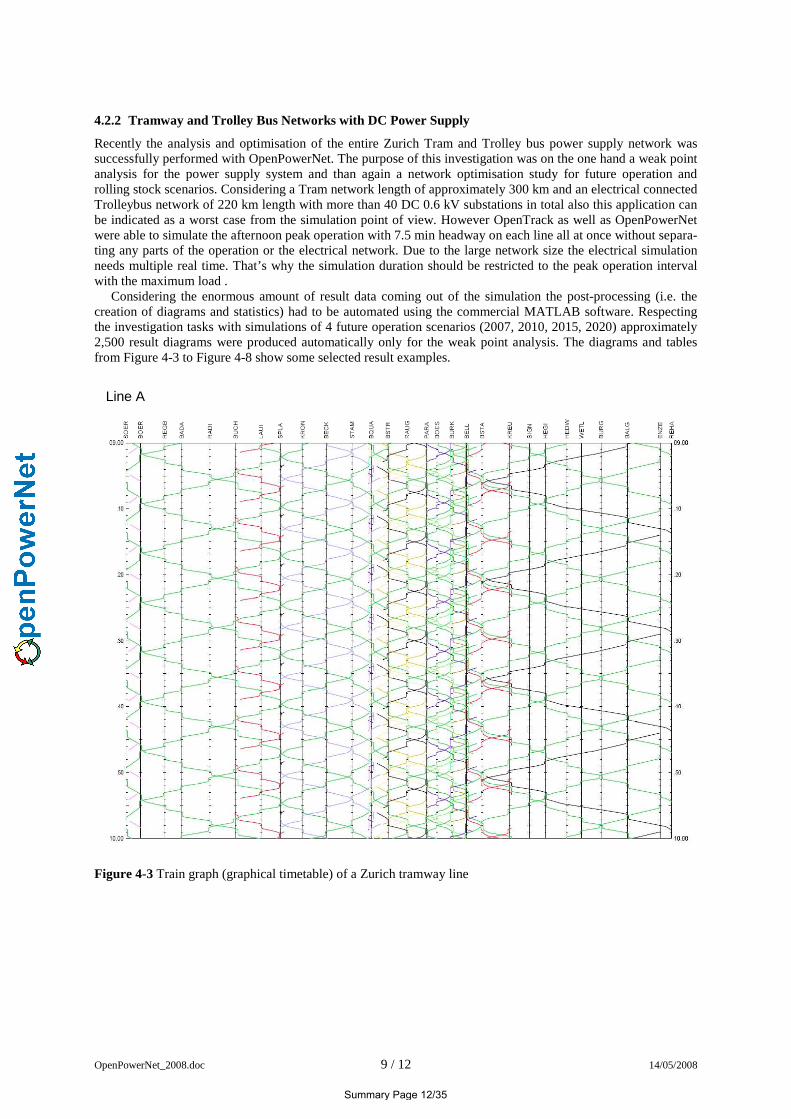
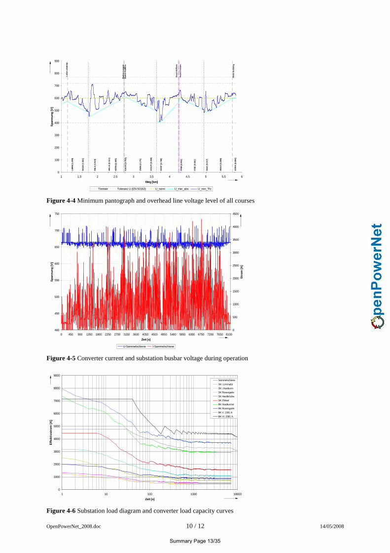
Recently the analysis and optimisation of the entire Zurich Tram and Trolley bus power supply network was successfully performed with OpenPowerNet. The purpose of this investigation was on the one hand a weak point analysis for the power supply system and than again a network optimisation study for future operation and rolling stock scenarios. Considering a Tram network length of approximately 300 km and an electrical connected Trolleybus network of 220 km length with more than 40 DC 0.6 kV substations in total also this application can be indicated as a worst case from the simulation point of view. However OpenTrack as well as OpenPowerNet were able to simulate the afternoon peak operation with 7.5 min headway on each line all at once without separa-ting any parts of the operation or the electrical network. Due to the large network size the electrical simulation needs multiple real time. That’s why the simulation duration should be restricted to the peak operation interval with the maximum load . Considering the enormous amount of result data coming out of the simulation the post-processing (i.e. the creation of diagrams and statistics) had to be automated using the commercial MATLAB software. Respecting the investigation tasks with simulations of 4 future operation scenarios (2007, 2010, 2015, 2020) approximately 2,500 result diagrams were produced automatically only for the weak point analysis. The diagrams and tables from Figure 4-3 to Figure 4-8 show some selected result examples.

Line ALine A

Figure 4-3 Train graph (graphical timetable) of a Zurich tramway line

Summary Page 12/35


ST

RV

t [5.

804]

HE

GA

[5.3

98]

IHA

G [5

.017

]

FR

IE [4

.681

]

FR

IB [4

.304

]

HO

EF

[3.7

48]

GO

LPt [

3.46

9]

ZW

IN [3

.175

]

KA

LKt [

2.76

2]

KE

RN

[2.4

93]

HE

LVt [

2.31

1]

MIL

A [1

.913

]

RO

EN

[1.5

81]

LIM

Mt [

1.28

8]

Heu

ri-F

riese

n

Heu

ri-H

öfliw

e

Bad

en-K

alkb

reB

aden

-Lan

gstr

Alb

is-S

chw

eig

Lett

e-Li

mm

atp

0

100

200

300

400

500

600

700

800

900

1 1,5 2 2,5 3 3,5 4 4,5 5 5,5 6

Weg [km]

Spa

nnun

g [V

]

Trenner Toleranz U (EN 50163) U_nenn U_min_abs U_min_Tfz

Figure 4-4 Minimum pantograph and overhead line voltage level of all courses

400

450

500

550

600

650

700

750

0 450 900 1350 1800 2250 2700 3150 3600 4050 4500 4950 5400 5850 6300 6750 7200 7650 8100

Zeit [s]

Spa

nnun

g [V

]

0

500

1000

1500

2000

2500

3000

3500

4000

4500

Str

om [A

]

U-Sammelschiene I-Sammelschiene

Figure 4-5 Converter current and substation busbar voltage during operation

0

1000

2000

3000

4000

5000

6000

7000

8000

9000

1 10 100 1000 10000

Zeit [s]

Effe

ktiv

stro

m [A

]

Sammelschiene

SK i.Limmatst

SK i.Hardturm

SK Rosengarte

SK Hardbrücke

SK ZWest

RK Hardturmst

RK Rosengarte

BK V, 2381 A

BK VI, 2381 A

Figure 4-6 Substation load diagram and converter load capacity curves

Summary Page 13/35


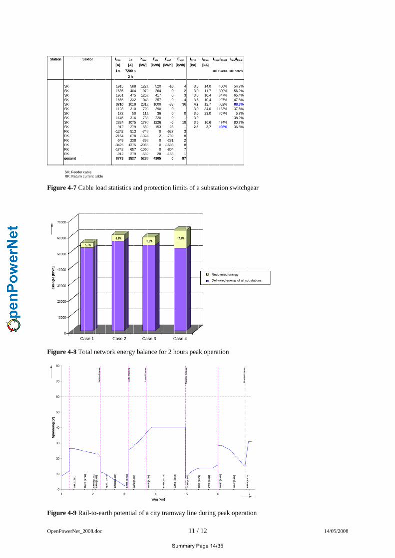
Station Sektor Imax Ieff Pmax Eab Eauf Everl IEinst IKmin IKmin /IEinst Imax/IEinst

[A] [A] [kW] [kWh] [kWh] [kWh] [kA] [kA]

1 s 7200 s soll > 110% soll < 90%

2 h

SK -o.Rämistraße 1915 588 1221 520 -10 4 3,5 14,0 400% 54,7%SK -Seilergraben 1686 404 1072 264 0 2 3,0 11,7 390% 56,2%SK -Hottingerstraße 1961 475 1252 417 0 3 3,0 10,4 347% 65,4%SK -Klosbachstraße 1665 332 1048 257 0 4 3,5 10,4 297% 47,6%SK -Kreuzbühlstraße 3710 1018 2312 1000 -33 36 4,2 12,7 302% 88,3%SK -Heimplatz 1128 310 720 290 0 1 3,0 34,0 1133% 37,6%SK -u.Rämistraße 40 172 50 111 36 0 0 3,0 23,0 767% 5,7%SK -u.Rämistraße 129 1145 316 738 220 0 1 3,0 38,2%SK -Bellevueplatz 2824 1075 1770 1226 -6 18 3,5 16,6 474% 80,7%SK -Zeltweg TB 912 279 582 153 -28 1 2,5 2,7 108% 36,5%RK -Heimplatz 2 Kabel -1242 513 -749 0 -627 3RK -Kreuzbühlstraße -2164 678 -1324 2 -789 8RK -o.Rämistraße -649 238 -393 0 -281 2RK -Heimplatz -3425 1375 -2065 0 -1683 8RK -Bellevueplatz -1742 657 -1050 0 -804 7RK -Zeltweg TB -912 279 -582 28 -153 1gesamt 8773 3527 5289 4305 0 97

SK: SpeisekabelRK: Rückleiterkabel

Pro

men

ade

SK: Feeder cableRK: Return current cable

Figure 4-7 Cable load statistics and protection limits of a substation switchgear

Case 1 Case 2 Case 3 Case 4

Recovered energy

Delivered energy of all substations

Figure 4-8 Total network energy balance for 2 hours peak operation

FR

AN

[6.9

15]

WIN

Z [6

.494

]

WA

RT

[6.0

51]

ZW

IE [5

.691

]

ME

IE [5

.374

]

SC

HT

[4.9

98]

AT

RO

[4.6

02]

EG

UT

[4.2

34]

WA

IF [3

.754

]

WIP

K [3

.297

]

EW

YS

[3.0

63]

DA

MM

[2.6

89]

QU

EL

[2.4

16]

LIM

M [2

.092

]LI

MM

p [2

.003

]

MU

FG

[1.7

32]

SIH

L [1

.391

]

Fra

nk-ä

.Lim

ma

Tob

el-m

_Lim

ma

Lette

-i.Li

mm

a

Lette

-Wip

king

Lette

-o.L

imm

a

0

10

20

30

40

50

60

70

80

1 2 3 4 5 6 7

Weg [km]

Spa

nnun

g [V

]

Figure 4-9 Rail-to-earth potential of a city tramway line during peak operation

Summary Page 14/35


5 Summary

In order to simulate railway power supply networks based on the operation program considering all infrastructu-ral and rolling stock related impacts a new simulation tool called OpenPowerNet was developed by IFB. OpenPowerNet works together with the common Swiss railway operation simulator OpenTrack as a co-simulation. The tasks and properties of the simulation tools can be summarised as follows:

Operation Simulation (OpenTrack) • precise railway operation simulation as a commercial simulator, • co-simulation with the electrical network calculation of OpenPowerNet, • online-communication between operation and electrical network simulation via SOAP-Interface using the

RailML data interchange format, • retroaction of the electrical network conditions to the train driving dynamics within the railway operation

simulation, • automatic disturbance generating caused by the power supply.

Load Flow and Energy Calculation (OpenPowerNet) • complete electrical network calculation reflecting the network structure, the conductor properties and the

electromagnetic coupling effects, • input of the electrical network parameters by use of the geometrical conductor arrangement and the material

properties with unrestricted configuration, • switch status changes of the electrical network during the simulation, • configurable modelling depth for the train propulsion system, • comprehensive analysing and interpreting tools (energy, load flows, currents, voltages, temporal / local) as

well as data export for post-processing.

The main advantage of this solution is the clear separation of the different simulations tasks. On the one hand this allows an independent development and maintenance strategy for both software tools respecting only the interface specification and on the other hand it decreases the modelling effort and the failure possibilities. OpenPowerNet can be used for the entire spectrum of railway power supply systems from DC tramway networks up to AC powered high speed railways. By means of selected simulation results the capability of OpenPowerNet as a new OpenTrack family member could be demonstrated.

Summary Page 15/35

OpenTrack Simulation of Railway Networks

Simulation of Railway Networks

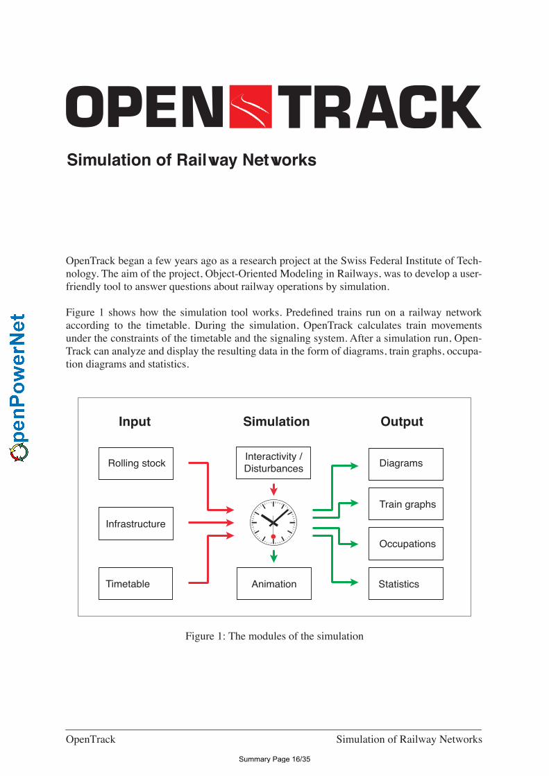
OpenTrack began a few years ago as a research project at the Swiss Federal Institute of Tech-nology. The aim of the project, Object-Oriented Modeling in Railways, was to develop a user-friendly tool to answer questions about railway operations by simulation.

Figure 1 shows how the simulation tool works. Predefined trains run on a railway networkaccording to the timetable. During the simulation, OpenTrack calculates train movementsunder the constraints of the timetable and the signaling system. After a simulation run, Open-Track can analyze and display the resulting data in the form of diagrams, train graphs, occupa-tion diagrams and statistics.

Figure 1: The modules of the simulation

Rolling stock

Infrastructure

Timetable

Input Simulation Output

Diagrams

Train graphs

Occupations

Statistics

Interactivity /Disturbances

Animation

Summary Page 16/35

2


Rolling stock data

OpenTrack stores each locomotive’s technical characteristics, including tractive effort/speeddiagrams, load, length, and adhesion factor. A database organizes locomotives into groups cal-led depots. A simulated train consists of one or more locomotives from a depot together with anumber of passenger or freight cars (carriages or wagons). Another database can store thesimulated train.

Network data

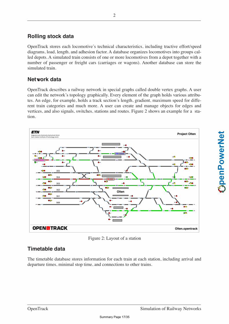
OpenTrack describes a railway network in special graphs called double vertex graphs. A usercan edit the network’s topology graphically. Every element of the graph holds various attribu-tes. An edge, for example, holds a track section’s length, gradient, maximum speed for diffe-rent train categories and much more. A user can create and manage objects for edges andvertices, and also signals, switches, stations and routes. Figure 2 shows an example for a sta-tion.

Figure 2: Layout of a station

Timetable data

The timetable database stores information for each train at each station, including arrival anddeparture times, minimal stop time, and connections to other trains.

355

354

352

351

569

.

353

08

FR10000

RE10003

IC200

Project Olten

Olten.opentrack

Olten

Summary Page 17/35

3


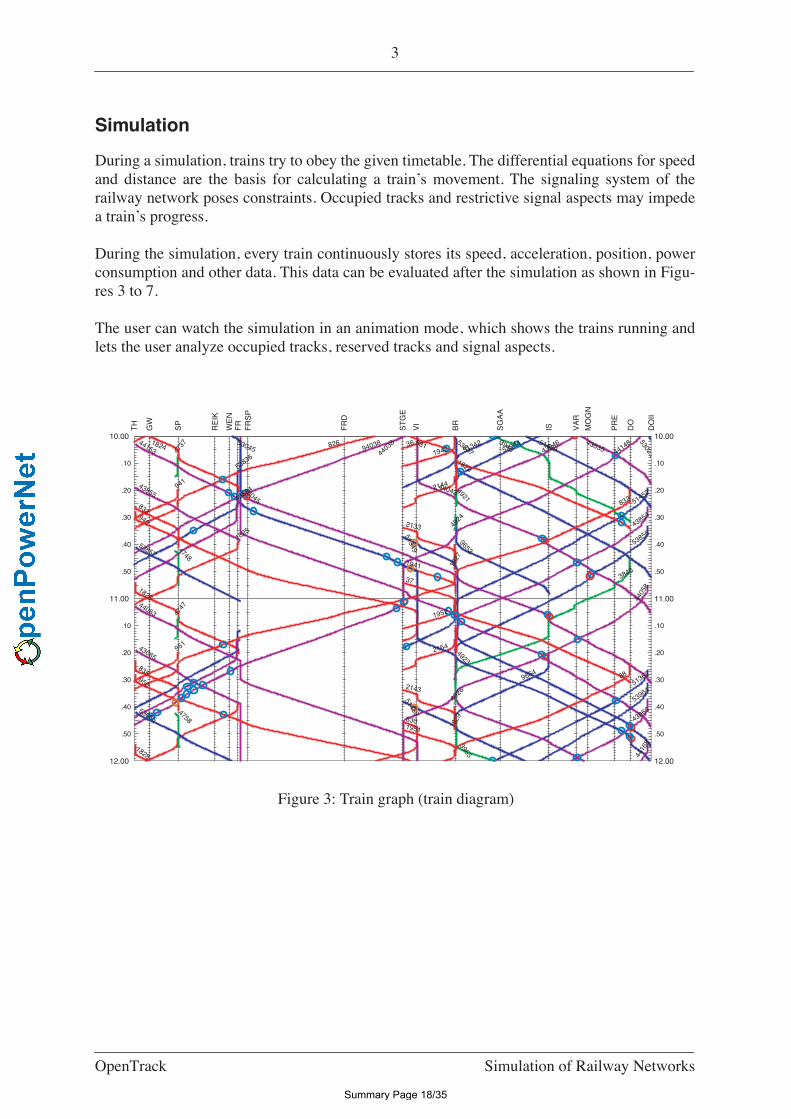
Simulation

During a simulation, trains try to obey the given timetable. The differential equations for speedand distance are the basis for calculating a train’s movement. The signaling system of therailway network poses constraints. Occupied tracks and restrictive signal aspects may impedea train’s progress.

During the simulation, every train continuously stores its speed, acceleration, position, powerconsumption and other data. This data can be evaluated after the simulation as shown in Figu-res 3 to 7.

The user can watch the simulation in an animation mode, which shows the trains running andlets the user analyze occupied tracks, reserved tracks and signal aspects.

Figure 3: Train graph (train diagram)

TH

GW

SP

RE

IK

WE

NF

RF

RS

P

FR

D

ST

GE

VI

BR

SG

AA

IS VA

R

MO

GN

PR

E

DO

DO

II

10.00 10.00

.10 .10

.20 .20

.30 .30

.40 .40

.50 .50

11.00 11.00

.10 .10

.20 .20

.30 .30

.40 .40

.50 .50

12.00 12.00

53837

2133

3945

43065

9653

51452

4383551439

2154

1827

4748

53836

51362

1825

826

1826

43855

3846

951

94038

4747

94143045

940

3965

2144

4737

835

44148

44043

1941

2143

51342

51459

833

1828

53944

4923

51349

4924

4926

4394683118

29

9664

830

53045

950

4405

8

53857

53025

44063

4758

53856

43966

1822

43854

1942

1952

38

43834 4921

37

4415336

4416

8

1951

53964

4403

8

832

53065

1824

Summary Page 18/35

4


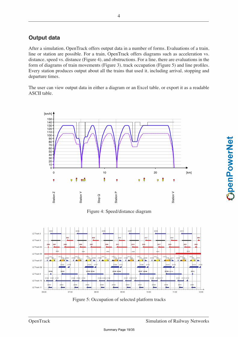
Output data

After a simulation, OpenTrack offers output data in a number of forms. Evaluations of a train,line or station are possible. For a train, OpenTrack offers diagrams such as acceleration vs.distance, speed vs. distance (Figure 4), and obstructions. For a line, there are evaluations in theform of diagrams of train movements (Figure 3), track occupation (Figure 5) and line profiles.Every station produces output about all the trains that used it, including arrival, stopping anddeparture times.

The user can view output data in either a diagram or an Excel table, or export it as a readableASCII table.

Figure 4: Speed/distance diagram

Figure 5: Occupation of selected platform tracks

0 10 20 [km]

0102030405060708090

100110120130140150

[km/h]

Sta

tion

Z

Sta

tion

Y

Sto

p Q

Sta

tion

P

Sta

tion

V

06:00 07:00 08:00 09:00 10:00 11:00 12:00

LZ Track 11

LZ Track 10

LZ Track 9

LZ Track E8

LZ Track E7

LZ Track E6

LZ Track E4

LZ Track 3

LZ Track 2

22301 22351 22303 22353 22305 22355 22307 22357 22309 22359 22311 22361

21100 21201 21101 21203 21203 21105 21205 21205 21109 21207 21207 21113 21209 21209 21117 21211 21211 21121

2210022100 2210122101 2210322103 2210422104 2210522105 2210722107 2210922109 2211122111

21202 21103 21204 21107 21206 21111 21208 21115 21210 21119 21212 21123

21602LAB667

667LAN667

2150LAB2150

LAN215021603 21604 2151

LAB2151

LAN2151670

LAN67021605 21606

LAB671

671LAN671

2154LAB2154

LAN215421607 21608

LAB2155

2155LAN2155

LAB674

674LAN674

21609 21610 675LAB675

LAN675

LAB2158

2158LAN2158

21611 21612LAB2159

2159LAN2159

678LAB678

LAN678

2502 2512

23002300 23012301 23032303 23052305 23072307 23092309 23112311 23132313 23152315 23172317 23192319 23212321 23232323

35513551 35533553 3555 3557 3559 35613561

22001 22003 22005 22007 22009 22011

2210622106 221102210822108

LAB670

2504 251025082506

21613

Summary Page 19/35

5


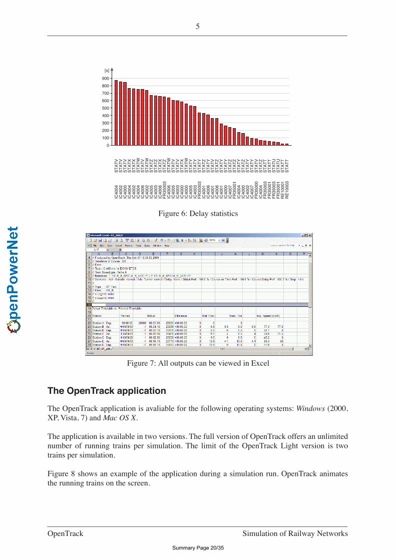
Figure 6: Delay statistics

Figure 7: All outputs can be viewed in Excel

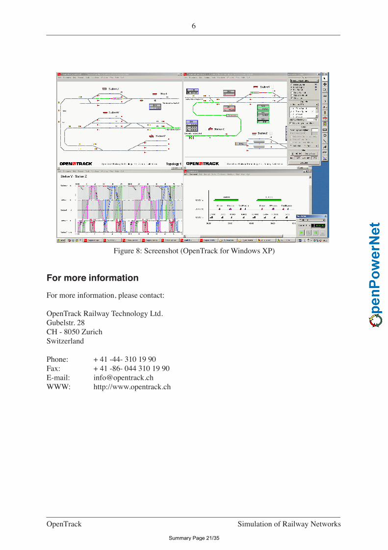
The OpenTrack application

The OpenTrack application is avaliable for the following operating systems:

Windows

(2000,XP, Vista, 7) and

Mac OS X

.

The application is available in two versions. The full version of OpenTrack offers an unlimitednumber of running trains per simulation. The limit of the OpenTrack Light version is twotrains per simulation.

Figure 8 shows an example of the application during a simulation run. OpenTrack animatesthe running trains on the screen.

0

100

200

300

400

500

600

700

800

900

[s]

ST

AT

VS

TA

TV

ST

AT

VS

TA

TX

ST

AT

XS

TA

TW

ST

AT

VS

TA

TW

ST

AT

ZS

TA

TZ

ST

AT

XS

TA

TZ

ST

AT

WS

TA

TV

ST

AT

VS

TA

TX

ST

AT

WS

TA

TY

ST

AT

YS

TA

TY

ST

AT

ZS

TA

TY

ST

AT

VS

TA

TZ

ST

AT

YS

TA

TY

ST

AT

ZS

TA

TZ

ST

AT

YS

TA

TZ

ST

AT

YS

TA

TY

ST

AT

VS

TA

TZ

ST

AT

TS

TA

TT

ST

AT

US

TA

TU

ST

AT

TS

TA

TT

IC40

04IC

4002

IC40

00IC

4004

IC40

02IC

4004

IC40

06IC

4002

IC40

05IC

4003

IC40

06F

R35

003

IC40

06IC

4005

IC40

03IC

4000

IC40

00IC

4005

IC40

03F

R35

003

IC40

01IC

4006

IC40

01IC

4006

IC40

01IC

4000

IC40

07F

R35

001

IC40

04IC

4000

IC40

02IC

4007

FR

3500

0IC

4004

FR

3500

3F

R35

001

FR

3500

3F

R35

001

RE

1000

1R

E10

003

Summary Page 20/35

6


Figure 8: Screenshot (OpenTrack for Windows XP)

For more information

For more information, please contact:

OpenTrack Railway Technology Ltd.Gubelstr. 28CH - 8050 ZurichSwitzerland

Phone: + 41 -44- 310 19 90Fax: + 41 -86- 044 310 19 90E-mail: [email protected]: http://www.opentrack.ch

Summary Page 21/35

Verkehrsbetriebe Zürich Unternehmensbereich Infrastruktur

Luggwegstrasse 65 Postfach 8048 Zürich www.vbz.ch [email protected]

Somchai Yimvuthikul Telefon +41 (0)44 434 48 73 Fax +41 (0)44 432 63 88

IFB Institut für Bahntechnik GmbH Niederlassung Dresden Wiener Str. 114-116 D-01219 Dresden Zürich, 27. August 2010/IPE Bestätigung der Ergebnisse zur Vergleichsmessung mit der OpenPowerNet Simulation Sehr geehrte Damen und Herren Im Rahmen der Netzstudie für die Verkehrsbetriebe Zürich (VBZ) wurde die Überprüfung der Simulationssoftware OpenPowerNet vereinbart. Ziel der Überprüfung war es, auf-grund von Vergleichsmessfahrten die von der Simulationssoftware OpenPowerNet er-zeugten Ergebnisse auf deren Korrektheit hin zu untersuchen. Hierzu wurden drei verschiedene Streckenabschnitte und eine Fahrzeugbauart von den VBZ bestimmt. Diese wurden am Institut für Bahntechnik GmbH (IFB) in Simulations-software OpenPowerNet modelliert und anhand mehrerer typischen Fahrspiele berech-net. Die vom IfB berechneten Fahrspiele bildeten das Fahrprogramm, welches als Basis für die am 21.11.2007 von den VBZ durchgeführten Messfahrten diente. Ein Vergleich der Kennlinien aus den Messfahrten mit denen aus den Simulationen hat ergeben, dass die Effektivwerte der Fahrzeugströme um maximal 6 % abweichen. Dabei ist zu bemerken, dass die während der Messfahrten schwankende Hilfsbetriebe- und Heizungsleistung des Fahrzeugs in der Simulation durch einen konstanten Wert abge-bildet wird. Zudem liessen sich aufgrund von Kraftschlussproblemen nicht alle Messfahr-ten exakt nach den Vorgaben der Simulation nachfahren. Bei der minimalen Spannung am Stromabnehmer ergibt sich in den charakteristischen Fahrspielabschnitten (Fahrzeug mit hohem Leistungsbezug) eine ähnliche Übereinstim-mung. Die Mess- und Simulationskurven liegen bei identischer Stromaufnahme nahezu übereinander. Die Abweichungen liegen stets im Bereich < 5 %. Dies deutet auf die kor-

Summary Page 22/35

2

rekte Hinterlegung des elektrischen Netzmodells hin; die vertraglich geforderten Genau-igkeitsanforderungen sind somit erfüllt. Bei Bremsvorgängen sind Abweichungen zu verzeichnen, die sich jedoch mit den ange-setzten Randbedingungen der Simulation erklären lassen. Während die Fahrzeugsteue-rung die Bremsspannung am Stromabnehmer (aufgrund vorhandener Abnehmer im Netz oder an Bord) immer auf 720 V aufregelt, stellt das Fahrzeugmodell beim Bremsen ohne externe Abnehmer die Spannung auf die Leerlaufspannung des Netzes ein. Energetisch ist dieser Prozess jedoch bedeutungslos, da die dabei im Netz fliessenden Ströme ent-weder nahe oder vollständig Null sind. Aufgrund der erfolgreichen Überprüfung wurde OpenPowerNet als Simulationssoftware für die durchgeführte Netzstudie von den VBZ zugelassen und somit werden die berech-neten Ergebnisse anerkannt. Freundliche Grüsse David Borschberg Leiter Projektierung Bauten

Summary Page 23/35

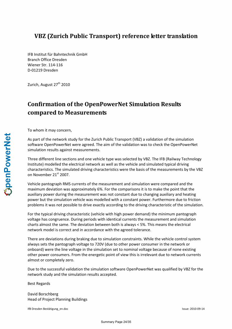
IfB Dresden Bestätigung_en.doc Issue: 2010-09-14

VBZ (Zurich Public Transport) reference letter translation

IFB Institut für Bahntechnik GmbH

Branch Office Dresden

Wiener Str. 114-116

D-01219 Dresden

Zurich, August 27th

2010

Confirmation of the OpenPowerNet Simulation Results

compared to Measurements

To whom it may concern,

As part of the network study for the Zurich Public Transport (VBZ) a validation of the simulation

software OpenPowerNet were agreed. The aim of the validation was to check the OpenPowerNet

simulation results against measurements.

Three different line sections and one vehicle type was selected by VBZ. The IFB (Railway Technology

Institute) modelled the electrical network as well as the vehicle and simulated typical driving

characteristics. The simulated driving characteristics were the basis of the measurements by the VBZ

on November 21st

2007.

Vehicle pantograph RMS currents of the measurement and simulation were compared and the

maximum deviation was approximately 6%. For the comparisons it is to make the point that the

auxiliary power during the measurement was not constant due to changing auxiliary and heating

power but the simulation vehicle was modelled with a constant power. Furthermore due to friction

problems it was not possible to drive exactly according to the driving characteristic of the simulation.

For the typical driving characteristic (vehicle with high power demand) the minimum pantograph

voltage has congruence. During periods with identical currents the measurement and simulation

charts almost the same. The deviation between both is always < 5%. This means the electrical

network model is correct and in accordance with the agreed tolerance.

There are deviations during braking due to simulation constraints. While the vehicle control system

always sets the pantograph voltage to 720V (due to other power consumer in the network or

onboard) were the line voltage in the simulation set to nominal voltage because of none existing

other power consumers. From the energetic point of view this is irrelevant due to network currents

almost or completely zero.

Due to the successful validation the simulation software OpenPowerNet was qualified by VBZ for the

network study and the simulation results accepted.

Best Regards

David Borschberg

Head of Project Planning Buildings

Summary Page 24/35

Summary Page 25/35

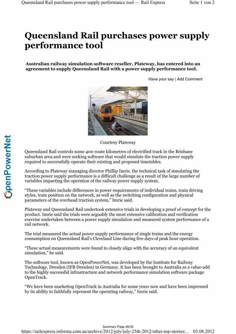
Queensland Rail purchases power supply performance tool

Australian railway simulation software reseller, Plateway, has entered into an agreement to supply Queensland Rail with a power supply performance tool.

Have your say | Add Comment

Courtesy Plateway

Queensland Rail controls some 400 route kilometres of electrified track in the Brisbane suburban area and were seeking software that would simulate the traction power supply required to successfully operate their existing and proposed timetables.

According to Plateway managing director Phillip Imrie, the technical task of simulating the traction power supply performance is a difficult challenge as a result of the large number of variables impacting the operation of the railway power supply system.

“These variables include differences in power requirements of individual trains, train driving styles, train position on the network, as well as the switching configuration and physical parameters of the overhead traction system,” Imrie said.

Plateway and Queensland Rail undertook extensive trials in developing a proof of concept for the product. Imrie said the trials were arguably the most extensive calibration and verification exercise undertaken between a power supply simulation and measured system performance of a rail network.

The trial measured the actual power supply performance of single trains and the energy consumption on Queensland Rail’s Cleveland Line during five days of peak hour operation.

“These actual measurements were found to closely align with the accuracy of an equivalent simulation,” he said.

The software tool, known as OpenPowerNet, was developed by the Institute for Railway Technology, Dresden (IFB Dresden) in Germany. It has been brought to Australia as a value-add to the highly successful infrastructure and network performance simulation software package OpenTrack.

“We have been marketing OpenTrack in Australia for some years now and have been impressed by its ability to faithfully represent the operating railway," Imrie said.

Seite 1 von 2Queensland Rail purchases power supply performance tool — Rail Express

03.08.2012https://railexpress.informa.com.au/archive/2012/july/july-25th-2012/other-top-stories/...Summary Page 26/35

"OpenPowerNet allows us to now test power supplies to the railway as part of a co-simulation exercise and will allow users to accurately assess the potential of their existing and proposed infrastructure."

Germany’s IFB Dresden wished to create a plug-in simulation module using the advantages of an existing commercial railway operation simulator. OpenTrack was chosen as the ideal tool due to its excellent capability and relative ease of use.

OpenTrack deals with the rail network simulation under normal and disturbed timetable situations using the infrastructure and train data. In a synchronised simulation, OpenPowerNet can present an energy prognosis of the entire electrified railway taking into account engine and train power consumption and location within the network.

OpenPowerNet is already used in Europe and China for the simulation of both AC and DC railway traction systems and is considered one of the most advanced software tools for this purpose on the market.

On the new Netherlands high speed Line Zuid, it is used for the commercial train energy billing of different train operators. For Chinese high speed lines, it has been used to test the rating of the current return system. The analysis and optimisation of the Zurich Tram and Trolley bus power supply network is also done using OpenPowerNet.

The tool has been purchased by Queensland Rail to allow proof of new design concepts, analysis of their existing system performance, and to improve their investment decision making.

A full technical paper on OpenPowernet has been submitted for inclusion in AusRAIL 2012, to be held in Canberra in November.

Seite 2 von 2Queensland Rail purchases power supply performance tool — Rail Express

03.08.2012https://railexpress.informa.com.au/archive/2012/july/july-25th-2012/other-top-stories/...Summary Page 27/35

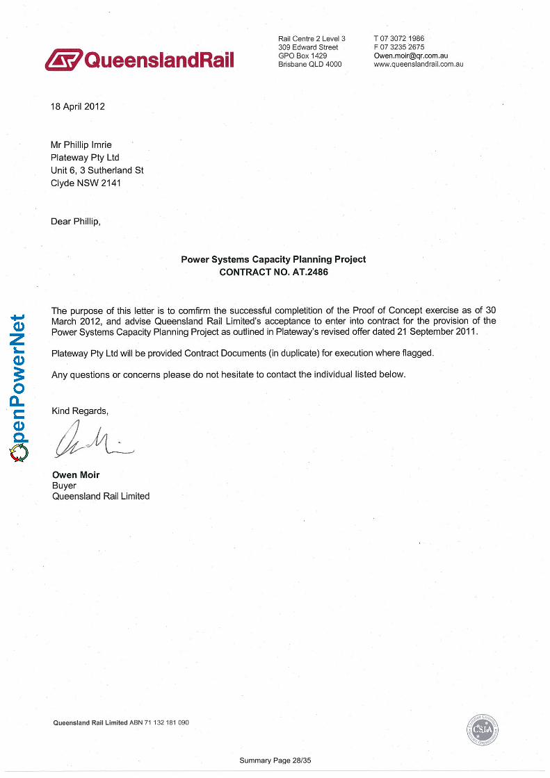
Summary Page 28/35

Summary Page 29/35

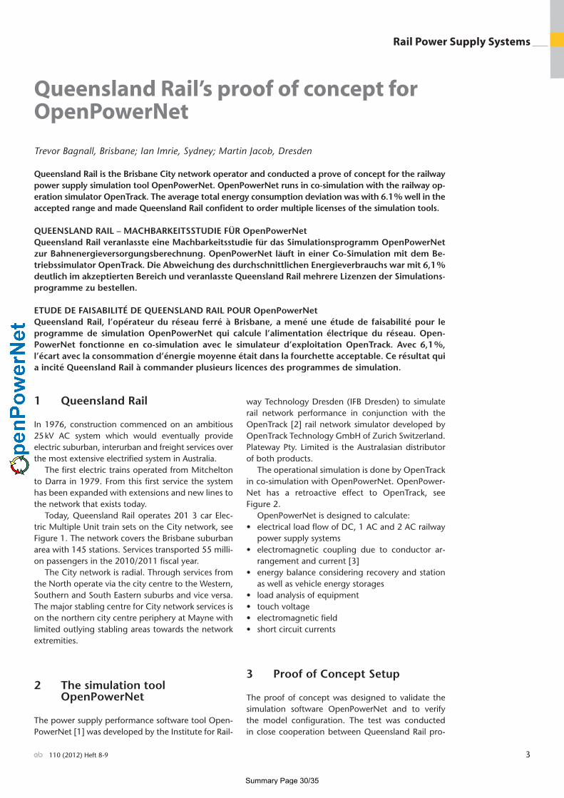
3110 (2012) Heft 8-9

Rail Power Supply Systems

Queensland Rail’s proof of concept for OpenPowerNet

Trevor Bagnall, Brisbane; Ian Imrie, Sydney; Martin Jacob, Dresden

Queensland Rail is the Brisbane City network operator and conducted a prove of concept for the railway power supply simulation tool OpenPowerNet. OpenPowerNet runs in co-simulation with the railway op-eration simulator OpenTrack. The average total energy consumption deviation was with 6.1 % well in the accepted range and made Queensland Rail confi dent to order multiple licenses of the simulation tools.

QUEENSLAND RAIL – MACHBARKEITSSTUDIE FÜR OpenPowerNetQueensland Rail veranlasste eine Machbarkeitsstudie für das Simulationsprogramm OpenPowerNet zur Bahnenergieversorgungsberechnung. OpenPowerNet läuft in einer Co-Simulation mit dem Be-triebssimulator OpenTrack. Die Abweichung des durchschnittlichen Energieverbrauchs war mit 6,1 % deutlich im akzeptierten Bereich und veranlasste Queensland Rail mehrere Lizenzen der Simulations-programme zu bestellen.

ETUDE DE FAISABILITÉ DE QUEENSLAND RAIL POUR OpenPowerNetQueensland Rail, l’opérateur du réseau ferré à Brisbane, a mené une étude de faisabilité pour le programme de simulation OpenPowerNet qui calcule l’alimentation électrique du réseau. Open-PowerNet fonctionne en co-simulation avec le simulateur d’exploitation OpenTrack. Avec 6,1 %, l’écart avec la consommation d’énergie moyenne était dans la fourchette acceptable. Ce résultat qui a incité Queensland Rail à commander plusieurs licences des programmes de simulation.

1 Queensland Rail

In 1976, construction commenced on an ambitious 25 kV AC system which would eventually provide electric suburban, interurban and freight services over the most extensive electrifi ed system in Australia.

The fi rst electric trains operated from Mitchelton to Darra in 1979. From this fi rst service the system has been expanded with extensions and new lines to the network that exists today.

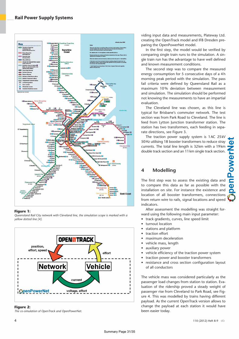
Today, Queensland Rail operates 201 3 car Elec-tric Multiple Unit train sets on the City network, see Figure 1. The network covers the Brisbane suburban area with 145 stations. Services transported 55 milli-on passengers in the 2010/2011 fi scal year.

The City network is radial. Through services from the North operate via the city centre to the Western, Southern and South Eastern suburbs and vice versa. The major stabling centre for City network services is on the northern city centre periphery at Mayne with limited outlying stabling areas towards the network extremities.

2 The simulation tool OpenPower Net

The power supply performance software tool Open-PowerNet [1] was developed by the Institute for Rail-

way Technology Dresden (IFB Dresden) to simulate rail network performance in conjunction with the OpenTrack [2] rail network simulator developed by OpenTrack Technology GmbH of Zurich Switzerland. Plateway Pty. Limited is the Australasian distributor of both products.

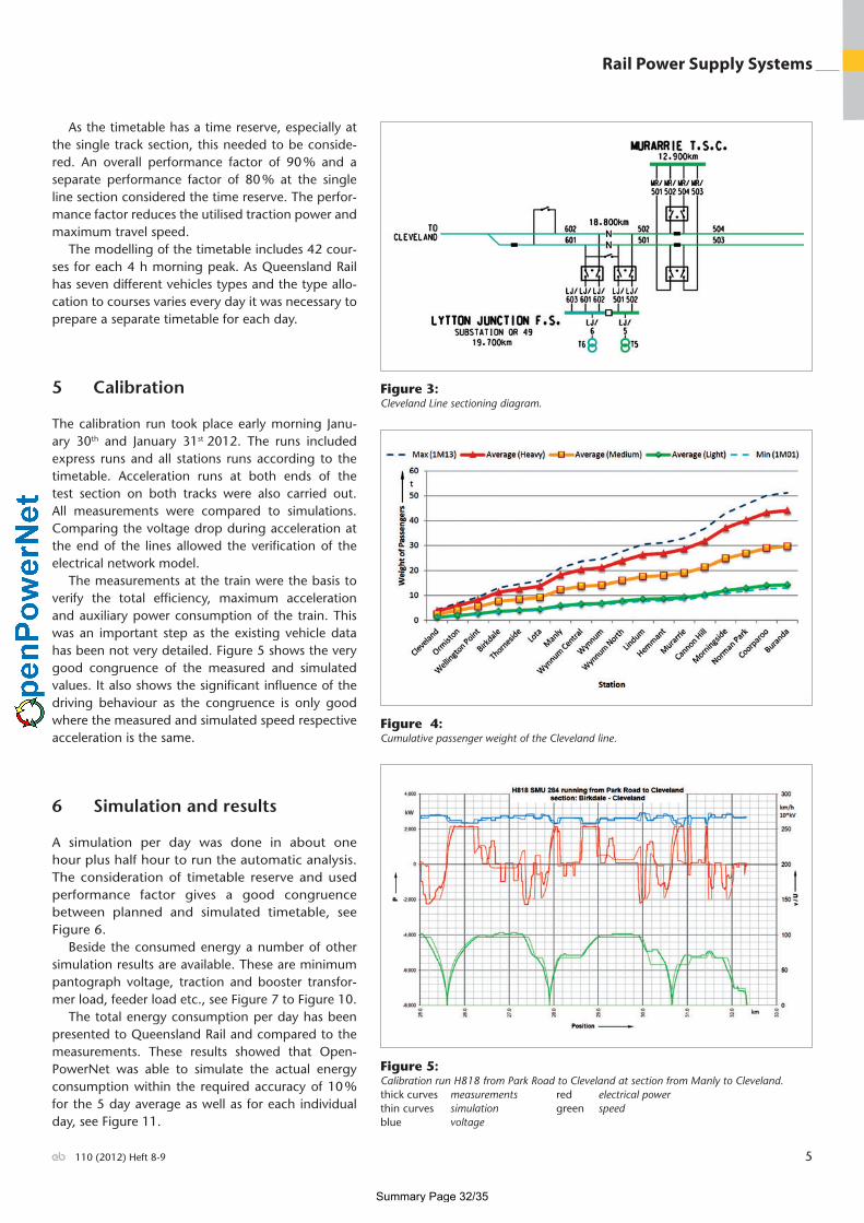
The operational simulation is done by OpenTrack in co-simulation with OpenPowerNet. OpenPower-Net has a retroactive effect to OpenTrack, see Fig ure 2.

OpenPowerNet is designed to calculate:• electrical load fl ow of DC, 1 AC and 2 AC railway

power supply systems• electromagnetic coupling due to conductor ar-

rangement and current [3]• energy balance considering recovery and station

as well as vehicle energy storages• load analysis of equipment• touch voltage• electromagnetic fi eld• short circuit currents

3 Proof of Concept Setup

The proof of concept was designed to validate the simulation software OpenPowerNet and to verify the model confi guration. The test was conducted in close cooperation between Queensland Rail pro-

Summary Page 30/35

4 110 (2012) Heft 8-9


viding input data and measurements, Plateway Ltd. creating the OpenTrack model and IFB Dresden pre-paring the OpenPowerNet model.

In the fi rst step, the model would be verifi ed by comparing single train runs to the simulation. A sin-gle train run has the advantage to have well defi ned and known measurement conditions.

The second step was to compare the measured energy consumption for 5 consecutive days of a 4 h morning peak period with the simulation. The pass fail criteria were defi ned by Queensland Rail as a maximum 10 % deviation between measurement and simulation. The simulation should be performed not knowing the measurements to have an impartial evaluation.

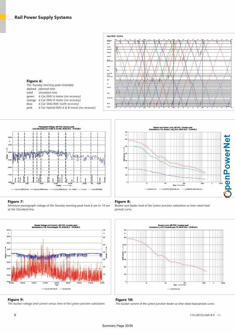
The Cleveland line was chosen, as this line is typical for Brisbane’s commuter network. The test section was from Park Road to Cleveland. The line is feed from Lytton Junction transformer station. The station has two transformers, each feeding in sepa-rate directions, see Figure 3.

The traction power supply system is 1 AC 25 kV 50 Hz utilising 18 booster transformers to reduce stray currents. The total line length is 32 km with a 19 km double track section and an 11 km single track section.

4 Modelling

The fi rst step was to assess the existing data and to compare this data as far as possible with the installation on site. For instance the existence and location of all booster transformers, connections from return wire to rails, signal locations and speed indicators.

After assessment the modelling was straight for-ward using the following main input parameter:• track gradients, curves, line speed limit• turnout location• stations and platform• traction effort• maximum deceleration• vehicle mass, length• auxiliary power• vehicle effi ciency of the traction power system• traction power and booster transformers• resistance and cross section confi guration layout

of all conductors

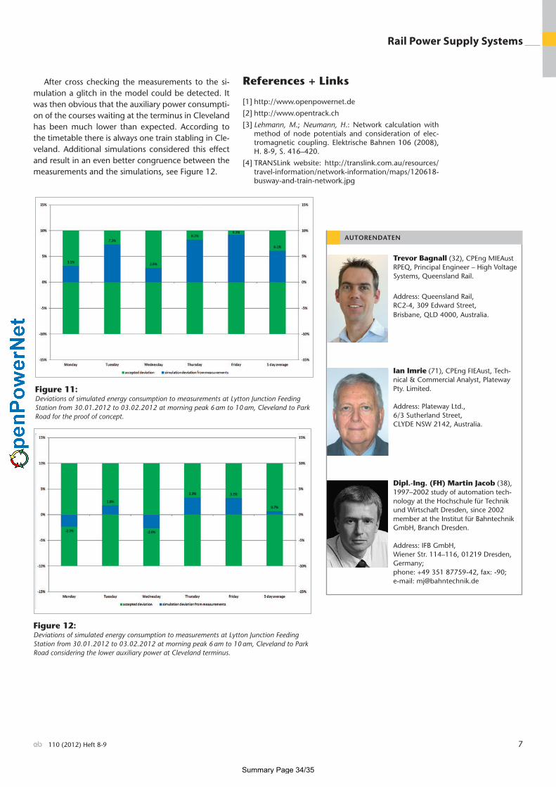
The vehicle mass was considered particularly as the passenger load changes from station to station. Eva-luation of the ridership proved a steady weight of passenger rise from Cleveland to Park Road, see Fig-ure 4. This was modelled by trains having different payload. As the current OpenTrack version allows to change the payload at each station it would have been easier today.

Figure 1: Queensland Rail City network with Cleveland line, the simulation scope is marked with a yellow dotted line [4].

Figure 2: The co-simulation of OpenTrack and OpenPowerNet.

Summary Page 31/35

5110 (2012) Heft 8-9


Figure 4:Cumulative passenger weight of the Cleveland line.

Figure 5: Calibration run H818 from Park Road to Cleveland at section from Manly to Cleveland.thick curves measurements red electrical powerthin curves simulation green speedblue voltage

Figure 3: Cleveland Line sectioning diagram.

As the timetable has a time reserve, especially at the single track section, this needed to be conside-red. An overall performance factor of 90 % and a separate performance factor of 80 % at the single line section considered the time reserve. The perfor-mance factor reduces the utilised traction power and maximum travel speed.

The modelling of the timetable includes 42 cour-ses for each 4 h morning peak. As Queensland Rail has seven different vehicles types and the type allo-cation to courses varies every day it was necessary to prepare a separate timetable for each day.

5 Calibration

The calibration run took place early morning Janu-ary 30th and January 31st 2012. The runs included express runs and all stations runs according to the timetable. Acceleration runs at both ends of the test section on both tracks were also carried out. All measurements were compared to simulations. Comparing the voltage drop during acceleration at the end of the lines allowed the verifi cation of the electrical network model.

The measurements at the train were the basis to verify the total effi ciency, maximum acceleration and auxiliary power consumption of the train. This was an important step as the existing vehicle data has been not very detailed. Figure 5 shows the very good congruence of the measured and simulated values. It also shows the signifi cant infl uence of the driving behaviour as the congruence is only good where the measured and simulated speed respective acceleration is the same.

6 Simulation and results

A simulation per day was done in about one hour plus half hour to run the automatic analysis. The consideration of timetable reserve and used performance factor gives a good congruence between planned and simulated timetable, see Figure 6.

Beside the consumed energy a number of other simulation results are available. These are minimum pantograph voltage, traction and booster transfor-mer load, feeder load etc., see Figure 7 to Figure 10.

The total energy consumption per day has been presented to Queensland Rail and compared to the measurements. These results showed that Open-PowerNet was able to simulate the actual energy consumption within the required accuracy of 10 % for the 5 day average as well as for each individual day, see Figure 11.

Summary Page 32/35

6 110 (2012) Heft 8-9


Figure 6: The Tuesday morning peak timetable.dashed planned timesolid simulated timegreen 6 Car EMU 6 motor (no recovery)orange 6 Car EMU 8 motor (no recovery)blue 6 Car SMU/IMU (with recovery)pink 6 Car Hybrid EMU 6 & 8 motor (no recovery)

Figure 7: Minimum pantograph voltage of the Tuesday morning p eak from 6 am to 10 am at the Cleveland line.

Figure 8: Busbar and feeder load of the Lytton Junction substat ion as time rated load periods curve.

Figure 9: The busbar voltage and current versus time of the Lyt ton Junction substation.

Figure 10: The busbar current of the Lytton Junction feeder as time rated load periods curve.

Summary Page 33/35

7110 (2012) Heft 8-9


AUTORENDATEN

Trevor Bagnall (32), CPEng MIEAust RPEQ, Principal Engineer – High Voltage Systems, Queensland Rail.

Address: Queensland Rail, RC2-4, 309 Edward Street, Brisbane, QLD 4000, Australia.

Ian Imrie (71), CPEng FIEAust, Tech-nical & Commercial Analyst, Plateway Pty. Limited.

Address: Plateway Ltd., 6/3 Sutherland Street, CLYDE NSW 2142, Australia.

Dipl.-Ing. (FH) Martin Jacob (38), 1997–2002 study of automation tech-nology at the Hochschule für Technik und Wirtschaft Dresden, since 2002 member at the Institut für Bahntechnik GmbH, Branch Dresden.

Address: IFB GmbH, Wiener Str. 114–116, 01219 Dresden, Germany; phone: +49 351 87759-42, fax: -90; e-mail: [email protected]

Figure 11: Deviations of simulated energy consumption to measur ements at Lytton Junction Feeding Station from 30.01.2012 to 03.02.2012 at morning peak 6 am to 10 am, Cleveland to Park Road for the proof of concept.

Figure 12: Deviations of simulated energy consumption to measureme nts at Lytton Junction Feeding Station from 30.01.2012 to 03.02.2012 at morning peak 6 am to 10 am, Cleveland to Park Road considering the lower auxiliary power at Cleveland terminus.

After cross checking the measurements to the si-mulation a glitch in the model could be detected. It was then obvious that the auxiliary power consumpti-on of the courses waiting at the terminus in Cleveland has been much lower than expected. According to the timetable there is always one train stabling in Cle-veland. Additional simulations considered this effect and result in an even better congruence be tween the measurements and the simulations, see Figure 12.

References + Links

[1] http://www.openpowernet.de

[2] http://www.opentrack.ch

[3] Lehmann, M.; Neumann, H.: Network calculation with method of node potentials and consideration of elec-tromagnetic coupling. Elektrische Bahnen 106 (2008), H. 8-9, S. 416–420.

[4] TRANSLink website: http://translink.com.au/resources/travel-information/network-information/maps/120618-busway-and-train-network.jpg

Summary Page 34/35

Contact details:

IFB Institut für Bahntechnik GmbH

(Institute of Railway Technology)

Branch Office Dresden

Wiener Straße 114 – 116

D – 01219 Dresden

Fon: +49 351 / 877 59 – 0

Fax: +49 351 / 877 59 – 90

Mail: [email protected]

http://www.openpowernet.de

http://www.bahntechnik.de

Contact:

Dipl.-Ing. (FH) Martin Jacob +49 351 / 877 59 – 42

Dipl.-Ing. (FH) Harald Scheiner +49 351 / 877 59 – 62

Summary Page 35/35

Documents

Simulation of Railway Power Supply Systems - …openpowernet.de/downloads/summary/OPN_OT_summary_en.pdf · Simulation of . Railway Power Supply Systems . in Co-Simulation with . Program