Simulation of the Landfall of the Deepwater Horizon Oil on theShorelines of the Gulf of MexicoMichel C. Boufadel,*,† Ali Abdollahi-Nasab,† Xiaolong Geng,† Jerry Galt,‡ and Jagadish Torlapati†

†Center for Natural Resources Development and Protection, Department of Civil and Environmental Engineering, New JerseyInstitute of Technology, Newark, New Jersey 07102, United States‡Genwest Systems, Incorporated, Edmonds, Washington 98020, United States

*S Supporting Information

ABSTRACT: We conducted simulations of oil transport from the footprint of theMacondo Well on the water surface throughout the Gulf of Mexico, includingdeposition on the shorelines. We used the U.S. National Oceanic AtmosphericAdministration (NOAA) model General NOAA Operational Modeling Environ-ment (GNOME) and the same parameter values and input adopted by NOAAfollowing the Deepwater Horizon (DWH) blowout. We found that thedisappearance rate of oil off the water surface was most likely around 20% perday based on satellite-based observations of the disappearance rate of oil detectedon the sea surface after the DWH wellhead was capped. The simulations and oilmass estimates suggest that the mass of oil that reached the shorelines was between10 000 and 30 000 tons, with an expected value of 22 000 tons. More than 90% ofthe oil deposition occurred on the Louisiana shorelines, and it occurred in twobatches. Simulations revealed that capping the well after 2 weeks would haveresulted in only 30% of the total oil depositing on the shorelines, while cappingafter 3 weeks would have resulted in 60% deposition. Additional delay in capping after 3 weeks would have averted littleadditional shoreline oiling over the ensuing 4 weeks.

■ INTRODUCTION

The Deepwater Horizon (DWH) well blowout in the Gulf ofMexico (GOMEX) released oil from April 20th until capped onJuly 15th, 2013. The amount of oil released was estimated ataround 5 million barrels.1 Despite the considerable resourcesand effort marshaled to prevent the oil from reaching theshorelines, the spill contaminated around 500 km of shorelines(Figure 1) in the categories of heavy and moderate.2,3 Impactsthat included damage to wetlands and the fishing and touristindustries were highlighted in a recent report.4 This paperaddresses only the deposition of oil on the shorelines, becausenear shore open waters and shorelines constitute highlyproductive regions both ecologically and economically and,because oil tends to persist in shorelines in comparison to openwater,5−8 which tends to prolong the impact on the economyand ecology of shorelines. The persistence of oil also increasesthe remediation cost by orders of magnitude in comparison tooil intercepted at sea. Thus, it is important to develop a betterunderstanding of the movement of oil and its deposition ontothe shorelines.There are numerous works on the modeling of the

hydrodynamics and transport in the GOMEX.9−19 Paris etal.16 predicted the movement of oil from 1200 m deep using adetailed three-dimensional (3D) fate and transport that focusedon the subsurface transport. Le Henaff et al.18 complementedthe work by Paris et al.16 by focusing on oil transport on thewater surface and found that the wind played a major role in

advecting the oil to the northern GOMEX. Kourafalou andAndroulidakis17 conducted a rigorous study for the 3Dtransport of oil near the Mississippi Delta and evaluated theinfluence of the river diversion conducted to minimize oilintrusion inland.4,20 Barker15 conducted Monte Carlo simu-lations consisting of 500 individual oil trajectory scenarios usinghistorical data of water currents and winds. The results byBarker15 indicated that, in approximately 75% of the scenarios,oil would be transported out of the GOMEX by the LoopCurrent. This means that the actual trajectory of oil from theDWH falls in the 25% of scenarios.Our goal herein is to quantify the amount of oil that reached

the shorelines. We make two major assumptions in ourinvestigation. First, we assume that the only source of oil to theshoreline is the oil that reached the surface immediately abovethe wellhead (known as Mississippi Canyon 252, MC252 forshort). This assumption is justified by the fact that the mainpart of the plume that rose to the surface occurred within 1.5km of the well head projection on the water surface.21 Inaddition, as the subsurface plume migrated 200 km horizontallyat an approximate depth of 1200 m, it became diluted anddensity stratification prevented it from rising to the surface.22 In

Received: March 19, 2014Revised: June 30, 2014Accepted: July 28, 2014Published: July 28, 2014

Article

pubs.acs.org/est

© 2014 American Chemical Society 9496 dx.doi.org/10.1021/es5012862 | Environ. Sci. Technol. 2014, 48, 9496−9505

Terms of Use

addition, droplets that were small enough to be advected in thedeep plume have a rise time to the surface varying from weeksto months,21 a time scale over which biodegradation could playa major role.23,24 Second, we assume that response efforts(skimming, burning, and dispersant application) did not alterthe spatial distribution of the oil reaching the shoreline but onlyreduced the amount of oil reaching the shorelines; because ofthe large size of the spill, it was not possible to set asideresources to protect a particular area of the shoreline. Ratherresources were marshaled to intercept oil whenever it wasfound. This second assumption is needed because detailed dataon the amount of oil removed at particular locations aredifficult to compile and evaluate. Considering the uncertainty inoil trajectory, this assumption is plausible.

■ BACKGROUND

Oil on the water surface becomes transported by winds,waves,25−27 and sea currents. These processes are simulatedsuccinctly in the National Oceanic and Atmospheric Admin-istration (NOAA) General NOAA Operational ModelingEnvironment (GNOME), which moves Lagrangian elements,labeled “splots” on the water surface based on input of seacurrents obtained from hydrodynamic models (structured orunstructured grids) and wind models. For the latter, GNOMErequires a “windage factor”, which reflects the surface watermovement as a percentage of the wind speed. The windagefactor is typically around 3% of the wind speed and is usuallyless than 6% of the wind speed.28 The GNOME model alsoassigns a turbulent diffusion coefficient to represent turbulentmixing.During the DWH blowout, the Environmental Response

Division (ERD) of the Office of Response and Restoration atNOAA relied on six available hydrodynamic models to predictthe movement of oil, as reported by MacFadyen et al.29 Oneach day, the NOAA ERD selected the hydrodynamic modelthat matched best the observations obtained from satellites andoverflights29 (see Tables S1 and S2 of the Supporting

Information). The wind data were derived from the NationalWeather Service gridded products.29 The NOAA ERDsimulated the oil for 72 h and initialized the oil distributiontwice a day in the first few weeks of the spill and later daily.29

The initialization was performed on the basis of observations.

■ METHOD OF APPROACH

Our goal was to simulate the continuous release of oil at thewater surface and its subsequent transport and fate on the watersurface until it reached the shorelines, including barrier islands.The overall oil spill evaluation is modeled as follows: In oursimulations, we released 500 splots at the water surface dailyuntil the date of well capping. These splots represent theaverage amount of oil released to the water surface per day.These splots were then tracked throughout the GOMEX untillandfall (or beaching). The number of splots released to thewater surface immediately above the wellhead does notrepresent any particular oil volume; it could represent 33 000barrels per day (bpd), as estimated by Barker,15 or only 1000bpd. The main thrust of this investigation is to evaluate theportion of the released oil at the sea surface that reaches theshorelines (including the barrier islands). We used theparameter values and the water current and wind input usedby NOAA ERD during the DWH spill. This information wasretrieved from the database of the NOAA ERD archives.GNOME has an option for the landfall (i.e., beaching) and

resuspension of oil. We considered the deposition only, because(1) the net movement of floating materials on beaches islandward,30 (it is thus unlikely for a large portion of thedeposited oil to move seaward if it becomes resuspended) and(2) the accuracy of the hydrodynamic models used in this studydeteriorates in the coastal zone because of coarseness of thegrid and the fact that these models were developed primarilyfor offshore hydrodynamics and transport. Therefore, there wasno justification for a detailed mechanistic model of depositionand resuspension of oil on the shorelines. Le Henaff et al.18

assumed that oil becomes deposited when it is within 3 m from

Figure 1.Map of region of shorelines affected by the actual spill (http://www.nytimes.com/interactive/2010/05/27/us/20100527-oil-landfall.html).The darker red indicates heavier shoreline oiling. The gray region shows the suspected satellite-derived surface oiling over the entire spill period.

Environmental Science & Technology Article

dx.doi.org/10.1021/es5012862 | Environ. Sci. Technol. 2014, 48, 9496−95059497

the bottom, and they did not consider resuspension of oil afterdeposition.Oil is expected to disappear off the surface because of a

variety of mechanisms, including evaporation, photooxidation,dissolution, emulsion, and biodegradation.31,32 In addition, oilcould deplete off the surface through entrainment into thewater column as droplets (labeled as “dispersion” in the oilliterature because the oil “disperses” into small droplets)because of waves27 and Langmuir cells.33,34 However, only oilthat does not return to the surface should be considered as“disappeared” off the surface. This “lost” oil mass in the watercolumn is usually made up of small oil droplets, typically lessthan 100 μm in diameter.35 Furthermore, oil disappeared offthe surface due to active removal by response activities thatincluded skimming, dispersion, and in situ burning.36,37

The NOAA’s ERD was interested in providing the “worstcase scenario” for the response officials and was reinitializingthe spatial distribution of oil every 24 h based on observationsfrom satellites and overflights; it did not consider the depletionof oil from the surface.29 However, oil depletion off the surfaceneeds to be considered when simulating the continuous fate ofoil during 3 months. Rigorously accounting for each of theaforementioned factors of oil weathering is not realistic becauseof the complexity and scale of the oil−water−atmospheresystem. However, one could deduce the oil depletion rate offthe surface based on empirical observation as follows.Figure 2 depicts the areal coverage of oil based on satellite

data obtained from the date of well capping (i.e., July 15th)

until July 30th. The areal extent fluctuated but a trend ofdecrease is obvious, resulting in complete depletion of the oiloff the water surface. Obviously, patches of oil persisted forlonger durations, but their areal extents and masses arenegligible in comparison. The bulk of the oil slick was relativelyfar from the shorelines, as confirmed from satellite andsimulation data between July 15th and August 5th. It is thusreasonable to assume that the disappearance of oil from thesurface was not due to beaching but weathering and activeremoval by the response activites.An expedient model for the depletion of fields (mass, surface

area, etc.) is an exponential decay curve, used herein for theoiled area

= −At

kAdd (1)

where A is the area of oiled water surface (km2) and k is a first-order rate (day−1).The model GNOME does not allow for depletion of mass;

rather, it reduces the portion of components in a mixture ofhydrocarbons. For this reason, the removal of a selectedpercentage (20% for k = 0.2 day−1 and 10% for k = 0.1 day−1)of the splots was conducted as follows: (1) Run the model for24 h. (2) Output the results (e.g., number and location of oilsplots). (3) Postprocess the results to separate the splots thatbeached from those that remained on the water surface. (4)Use a uniform random generator to remove randomly theselected percentage of the splots off the water surface. (5) Usethe beached splots and those that “survived” on the watersurface as the initial condition for splots for a GNOMEsimulation for another 24 h. Note that beached splots do notdeplete nor do they move, and the splots that survive continuetheir transport on the water surface unaffected. (6) Repeat theprocess until there are no splots on the water surface or for 3weeks after capping, whichever occurs first.

■ RESULTSFigure 2 shows that fitting eq 1 to the observed oiled areastarting on July 20th, the largest oiled area after well capping,gave k = 0.2 day−1, (i.e., the oiled area shrinks by 20% daily).The fit starting on July 15th (the date of the well capping) gavek = 0.11 day−1, and we adopted k = 0.1 day−1 for simplicity. Thefit giving k = 0.2 day−1 was better than that giving k = 0.1 day−1.Nevertheless, we conducted simulations with k = 0.2, 0.1, and0.0 day−1 (i.e., no depletion). For all of the simulations, we usedthe same windage factors used by NOAA ERD daily, whichvaried between 0 and 3%. We also used the same value of thehorizontal turbulent diffusion coefficient as NOAA ERD, 10m2/s, because we found this value reasonable (see, for example,the study by Boufadel et al.26 for a discussion on the horizontaldiffusion coefficient).Panels a, b, and c of Figure 3 report the simulated splots

distribution on August 5th, 2010 based on k = 0.2, 0.1, and 0.0day−1, respectively. The oil deposition on the shorelines inFigure 3a (k = 0.2 day−1) appears by far to have the closestresemblance to the observed oil deposition on the shorelines(Figure 1). Panels b and c of Figure 3 show considerable oildeposition west of longitude −91, which is in disagreementwith observation (Figure 1). Also, around the location (−88.6,30.4) (i.e., on the shorelines of Mississippi), Figure 3a agreesclosest with observations (Figure 1), while panels b and c ofFigure 3 result in a large oil deposition. Because of the decreasein resolution near the shorelines, GNOME simulations inembayments should not be considered accurate and, thus,should not be compared to observations there. There aresituations where the model provided no deposition, whereasdeposition actually occurred, such as, for example, at CatIsland.38 However, given that the size of the computationalblock of the hydrodynamic model is 10 × 10 km, it is likely thatsome areas at smaller spatial scales may not be accuratelyportrayed.Using k = 0.2 day−1, we provide in Figure 4 further

comparison of the model to data obtained from overflight andsatellite observation.39−41 Figure 4a shows that the modelpredicted the presence of two plumes on May 7th, 2010: oneextending west of MC252 and another in the northern part of

Figure 2. Observed areal extent of surface oil and two fittedexponential decay curves. The observed areal extent was obtained fromNOAA/National Environmental Satellite, Data, and InformationService (NESDIS) (http://www.ssd.noaa.gov/PS/MPS/deepwater.html).

Environmental Science & Technology Article

dx.doi.org/10.1021/es5012862 | Environ. Sci. Technol. 2014, 48, 9496−95059498

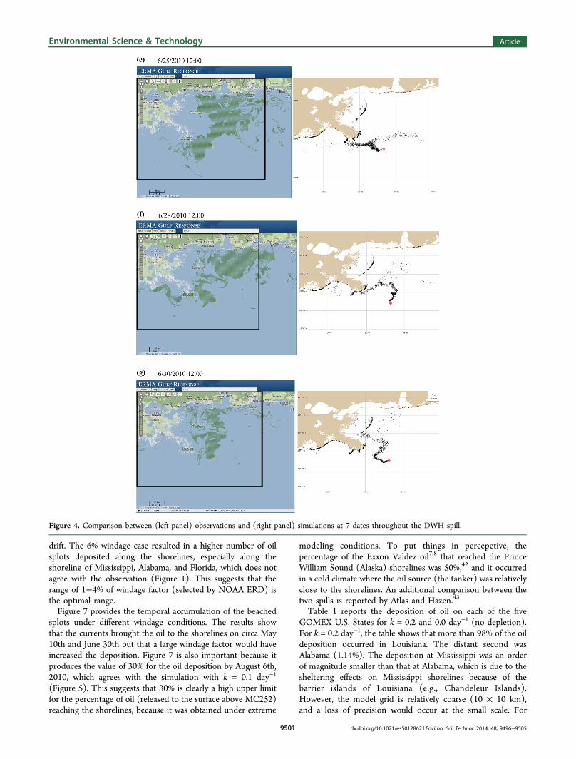
the GOMEX. The predicted western plume seems tounderestimate the observed plume. However, the agreementwith observation is better for the northern plume, especially interms of the zonal (west to east) extent. The model accuratelyreproduced the western migration of the plume south ofLouisiana toward Texas on May 9th, 2010. The model howeverunderestimated the southern migration of the plume south ofMC252. The model predicted landfall of the western plume onMay 11th (Figure 4c) and also on May 12th (not shown).Landfall on these dates was confirmed by Shoreline Cleanupand Assessment Technique (SCAT) reports communicated tous by the NOAA SCAT Coordinator, Dr. Jacqueline Michel.Note that Michel et al.3 discusses the oiling of the shorelines atthe end of 2010 and subsequent years but does not containinformation on the time history of the landfall during the spill(i.e., Summer 2010).Further comparison of the model to the data is reported for

June 10th, 2010 in Figure 4d, where the model accuratelyreproduced the observed plume south of MC252 along withthe thinning toward the west. However, the model did notreproduce well the plume north of MC252.June 25th (Figure 4e) is an important date because it is the

day before Hurricane Alex (National Weather Service, NOAA,http://www.srh.noaa.gov/crp/?n=hurricanealex) arrived to theGOMEX. The model was able to reproduce both the westernplume and the “arch” to the east that emanated from the oilplume northwest of the well. As the Hurricane moved towardTexas, it advected oil northward toward the shorelines ofAlabama and Mississippi and westward toward Atchafalaya Bayand the State of Texas. The model closely reproduced theseobservations as noted on June 28th, 2010 (Figure 4f) and June30th, 2010 (Figure 4g). Further discussion on the modelprediction is provided in the Discussion.Figure 5 depicts the percentage of oil released (left axis) and

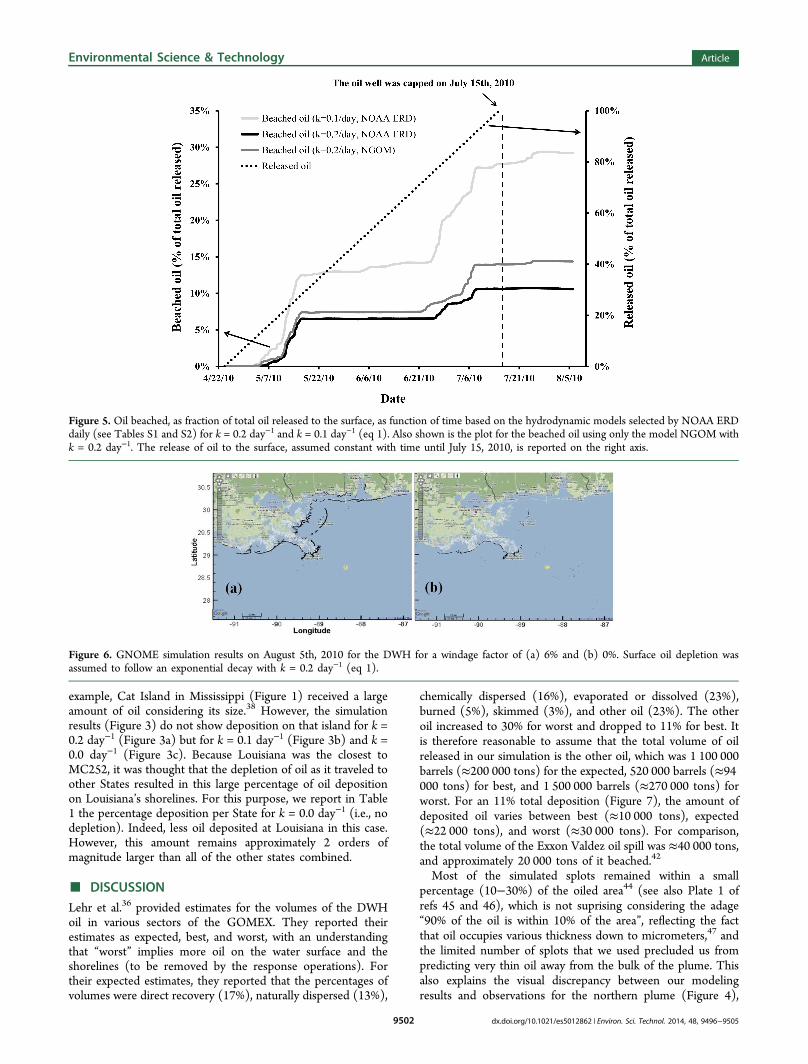
the oil that reached the shorelines (right axis) as a function oftime for the case where k = 0.2 day−1. Approximately 10% ofthe oil released reached the shorelines and beached there.Figure 5 also shows a high rate of beaching around May 10th,which was due to the deposition of oil on the ChandeleurBarrier Islands and the marshes of Louisiana (panels a, b, and cof Figure 4) and, subsequently, on the shorelines of Alabamaand Texas (in this order). The plateau in Figure 5 reflects thatlittle beaching occurred until June 26th−30th, the dates ofHurricane Alex (panels e, f, and g of Figure 4).

Figure 5 also reports the oil deposition on the shorelines fork = 0.1 day−1. One could note that the trend was the same asfor k = 0.2 day−1, but the amount of oil deposition was almosttriple that resulting from k = 0.2 day−1 (i.e., 30% of the oilreleased to the surface above MC252 reached the shorelines).One also notes that the plateau phase for k = 0.1 day−1 is not asflat, reflecting oil beaching during these periods. For the case ofk = 0.0 day−1 (i.e., no depletion), more than 96% of the oilreached the shorelines by August 6th, 2010, which is notrealistic based on observations of other spills.

Sensitivity Analyses. Figure 5 also reports the oildeposition mass for k = 0.2 day−1 when using only the modelNational Ocean Service Gulf of Mexico (NGOM) rather thanthe daily selection of models adopted by NOAA ERD (seeTables S1 and S2 of the Supporting Information). Thedifference is relatively small in terms of the time history andtotal mass. The largest difference occurred in July, probablybecause of the usage of Texas A&M University (TAMU) byNOAA ERD on July 7th, 2010. However, the results of NGOMshow a similar spatial distribution of oil (see Figure S1 of theSupporting Information) to that obtained in Figures 3a and 1,indicating the capability of the NGOM model to predict theoverall oil deposition along the shorelines. As Figure S1 of theSupporting Information shows, the model NGOM predictedmore oil deposition behind the Chandeleur Islands inLouisiana. However, it is worth noting that the purpose ofthe NOAA ERD was to direct response efforts, and it isprobable that some hydrodynamic models provided moreaccurate information than others at a particular location. Forexample, the West Florida Shelf model (see Table S1 of theSupporting Information) is most likely more accurate thanNGOM in the west Florida region. In summary, regardless ofthe depletion rate or the hydrodynamic model, Figure 5indicates that the bulk of the oil on the water surface reachedthe shorelines in two batches: May 10th and June 30th.Le Henaff et al.18 observed that wind drift plays an important

role in the oil movement, and thus, we investigate herein theimpact of the windage factor. We select for this purpose twoextreme values of the windage factor: i.e., 0 and 6%. Figure 6shows the predicted oil distribution on August 6th, 2010. The0% windage factor resulted in a much smaller oil deposition onthe shorelines than observed (Figure 1), which reflects the factthat the water currents were southward and westward, asdiscussed in details by Le Henaff et al.18 and Paris et al.,16 andthat the northern migration of oil was due in large part to wind

Figure 3. GNOME simulation results of the DWH on August 6th, 2010 assuming a constant rate of oil release to the water surface above thewellhead from April 22nd, 2010 until capping on July 15th 2010. Surface depletion based on eq 1 is (a) k = 0.2 day−1 (i.e., 20% of the oil depletes offthe surface per day), (b) k = 0.1 day−1 (10% of the oil depletes off the surface per day), and (c) k = 0.0 day−1 (i.e., no depletion). Black dots denotethe oil splots. Note the similarity of the oiled beach results for k = 0.2 day−1 to those observed in Figure 1.

Environmental Science & Technology Article

dx.doi.org/10.1021/es5012862 | Environ. Sci. Technol. 2014, 48, 9496−95059499

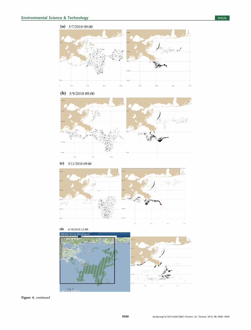
Figure 4. continued

Environmental Science & Technology Article

dx.doi.org/10.1021/es5012862 | Environ. Sci. Technol. 2014, 48, 9496−95059500

drift. The 6% windage case resulted in a higher number of oilsplots deposited along the shorelines, especially along theshoreline of Mississippi, Alabama, and Florida, which does notagree with the observation (Figure 1). This suggests that therange of 1−4% of windage factor (selected by NOAA ERD) isthe optimal range.Figure 7 provides the temporal accumulation of the beached

splots under different windage conditions. The results showthat the currents brought the oil to the shorelines on circa May10th and June 30th but that a large windage factor would haveincreased the deposition. Figure 7 is also important because itproduces the value of 30% for the oil deposition by August 6th,2010, which agrees with the simulation with k = 0.1 day−1

(Figure 5). This suggests that 30% is clearly a high upper limitfor the percentage of oil (released to the surface above MC252)reaching the shorelines, because it was obtained under extreme

modeling conditions. To put things in percepetive, thepercentage of the Exxon Valdez oil7,8 that reached the PrinceWilliam Sound (Alaska) shorelines was 50%,42 and it occurredin a cold climate where the oil source (the tanker) was relativelyclose to the shorelines. An additional comparison between thetwo spills is reported by Atlas and Hazen.43

Table 1 reports the deposition of oil on each of the fiveGOMEX U.S. States for k = 0.2 and 0.0 day−1 (no depletion).For k = 0.2 day−1, the table shows that more than 98% of the oildeposition occurred in Louisiana. The distant second wasAlabama (1.14%). The deposition at Mississippi was an orderof magnitude smaller than that at Alabama, which is due to thesheltering effects on Mississippi shorelines because of thebarrier islands of Louisiana (e.g., Chandeleur Islands).However, the model grid is relatively coarse (10 × 10 km),and a loss of precision would occur at the small scale. For

Figure 4. Comparison between (left panel) observations and (right panel) simulations at 7 dates throughout the DWH spill.

Environmental Science & Technology Article

dx.doi.org/10.1021/es5012862 | Environ. Sci. Technol. 2014, 48, 9496−95059501

example, Cat Island in Mississippi (Figure 1) received a largeamount of oil considering its size.38 However, the simulationresults (Figure 3) do not show deposition on that island for k =0.2 day−1 (Figure 3a) but for k = 0.1 day−1 (Figure 3b) and k =0.0 day−1 (Figure 3c). Because Louisiana was the closest toMC252, it was thought that the depletion of oil as it traveled toother States resulted in this large percentage of oil depositionon Louisiana’s shorelines. For this purpose, we report in Table1 the percentage deposition per State for k = 0.0 day−1 (i.e., nodepletion). Indeed, less oil deposited at Louisiana in this case.However, this amount remains approximately 2 orders ofmagnitude larger than all of the other states combined.

■ DISCUSSION

Lehr et al.36 provided estimates for the volumes of the DWHoil in various sectors of the GOMEX. They reported theirestimates as expected, best, and worst, with an understandingthat “worst” implies more oil on the water surface and theshorelines (to be removed by the response operations). Fortheir expected estimates, they reported that the percentages ofvolumes were direct recovery (17%), naturally dispersed (13%),

chemically dispersed (16%), evaporated or dissolved (23%),burned (5%), skimmed (3%), and other oil (23%). The otheroil increased to 30% for worst and dropped to 11% for best. Itis therefore reasonable to assume that the total volume of oilreleased in our simulation is the other oil, which was 1 100 000barrels (≈200 000 tons) for the expected, 520 000 barrels (≈94000 tons) for best, and 1 500 000 barrels (≈270 000 tons) forworst. For an 11% total deposition (Figure 7), the amount ofdeposited oil varies between best (≈10 000 tons), expected(≈22 000 tons), and worst (≈30 000 tons). For comparison,the total volume of the Exxon Valdez oil spill was ≈40 000 tons,and approximately 20 000 tons of it beached.42

Most of the simulated splots remained within a smallpercentage (10−30%) of the oiled area44 (see also Plate 1 ofrefs 45 and 46), which is not suprising considering the adage“90% of the oil is within 10% of the area”, reflecting the factthat oil occupies various thickness down to micrometers,47 andthe limited number of splots that we used precluded us frompredicting very thin oil away from the bulk of the plume. Thisalso explains the visual discrepancy between our modelingresults and observations for the northern plume (Figure 4),

Figure 5. Oil beached, as fraction of total oil released to the surface, as function of time based on the hydrodynamic models selected by NOAA ERDdaily (see Tables S1 and S2) for k = 0.2 day−1 and k = 0.1 day−1 (eq 1). Also shown is the plot for the beached oil using only the model NGOM withk = 0.2 day−1. The release of oil to the surface, assumed constant with time until July 15, 2010, is reported on the right axis.

Figure 6. GNOME simulation results on August 5th, 2010 for the DWH for a windage factor of (a) 6% and (b) 0%. Surface oil depletion wasassumed to follow an exponential decay with k = 0.2 day−1 (eq 1).

Environmental Science & Technology Article

dx.doi.org/10.1021/es5012862 | Environ. Sci. Technol. 2014, 48, 9496−95059502

because only a small amount of oil deposited on the easternstates. In addition, Langmuir cells, when they occur, have amajor effect on the spatial distribution of oil and its residencebelow the surface, as noted in the Braer Incident when oildisappeared for 2 days because of a storm to remerge later andreach the shorelines,48,49 and the GNOME model does notmodel explicitly the effects of Langmuir cells (and we are notaware of any oil spill model that does).It was suggested that the large extent of the oil slick might be

due to the DWH oil droplets released at depth eventuallysurfaced at locations that are far (e.g., 50 km) from the MC252well. However, we are not aware of any model that predictedsuch a behavior (see, for example, the study by Paris et al.16).However, we believe that because surface oil spills spread tovery thin thickness and that deep spills that emerge above thewell are expected to be even thinner,50 the observed spatialdistribution of oil is not due to oil upwelling after tens ofkilometers from the source.Large-scale imaging platforms, such as moderate-resolution

imaging spectroradiometer (MODIS), synthetic aperture radar(SAR), and side looking airborne radar (SLAR), providedsynoptic views of the slick, but they are unable to provide oilthickness, which was obtained using a multispectral ap-proach45,51 at select locations because the approach cannotcover areas larger than 500 km2 per flight mission. In addition,the multispectral approach was usually focused on potentialspots of thick oil to alert response vessels for interception.40

Therefore, a complete mapping of the oil thickness is notavailable. These challenges make visual observations of spilledoil a well-accepted technique.46 However, the wide range foreach color reflects the large uncertainty in evaluating thevolume of oil, as noted in the last column of Table 2, especiallyfor thicknesses less than 50 μm.

One of the commonly asked questions in the aftermath ofthe DWH was what would have been the total amount of oildeposited on the shorelines had the well been capped earlier?To evaluate the impact of earlier capping, we conductedsimulations where we assumed capping after 1, 2, 3, and 4weeks. The results of beached oil as a function of the totalreleased oil (i.e., when capped on July 15th, 2010) are reportedin Figure 8, which shows that capping the well after 1 week ofthe blowout would have resulted in shoreline deposition of only10% of the oil that was deposited when the well was cappedafter 89 days. Capping after 2 weeks would have resulted in thedeposition of 30% of oil on the shorelines. However, cappingafter 3 weeks would have been the same as capping after 4weeks (and 7 weeks; not reported herein) and would haveresulted in the deposition of 60% of the total oil depositedwhen the well was capped after 89 days. With the benefit ofhindsight, our results suggest that capping within 1 or 2 weeks

Figure 7. Percentages of total and beached oil using different windage percent for depletion following k = 0.2 day−1. The percentages of oil on theleft axis are with respect to the total (100%) released to the surface above the wellhead until capping on July 15, 2010.

Table 1. Percent Deposition of Oil Per State Based on theTotal Amount Deposited

Statek = 0.2 day−1

(Figure 3)k = 0.0 day−1, no depletion,

(Figure 5)

Louisiana 98.6 96.4Alabama 1.14 1.5Mississippi 0.09 1Florida 0.07 0.05Texas 0 1.0

Table 2. Estimation of Oil Thickness and Volume Based onIts Color, as Per the Bonn Agreement

code description/appearancelayer thickness interval

(μm) L/km2

1 sheen (silver/gray) 0.04−0.30 4−3002 rainbow 0.30−5.0 300−50003 metallic 5.0−50 5000−500004 discontinuous true oil

color50−200 50000−200000

5 continuous true oilcolor

>200 >200000

Environmental Science & Technology Article

dx.doi.org/10.1021/es5012862 | Environ. Sci. Technol. 2014, 48, 9496−95059503

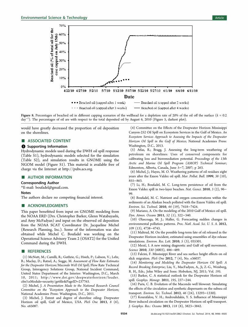
would have greatly decreased the proportion of oil depositionon the shorelines.

■ ASSOCIATED CONTENT*S Supporting InformationHydrodynamic models used during the DWH oil spill response(Table S1), hydrodynamic models selected for the simulation(Table S2), and simulation results in GNOME using theNGOM model (Figure S1). This material is available free ofcharge via the Internet at http://pubs.acs.org.

■ AUTHOR INFORMATIONCorresponding Author*E-mail: boufadel@gmail.com.NotesThe authors declare no competing financial interest.

■ ACKNOWLEDGMENTSThis paper benefitted from input on GNOME modeling fromthe NOAA ERD (Drs. Christopher Barker, Glenn Watabayashi,and Amy McFadyan) and input on the observed oil depositionfrom the NOAA SCAT Coordinator Dr. Jacqueline Michel(Research Planning, Inc.). Some of the information was alsoobtained while Michel C. Boufadel was working on theOperational Science Advisory Team 2 (OSAT2) for the UnifiedCommand during the DWH.

■ REFERENCES(1) McNutt, M.; Camilli, R.; Guthrie, G.; Hsieh, P.; Labson, V.; Lehr,B.; Maclay, D.; Ratzel, A.; Sogge, M. Assessment of Flow Rate Estimatesfor the Deepwater Horizon/Macondo Well Oil Spill; Flow Rate TechnicalGroup, Interagency Solutions Group, National Incident Command,United States Department of the Interior: Washington, D.C., March10, 2011; http://www.doi .gov/deepwaterhorizon/loader.cfm?csModule=security/getfile&PageID=237763.(2) Michel, J. A Presentation Made to the National Research CouncilCommittee on the “Ecosystem Approach to the Deepwater Horizon;National Academies Press: Washington, D.C., 2011.(3) Michel, J. Extent and degree of shoreline oiling: DeepwaterHorizon oil spill, Gulf of Mexico, USA. PloS One 2013, 8 (6),No. e65087.

(4) Committee on the Effects of the Deepwater Horizon MississippiCanyon-252 Oil Spill on Ecosystem Services in the Gulf of Mexico. AnEcosystem Services Approach to Assessing the Impacts of the DeepwaterHorizon Oil Spill in the Gulf of Mexico; National Academies Press:Washington, D.C., 2013.(5) Atlas, R.; Bragg, J. Assessing the long-term weathering ofpetroleum on shorelines: Uses of conserved components forcalibrating loss and bioremediation potential. Proceedings of the 13thArctic and Marine Oil Spill Program (AMOP) Technical Seminar;Edmonton, Alberta, Canada, June 5−7, 2007; p 263.(6) Michel, J.; Hayes, M. O. Weathering patterns of oil residues eightyears after the Exxon Valdez oil spill. Mar. Pollut. Bull. 1999, 38 (10),855−863.(7) Li, H.; Boufadel, M. C. Long-term persistence of oil from theExxon Valdez spill in two-layer beaches. Nat. Geosci. 2010, 3 (2), 96−99.(8) Boufadel, M. C. Nutrient and oxygen concentrations within thesediments of an Alaskan beach polluted with the Exxon Valdez oil spill.Environ. Sci. Technol. 2010, 44 (19), 7418−7424.(9) Mariano, A. On the modeling of the 2010 Gulf of Mexico oil spill.Dyn. Atmos. Oceans 2011, 52 (1), 322−340.(10) Olascoaga, M. J.; Haller, G. Forecasting sudden changes inenvironmental pollution patterns. Proc. Natl. Acad. Sci. U. S. A. 2012,109 (13), 4738−4743.(11) Maltrud, M. On the possible long-term fate of oil released in theDeepwater Horizon incident, estimated using ensembles of dye releasesimulations. Environ. Res. Lett. 2010, 5 (3), 035301.(12) Mezic, I. A new mixing diagnostic and Gulf oil spill movement.Science 2010, 330 (6003), 486−489.(13) Falcini, F. Mississippi River and sea surface height effects on oilslick migration. PloS One 2012, 7 (4), No. e36037.(14) Monitoring and Modeling the Deepwater Horizon Oil Spill: ARecord Breaking Enterprise; Liu, Y., MacFadyen, A., Ji, Z.-G., Weisberg,R. H., Eds.; John Wiley and Sons: Hoboken, NJ, 2011; Vol. 195.(15) Barker, C. A statistical outlook for the Deepwater Horizon oilspill. Geophys. Monogr. 2011, 195, 237−244.(16) Paris, C. B. Evolution of the Macondo well blowout: Simulatingthe effects of the circulation and synthetic dispersants on the subsea oiltransport. Environ. Sci. Technol. 2012, 46 (24), 13293−13302.(17) Kourafalou, V. H.; Androulidakis, Y. S. Influence of MississippiRiver induced circulation on the Deepwater Horizon oil spill transport.J. Geophys. Res.: Oceans 2013, 118 (8), 3823−3842.

Figure 8. Percentages of beached oil in different capping scenarios of the wellhead for a depletion rate of 20% of the oil off the surface (k = 0.2day−1). The percentages of oil are with respect to the total deposited oil by August 6, 2010 (Figure 5, darkest plot).

Environmental Science & Technology Article

dx.doi.org/10.1021/es5012862 | Environ. Sci. Technol. 2014, 48, 9496−95059504

(18) Le Henaff, M. Surface evolution of the Deepwater Horizon oilspill patch: Combined effects of circulation and wind-induced drift.Environ. Sci. Technol. 2012, 46 (13), 7267−7273.(19) Aman, Z. M.; Paris, C. B. Response to Comment on “Evolutionof the Macondo well blowout: Simulating the effects of the circulationand synthetic dispersants on the subsea oil transport. Environ. Sci.Technol. 2013, 47 (20), 11906−11907.(20) National Commission on the BP Deepwater Horizon Oil Spilland Offshore Drilling. The Gulf Oil Disaster and the Future of OffshoreDrilling; U.S. Government Printing Office: Washington, D.C., Jan2011.(21) Ryerson, T. B. Chemical data quantify Deepwater Horizonhydrocarbon flow rate and environmental distribution. Proc. Natl.Acad. Sci. U. S. A. 2012, 109 (50), 20246−20253.(22) Kujawinski, E. B. Fate of dispersants associated with theDeepwater Horizon oil spill. Environ. Sci. Technol. 2011, 45 (4), 1298−1306.(23) Hazen, T. C. Deep-sea oil plume enriches indigenous oil-degrading bacteria. Science 2010, 330 (6001), 204−208.(24) Geng, X. Mathematical modeling of the biodegradation ofresidual hydrocarbon in a variably-saturated sand column. Biode-gradation 2013, 24 (2), 153−163.(25) Elliot, A. J. Shear diffusion and the spreading of oil slicks. Mar.Pollut. Bull. 1986, 17 (7), 308−313.(26) Boufadel, M. C. The movement of oil under non-breakingwaves. Mar. Pollut. Bull. 2006, 52, 1056−1065.(27) Boufadel, M. C. Lagrangian simulation of oil droplets transportdue to regular waves. Environ. Modell. Software 2007, 22 (7), 978−986.(28) ASCE Task Committee. State-of-the-art review of modelingtransport and fate of oil spills. J. Hydraul. Eng. 1996, 122 (11), 594−609.(29) MacFadyen, A. Tactical modeling of surface oil transport duringthe Deepwater Horizon spill response. In Monitoring and Modeling theDeepwater Horizon Oil Spill: A Record Breaking Enterprise; Liu, Y.,MacFadyen, A., Ji, Z.-G., Weisberg, R. H., Eds.; John Wiley and Sons:Hoboken, NJ, 2011; pp 167−178.(30) Ippen, A. Tidal dynamics in estuaries. Part I: Estuaries ofrectangular section. In Estuary and Coastline Hydrodynamics; Ippen, A.,Ed.; McGraw-Hill: New York, 1966.(31) Committee on Oil in the Sea: Inputs, Fates, and Effects. Oil inthe Sea III: Inputs, Fates, and Effects; National Academies Press:Washington, D.C., 2003.(32) Lehr, W. Revisions of the ADIOS oil spill model. Environ.Modell. Software 2002, 17 (2), 189−197.(33) Leibovich, S. The form and dynamics of Langmuir circulations.Annu. Rev. Fluid Mech. 1983, 15 (1), 391−427.(34) Zedel, L.; Farmer, D. Organized structures in subsurface bubbleclouds: Langmuir circulation in the open ocean. J. Geophys. Res.:Oceans 1991, 96 (C5), 8889−8900.(35) Zhao, L. VDROP: A comprehensive model for dropletformation of oils and gases in liquidsIncorporation of the interfacialtension and droplet viscosity. Chem. Eng. J. 2014, 253, 93−106.(36) Lehr, B.; Bristol, S.; Possolo, A. Oil Budget Calculator: DeepwaterHorizon; Federal Interagency Solutions Group: Washington, D.C.,2010.(37) Fingas, M. An overview of in-situ burning. In Oil Spill Scienceand Technology: Prevention, Response, and Cleanup; Fingas, M., Ed.;Elsevier: Amsterdam, Netherlands, 2011; pp 737−903.(38) Operational Science Advisory Team (OSAT) Summary Reportfor Fate and Effects of Remnant Oil in the Beach Environment; OSAT:New Orleans, LA, 2011.(39) McFarlin, K. M.; Perkins, R. A.; Gardiner, W. W.; Word, J. D.Evaluating the biodegradability and effects of dispersed oil using Arctictest species and conditions: Phase 2 activities. Proceedings of the 34thArctic and Marine Oilspill Program (AMOP) Technical Seminar onEnvironmental Contamination and Response; Banff, Alberta, Canada,Oct 4−6, 2011.(40) Streett, D. D. NOAA’s satellite monitoring of marine oil. InMonitoring and Modeling the Deepwater Horizon Oil Spill: A Record

Breaking Enterprise; Liu, Y., MacFadyen, A., Ji, Z.-G., Weisberg, R. H.,Eds.; John Wiley and Sons: Hoboken, NJ, 2011; pp 9− 18.(41) Environmental Response Management Application. Web applica-tion. ERMA Deepwater Gulf Response. National Oceanic andAtmospheric Administration, 2014; http://response.restoration.noaa.gov/erma/.(42) Wolfe, D. A.; Hameedi, M. J.; Galt, J. A.; Watabayashi, G.; Short,J.; O’Claire, C.; Rice, S.; Michel, J.; Payne, J. R.; Braddock, J.; Hanna,S.; Sale, D. The fate of the oil spilled from the Exxon Valdez. Environ.Sci. Technol. 1994, 28, 560A−568A.(43) Atlas, R. M.; Hazen, T. C. Oil biodegradation andbioremediation: A tale of the two worst spills in U.S. history. Environ.Sci. Technol. 2011, 45 (16), 6709−6715.(44) Lehr, W. J. A new technique to estimate initial spill size using amodified Fay-type spreading formula. Mar. Pollut. Bull. 1984, 326−329.(45) Svejkovsky, J. Operational utilization of aerial multispectralremote sensing during oil spill response: Lessons learned during theDeepwater Horizon (MC-252) Spill. Photogramm. Eng. Remote Sens.2012, 78 (10), 1089−1102.(46) Bonn Agreement. Bonn Agreement Aerial Operations Handbook;Bonn Agreement: London, U.K., 2009.(47) National Research Council (NRC). Oil in the Sea: Inputs, Fates,and Effects; National Academies Press: Washington, D.C., 1985.(48) Pearce, F. Dispersed oil comes back to haunt Shetland. New Sci.1993, 23, 5−14.(49) Farmer, D. M.; Li, M. Oil dispersion by turbulence and coherentcirculations. Ocean Eng. 1994, 21 (6), 575−586.(50) McAuliffe, C. D. Organism exposure to volatile/solublehydrocarbons from crude oil spillsA field and laboratorycomparison. Int. Oil Spill Conf. Proc. 1987, 1987, 275−288.(51) Svejkovsky, J.; Muskat, J. Development of a Portable MultispectralAerial Sensor for Real-Time Oil Spill Thickness Mapping in Coastal andOffshore Waters; Minerals Management Service (MMS), U.S. Depart-ment of the Interior, Washington, D.C., 2009; Contract M07PC13205.

■ NOTE ADDED AFTER ISSUE PUBLICATIONThis article published August 5, 2014 with a missing reference.Reference 41 was added, the remaining references and theirrespective citations renumbered, and the revised versionpublished on August 26, 2014.

Environmental Science & Technology Article

dx.doi.org/10.1021/es5012862 | Environ. Sci. Technol. 2014, 48, 9496−95059505