\

X-525-67-495 PRE PR I NT

SIMULATION STUDY OF A PRECISE HYBRID SERVO

CONTROL SYSTEM

GEORGE C. WINSTON WILLIAM H. LONG

GPO PRICE s CFSTl PRICE(S) $

Hard copy (HC) a/ fl SEPTEMBER 1967 Microfiche (M F) / k 3’ ~

ff 653 July 85

GODDARD SPACE FLIGHT CENTER

I I (ACCESSION NUMBER) (THRU)

https://ntrs.nasa.gov/search.jsp?R=19680004338 2018-09-08T02:11:03+00:00Z

I X- 5 2 5 - 6 7 -4 95

SIMULATION STUDY OF A PRECISE HYBRID

SERVO CONTROL SYSTEM

George C . Winston

and

William H. Long

September 1967

GODDARD SPACE FLIGHT CENTER Greenbelt, Maryland

PRECEDING PAGE BLANK NOT FILMED.

SIMULATION STUDY OF A PRECISE HYBRID

SERVO CONTROL SYSTEM

George C. Winston and

William H. Long

SUMMARY

This report describes an analog computer simulation study of a precise hybrid (digital-analog) servo control system designed to control an experimen- tal optical tracking mount. The control concept developed for this system was relatively unique at the time of its inception (March 1963) and no references to performance of similar systems were lmown. As a consequence a detailed simulation study w a s performed. This study indicated the soundness of the con- cept (since confirmed experimentally) and demonstrated a tracking capability well within the two a rc second specification. Techniques were developed and demonstrated in the simulated system for overcoming nonlinear effects of am- plifier saturation and coloumb friction.

iii

TABLE OF CONTENTS

Page

INTRODUCTION .................................................. 1

SYSTEM DESCRIPTION ........................................... 1

SYSTEM ANALYSIS. .............................................. 4

ANALOG COMPUTER SIMULATION. ............................... 9

COMPUTER SIMULATION RESULTS. .............................. 15

CONCLUSION .................................................... 18

REFERENCES.. .................................................. 18

V

I

LIST OF FIGURES

Figure Page

1 Block Diagram of Control System (One Axis) ................. 3

2 Diagram for Digital Transfer Function Derivation ............ 5

3 Bode Plot 7

4 Simplified Block Diagram ..................................

................................................

8

5

6

7

8

9

10

11

Analog Computer Simulation ............................... 10

Nonlinear Model Feedback ................................. 12

Model Reference .......................................... 13

Effect of Model Reference on Limit Cycle ................... 14

Effect of Model Reference on Noise Summed into Tachometer Loop ..................................... 14

System Transient Response ................................ 16

System Tracking Error .................................... 17

vi

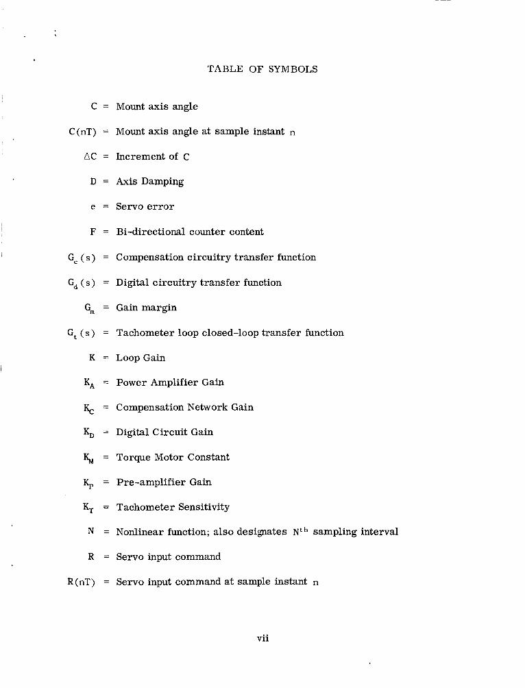
TABLE OF SYMBOLS

C = Mount axis angle

C (nT) = Mount axis angle at sample instant n

AC = Increment of C

D = Axis Damping

e = Servo e r r o r

F = Bi-directional counter content

Gc ( S ) = Compensation circuitry transfer function

Cd ( s ) = Digital circuitry transfer function

Gm = Gain margin

G, ( s ) = Tachometer loop closed-loop transfer function

K = LoopGain

K, = Power Amplifier Gain

K, = Compensation Network Gain

K, = Digital Circuit Gain

$ = Torque Motor Constant

Kp = Pre-amplifier Gain

K, = Tachometer Sensitivity

N = Nonlinear function; also designates N t h sampling interval

R = Servo input command

R (nT) = Servo input command at sample instant n

vii

TABLE OF SYMBOLS (Cont.)

s = Laplace operator

T = Samplingperiod

E = Mount motion required during the next sample period

E' = Pulse frequency corresponding to E

T~ = Compensation Time Constant

72 = Compensation Time Constant

T~ = Motor Electrical Time Constant

T,,, = Mount Mechanical Time Constant

+m = Phase Margin

viii

,

I .

SIMULATION STUDY O F A PRECISE HYBRID SERVO

CONTROL SYSTEM

INTRODUCTION

This report describes an analog computer simulation study of a precise hybrid (digital-analog) servo control system designed to position an experimen- tal optical tracking mount. The study was undertaken to determine the feasi- bility of a particular system concept and feasibility having been established to determine optimum parameter values.

The tracking mount employs an x-y axis configuration and supports a tele- scope tube having approximate dimensions of 14 feet in length and 3 feet in diameter and weighing approximately 3500 pounds. The telescope is flexible in design permitting the use of a variety of optical systems. The mount is to be used in support of various optical experiments, many employing laser optics having very narrow beamwidths. A s a result performance requirements for the control system are severe. Briefly stated these are to provide dynamic pointing accuracies to within the apparent line-of-sight jitter produced by the atmosphere; i.e., to within one to two arc seconds, at axis velocities ranging from less than sidereal rate (15 a r c seconds per sidereal second) to 3 degrees per second, and at accelerations ranging from zero to 0.15 degrees per second squared. Maxi- mum velocity should be 5 degrees per second and maximum acceleration 2 de- grees per second squared. An additional specification is for long term stability to permit extended time-exposure photography. The requirement is for an ac- cumulated drift from a tracked object (a star or deep space probe moving at essentially sidereal rate) of less than 5 a r c seconds over a tracking period of one hour. This specification requires the establishment and maintenance of an axis ra te to within one part in

SYSTEM DESCRIPTION

The resolution, repeatability and low drift rates required led to a considera- tion of digital techniques for this application. As a consequence a system con- cept based upon frequency modulation of a pulse train as the information media was developed. The pulse frequency modulation (PFM) technique has the ad- vantage of permitting control information to be processed by relatively simple, discrete digital circuitry. In this system the digital circuits perform a portion of the system compensation including one integration. The presence of this in- tegration in the driftless digital circuits eliminates all significant effects of long

1

term drifts in the following analog compensation circuitry. A further advantage of the P F M technique is that since a pulse is generated for every detectable (quantum) change in the data value the system is equivalent to a sampled data system having an infinite sampling rate. The infinite equivalent sampling rate eliminates problems inherent to conventional sampled data systems wherein a finite sampling rate introduces phase, lag and frequency folding, resulting in degradations in system stability and accuracy.

The control system provides a high degree of flexibility in using the mount by means of several operating modes. These modes include programmed drive from data stored on a punched paper tape, fixed rate sidereal drive, manual control of position and velocity and combinations of all of these. Details of the system configuration a re unique to each mode, of course, but all are based upon the block diagram of Figure 1. This is the configuration of the program mode and encompasses all of the accuracy and stability problems which require simu- lation study. The other modes differ primarily in the manner in which command data is derived.

Referring to Figure 1, it is seen that there are three loops, the inner one being an analog velocity loop closed by means of a high quality dc tachometer. The primary purposes of this loop are to linearize the motor and bearing char- acteristics and to reduce the apparent mechanical time constant.

The control system employs an encoder which has both an absolute angle output, C (NT), and an incremental output, AC, in the form of a pulse for each quantum (0.001") of shaft rotation. Physically these pulses appear on one of two lines depending upon the direction of rotation. The second loop is closed by the encoder's pulse output. This is an incremental position loop which moves the mount one encoder quantum of rotation for each pulse of the command pulse train E ' . The command pulses are also distinguished as to direction of rotation and are counted by the bi-directional counter. The instantaneous number in the counter is converted to an analog voltage which drives the mount after compen- sation. Rotation of the mount axis results in encoder incremental pulses which are applied to the counter in the sense to oppose the command pulses. When the mount has moved through the required angle the counter content is zero. By applying a continuous command pulse train to the incremental loop the mount may be made to turn at a constant desired rate.

The outer loop is closed by the absolute angle encoder output C (NT). This angle feedback is sampled once per second. The input to the loop consists of discrete time command angles which may, for example, be predictions of a spacecraft's position at specific times. These angles are also read at a rate of once per second, but in this case one sample period ahead of real time, and are designated R [ ( N + 1) T 1 .

2

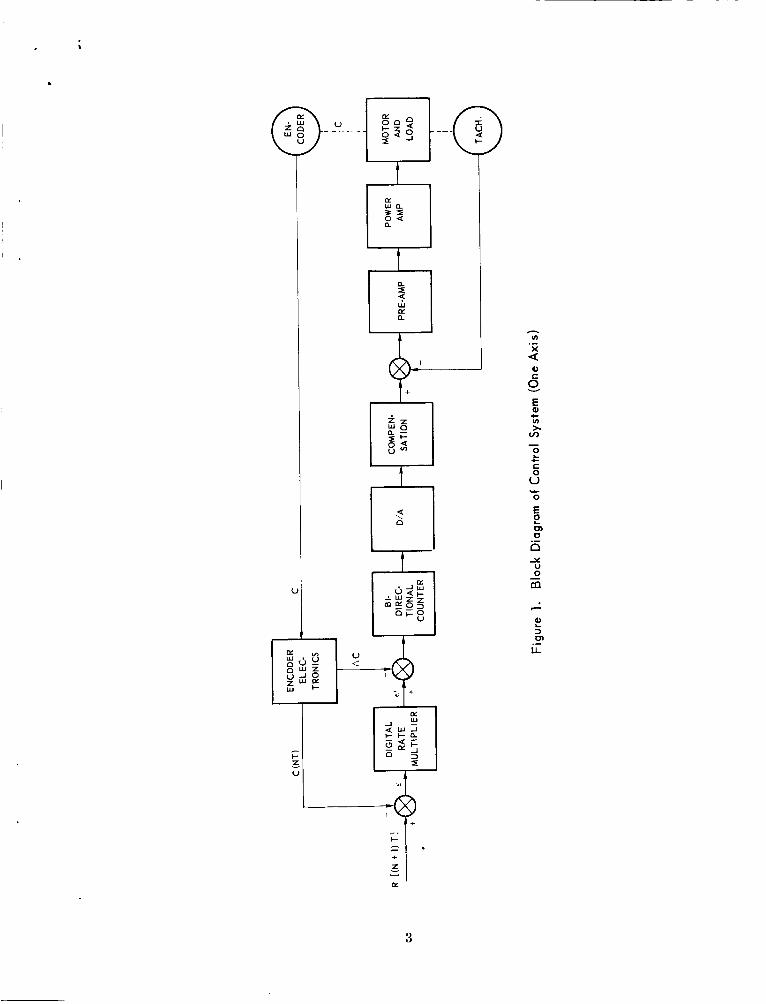
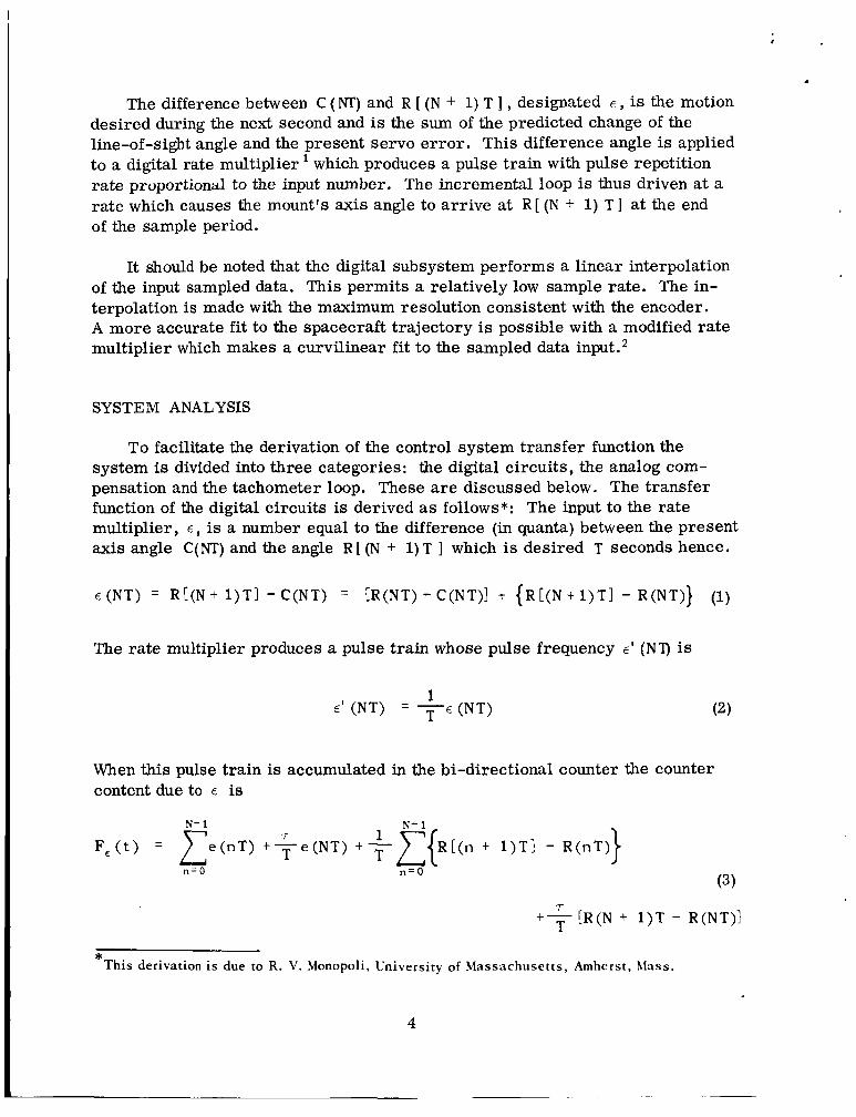
The difference between C (NI') and R [ (N + 1) T ] , designated E , is the motion desired during the next second and is the sum of the predicted change of the line-of-sight angle and the present servo error . This difference angle is applied to a digital rate multiplier which produces a pulse train with pulse repetition rate proportional to the input number. The incremental loop is thus driven at a rate which causes the mount's axis angle to arrive at R [ (N + 1) T ] at the end of the sample period.

It should be noted that the digital subsystem performs a linear interpolation of the input sampled data. This permits a relatively low sample rate. The in- terpolation is made with the maximum resolution consistent with the encoder. A more accurate fit to the spacecraft trajectory is possible with a modified rate multiplier which makes a curvilinear f i t to the sampled data input.2

SYSTEM ANALYSIS

To facilitate the derivation of the control system transfer function the system is divided into three categories: the digital circuits, the analog com- pensation and the tachometer loop. These a re discussed below. The transfer function of the digital circuits is derived a s follows*: The input to the rate multiplier, E , is a number equal to the difference (in quanta) between the present axis angle C(NT) and the angle R [ (N + 1) T ] which is desired T seconds hence.

E ( N T ) = R [ ( N + 1 ) T l - C ( N T ) [ R ( N T ) - C ( N T ) ] f { R [ ( N + l ) T ] - R ( N T ) ) (1)

The rate multiplier produces a pulse train whose pulse frequency E' (N?) is

1 E ' (NT) = T E (NT) (2 )

When this pulse train is accumulated in the bi-directional counter the counter content due to E is

(3 )

+7 [R(N + l ) T - R ( N T ) l T *

T h i s derivation is due to R. V. Monopoli , Univers i ty of M a s s a c h u s e t t s , Amherst, hlnss.

4

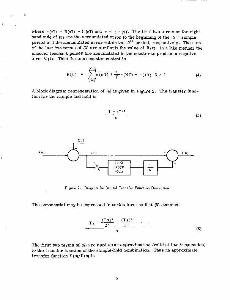
where e (nT) = R(nT) - C (nT) and T = t - NT. The first two terms on the right hand side of (3) a r e the accumulated error to the beginning of the N t h sample period and the accumulated e r ror within the Nth period, respectively. The sum of the last two terms of (3) are similarly the value of R (t). In a l.ike manner the encoder feedback pulses are accumulated in the counter to produce a negative term C ( t ) . Thus the total counter content is

r F ( t ) = r e ( n T ) + T e ( N T ) + e ( t ) ; N , 1 (4)

n = O

A block diagram representation of (4) is given in Figure 2. The transfer func- tion for the sample and hold is

R (t) -

S

Figure 2. Diagram for Digital Transfer Function Derivation

The exponential may be expressed in series form so that (5) becomes

(Ts)' ( T s ) ~ + - - . . . 3 ! T s - - 2 !

S

The first two terms of (6) a re used as an approximation (valid at low frequencies) to the transfer function of the sample-hold combination. Thus an approximate transfer function F (s)/E (s) is

5

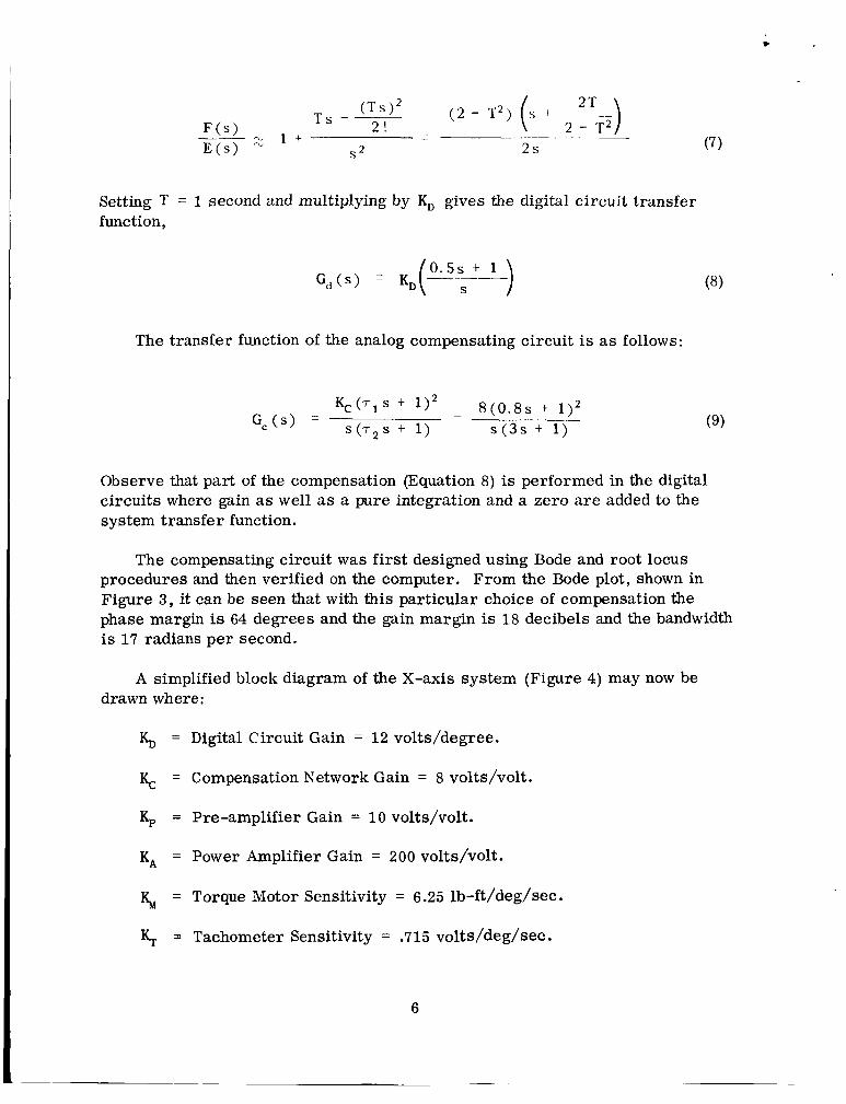
Setting T = 1 second and multiplying by K, gives the digital circuit transfer function,

The transfer function of the analog compensating circuit is as follows:

K c ( ~ l ~ -t 1 ) 2 8 ( 0 . 8 s + 1)* (9)

- -

c c ( s ) = S ( T 2 S t 1) s ( 3 s + 1)

Observe that part of the compensation (Equation 8) is performed in the digital circuits where gain a s well as a pure integration and a zero are added to the system transfer function.

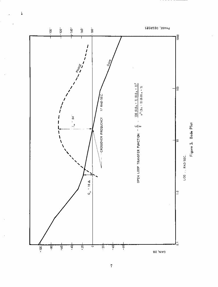
The compensating circuit w a s first designed using Bode and root locus procedures and then verified on the computer. From the Bode plot, shown in Figure 3, it can be seen that with this particular choice of compensation the phase margin is 64 degrees and the gain margin is 1 8 decibels and the bandwidth is 17 radians per second.

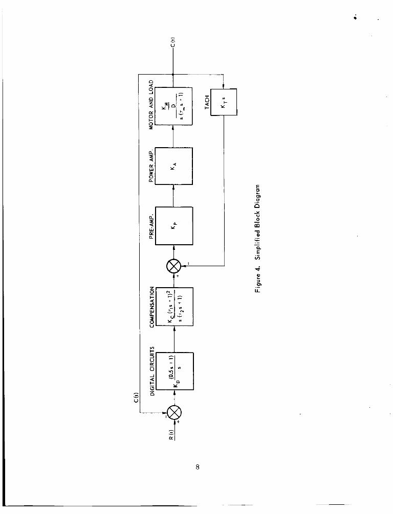
A simplified block diagram of the X-axis system (Figure 4) may now be drawn where:

K, = Digital Circuit Gain = 12 volts/degree.

K, = Compensation Network Gain = 8 volts/volt.

K, = Pre-amplifier Gain = 10 volts/volt.

K, = Power Amplifier Gain = 200 volts/volt.

$ = Torque Motor Sensitivity = 6.25 lb-ft/deg/sec.

KT = Tachometer Sensitivity = .715 volts/deg/sec.

6

0 0 0 0 0

~ C Y Z ' o

I I I /

S33t1330 '3SVHd

I

UI w I1

Z

I- U Z 3 U

2

w w U v) Z 6 w I- n 0 0 -I

Z w

0 n

I I I 0 a 0 0 y ? I

0(3 'NIV3

7

I

U 4 t- I I

Y U 0 - m

Z

v, z W a

U

v - 3 Y "

8

?! a m

LL .-

D = Axis Damping = 8.95 lb-ft/deg/sec.

T~ = Motor Electrical Time Constant = 0.035 sec.

7m = Mount Mechanical Time Constant = 11.8 sec.

71 = Compensation Time Constant = 0.8 sec.

r2 = Compensation Time Constant = 3 sec.

It should be noted that T~ < < 7,,, and can be neglected.

Since the preamplifier, power amplifier and motor a re enclosed by a feed- back loop, the closed loop transfer function of this loop must be determined in order that the open loop transfer function of the system can be found. The closed loop transfer function of the tachometer loop is:

A ’ D ( 7 m ~ t 1)

For the case of a sampling rate of one per second, the open loop transfer func- tion of the system becomes:

(11)

0 . 5 s t 1 8 ( 0 . 8 s t 1)2 1.4 - - 135(0.5s t 1) (0.8s t 1)2

s 3 (3s f 1) (0.01s t 1) ‘s(’) = s ) s ( 3 s t l ) s (0.01 s t 1)

Since the position loop has three integrations, the servo is classified a s a type 3 system; therefore, the steady state e r ro r s due to position, velocity and acceleration a r e all theoretically zero.

ANALOG COMPUTER SIMULATION

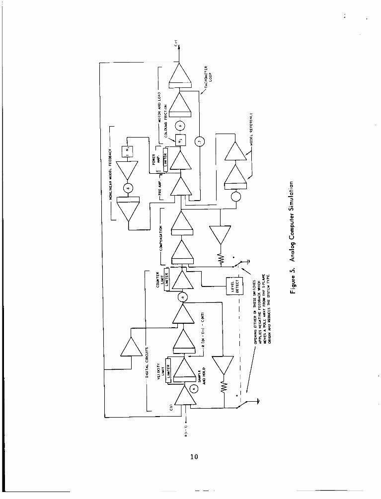
The, transfer function of the system w a s simulated on the computer as shown in Figure 5. The sample and hold function of the digital circuit w a s simulated by a motor driven switch and a hold circuit. The circuit samples the signal at point A at one second intervals and holds it for one second. Because of the wide

9

r

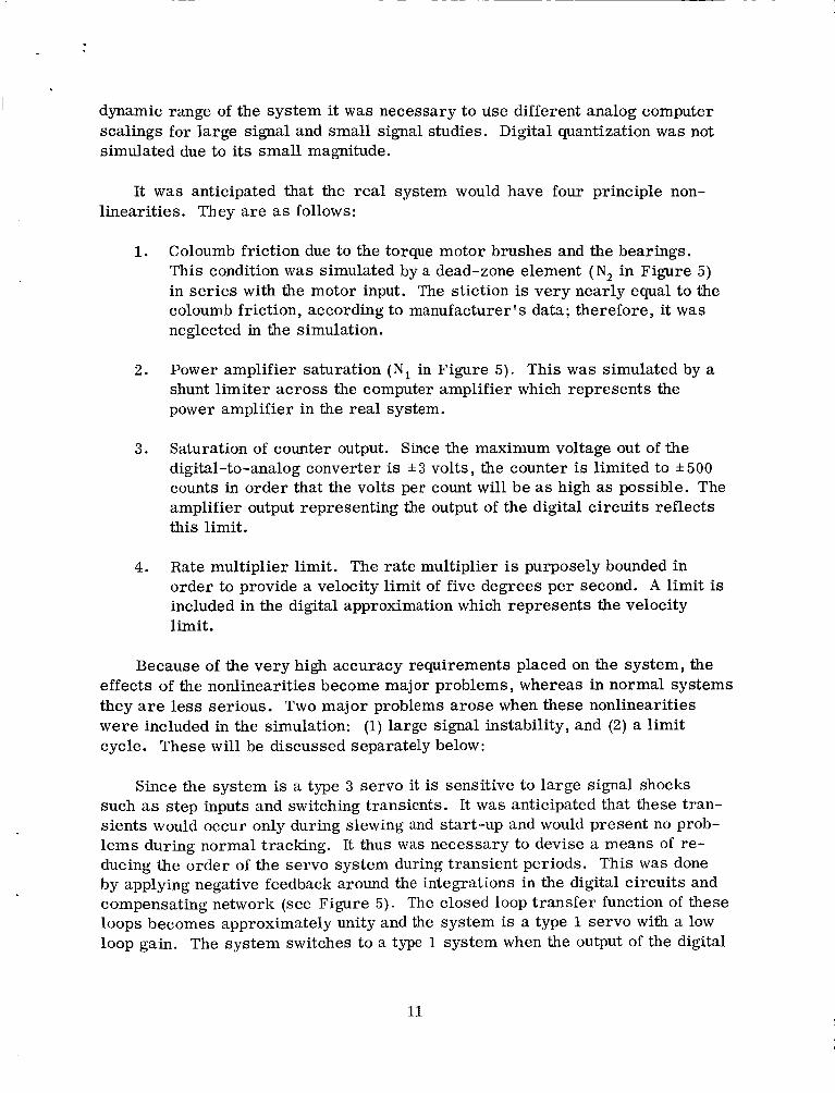
I dynamic range of the system it was necessary to U s e different analog computer scalings for large signal and small signal studies. Digital quantization w a s not simulated due to its small magnitude.

It was anticipated that the real system would have four principle non- linearities. They are as follows:

1.

2.

3 .

4.

Coloumb friction due to the torque motor brushes and the bearings. This condition w a s simulated by a dead-zone element (N, in Figure 5) in series with the motor input. The stiction is very nearly equal to the coloumb friction, according to manufacturer's data; therefore, it was neglected in the simulation.

Power amplifier saturation ( N , in Figure 5). This w a s simulated by a shunt limiter across the computer amplifier which represents the power amplifier in the real system.

Saturation of counter output. Since the maximum voltage out of the digital-to-analog converter is f 3 volts, the counter is limited to f 500 counts in order that the volts per count will be as high as possible. The amplifier output representing the output of the digital circuits reflects this limit.

Rate multiplier limit. The rate multiplier is purposely bounded in order to provide a velocity limit of five degrees per second. A limit is included in the digital approximation which represents the velocity limit.

Because of the very high accuracy requirements placed on the system, the effects of the nonlinearities become major problems, whereas in normal systems they are less serious. Two major problems arose when these nonlinearities were included in the simulation: (1) large signal instability, and (2) a limit cycle. These wil l be discussed separately below:

Since the system is a type 3 servo it is sensitive to large signal shocks such as step inputs and switching transients. It w a s anticipated that these tran- sients would occur only during slewing and start-up and would present no prob- lems during normal tracking. It thus was necessary to devise a means of re- ducing the order of the servo system during transient periods. This was done by applying negative feedback around the integrations in the digital circuits and compensating network (see Figure 5). The closed loop transfer function of these loops becomes approximately unity and the system is a type 1 servo with a low loop gain. The system switches to a type 1 system when the output of the digital

11

circuits nears saturation, indicating a large e r ror . When the output returns to some nominal low value the system switches to a type 3 system.

t t x - - N l

R - Go

The transient introduced when the system switches from a type 1 to a type 3 w a s large enough to cause the system to go ifito oscillations because of power amplifier saturation. A scheme w a s tried which allowed the system to switch from a type 1 to a type 2 to a type 3 in a timed sequence, but again, the tran- sients caused instability.

-

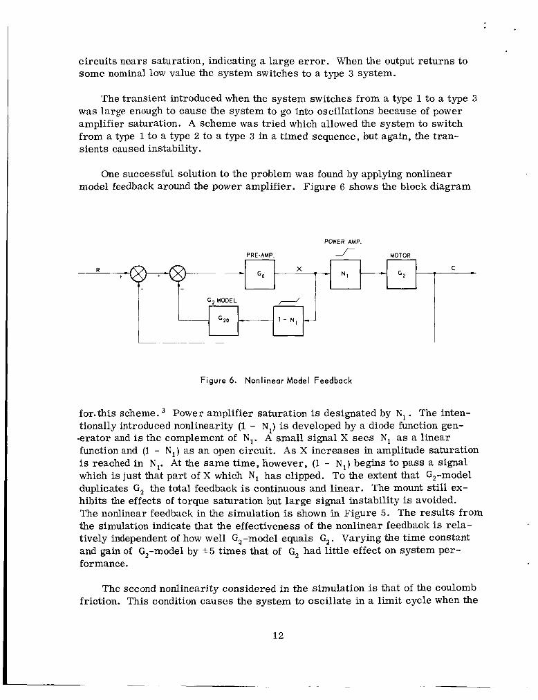
One successful solution to the problem w a s found by applying nonlinear model feedback around the power amplifier. Figure 6 shows the block diagram

G, MODEL 4

G,, -

C . -

1 - N , c

Figure 6. Nonlinear Model Feedback

for.this scheme. tionally introduced nonlinearity (1 - N1) is developed by a diode function gen- .erator and is the complement of N, . A small signal X sees N, as a linear function and (1 - N1) as an open circuit. As X increases in amplitude saturation is reached in N,. At the same time, however, (1 - N,) begins to pass a signal which is just that part of X which N, has clipped. To the extent that G,-model duplicates C, the total feedback is continuous and linear. The mount still ex- hibits the effects of torque saturation but large signal instability is avoided. The nonlinear feedback in the simulation is shown in Figure 5. The results from the simulation indicate that the effectiveness of the nonlinear feedback is rela- tively independent of how well C,-model equals C,. Varying the time constant and gain of G,-model by * 5 times that of G, had little effect on system per- formance.

Power amplifier saturation is designated by N, . The inten-

The second nonlinearity considered in the simulation is that of the coulomb friction. This condition causes the system to oscillate in a limit cycle when the

12

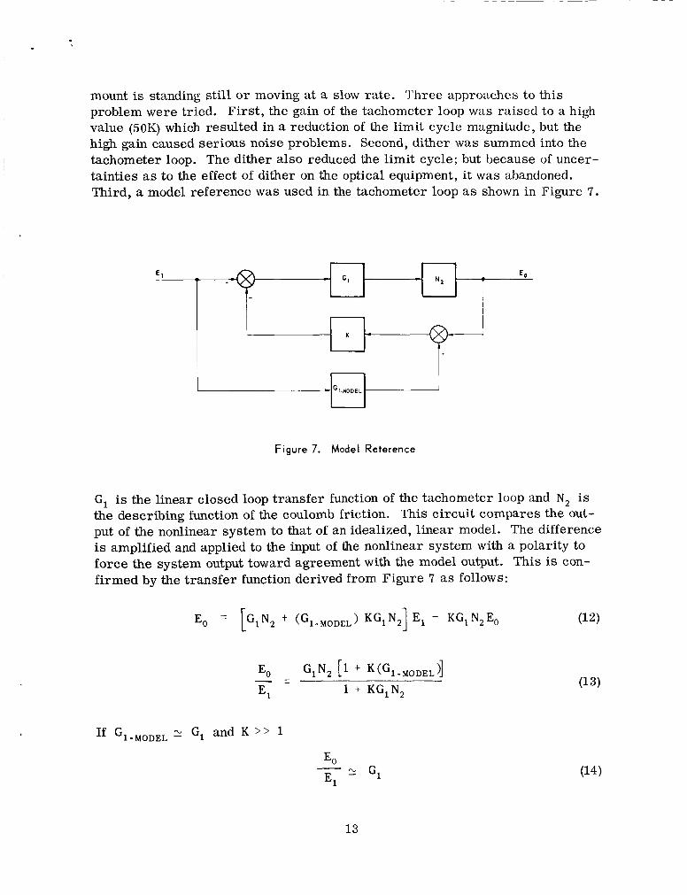
mount is standing still o r moving at a slow rate. Three approaches to this problem were tried. First, the gain of the tachometer loop was raised to a high value (50K) which resulted in a reduction of the limit cycle magnitude, but the high gain caused serious noise problems. Second, dither was summed into the tachometer loop. The dither also reduced the limit cycle; but because of uncer- tainties a s to the effect of dither on the optical equipment, it was abandoned. Third, a model reference was used in the tachometer loop a s shown in Figure 7.

Figure 7. Model Reterence

G, is the linear closed loop transfer function of the tachometer loop and N, is the describing function of the coulomb friction. ‘This circuit compares the out- put of the nonlinear system to that of an idealized, linear model. The difference is amplified and applied to the input of the nonlinear system with a polarity to force the system output toward agreement with the model output. This is con- firmed by the transfer function derived from Figure 7 as follows:

If Gl~,o,E, 2 C, and K > > 1

EO

El - 2r C,

13

3 S T C p-p

1 Sec p-p * t

I 1 1 1 -

CAL.: 0.09 Sz/rnrn t LIMIT CYCLE WITHOUT MODEL,

OUTPUT WITH INPUT = 0 ,IMIT CYCLE WITH MODEL, OUTPUT WITH INPUT = 0

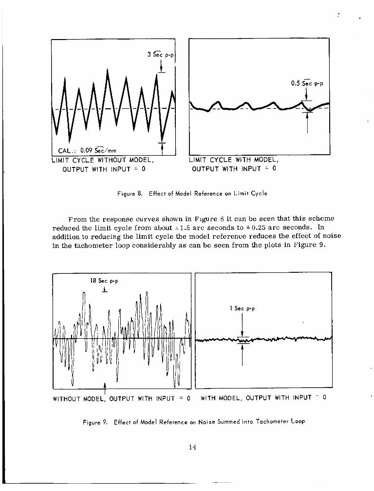
Figure 8. Effect of Model Reference on L i m i t Cycle

From the response curves shown in Figure 8 it can be seen that th i s scheme reduced the limit cycle from about f 1.5 a rc seconds to f 0.25 a r c seconds. In addition to reducing the limit cycle the model reference reduces the effect of noise in the tachometer loop considerably as can be seen from the plots in Figure 9.

I 18 Sec p-p I

I

WITHOUT MODEL, OUTPUT WITH INPUT = 0 WITH MODEL, OUTPUT WITH INPUT = 0

Figure 9. Effect of Model Reference on Noise Summed in to Tachometer LOOP

14

I

Again, the simulation indicated that the effectiveness of the model is relatively independent of how wel l the model of G, equals the true G, over a range of agreement that should be readily achieved in practice.

COMPUTER SIMULATION RESULTS

With the computer implemented as shown in Figure 5, various tests were conducted to determine if the control system could meet the specifications. Some of these tests are described below.

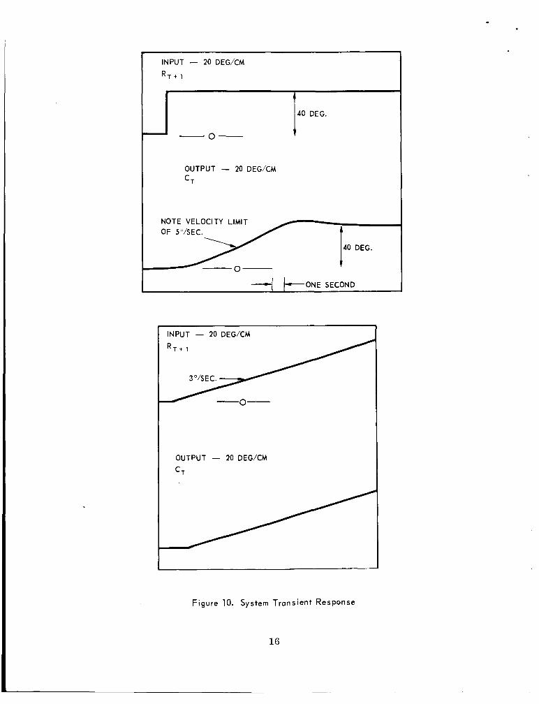
The system response to a step of position and velocity is shown in Figure 10. Note that the output response lags the position command by one second, verifying that the position command is truly R [ ( N + 1) t ] .

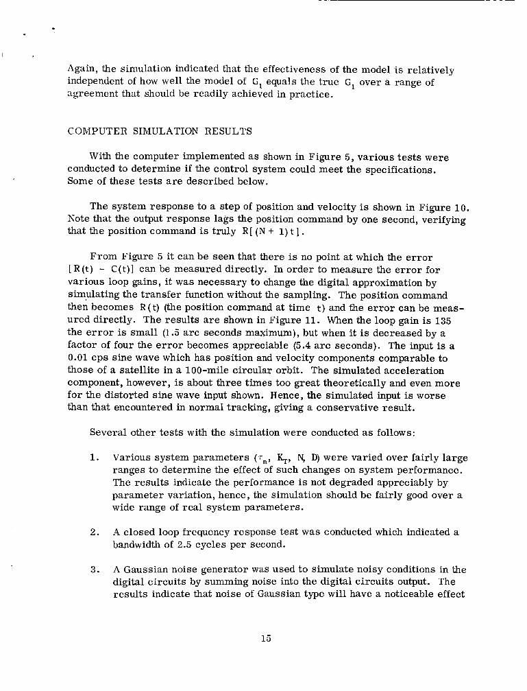
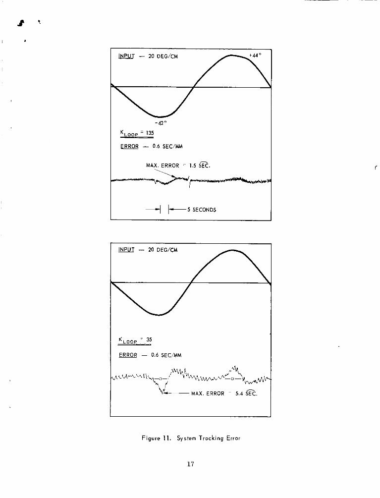
From Figure 5 it can be seen that there is no point at which the e r r o r [ R (t) - C ( t ) ] can be measured directly. In order to measure the e r ro r for various loop gains, it w a s necessary to change the digital approximation by simulating the transfer function without the sampling. The position command then becomes R (t) (the position command at time t ) and the e r r o r can be meas- ured directly. The results are shown in Figure 11. When the loop gain is 135 the e r r o r is small (1.5 a r c seconds maximum), but when it is decreased by a factor of four the e r r o r becomes appreciable (5.4 arc seconds). The input is a 0.01 cps sine wave which has position and velocity components comparable to those of a satellite in a 100-mile circular orbit. The simulated acceleration component, however, is about three times too great theoretically and even more for the distorted sine wave input shown. Hence, the simulated input is worse than that encountered in normal tracking, giving a conservative result.

Several other tests with the simulation were conducted as follows:

1.

2.

3 .

Various system parameters ( T ~ , q, N, D) were varied over fairly large ranges to determine the effect of such changes on system performance. The results indicate the performance is not degraded appreciably by parameter variation, hence, the simulation should be fairly good over a wide range of real system parameters.

A closed loop frequency response test w a s conducted which indicated a bandwidth of 2.5 cycles per second.

A Gaussian noise generator was used to simulate noisy conditions in the digital circuits by summing noise into the digital circuits output. The results indicate that noise of Gaussian type w i l l have a noticeable effect

15

INPUT - 20 DEG/CM

R T t l

OUTPUT - 20 DEG/CM CT

NOTE VELOCITY LIMIT OF 5"/SEC.

40 DEG.

0-

-1 +ONE SECOND

INPUT - 20 DEG/CM

R T t l

OUTPUT - 20 DEG/CM

CT

Figure 10. System T r a n s i e n t R e s p o n s e

16

-42"

p_ K ~ o o p 135

ERROR - 0.6 SEC/MM

MAX. ERROR = 1.5 SFC.

k 5 SECONDS

KLOOP = 35

ERROR - 0.6 SEC/MM

vi- MAX. ERROR 5.4 SFC.

r

Figure 11. System Tracking Error

17

on the system output and that pains must be taken to develop a clean signal at this point.

4. Low frequency sine waves (.001 cycles per second) were summed into the tachometer loop to simulate amplifier drift. The frequency of these drifts is well within the servo bandwidth, therefore, the servo compen- sates for them.

CONCLUSION

Results of the simulation study indicated that the system a s designed would meet the specifications. Modeling techniques were developed which demonstrated the ability to cope with nonlinearities considerably more severe than expected in practice. Whether these techniques wi l l have to be incorporated in the final system will be determined by experimental results.

Since completion of this study the system has been built. It is undergoing thorough testing at this time. Results from these tests wil l be published in the near future.

REFERENCES

1. Digital Linear Interpolation and the Binary Rate Multiplier, W. Arnstein, H . W . Mergler and B. Singer, 'IControl Engineering", June 1964.

2. A Digital Rate Multiplier for Curvilinear Interpolation of Sampled Data, G . C. Winston, NASA Report No. X-525-67-277, June, 1967.

3. Adaptive Control Systems, E . Mishkin and L. Brann, Jr., McGraw-Hill Book Company, New York, 1961, pp. 204-207.

18