SIMULATIONS OF ACCRETION POWERED SUPERNOVAE IN …

The Astrophysical Journal, 750:163 (22pp), 2012 May 10 doi:10.1088/0004-637X/750/2/163C© 2012. The American Astronomical Society. All rights reserved. Printed in the U.S.A.

SIMULATIONS OF ACCRETION POWERED SUPERNOVAEIN THE PROGENITORS OF GAMMA-RAY BURSTS

Christopher C. Lindner1, Milos Milosavljevic, Rongfeng Shen2, and Pawan KumarDepartment of Astronomy, University of Texas, 1 University Station C1400, Austin, TX 78712, USA

Received 2011 August 5; accepted 2012 March 19; published 2012 April 26

ABSTRACT

Observational evidence suggests a link between long-duration gamma-ray bursts (LGRBs) and Type Ic supernovae.Here, we propose a potential mechanism for Type Ic supernovae in LGRB progenitors powered solely by accretionenergy. We present spherically symmetric hydrodynamic simulations of the long-term accretion of a rotatinggamma-ray burst progenitor star, a “collapsar,” onto the central compact object, which we take to be a black hole.The simulations were carried out with the adaptive mesh refinement code FLASH in one spatial dimension and withrotation, an explicit shear viscosity, and convection in the mixing length theory approximation. Once the accretionflow becomes rotationally supported outside of the black hole, an accretion shock forms and traverses the stellarenvelope. Energy is carried from the central geometrically thick accretion disk to the stellar envelope by convection.Energy losses through neutrino emission and nuclear photodisintegration are calculated but do not seem importantfollowing the rapid early drop of the accretion rate following circularization. We find that the shock velocity, energy,and unbound mass are sensitive to convective efficiency, effective viscosity, and initial stellar angular momentum.Our simulations show that given the appropriate combinations of stellar and physical parameters, explosions withenergies ∼5 × 1050 erg, velocities ∼3000 km s−1, and unbound material masses �6 M� are possible in a rapidlyrotating 16 M� main-sequence progenitor star. Further work is needed to constrain the values of these parameters,to identify the likely outcomes in more plausible and massive LRGB progenitors, and to explore nucleosyntheticimplications.

Key words: accretion, accretion disks – black hole physics – gamma-ray burst: general – stars: winds, outflows –supernovae: general

Online-only material: color figures

1. INTRODUCTION

A clear observational link has been established between long-duration gamma-ray bursts (LGRBs) and Type Ic supernovae(Galama et al. 1998, 2000; Reichart 1999; Bloom et al. 2002;Della Valle et al. 2003, 2006; Garnavich et al. 2003; Hjorthet al. 2003; Kawabata et al. 2003; Stanek et al. 2003; Mathesonet al. 2003; Malesani et al. 2004; Campana et al. 2006;Mirabal et al. 2006; Modjaz et al. 2006; Pian et al. 2006;Chornock et al. 2010; Cobb et al. 2010; Starling et al. 2011).However, only a small percentage of Type Ic supernovaeexhibit the late-time radio signatures of LGRBs (Podsiadlowskiet al. 2004; Soderberg et al. 2006). LGRBs are believed to bemanifestations of rotationally powered ultrarelativistic outflowsdeveloping in the wake of the formation of black holes or neutronstars in rotating progenitor. However, the exact mechanismfor the production of LGRBs and their associated supernovaeremains a subject of debate (Woosley & Bloom 2006; Hjorth &Bloom 2011, and references therein). At present, it is not clearwhether the processes that give rise to LGRBs also drive stellarexplosions, or whether the explosions are driven independently,perhaps by the standard, neutrino-mediated mechanism.

In the standard supernova mechanism, an outward-movingshock forms after core-bounce. This shock stalls, but maybe reinvigorated by heating by neutrinos emitted during theneutronization near the proto-neutron star (Bethe & Wilson1985), and in principle drive the star to explosion in the so-called

1 NSF Graduate Research Fellow.2 Department of Astronomy, & Astrophysics, University of Toronto, 50 St.George St., Toronto, Ontario M5S 3H4, Canada.

delayed neutrino mechanism. Some simulations of this processin at least two spatial dimensions seem to produce successfulexplosions (see, e.g., Buras et al. 2006b; Scheck et al. 2006;Mezzacappa et al. 2007; Murphy & Burrows 2008; Marek &Janka 2009; Nordhaus et al. 2010), although the success of two-dimensional and possibly three-dimensional simulations maybe dependent upon the progenitor mass and the treatment ofneutrinos (Buras et al. 2006a; Nordhaus et al. 2010). Supernovaeassociated with LGRBs seem to be more energetic than thetypical Type Ic supernovae (Iwamoto et al. 1998; Woosley &MacFadyen 1999; Mazzali et al. 2003, 2006), with large kineticenergies reaching ∼1052 erg. Even if the neutrino mechanismcan unbind the star, it still seems unclear whether it can deliverthe energies found in supernovae associated with LGRBs.An alternative or augmentative explosion mechanism may berequired to explain the supernovae associated with LGRBs.Alternatives to the neutrino mechanism call on the extraction ofthe rotational energy of the central compact object—a neutronstar or a black hole—or on tapping the gravitational energy ofthe material accreting toward the compact object. It remains tobe determined which, if any, of the alternative pathways candeliver the large energies, and what are the resulting compactremnant masses.

If the post-bounce neutrino-mediated energy transfer is tooweak to unbind all of the infalling stellar strata, some materialmay continue to fall onto the proto-neutron star and possiblytake it to collapse further into a black hole (e.g., Burrows1986; MacFadyen et al. 2001; Heger et al. 2003; Zhang et al.2008; Sekiguchi & Shibata 2011; O’Connor & Ott 2010).This is especially relevant for rapidly rotating progenitors,as the progenitors with rapidly rotating cores may produce

1

http://dx.doi.org/10.1088/0004-637X/750/2/163

The Astrophysical Journal, 750:163 (22pp), 2012 May 10 Lindner et al.

lower neutrino luminosities, decreasing the effectiveness of theneutrino-powered explosion mechanism (Fujimoto et al. 2006;Lee & Ramirez-Ruiz 2006).

The infall or fallback of the stellar envelope should continuepast the initial emergence of the event horizon, but then thestructure of the accretion flow becomes sensitive to its angu-lar momentum content. Given sufficient angular momentum,the flow becomes rotationally supported. Such a “collapsar”configuration has been proposed to naturally lead to the ultra-relativistic outflow in LRGBs (Woosley 1993), as gamma rayscan be produced in an ultrarelativistic jet launching from themagnetosphere of the black hole that forms in the aftermath ofthe collapse of the rotating progenitor. The jet is powered by acontinuous infall and disk-like accretion of the progenitor star’sinterior.

It has long been hypothesized that a “wind” outflowing froma collapsar accretion disk could unbind the stellar envelopeand synthesize sufficient 56Ni to produce an optically brightsupernova (e.g., MacFadyen & Woosley 1999; Pruet et al. 2003,2004; Kohri et al. 2005). The dynamics of the energy flow insuch a system has yet to be elucidated. In the present study, weutilize one-dimensional hydrodynamic simulations with rotation(1.5D) to test the hypothesis that accretion power can drivean explosion of the star. We do not simulate the core bounce,and simply posit that any prompt and neutrino-reinvigoratedshock has failed and that the stellar atmosphere has not acquiredoutward motion and is free to accrete toward the black hole.

In Lindner et al. (2010), we simulated the post-core-collapse hydrodynamical evolution of the rapidly rotating14 M� Wolf–Rayet (W-R) stellar model 16TI of Woosley &Heger (2006) that has been proposed as an LGRB progenitor.The rate at which the infalling stellar envelope was being ac-creted onto the black hole evolved through two distinct phasesduring the first ∼200 s following the initial collapse of the stel-lar core. First, the low specific angular momentum material ofthe inner layers of the star accreted quasi-spherically throughthe inner boundary and is presumed to have accreted onto theblack hole. Then, the material that had sufficient angular mo-mentum to become rotationally supported on the computationalgrid formed a thick accretion torus. Simultaneously, an accre-tion shock appeared at the innermost radii and traversed the star.Most of the stellar envelope traversed by the shock was in radialhydrostatic equilibrium and convective; convection transportedthe energy dissipated at the smallest simulated radii toward theexpanding shock. The central accretion rate was nearly time-independent prior to rotating torus and shock formation, anddropped sharply afterward. The abrupt drop of the accretion rateclosely resembled the prompt γ -ray and the early X-ray LGRBlight curves measured with the NASA Swift satellite (Tagliaferriet al. 2005; Nousek et al. 2006; O’Brien et al. 2006), addingweight to the hypothesis that the light curves are responding toan evolution of the central accretion rate (Kumar et al. 2008a,2008b). Because the innermost simulated radius was 500 km,much larger than the innermost stable circular orbit around thecentral black hole (5–50 km), the accreted-mass-to-energy con-version efficiency was low and the shock acquired relatively lowvelocities, ∼1000 km s−1, while in the interior of the star. Thestar did not explode, but only lost mass to the thermally drivenwind that set in after the shock had traversed the star.

In collapsars, a substantially larger accretion energy is dis-sipated at the radii left out from the Lindner et al. (2010)simulations, closer to the black hole, but only a fraction ofthis energy couples to the stellar envelope. The rest may be

lost to the emission of neutrinos and to the photodisintegra-tion of hydrostatic elements into free nucleons as well as toadvection into the black hole. Crude analytical considerations(Milosavljevic et al. 2012) suggest that following shock for-mation and the rapid accretion rate drop seen in Lindner et al.(2010), neutrino losses are relatively small. Then, the amountof energy transferred onto the envelope is determined by thecompetition of the inward advective and the outward convectiveenergy transport. The advection arises from the inward drift ofthe fluid in response to magnetohydrodynamic (MHD) stresses;the convection arises from entropy gradients arising from thedissipation of MHD turbulence. If convective transport is effi-cient, the amount of energy transferred from near the black holeto the shocked envelope can be sufficient to drive a fast shockwith velocity �1000 km s−1 and unbind the star. The modelof Milosavljevic et al. (2012) suggests that the parameters de-termining the viability and energy of such accretion-poweredsupernovae are the viscous stress-to-pressure ratio α and theconvective mixing length λconv. The model could not, of course,capture the consequences of the interplay of pressure and rota-tion at the critical radii where the two sources of radial supportagainst gravity are comparable.

In this work, we show the results of a series of rotating one-dimensional simulations of the immediate aftermath of the col-lapse of a rapidly rotating LGRB progenitor star’s core. Whileone-dimensional, our simulations include rotation in a spher-ically averaged sense and implement a modified α-viscosityprescription. One customarily refers to such simulations as“1.5 dimensional.” They also take into account optically thincooling by neutrino emission, cooling and heating by nuclearprocesses, and energy and compositional transport by convec-tion in the mixing length theory approximation. This work iscomplementary to our rotating two-dimensional simulations(2.5D) of collapsar accretion (Lindner et al. 2010), in whichwe simulated only relatively large radii and did not incorpo-rate nuclear and neutrino physics. Here, we sacrifice in spatialdimensionality to make it possible to track rudimentary nu-clear compositional transformation and simulate smaller radii(r > 25 km) over similarly extended time periods (∼40–100 s).In the presence of cooling by neutrino emission the rotatingcentral torus may be geometrically thin (e.g., MacFadyen &Woosley 1999; Popham et al. 1999; Kohri et al. 2005; Chen& Beloborodov 2007; Sekiguchi & Shibata 2011; Taylor et al.2011). Therefore, we include corrections to approximate the ef-fects of such flow. The principal source of model uncertaintyis the efficiency of convection, which in the mixing length ap-proximation can be parameterized with an effective value ofthe mixing length. To our best knowledge, there has not beena systematic first principles study of convective efficiencies inthe rapidly convecting regime. Thus the mixing length λconv andthe viscous shear stress-to-pressure ratio α are the parameterdependences that we explore.

A magnetic outflow driven by a proto-neutron star may carryan energy similar to that of a supernova (e.g., Bisnovatyi-Kogan 1971; Wheeler et al. 2000; Thompson et al. 2004;Bucciantini et al. 2007; Burrows et al. 2007; Dessart et al.2008). However, the outflow may be too axially collimated toproduce a standard, quasi-spherical explosion (Bucciantini et al.2008, 2009). Here, we assume that any explosion mechanismpreceding the collapse into a black hole has failed. Clearly,our one-dimensional model cannot capture the effects of theformation of a magnetized jet, after an accretion disk has formed.Although this is an integral component to the collapsar model

2


for LGRBs, we omit any treatment of the jet in the presentwork.

This work is organized as follows. In Section 2, we discussour numerical algorithm. In Section 3, we present the results ofour simulations. In Section 4, we identify the parameters criticalto our model and discuss their implications for real accretionpowered supernovae. Finally, in Section 5, we summarize ourconclusions.

2. NUMERICAL ALGORITHM

The simulations were carried out with the piecewise-parabolicmethod (PPM) solver in the adaptive-mesh-refinement codeFLASH (Fryxell et al. 2000), version 3.2, in one spatial dimen-sion. Although the rotating stellar collapse is inherently threedimensional, we have chosen to approximate the key multidi-mensional effects, including angular momentum transport andconvective energy and compositional transport, with a spheri-cally averaged transport scheme. In Section 2.1, we describe ourimplementation of angular momentum transport. In Section 2.2,we describe our calculation of the self-gravity of the fluid. InSection 2.3, we describe our modeling of the transition towardnuclear statistical equilibrium (NSE) in the hot inner accretionflow. In Section 2.4, we discuss cooling by neutrino emission.In Section 2.5, we describe our treatment of convective energytransport and compositional mixing. In Section 2.6, we describethe corrections that we apply in situations where, in the presenceof cooling, the accretion flow is expected to be geometricallythin. In Section 2.7, we describe our initial and boundary condi-tions. In Section 2.8, we show the results from tests of the code.Finally, in Section 2.9, we briefly review the various limitationsof our method.

2.1. Angular Momentum

To include rotation and angular momentum transport inour one-dimensional model, we track the specific angularmomentum � ≡ rvφ , where vφ is the azimuthal velocity, whichwe interpret as the mass-weighted spherical average of anunderlying polar-angle-dependent angular momentum �(r, θ ).If, e.g., spherical shells rotate rigidly, �(r, θ ) ∝ sin2 θ , and thefluid density is spherically symmetric, then the one-dimensionalspecific angular momentum is two-thirds of the midplane value,� = 2/3�mid. The azimuthal Navier-Stokes equation, combinedwith the equation of mass continuity, then implies the one-dimensional angular momentum transport equation (see, e.g.,Thompson et al. 2005)

∂(ρ�)

∂t+

1

r2

∂(r2vrρ�)

∂r− 1

r2

∂

∂r(r3νρσrφ) = 0, (1)

where ν is a shear viscosity and

σrφ = r∂

∂r

(�

r2

)(2)

is the r−φ component of the shear tensor. The energy dissipatedthrough shear viscosity was accounted for by including thespecific heating rate (see, e.g., Landau & Lifshitz 1959)

εvisc ≡ Qvisc

ρ= νσ 2

rφ, (3)

where Qvisc denotes the volumetric viscous heating rate. Thedimensional reduction in Equation (1) is inaccurate in regions

where the disk is geometrically thin. There the mass-weightedspherical average closely approximates the midplane value,� ∼ �mid. We ignore this effect, but we do incorporate ther-modynamic corrections addressing the transition to a thin diskin Section 2.6.

Our treatment of shear viscosity is similar to our methodol-ogy in Lindner et al. (2010), and for completeness we reproduceour methodology here. Since we do not simulate the magneticfield of the fluid, we utilize a local definition of the shear vis-cosity to emulate the magnetic stress arising from the nonlineardevelopment of the magnetorotational instability (MRI; Balbus& Hawley 1998 and references therein). It should be kept inmind, however, that the effects of MRI are in some respectsvery different from those of the viscous stress. For example, thethick disk surrounding our collapsar black hole is convective;in unmagnetized accretion flows convection transports angu-lar momentum inward, toward the center of rotation (Ryu &Goodman 1992; Stone & Balbus 1996; Igumenshchev et al.2000), whereas in magnetized flows, convection can also trans-port angular momentum outward (Balbus & Hawley 2002;Igumenshchev 2002; Igumenshchev et al. 2003; Christodoulouet al. 2003). Although we include treatment for convective en-ergy flux and compositional mixing (see Section 2.5), we do notinclude angular momentum transport by convection.

Our definition of the local viscous stress emulating the MRImust be valid under rotationally supported, pressure supported,and freely falling conditions, and we proceed as in Lindneret al. (2010). Thompson et al. (2005) suggest that since thewavenumber of the fastest growing MRI mode, which is givenby the dispersion relation vAk ∼ Ω where vA is the Alfvenvelocity and Ω = vφ/r is the angular velocity, should be aboutthe gas pressure scale height in the saturated quasi-state state,k ∝ H−1, the Maxwell ρv2

A and viscous νρΩ stresses (up tofactors in |d ln Ω/d ln r| that we neglect) can be equated if theviscosity is given by

νMRI = αH 2Ω, (4)

where α is a dimensionless parameter. If the pressure scaleheight is defined locally,

H = |∇ ln P |−1, (5)

the viscosity defined in Equation (4) suffers from divergences atpressure extrema. To alleviate this problem, as in Lindner et al.(2010), we define a second viscosity according to the Shakura& Sunyaev (1973) prescription

νSS = αP

ρΩ−1. (6)

Shakura–Sunyaev viscosity overestimates the magnetic stress instratified hydrostatic atmospheres. We thus set the viscosity inEquations (1) and (3) to equal the harmonic mean of the abovetwo viscosities

ν = 2 νMRI νSS

νMRI + νSS, (7)

where the pressure gradient in Equation (5) is calculated by thefinite differencing of pressure in neighboring fluid cells. Ad-ditionally, we have applied a Gaussian kernel smoothing to theradial dependence of H to help filter short-wavelength numericalinstabilities. We describe this procedure in Section 2.5.

In FLASH, we treat specific angular momentum as a con-served “mass scalar” that is being advected with the fluid, which

3


makes ρ� a conserved variable; the corresponding centrifugalforce is then incorporated in the calculation of the gravitationalacceleration as we explain in Section 2.2 below. Then the thirdparabolic term in Equation (1) is computed explicitly throughthe inclusion of the radial ρ�-flux −rνρσrφ in the advectionof �.

Numerical stability of an explicit treatment of a parabolicterm places an upper limit on the time step

Δt <Δr2

2ν, (8)

where Δr is the grid resolution. For α � 0.01, the viscoustime step in our simulations becomes significantly shorter thanthe Courant time step. In our test integrations with a γ -lawequation of state (EOS; Lindner et al. 2010), we find that, whilenot implying an outright instability, a choice of Δt that saturatesthe limit in Equation (8) results in weak stationary staggeredperturbations in the fluid variables. We ignore this complicationand allow our time step to be set by the limit in Equation (8)of the cell with the smallest viscous diffusion time across thecell.

2.2. Gravity

We calculate contributions to the gravitational potential froma central point mass and a spherically symmetric extendedenvelope. General relativistic effects become important at theinnermost radius, which in some simulations is as small asrmin = 25 km. At radii r ∼ rmin, the black hole dominatesthe enclosed mass after about 0.5 s. Thus, we describe thegravity of the black hole using the approximate, pseudo-Newtonian gravitational force for a rotating black hole proposedby Artemova et al. (1996), which is a generalization of thePaczynski & Wiita (1980) pseudopotential to rotating blackholes. However, we continue to calculate the gravity of thefluid in the Newtonian limit. The Artemova et al. gravitationalacceleration in the equatorial plane of a rotating black hole isgiven by

gBH(r, θ = π/2) = − GMBH

r2−β(r − rH)βr, (9)

where rH = [1 + (1 − a2)1/2]GMBH/c2 is the radius of theevent horizon expressed in terms of the dimensionless spinparameter a, and β = rISCO/rH − 1 is a dimensionless exponentwith rISCO denoting radius of the innermost stable progradeequatorial circular orbit. We assume a dimensionless spinparameter of a = 0.9 in these calculations. Our treatmentdoes not incorporate general relativistic corrections to theviscous stress and momentum equations (see, e.g., Beloborodov1999).

We adopt the form of the gravitational acceleration inEquation (9), which was derived for the equatorial plane of theblack hole, to represent the mass-weighted spherical average ofthe gravitational acceleration, by setting gBH(r) = gBH(r, θ =π/2). This approximation is appropriate when the accretingmass is concentrated in the equatorial plane, especially whenthe innermost disk is geometrically thin, and is probably ratherinaccurate for an accretion flow that is geometrically thick downto rISCO. Our simulations predict a geometrically thin disk atr � 100 km or greater radii after material has circularized inour simulation, so this assumption seems adequate.

For each zone, the gravitational acceleration due to fluid self-gravity is calculated from

gself (ri) = − 4π

3

G

r2

{ρi

[r3i −

(ri − Δri

2

)3]

+∑rk<ri

ρk

[(rk +

Δrk

2

)3

−(

rk − Δrk

2

)3]}

r,

(10)

where Δri and Δrk are the radial widths of the grid cells. The netgravitational and inertial acceleration in our calculation is thengiven by

atot = gBH + gself + acent, (11)

where

acent = �2

r3r (12)

is the centrifugal acceleration.

2.3. Nuclear Processes and the Equation of State

To calculate the internal energy of the fluid, we use theHelmholtz EOS of Timmes & Swesty (2000) included withthe FLASH distribution, which accounts for the contributionsto pressure and other thermodynamic quantities from radiation,ions, electrons, positrons, and Coulomb corrections. We trackthe abundances of 47 nuclear isotopes treated in the nuclearstatistical equilibrium (NSE) calculations of Seitenzahl et al.(2008) and pass the local nuclear composition to the EOS asinput. Given density, temperature, and nuclear composition, theHelmholtz EOS provides the internal energy, density, pressure,entropy, specific heats, adiabatic indices, electron chemicalpotential, and various derivative thermodynamic quantities.During the course of the thermodynamic update and the coolingupdate which is operator split from the thermodynamic update,the temperature must be derived from the internal energy, andin the Helmholtz EOS this is achieved by numerically solvingfor the implicit relation

εEOS(ρ, T , X) = ε (13)

for the temperature, where ε is the specific internal energy andX ≡ (X1, . . . , X47) is the vector of isotopic mass fractions Xi.

The fluid heats and cools in response to nuclear compositionaltransformation. We do not integrate a nuclear reaction network,but instead model the change of the nuclear composition as agradual convergence to NSE in the part of the flow where theconvergence timescale τNSE is comparable to or shorter thanthe age of the system. In this model, as we explain below, thenuclear composition responds instantaneously to a change of thetemperature, implying that the dependence of the compositionon the temperature must be taken into account, in a manner thatconserves the combined specific internal and nuclear energyε + εnuc when solving the EOS for temperature. Here, εnuc is thespecific (negative) nuclear binding energy of the fluid

εnuc =∑

i

XiEB,i

Aimp

, (14)

while EB,i is the negative nuclear binding energy of the isotopeand Ai is the atomic mass of the isotope.

4


The timescale for convergence to NSE can be approximatedvia (Khokhlov 1991; see also Calder et al. 2007)

τNSE = ρ0.2 exp

(179.7

T9− 40.5

)s, (15)

where T = 109 T9 K and ρ is the density in g cm−3. Atrelevant densities, this timescale is of the order of 1 s forTNSE ≈ 4 × 109 K. We calculate the nuclear mass fractionsusing the publicly available solver of Seitenzahl et al. (2008)which solves for the NSE mass fractions XNSE,i of 47 nuclearisotopes as a function of density ρ, temperature T, and proton-to-nucleon ratio Ye = ∑

i ZiXi/Ai , where Zi is the atomicnumber an isotope. At temperatures T > 3 × 109 K we modelconvergence to NSE via(

∂Xi

∂t

)nuc

= Xi,NSE(ρ, TNSE, Ye) − Xi

τNSE(ρ, T ), (16)

where TNSE is the temperature that the fluid element would havegiven enough time to relax into NSE while keeping the totalspecific energy ε + εNSE and proton-to-nucleon ratio Ye fixed.The temperature TNSE is implicitly defined by the condition(cf. Equation (13))

εEOS[ρ, TNSE, XNSE(ρ, TNSE, Ye)] + εnuc[XNSE(ρ, TNSE, Ye)]

= ε(ρ, T , X) + εnuc(X). (17)

This condition ensures that the sum of the internal and nuclearenergy densities in NSE would equal the sum of the twoenergy densities in the model. We solve Equation (17) forTNSE(ρ, Ye, ε, εnuc) iteratively and then update the abundancesby discretizing Equation (16) with

Xi(t + Δt) = Xi,NSE(ρ, TNSE, Ye)

+ [Xi(t) − Xi,NSE(ρ, TNSE, Ye)] exp

[− Δt

τNSE(ρ, T )

].

(18)

Following the update of the nuclear mass fractions, we updatethe specific internal energy to account for heating or coolingdue to any change in specific nuclear binding energy

ε(t + Δt) = ε(t) + εnuc[X(t)] − εnuc[X(t + Δt)], (19)

and finally update the temperature from Equation (13).This prescription does not affect the proton-to-nucleon ratio

Ye; that latter is a conserved mass scalar in our simulations. Thus,the expected partial neutronization in the mildly degenerateinnermost segment of the accretion flow is not calculated andour prescription cannot be used to accurately estimate the56Ni fraction within the Fe-group elements synthesized in thesimulation.

2.4. Cooling

The hot innermost accretion flow cools via neutrino emission.At the densities observed in our simulation, the disk andstellar atmosphere are transparent to neutrinos. The two mostsignificant neutrino-emission channels (e.g., Di Matteo et al.2002, and references therein) are as follows.

1. Pair capture on free nucleons (the Urca process). p+e− →n + ν and n + e+ → p + ν. The cooling rate is

QeN = 9 × 1033ρ10T6

11Xnuc erg cm−3 s−1, (20)

where ρ = 1010ρ10 g cm−3, T = 1011 T11 K, and Xnuc =Xp + Xn is the mass fraction in free nucleons.

2. Pair annihilation (e− + e+ −→ ν + ν ). The cooling rate is

Qe+e− = 1.5 × 1033T 911 erg cm−3 s−1. (21)

All three flavors, e, μ, and τ , of neutrinos are included.

We have included the above neutrino cooling rates in ourcalculations, where losses are computed via

ε(t + Δt) = ε(t) − Qν

ρΔt, (22)

where Qν = QeN + Qe+e− is the total volumetric neutrinocooling rate. The update of the internal energy due to coolingis operator split from the update due to nuclear compositionalchange.

2.5. Convection

We introduce convective energy transport and compositionalmixing within the framework of mixing length theory (e.g.,Kuhfuß 1986). In the calculation of the convective transportfluxes, we ignore the radial variation of the mean molecularweight as well as rotation, and the condition for instabilityis simply the Schwarzschild criterion, ∂s/∂r < 0. Then, inunstable zones, the convective energy flux is

Fconv = −1

2cP ρvconvλconv

(∂T

∂s

)P

∂s

∂r, (23)

where cP is the specific heat at constant pressure, λconv is thelength over which convection occurs, s is specific entropy, andvconv is the convective velocity. The convective velocity can beapproximated by

vconv ∼ 1

2λconv

[−g

ρ

(∂ρ

∂T

)P

T

cP

ds

dr

]1/2

, (24)

where g < 0 is the gravitational acceleration in the local restframe of the convectively unstable fluid

g = ggrav − dv

dt= 1

ρ

∂P

∂r= − P

ρH, (25)

and ggrav = gBH + gself is the net gravitational accelerationin the inertial frame, v in the second step denotes the mass-weighted spherical average of the fluid velocity at radiusr. To parameterize our uncertainty regarding the value ofthe convective mixing length, we introduce a dimensionlessparameter ξconv ∼ O(1) defined as

ξconv ≡(

λconv

H

)2

. (26)

Then, combining Equations (23)–(26), we obtain the standardexpression

Fconv = 1

4ξconvH

2cP

[− P

H

(∂ρ

∂T

)P

]1/2 (− T

cP

∂s

∂r

)3/2

,

(27)which is appropriate even when the fluid is not in hydrostaticequilibrium and vr �= 0.

In evaluating the convective energy flux at a boundary(face) of a computational cell, we use face-centered linear

5


interpolation of the density, temperature, and pressure. Thezone-centered values of the specific heat cP, specific entropys, and thermodynamic derivatives (∂P/∂T )ρ and (∂P/∂ρ)Tare returned by the EOS routine, and the face-centered valuesare again computed by linear interpolation. Then, (∂ρ/∂T )P iscalculated from(

∂ρ

∂T

)P

= −(

∂P

∂T

)ρ

/ (∂P

∂ρ

)T

. (28)

The convective energy flux never exceeds

Fconv � ρεcs, (29)

where cs = (γcP/ρ)1/2 is the adiabatic sound speed and γc isthe adiabatic index.

We anticipate that a local application of MLT, in which theexpression for the convective energy flux contains a pressurederivative in the denominator, may contain an instability. Theinstability is an artifact of modeling the intrinsically nonlocalconvective energy transport with a local nonlinear differentialoperator. To control—if not entirely prevent—undesirable out-comes of the instability, we filter short wavelength perturbationsin the calculation of the pressure scale height H that enters ourestimates of the viscosity and the energy flux transported byconvection by applying a Gaussian smoothing

Psmooth(r) =∑

i ki(r) Pi∑i ki(r)

, (30)

where the summations are over all of the cells in the simulation,and the spherically averaged smoothing kernel ki is given by

ki(r)= 1

2√

2π

Δriri

rσ

{exp

[− (r − ri)2

2σ 2

]− exp

[− (r + ri)2

2σ 2

]}.

(31)

Here, σ is a radius-dependent smoothing length that we setto (1/2)r . Similarly, in the evaluation of the specific entropyderivative in Equation (27), we smooth the specific entropy svia

ssmooth(r) =∑

i ki(r) ρi si∑i ki(r) ρi

. (32)

The filtering affects only the evaluation of Fconv and helps avoidbreakdown of our transport scheme, but residual artificial non-propagating waves do develop, and saturate, on wavelengthscomparable to the smoothing length.

The accretion shock formally presents a negative entropygradient but physically does not give rise to convection. Theupstream of the shockwave is marginally convectively stable asthe shockwave traverses the progenitor’s convective core, andbecomes absolutely stable in the radiative envelope. To preventspurious convection across the shock transition, we modify theconvective flux to decline to zero linearly near the shock

Fconv,mod(r) ={

(1 − r/rshock)Fconv(r), r < rshock,

0, r � rshock,(33)

where rshock is the radius of the accretion shock front which wetrack during the simulation.

Murphy & Meakin (2011) argue that on physical grounds, inquasi-stationary “stalled” shocks in the standard core-collapsecontext, the distance from the shock rshock–r is the appropriate

convective length scale near the shock, as convective eddiescan grow to the largest size available to them. If we had setthe convective mixing length λconv proportional to the distancefrom the shock, which is the adaptation of MLT that Murphy &Meakin suggest, Equation (33) would have contained a quadraticfactor (1 − r/rshock)2, instead of the linear factor (1 − r/rshock)that we employ. The physically motivated modification of λconvof Murphy & Meakin, which we became aware of after thecompletion of this work, and our ad hoc version should give riseto similar dynamics, especially when the shock travels outwardas in our simulations.

Convection also gives rise to compositional mixing in theconvective region. We model the mixing of nuclear species in thediffusion approximation (e.g., Cloutman & Eoll 1976; Kuhfuß1986) [

∂(ρXi)

∂t

]mix

= − 1

r2

∂

∂r(r2Fmix,i), (34)

where

Fmix,i = −1

3νconvρ

∂Xi

∂r(35)

is the mass flux of species i transported by convection, whileνconv is the compositional diffusivity which we take to be pro-portional to the convective velocity multiplied by the pressurescale height

νconv = ξmixvconvλconv, (36)

and ξmix ∼ O(1) is a dimensionless parameter. We again applythe flux limitation behind the shock front in the form of thelinear factor in Equation (33). The compositional diffusion isalso subject to the time step limitation imposed in Equation (8).It is worth noting that compositional diffusion implies a flux ofnuclear energy given by

Fnuc,mix =∑

i

EB,i Fmix,i

Ai mp

. (37)

The entropy transport equation implied by our algorithm is

ρTds

dt+

1

r2

∂

∂r(r2Fconv,mod) = Qvisc − Qν + Qnuc, (38)

where d/dt = ∂/∂t + vr∂/∂r and

Qnuc = −ρ∑

i

EB,i

Aimp

∂Xi

∂t(39)

is the rate of heating or cooling associated with nuclear compo-sitional transformation (see Equations (14) and (16)).

2.6. Thin Disk Corrections

We have thus far assumed a rotating, quasi-spherical accre-tion flow. However, near the black hole, where cooling by neu-trino emission and nuclear photodisintegration into nucleonsis significant, the flow can become geometrically thin (e.g.,MacFadyen & Woosley 1999; Popham et al. 1999; Kohri et al.2005; Chen & Beloborodov 2007). In this case, the quasi-spherical treatment underestimates the density, pressure, andtemperature near the midplane of thin disk, where the bulk ofthe neutrino emission takes place. We introduce a correction thatadjusts the temperature of the flow to be closer to the physical,thin-disk value.

6


In what follows, the quantities applying to the thin diskwill be marked with tilde. Let Hz denote the vertical half-thickness of the thin disk. We assume that the vertical half-thickness of the quasi-spherical flow is Hz ∼ (1/2)r . Sincethe thin and the quasi-spherical flow must contain the samecolumn density, Hzρ ∼ (1/2)rρ. Ignoring differences in nuclearcomposition between the thin and quasi-spherical flows, thesame correspondence must apply to the total internal energiesintegrated along the vertical column, Hzρε ∼ (1/2)rρε, andthus, ε ∼ ε while HzP ∼ (1/2)rP . Vertical force balance in thethin disk requires P /Hz = ρ |gz|, where gz = −sgn(z) g Hz/ris the gravitational acceleration in the z-direction and g ≡(gBH + gself ) · r is the radial gravitational acceleration (seeSection 2.2). Enforcing that Hz � Hz, we obtain

Hz = min

[(− rP

ρg

)1/2

,r

2

]. (40)

To account for the higher density in the thin disk, wecould pass ρ to the EOS. This, however, would result in amodified pressure P . Out of a possibly unfounded concernthat a modification of the pressure would introduce spuriousdynamics in the spherically averaged flow, we opted to modifyour estimate of the disk midplane temperature in a manner notdirectly affecting the fluid pressure. This corrected temperaturethen enters the calculation of the neutrino cooling rate and theNSE composition, both of which are highly sensitive to themidplane temperature.

We estimate the midplane temperature T from the followingextrapolation:

ln

(T

T

)≈

(∂ ln T

∂ ln ρ

)ε

ln

(ρ

ρ

), (41)

where the partial derivative, which we denote with χ , is eval-uated at constant specific internal energy and can be expressedas

χ ≡(

∂ ln T

∂ ln ρ

)ε

= −(

∂s

∂ ln ρ

)T

/ (∂s

∂ ln T

)ρ

− P

ρcV T, (42)

where cV is the specific heat at constant volume. The quantitieson the right-hand side of Equation (42) are all provided by theHelmholtz EOS.

Since ρ/ρ ∼ r/(2Hz), the midplane temperature of the diskcan be approximated via

T =(

r

2Hz

)χ

T ≡ Ξ T , (43)

where the last equality defines the dimensionless temperaturecorrection factor Ξ. To ensure continuity near the shock transi-tion, we modify the correction factor to linearly approach unityat the shock transition by defining

Ξmod = 1 +

(1 − r

rshock

)(Ξ − 1). (44)

For clarity of notation, we drop the subscript in Ξmod in whatfollows.

The correction introduced in Equation (43) affects both thetemperature calculated from internal energy via the EOS andthe NSE temperature calculated from the total internal andnuclear energy as described in Section 2.3 above. Equation (13)is corrected to become

εEOS(ρ, Ξ−1T , X) = ε, (45)

while Equation (17) is corrected to become

εEOS[ρ, Ξ−1TNSE, XNSE(ρ, TNSE, Ye)]

+ εnuc[XNSE(ρ, TNSE, Ye)]

= ε(ρ, Ξ−1T , X) + εnuc(X). (46)

Note that since Ξ � 1, the estimated midplane disk temperatureis higher than the temperature calculated without this correction,but this allows the disk to cool faster than it would otherwise.The rate of cooling by neutrino emission is then calculated fromEquations (20) and (21) but at density ρ and temperature T .

2.7. Initial Model and Boundary Conditions

The initial model is the rotating Mstar ≈ 14 M� W-R star 16TIof Woosley & Heger (2006), evolved to pre-core-collapse from a16 M� main-sequence progenitor.3 To prepare the model 16TI,Woosley & Heger assumed that the rapidly rotating progenitor,which is near breakup at its surface at rstar ≈ 4 × 105 km,had low initial metallicity, 0.01 Z�, and became a W-R starshortly after central hydrogen depletion, which implied anunusually small amount of mass loss. For illustration, thespecific angular momentum at the three-quarters mass radiuswas �3/4 ∼ 8 × 1017 cm2 s−1, implying circularization arounda 5 M� black hole at r ∼ 2500 km, much larger than ISCO.The circularization radii of the outermost layers of the star arein the range 104–105 km. Woosley & Heger provide a radius-dependent angular momentum profile �16TI(r). We introducethe dimensionless parameter ξ� to scale the specific angularmomentum �(r) of our initial model relative to that of 16TI

�(r) = ξ� �16TI(r). (47)

The plots of density, temperature, angular momentum, andcomposition in Section 3 show the initial conditions. The angularmomentum profile is specific to our fiducial Run 1 with ξ� = 0.5,half of the rotation rate of 16TI.

The iron core of the model 16TI, with a mass ∼1 M�, hasmass too low to collapse directly into a black hole, but shouldinstead first collapse into a neutron star. The latter could, butneed not, be driven to a successful explosion by the delayedneutrino mechanism. A black hole can form by fallback. Wedo not in any way account for the core bounce and its conse-quences, nor for the heating by the neutrinos emitted from theproto neutron star. Our central compact object is a point massfrom the outset equipped with, as we clarify below, an absorbingboundary condition.

Pseudo-logarithmic gridding is achieved by capping theadaptive resolution at radius r with Δr > (1/8)ηr where ηis a dimensionless parameter. We choose η = 0.15 for all butRun 2, where η = 0.075. Beyond the outer edge of the star

3 Lopez-Camara et al. (2009) carried out SPH simulations of neutrino-cooledaccretion during the first 0.5 s of the collapse and Morsony et al. (2007) andNagakura et al. (2011a) simulated the propagation of a relativistic jet using thesame model star. We discuss important caveats of using this model in Section 4.

7


Table 1Summary of Simulation Parameters

Run Δrmin αb ξ�c ξconv

d ξconv,mixe

(km)a

1 10.0 0.1 0.5 2.0 6.02f 0.5 0.1 0.5 2.0 6.03 10.0 0.2 0.5 2.0 6.04 10.0 0.025 0.5 2.0 6.05 10.0 0.1 0.5 5.0 15.06 10.0 0.1 0.5 0.5 6.07 10.0 0.1 0.5 1.0 6.08 10.0 0.1 0.25 2.0 6.09 10.0 0.1 0.5 2.0 3.0

Notes.a The minimum resolution element size.b The dimensionless viscous stress-to-pressure ratio.c Rotational profile parameter (see Equation (47)).d Convective efficiency parameter (see Equation (27)).e Convective compositional mixing efficiency parameter (see Equation (34)).f This run also had additional angular resolution (see Section 2.7).

we place a cold (104 K), low-density, stellar-wind-like mediumwith density profile ρ(r) = 3 × 10−7 (r/rstar)−2 g cm−3.

The simulation was carried out in the spherical domainrmin < r < rmax. We placed the inner boundary at rmin ∼ 25 kmand the outer boundary well outside the star at rmax = 107 km. InTable 1, we summarize the main parameters of our simulations,and also present some of the key measurements, defined inSection 3, characterizing the outcome of each simulation. Eachsimulation was run for ∼107 hydrodynamic time steps andrequired ∼5000 CPU hours to complete.

The boundary condition at rmin was unidirectional “outflow”that allowed free flow from larger to smaller radii (vr < 0)and disallowed flow from smaller to larger radii (vr > 0)by imposing a reflecting boundary condition. We imposed thetorque-free boundary condition via (see, e.g., Zimmerman et al.2005)

∂

∂r

(�

r2

)r=rmin

= 0. (48)

As in other Eulerian codes, the boundary conditions in FLASHare set by assigning values to fluid variables in rows of “guard”cells just outside the boundary of the simulated domain. Letr1/2 denote the leftmost cell within the simulated domain, andlet rG where G = (−7/2,−5/2,−3/2,−1/2) be the four guardcells to the left of r1/2 such that the grid separation correspondsto ΔG = 1. The torque-free boundary condition, if assumed toapply for r � rmin, implies �G/r2

G = �1/2/r21/2. All other fluid

variables X were simply copied into the guard cells, XG = X1/2,and were subsequently rendered thermodynamically consistent.This simple prescription approximates free inflow (towardsmaller r) across rmin. The guard cell values for other fluidvariables are assigned ignoring curvature of the coordinate meshand formally violate conservation laws at r < rmin.

The mass of the black hole MBH was initialized with the massof the initial stellar model contained within rmin. The black holemass was evolved by integrating the mass crossing the boundaryat r = rmin,

dMBH

dt= (−4πr2ρvr )r=rmin . (49)

The sum of the mass of the black hole and the mass containedon the computational grid remains constant to a high level ofprecision throughout each simulation.

2.8. Assessment and Tests of the Code

We conducted tests of internal energy conservation, angularmomentum transport, and spatial resolution convergence. Thetime-integrated equation for the conservation of internal energyin absence of nuclear and thermal energy interconversion inspherical coordinates reads

Eint,tot(tmax) − Eint,tot(tmin) = 4πr2min,test

∫ tmax

tmin

(vrρε + Fconv)dt

− 4π

∫ tmax

tmin

∫ rmax

rmin,test

[P

r2

∂(r2vr )

∂r− Qvisc + Qν

]r2drdt = 0,

(50)

where

Eint,tot =∫ rmax

rmin,test

4πr2ρεdr (51)

and rmin,test � rmin is a reference radius defining the innerboundary of the spherical annulus in which we test energyconservation. We have ignored any flow of energy through rmax,since stellar material does not reach this radius in the course ofany simulation.

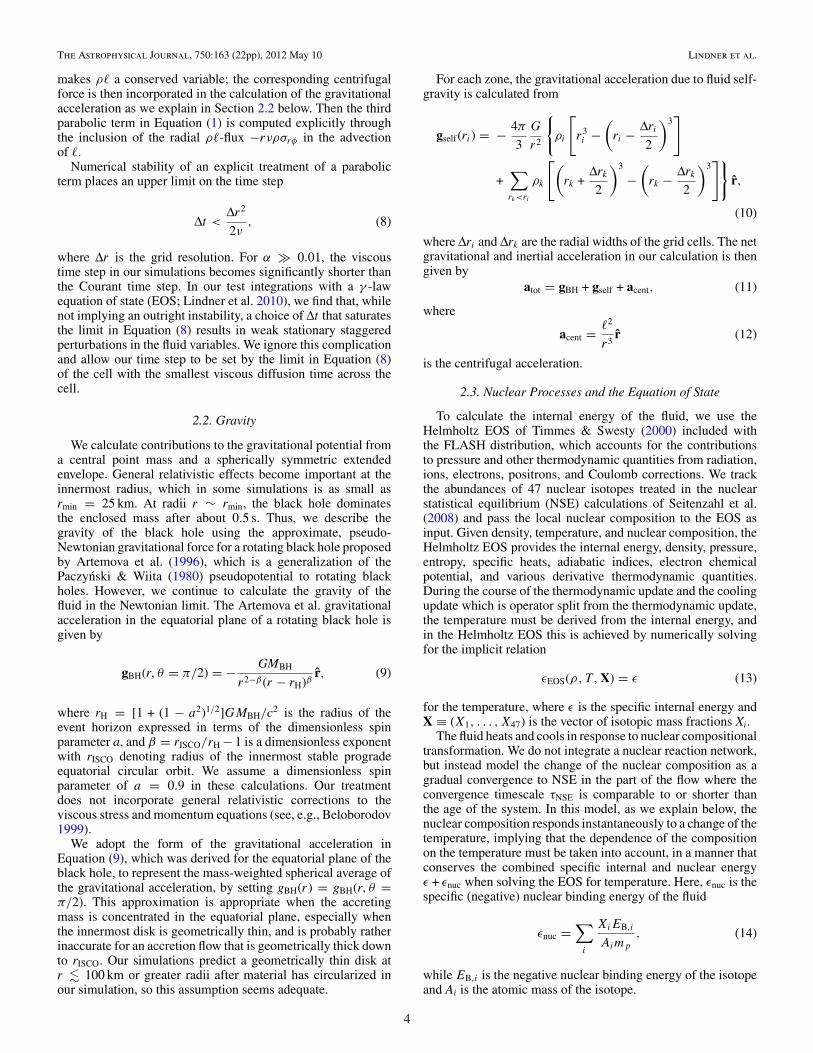
In Figure 1, we utilize Equation (50) to test the global conser-vation of internal energy in a run with identical test parametersto Run 2, except that we disabled nuclear compositional changeand used a Newtonian gravitational potential without relativisticcorrections. In the legend, the apparent error ΔE is defined asthe absolute value of the difference between the left- and right-hand sides of Equation (50). The evaluation of the various termsin Equation (50) was carried out in post-processing from cell-centered data recorded in Δt = 0.01 s intervals, which, in retro-spect, is prone to the introduction of various spatial and temporaldiscretization artifacts not present in the actual simulation.

We find that the apparent error is <1% of the largest termin Equation (50) when calculated for rmin,test = 50 km forthe time interval 0 s � t � 70 s. The apparent error is mostsignificant, ΔE ∼ 4 × 1050 erg, prior to and during the first fewseconds after shock passage. The apparent error that accruesafter the first few seconds following shock passage is less than1050 erg. This can be compared to the total binding energychange on the simulation grid, which if sufficiently large canimply a supernova. We calculate this energy in Section 3.5below and find that it increases by ∼(1.5–2)×1051 erg followingshock formation and a significant fraction (∼5 × 1050 erg) ofthe increase is accrued later than a few seconds after shockformation, when the change in the cumulative apparent erroris very small. Therefore, it does not seem that the apparentenergy conservation error at the levels seen in the simulationsshould significantly impact the prospects for explosion. We notethat in our calculations we explicitly transport specific internalenergy rather than the total energy, by setting the parametereintSwitch to a very large value. We would like to reiterate thatit is likely that the apparent error is an artifact of post-processingand the true energy conservation is better. To demonstrate thelatter, however, one would have to reconstruct the diagnosticenergy fluxes using the very same interpolation procedure as isperformed within the PPM in FLASH. We anticipate carryingout such a test in an extension of this work.

In steady state accretion, mass accretion associated withviscous angular momentum transport should occur at the rate

Ms.s. = −4π

(∂�

∂r

)−1∂

∂r

(r4νρ

∂Ω∂r

). (52)

8


Figure 1. Test of internal energy conservation in a run identical to Run 2 except with nuclear compositional change disabled and using a Newtonian gravitationalpotential. Plotted are each of the terms in Equation (50) calculated at rmin = 50 km (left) and rmin = 1000 km (right). Note the difference in scales on the verticalaxis. The quantity ΔE represents the absolute value of the difference between the left- and right-hand sides of Equation (50). A possibly dominant source of apparenterror is inconsistent discretization of the various fluid variables and fluxes in PPM and in the post-processing and need not reflect an inaccuracy of the computation.Neutrino losses are insignificant outside the inner ∼1000 km. Over the interval 0 s � t � 70 s, we find that the total error is <1% of the largest term in Equation (50).

(A color version of this figure is available in the online journal.)

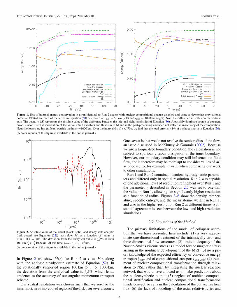
Figure 2. Absolute value of the actual (black, solid) and steady state analytic(red, dotted, see Equation (52)) mass flow, M , as a function of radius inRun 1 at t = 50 s. The deviation from the analytical value is �5% at radii100 km � r � 1000 km. At this time, rshock ∼ 7 × 104 km.


In Figure 2 we show M(r) for Run 2 at t = 50 s alongwith the analytic steady-state estimate of Equation (52). Inthe rotationally supported region 100 km � r � 1000 km,the deviation from the analytical value is �5%, which lendscredence to the accuracy of our angular momentum transportscheme.

Our spatial resolution was chosen such that we resolve theinnermost, neutrino-cooled region of the disk over several zones.

One caveat is that we do not resolve the sonic radius of the flow,an issue discussed in McKinney & Gammie (2002). Becausewe use a torque-free boundary condition, the calculation is notsubject to spurious viscous dissipation at the inner boundary.However, our boundary condition may still influence the fluidflow, and it therefore may be more apt to consider values of M ,as opposed to, for example, α or �, when comparing our workto other simulations.

Run 1 and Run 2 contained identical hydrodynamic parame-ters and differed only in spatial resolution. Run 2 was capableof one additional level of resolution refinement over Run 1 andthe parameter η described in Section 2.7 was set to one-halfthe value in Run 1, allowing for significantly higher resolutionas a function of radius. Figures 3–6 show the density, temper-ature, specific entropy, and the mean atomic weight in Run 1,and also in the higher-resolution Run 2 at different times. Sub-stantial agreement is seen between the low- and high-resolutionsimulations.

2.9. Limitations of the Method

The primary limitations of the model of collapsar accre-tion that we have presented here include: (1) a very approx-imate one-dimensional treatment of the intrinsically two- andthree-dimensional flow structures; (2) limited adequacy of theNavier–Stokes viscous stress as a model for the magnetic stressarising in the nonlinear development of the MRI; (3) no a pri-ori knowledge of the expected efficiency of convective energytransport ξconv and of compositional transport ξconv,mix; (4) treat-ment of nuclear compositional transformation through relax-ation to NSE rather than by integrating the nuclear reactionnetwork that would have allowed us to make predictions aboutthe nucleosynthetic output; (5) neglect of ambient composi-tional stratification and nuclear compositional transformationinside convective cells in the calculation of the convective heatflux; (6) the lack of modeling of the axial relativistic jet and

9


Figure 3. Density in Run 1 (left) and the higher resolution Run 2 (right) at t = 0 s (black, solid), t = 15 s (red, dotted), t = 25 s (green, dashed), and t = 50 s (blue,dash-dotted). In the convective region behind the shock front, some waves form due to an instability, developing at late times, which is likely an artifact of includingmixing length theory convection as an explicit term in the transport equations. The density jump across the shock front is approximately an order of magnitude.


Figure 4. Temperature in Run 1 (left) and the higher resolution Run 2 (right) at t = 0 s (black, solid), t = 15 s (red, dotted), t = 25 s (green, dashed), and t = 50 s(blue, dash-dotted). Photodisintegration and neutrino emission cool the innermost disk, while nuclear fusion provides additional heating in the post-shock region (seeSection 3.4).


its enveloping cocoon that are thought to be present in LRGBsources; and (7) the use of a relatively low mass progenitor star,which may or may not be able to yield a black hole and an explo-sion with an energy as high as has been inferred in supernovaeassociated with LGRBs. Overcoming limitations (1) through(6) will require much more computationally expensive multidi-mensional hydrodynamic and MHD simulations. Limitation (7)can be addressed by applying our current method to other, moremassive stellar models; here, we speculate what collapsars inhigher mass progenitors may behave like in Section 4 below.

It would be tempting in view of limitation (5) to try toincorporate the effects of compositional stratification ambient toconvective cells in the convective energy flux, which is normallyachieved by multiplying the energy flux in Equation (27) with afactor [

1 −(

dT

dμ

)P,ρ

dμ

dr

/ (T

cp

ds

dr

)]1/2

, (53)

where μ is the mean nuclear mass, and utilizing the Ledoux in-stead of the Schwarzschild criterion (see, e.g., Bisnovatyi-Kogan

10


Figure 5. Smoothed entropy ssmooth per baryon in Run 1 (left) and the higher resolution Run 2 (right) at t = 0 s (black, solid), t = 15 s (red, dotted), t = 25 s (green,dashed), and t = 50 s (blue, dash-dotted) in units of the Boltzmann constant (kB). After fluid comes into radial force balance, a strong entropy inversion is observed,giving rise to convection.


Figure 6. Mass-weighted average of the atomic mass A in Run 1 (left) and Run 2 (right) at t = 1 s (black, solid), t = 15 s (red, dotted), t = 25 s (green, dashed), andt = 50 s (blue, dot-dashed). Note that at t = 1 s, the iron core has already accreted onto the central point mass. At late times, photodisintegration in the hottest innerregions behind the shock front reduces the value of A. Convective mixing is able to dredge up lighter elements; our scheme for nuclear compositional transformationdoes not correctly model the subsequent recombination and freezeout well outside NSE.


2001). This would be meaningful as long as the convective eddyturnover time τconv ∼ λconv/vconv were shorter than the nucleartimescale τnuc � τNSE, so that the convective cells can be treatedas adiabatic before they mix. However, at radii where Ledouxconvection would differ most from Schwarzschild convection,namely, where the photodissociation into helium nuclei and freenucleons is substantial, the convective timescale is much longer

than the nuclear timescale, τconv � τnuc. The internal composi-tion of a convective cell evolves as it rises, and the associatedentropy change is a much stronger effect than the variation of theambient composition treated in Ledoux convection. Magnetiza-tion of the medium may play a role in this regime but its effectsare poorly understood. Research into the interplay of convec-tion and nuclear burning is ongoing (see, e.g., Arnett & Meakin

11


2011). Cognizant of these and other limitations, we adopt theSchwarzschild model and consider it but a parameterization ofcomplex, still-to-be-explored physics.

3. RESULTS

Nine simulations were carried out to explore sensitivity to theresolution of the simulation Δrmin, the viscous stress-to-pressureratio α, the stellar rotation ξ�, the efficiency of convective energytransport ξconv, and the efficiency of convective mixing ξconv,mix.The values of these parameters in each of the simulations aresummarized in Table 1. Among these, Run 1 can be consideredthe fiducial model. Each simulation was run for 100 s, except forRuns 4 and 5, where strong numerical instabilities associatedwith our convection scheme prevented us from simulating formore than 40 s and 50 s, respectively. In what follows, we presentthe results. In Section 3.1, we address the evolution of therate with which mass accretes onto the central black hole. InSection 3.2, we discuss the nature of radial force balance inthe fraction of the stellar material that has been traversed bythe outgoing shock wave, but has not accreted onto the blackhole and also discuss the mass and angular momentum transportin the system. In Section 3.3, we address energy transport. InSection 3.4, we address the nuclear composition of the flow anddiscuss the limitations inherent in our simplified treatment ofnuclear compositional transformation. In Section 3.5, we discussthe global energetics and check whether sufficient energy maybe transported into a portion of the stellar envelope to producea supernova.

3.1. Central Accretion Rate and Black Hole Mass

Each simulation exhibits unshocked radial accretion of theinner, low-angular momentum mass shells of the progenitorstar through the inner boundary lasting ∼(20–30) s at relativelysteady accretion rates of ∼(0.1–0.2) M� s−1. The central massaccretion rate, black hole mass, and total mass on the computa-tional grid as a function of time in each simulation are shownin Figure 7. The abrupt drop of the central accretion rate at∼(20–30) s is associated with the appearance of an accretionshock precipitated by the arrival of the mass shells with specificangular momentum sufficient to lead to circularization aroundthe black hole.

In Figure 8, we show the location of the shock rshock andits velocity vshock ≡ drshock/dt as a function of time. For eachof the runs, we identify the time when the shock first reachesradius 10 rmin = 250 km as the shock formation time tshock andlist the shock formation times in Column 2 of Table 2. We alsoprovide the mass of the black hole at this point, MBH(tshock), inColumn 8. The black hole mass at the time of shock formationwas MBH(tshock) ∼ (5.2–5.5) M� in Runs 1–7 and 9. In Run 8,which was initiated with reduced initial angular momentum,the accretion shock appeared later and the black hole mass iscorrespondingly larger.

After the formation of the shock, the fluid nearest the innerboundary is rotationally supported and accretes as a result ofangular momentum transport driven by the viscous shear stress.Subsequent to shock formation, the accretion rate declinesrapidly either promptly or following a short delay. The typicalrapid drop of the accretion rate is by a factor ∼5–10 (Runs 1,2, 3, 5, 7, and 9), and this is followed by a continued power-law-like decline. By the end of each simulation at 100 s, theaccretion rate has typically declined to ∼(10−3 − 10−4) M� s−1

(Runs 1, 2, 3, 4, 7, 8, and 9) or a factor of 100–1000 of the

Table 2Summary of Key Measurements

Run tshocka MBH(tshock)b Munbound

c Ebindd Ekin

e MFef

1 20.3 5.4 6.0 0.40 0.31 0.062g 19.1 5.2 6.4 0.44 0.36 0.043 19.2 5.2 5.7 0.34 0.28 0.064 19.8 5.3 4.4 0.62 0.29 0.075 20.6 5.5 3.1 0.40 0.18 0.046 20.3 5.4 0.0 −0.43 0.16 0.037 19.2 5.2 4.4 0.08 0.17 0.098 34.0 7.9 5.9 0.54 0.29 0.029 19.2 5.2 6.8 0.46 0.37 0.03

Notes.a Time at which shock reaches r = 250 km (s).b Black hole mass at when the shock reaches r = 250 kms (M�).c Unbound mass at the end of the simulation (M�).d Total energy in the stellar material at the end of the simulation (1051 erg s−1;see Section 3.5 and Figure 18).e Total kinetic energy of outbound material (1051 erg s−1; see Section 3.5).f Total mass of newly synthesized Fe-group elements at the end of the simulation(M�; see Section 3.4).g This run also had additional angular resolution (see Section 2.7).

pre-shock value. Final black hole masses were ∼(6–7) M� inthe simulations with ξ� = 0.5 and ∼10 M� in Run 8 withreduced initial angular momentum ξ� = 0.25.

In Run 4, with a low value of the viscosity parameter α =0.025, the shock first made a very slow progress from 300 km to2000 km during the first 10 s from its appearance. Then, at 30 s,the shock suddenly accelerated to vshock ∼ 5000 kms−1. Thenear-stagnation of the shock can be understood by noticing thatduring the 10 s, the neutrino cooling rate matches the viscousheating rate; the rapid cooling prevents the central entropy riseand convection seen in all other runs (see Section 3.3 below). InSection 4.2 of Lindner et al. (2010), we discussed the scenario inwhich the shock stagnation brought about by efficient neutrinocooling prolongs the LGRB central engine activity resulting ina longer prompt emission.

In Run 6, which had convective efficiency ξconv = 0.5, theshock stalled at the radius ∼104 km for ∼5 s before proceedingoutward. Note that the reinvigoration of the shock is solelydriven by the convective energy transport, as we do not simulatethe negligible neutrino energy and momentum deposition. Thestalling and restarting of the shock was reflected in a strongvariability of the central accretion rate.

3.2. The Shocked Envelope and Angular Momentum

Shock passage leaves a shock- and convection-heated, pres-sure supported envelope which contains much more mass thanthe disk, consistent with what we saw in Lindner et al. (2010).Figure 3 shows that the density in the envelope is an approxi-mate power law of radius ρ ∝ r−0.9. Figure 4 indicates that thetemperature is also a power-law T ∝ r−0.4. The pressure (notshown) is an approximate power law P ∝ r−1.8. The profilesextend inward into the regime in which rotational support dom-inates pressure support. The mass of the rotationally supportedmaterial in the grid, where acent > (1/2)|gself + gBH|, promptlyfollowing disk formation was typically �5% of the total masson the grid. Most of the mass on the grid was in the pressure sup-ported atmosphere seamlessly connecting to the disk. The massof the disk in each simulation is shown in Figure 7. In some ofthe runs, certain variability is seen in the disk mass over the firstfew seconds of disk formation. Afterward, the disk mass in each

12


Figure 7. Mass of the stellar envelope (top, black, solid), mass of the central object (top, red, dashed), mass of the disk (middle) as defined in Section 3.1, and massaccretion rate through the inner boundary (bottom) in each of the runs. Most of the mass is accreted onto the central object in the first ∼20 s in most runs. The diskmass makes up only a small portion of the total remaining, while the rest of the mass exists in a pressure supported atmosphere that may continue to feed the disk ormay be potentially unbound by the accretion shock. Plots of the disk mass begin when t = tshock. The quick drop in accretion rate seen in most of the simulationsoccurs around the time of shock formation.


13


Figure 8. Shock location (top) and velocity (bottom) in each of the runs. The red dashed line shows rdisk, the outermost radius where the acceleration due to thecentrifugal force is at least 50% the acceleration due to the pressure gradient. In Run 4 and Run 6, the shock stalls and is reinvigorated. Shock velocities were typically2000–4000 km s−1. The small fluctuations in the shock velocity are numerical artifacts of the discreteness in our shock detection algorithm.


simulation declines monotonically. In most runs (1–4 and 7–9)the disk mass declines to Mdisk � 10−5 M� by the end of thesimulation, while in Run 6, the mass at the end of the simulationis somewhat larger but still very small, Mdisk ∼ 3 × 10−4 M�.

Specific angular momentum as a function of radius is shownin Figure 9. In the initial angular momentum profile of themodel, compositional boundaries coincide with discontinuitiesin the profile, but in 16TI these occur only at mass coordinatesthat are accreted directly onto the black hole, prior to theinitial circularization. The angular momentum profile of themass shells remaining at initial circularization is monotonicallyincreasing and most of the remaining mass has nearly the same

angular momentum, ∼(1–2) × 1017 cm2 s−1.4 This implies thatthe shocked atmosphere has nearly uniform specific angularmomentum everywhere except at the radii where the timescaleon which the viscous torque transport angular momentum isshorter than the time since circularization. At (25–50) s, there isa mild, sub-Keplerian inward downturn in �(r) at r � 1000 km.Angular momentum transport is too slow within the initial∼100 s to affect the radii �104 km.

4 Stellar models exist in which nonmonotonicity is pronounced. This canproduce an interesting variability of the central accretion rate (e.g.,Lopez-Camara et al. 2010; Perna & MacFadyen 2010).

14


Figure 9. Specific angular momentum, �, as a function of radius in Run 1 att = 0 s (black, solid), t = 15 s (red, dotted), t = 25 s (green, dashed), andt = 50 s (blue, dot-dashed). The initial rotational profile for the stellar modelshows large spikes at compositional boundaries. Early in the simulation, lowangular momentum material is quickly accreted.


The mass accretion rate as a function of radius in Run 1 att = 50 s is shown in Figure 2. The accretion rate is independentof radius for r � 2000 km, which is the radii where the angularmomentum profile has relaxed to a viscous quasi-equilibrium.The analytic expectation, given in Equation (52), is shown aswell. Figure 10 shows the radial velocity vr , angular velocity vφ ,and Keplerian velocity as a function of radius at t = 18 s, just

as material begins to circularize outside of the black hole, andat t = 30 s, after an accretion disk has formed. At t = 18 s, thevelocity vφ reaches the Keplerian value at the innermost radii.

Throughout the simulations, we tracked the value of ourestimate of the vertical (z-directed) pressure scale height-to-radius ratio Hz/r , as described in Section 2.6. When theestimated ratio is below one-half, this indicates that in twodimensions, the flow should be disk-like, and when Hz/r 0.5,the flow is a geometrically thin disk. We found that Hz/ris below 0.5 but is still always above a minimum of 0.3everywhere, except in Run 4, which had the lowest viscosity. Thedisk-like radii where the vertical pressure scale height-to-radiusratio is below one-half are r � 200 km immediately followingcircularization and shrink to r � 100 km by the end of thesimulation. In Run 4 with a reduced viscous stress-to-pressureratio α, neutrino cooling drove the disk to be geometrically thin,where Hz/r � 0.3 in the inner r � 500 km. In the innermostzone in Run 4, Hz/r = 0.1 at t = 20 s, the lowest seen in anysimulation. By t = 35 s, no thin disk is present. In Figure 11 weshow the value of Ξmod defined in Equation (44) throughout thesimulation in Runs 1, 4, and 6; it does not drop below ∼0.77.Only in Run 4 is a genuinely thin accretion disk present, andthere it is limited to small radii. The outer radius of the thin diskdecreases as the neutrino luminosity drops (see Section 3.3).We attribute the observed moderate thinning of the accretionflow to the cooling of the flow by the photodisintegration ofhelium nuclei into free nucleons, and in Run 4, the additionalcontribution of neutrino cooling is also significant.

3.3. Energy Transport

To understand the energetics of the accretion flow in acollapsar, we need to consider the transport of mechanical,thermal, and nuclear binding energy, as well as the loss toneutrino emission. Before turning to energy transport, we

Figure 10. Absolute value of the radial velocity, vr (black, solid), Keplerian velocity including pseudo-relativistic corrections and self-gravity (red, dotted), and vφ

(green, dashed) as a function of radius in Run 1 at t = 18 s (left) and at t = 30 s (right), just as material begins to circularize. Note that the rotational velocity isapproaching the Keplerian velocity at the inner radii. Once material has become rotationally supported, there is a dramatic drop in vr . At radii 4000 km � r < rshock,the radial velocity is positive, indicating an outflow.


15


Figure 11. Value of the correction factor Ξmod applied to the temperature to account for the possibility of a reduced vertical scale height in, from left to right,Runs 1, 4, and 6 (see Section 2.6). This correction factor does not drop below ∼0.77 in any of the simulations, indicating that geometric thinning of the accretion flowis a relatively weak effect. The correction is only applied in regions where acent > 0.5 apres, which occurs only for r < 1000 km; thus Ξmod = 1.0 for r > 1000 km.


Figure 12. Neutrino luminosity integrated over the entire computational domainin representative Runs 1, 4, and 6 (see Section 2.4). The peak in luminosityoccurs shortly after the formation of the accretion shock. Note that we donot capture neutrino emission from the region r < 25 km, where muchneutronization and peak neutrino luminosity is expected to occur in the firstfew seconds after the formation and collapse of the iron core. The total neutrinoluminosities integrated over the entire simulation in Runs 1, 4, and 6 were 2.7,419.3, and 83.9 × 1051 erg, respectively.


discuss the neutrino losses, which turn out to be not significantin the regime we consider.

The integrated neutrino luminosity is dominated by the emis-sion from the inner ∼100 km. The luminosity as a function oftime in the representative Runs 1, 4, and 6 is shown in Figure 12.In simulations with α = 0.1, neutrino luminosities integratedover the entire computational domain peaked immediately fol-lowing shock formation at ∼(1–200) × 1051 erg s−1. The peakluminosity lasted anywhere from less than a second in the runswith high peak luminosities to a few seconds in the runs withlow peak luminosities. After the peak, the luminosity decays

first very rapidly until it has dropped to ∼1050 erg s−1, and thencontinues to decay approximately exponentially by several or-ders of magnitude to settle at ∼(10−6 to 10−5) erg s−1 after∼50 s. The sharp luminosity peak is an artifact of the abruptnature of shock formation in our 1.5D dimensional treatmentand is probably not physically significant. The total energy thatwould be deposited by an absorption of the emitted neutrinos,which we do not calculate, is negligible.

Now turning to energy transport, we examine the radial trans-port of all forms of energy, the thermal and kinetic energies, thenuclear binding energy, and the gravitational potential energy.The gravitational potential energy is a nonlocal functional ofthe mass distribution. However, ignoring relativistic effects, onecan define the gravitational potential energy per unit volume tobe ρ(ΦBH + (1/2)Φs), where ΦBH is the gravitational potentialof the black hole which we define via ΦBH(r) ≡ ∫ ∞

rgBH(r ′)dr ′

with gBH given in Equation (9) and Φself is that of the self-gravity of the star. Then, ρvrΦ, where Φ = ΦBH + Φself , can beinterpreted as the flux of gravitational energy advected by thefluid, but one must additionally include the flux of gravitationalenergy transported by self-gravity (see, e.g., Binney & Tremaine2008, their Appendix F), which equals

Fgrav,self = 1

8πG

(Φself∇ ∂Φself

∂t− ∂Φself

∂t∇Φself

). (54)

This term is significant only in the outer envelope of the star. Therate with which the sum total of these energies is transportedradially is given by

E = 4πr2

[ρvr

(ε + εnuc +

P

ρ+

1

2v2

r +1

2

�2

r2+ Φ

)+ Fgrav,self

− ρν�∂Ω∂r

+ Fconv + Fnuc,mix

], (55)

where the convention is such that E > 0 implies the transportof positive energy outward, opposite from the convectionemployed in the definition of the mass accretion rate M . Here,−ρν�∂Ω/∂r is flux of energy transported by the viscous stress.

Specific entropy as a function of radius at several timesin Runs 1 and 2 is shown in Figure 5. After the formationof the accretion shock and the rotationally supported flow,

16


Figure 13. Smoothed entropy ssmooth per baryon in units of the Boltzmannconstant (kB) at various times in the low-viscosity Run 4 (cf. Figure 5). Unlike inthe other runs, here a negative specific entropy gradient is not seen immediatelyafter the fluid comes into radial force balance. Even by t = 30 s the fluid is stillstable against convection; neutrino cooling prevents the early rise of convectiveinstability. Once the neutrino luminosity begins to drop around t = 33 s, entropyin the post-shock region begins to rise, bringing about strong entropy inversion.By the end of the simulation, Run 4 has the largest value of entropy seen in anyof the simulations.


viscous dissipation heats the fluid, thus producing a negativeentropy gradient in the shock downstream. The negative specificentropy gradient extends almost to the shock front, and thus theenergy injected at small radii can travel to raise the entropyof the entire post-shock region. Figure 13 shows the specificentropy in Run 4. Here, the high neutrino luminosity after theaccretion shock has formed keeps the entropy in the post shockregion relatively low. For the first ∼10 s after shock formation,no specific entropy inversion is seen, and the fluid is stableagainst convection. When the neutrino luminosity begins to droparound t ≈ 33 s, the entropy rises, a negative specific entropygradient appears in the post-shock region, and convection startstransporting the viscously dissipated energy outward.

Figure 14 plots the net transport rate E and the various con-stituent terms in Run 2 at t = 30 s; the radii and other ob-servables quoted in the remainder of this section will be spe-cific to this particular simulation snapshot and will vary acrossdifferent simulations and different times within a simulation.Approximate radial independence of the energy transport rate,∂E/∂r ≈ 0 for 200 km � r � 4000 km, where the transportrate is positive E ≈ 1050 erg s−1 > 0, is indicative of quasi-steady-state accretion. At larger radii, r � 5000 km, wherethe inner inflow gives way to an outer outflow—a precursorof the brewing explosion—no quasi-steady state is present andthe fluid variables evolve on the dynamical time in the wake ofthe expanding shock. At small radii, r � 100 km, where oneexpects a steady state, the curve E(r) exhibits a small positivegradient, as well as a sawtooth consistent with that seen in theaccretion rate M(r). The constancy of the plotted energy trans-port rate is contingent on an accurate cancellation of the othertransport terms. We suspect that the observed nonconstancy is

Figure 14. Total and partial energy transport rates in Run 2 at t = 30 s(see Section 3.3 and Equation (55)). The curves show E (black), the en-thalpy advection rate 4πr2vr (ρε + P ) (red), the kinetic energy advection rate2πr2vrρ(v2

r + �2/r2) (green), the gravitational potential energy transport rate4πr2(ρvrΦ + Fgrav,self ) (dark blue), the rate of energy transport by the viscousstress −4πr2ρν�∂Ω/∂r (pink), the rate of thermal energy transport by con-vection 4πr2Fconv (green), the nuclear energy transport rate associated withconvective compositional mixing 4πr2Fnuc,mix (gray), and the nuclear bindingenergy advection rate 4πr2vrρεnuc (orange). Negative values are indicated bydotted lines.


arising from relatively small inconsistencies in the discretizationor gravitational source terms in FLASH and in the calculationof the gravitational energy during post-processing.

At r � 1000 km, the inward advection of thermal and kineticenergy dominates over the outward transport by convectionand the viscous stress. Therefore, the innermost flow is anadvection-dominated accretion flow (ADAF; Narayan & Yi1994, 1995; Blandford & Begelman 1999). At r � 1000 km, theoutward transport of thermal energy by convection dominatesthe inward transport by advection and this region is thus aconvection-dominated accretion flow (CDAF, see, e.g., Stoneet al. 1999; Igumenshchev et al. 2000; Blandford & Begelman2004). Inward nuclear binding energy advection and nuclearcompositional mixing both act to transport the total energyoutward if one counts the negative nuclear binding energy inthe total energy budget. Convection transports energy from theADAF–CDAF transition radius where the magnitude of theenthalpy advection flux ∼|vr (ρε + P )| equals the convectionflux Fconv to the shock radius rshock. In Figure 14 the former isat rADAF ≈ 1000 km and the latter is at rshock ≈ 3.5 × 104 km.In Run 1 and similar runs, rADAF increases very slowly from∼1000 km to ∼2000 km from shock formation until t = 100 s.In Run 4, the radius is ∼200 km throughout the simulation, andin Run 6, the radius grows from ∼5000 km to over ∼104 km inthe course of the simulation.

We suspect that the location of rADAF determines the amountof energy that can be carried to the shock front, and that inturn, the ADAF–CDAF transition radius is primarily a functionof the convective efficiency ξconv and the viscous stress-to-pressure ratio α. Simulations with larger values of ξconv resulted

17


Figure 15. Abundances of the common elements summed over all isotopic species at (left to right) t = 0, 15, 25, 50 s in Run 1.


in stronger shocks and larger amounts of unbound material. Theconvective compositional mixing parameter ξconv,mix had littleeffect on the final outcome of our simulations. Turning to theviscosity parameter, Run 3 with a large values of α produceda somewhat less energetic shock with less unbound materialat the end of the simulation. Run 4, the simulation with thelowest viscosity, produced the most energetic explosion, evenin the presence of more pervasive cooling by neutrino emissionand by photodisintegration in the low-α regime; these flowsare denser and hotter (see, e.g., Popham et al. 1999; Chen &Beloborodov 2007). In Milosavljevic et al. (2012), we show thatrADAF is expected to be smaller under low viscosity conditionsbecause the advective luminosity is proportional to vr , whichis proportional to α. This trend is reproduced in the presentsimulations.

3.4. Nuclear Composition of the Flow

Our simplified treatment of nuclear compositional transfor-mation, which entails relaxation to NSE on a temperature-dependent timescale, is designed to track the impact of nuclearphotodisintegration and recombination on the thermodynamicsof the flow. However, it does not allow the computation of theultimate nucleosynthetic output in the presence of out-of-NSEburning. Thus, the results presented here can only be understoodin light of the limitations of the method.5 It is also worth recall-ing that we do not calculate neutronization that could modifythe proton-to-nucleon ratio Ye.

In the hottest, innermost accretion flow, photodisintegrationof heavy nuclei saps energy that could otherwise be transportedby convection to larger radii to energize the shocked envelope.However, once the nuclei are broken down, convective mixingcan dredge up free nucleons to larger and cooler radii, wherethey can recombine and heat the fluid locally. Figure 6 showsthe mean atomic mass A as a function of radius at varioustimes in Run 1 and Run 2. The mean atomic mass dropsbelow 4 in the innermost (200–300) km. The positive gradientin A seen in portions of the convective region would inthe Ledoux picture enhance the convective energy flux, butour Schwarzchild treatment of convection does not capturethis effect. We argue in Section 2.9 that since the nuclear

5 Metzger (2012) modeled accretion disks associated with the mergers ofwhite dwarfs and neutron stars or black holes. He found that nuclear processestaking place at temperatures T � 4 × 109 K may lead to significant heating inthe resulting outflows. The relaxation to NSE we employ underestimates theheating due to out-of-NSE nuclear recombination.

timescale is shorter than the convective timescale at radii whereLedoux convection implies an enhanced energy transport, thenuclear compositional transformation inside convective cells,not considered in the Ledoux treatment, should dominate.Lacking a theory of convection in this regime we adhere tothe simpler Schwarzschild parameterization.

In Figure 15, we show the mass-weighted abundances of themost common elements in our simulations in Run 1 at varioustimes. By t = 30 s, again, the inner 200 km is made up almostentirely of free nucleons in nearly equal portions, as Ye ≈ 0.5everywhere. The effect of convective compositional transportof the reprocessed nuclear species—the free nucleons, helium,and iron—from the hot innermost accretion flow is seen in thepower-law tails extending to near the location of the shock inthe right panels.

Although in our calculations we do not allow the evolutionof Ye, we can still speculate about the effects of neutronization.Chen & Beloborodov (2007) computed the structure of time-independent accretion disks around Kerr black holes includingthe effects of pair capture and neutronization. In their modelswith α = 0.1, the same as our fiducial viscous stress-to-pressureratio, at the radii where ρ ∼ 107 g cm−3, corresponding tothe density in the innermost disk in our simulations, they findYe ≈ 0.5, the same as in our non-neutronizing treatment. Intheir models with α = 0.01, however, Chen & Beloborodov(2007) find that at densities corresponding to the innermost diskin our simulations, significant neutronization was in effect andYe dropped well below neutron–proton equality. It is thereforepossible that in the very innermost regions of the disks in ourRun 4 with a low viscosity α = 0.025, the true value of Ye shouldbe lower than we assume. This would modify the abundancesand thermodynamics of the portion of the flow in NSE. The keyquestion of consequence for the viability of the mechanismwe propose for the production of luminous supernovae is,will the neutron-rich material pollute larger radii and drive atendency toward the synthesis of iron instead of 56Ni? Becausethis neutronization only seems to be most significant in thehottest innermost regions, where neutrino cooling is efficient andthe flow is predominantly rotationally supported, it is possiblethat most of the neutron-enhanced material would be advectedinto the black hole. This is a quantitative question that can beanswered only with multidimensional simulations.

In Figure 16, we show the location of rNSE, the largest radiusat which nuclear compositional transformation, in the form ofgradual convergence toward NSE, is taking place in our Run 1.This is the only region in which our calculations will capture

18


Figure 16. Location of rNSE, the largest radius at which nuclear compositionaltransformation, in the form of gradual convergence toward NSE, is taking placein our Run 1; this radius is closely approximated with the radius where thetemperature crosses ≈3 × 109 K.

nucleosynthesis and photodisintegration. Effectively, it is theradius at which T > 3 × 109 K. Early in the simulation, the hotstellar core accretes into the black hole, and rNSE quickly dropsfrom ≈3000 km to ≈800 km. After the shock forms, additionalheating in the shock and by viscous dissipation rapidly increasesrNSE and it peaks at ≈4000 km. As the density and temperaturedrop and the viscous heating rate decreases, the inner regions ofthe star begin to cool, and rNSE declines again.

In Figure 17, we show the total mass of various nuclear speciesin the entire simulation domain as a function of time. The mostnotable change is the dip in the mass of iron-group elements.The initial decrease in the iron-group mass is the accretion ofthe core of the star onto the black hole. After shock formation, arapid increase in the amount of free nucleons is seen, in additionto production of additional helium and iron-group elements. InTable 2, we show the total amount of newly fused Fe-groupelements present at the end of the simulation, which fall in therange of 0.02 M�–0.09 M�. Since we do not calculate the out-of-NSE burning in convectively dredged up material, at leasta fraction of the extended helium tail seen in Figure 15 couldbe expected to burn into iron and thus the iron-group mass inFigure 17 and Table 2 can be interpreted as a lower limit.

3.5. Prospects for Explosion

The total thermal and mechanical energy, which we also referto as the total binding energy, present on the grid was computedfor each simulation via

Ebind =∫ rmax

rmin

ρ

(ε +

1

2v2

r +1

2

�2

r2+ ΦBH +

1

2Φself

)4πr2dr

(56)and is shown in Figure 18. A positive binding energy indicatesa potential for explosion. Runs 1, 2, 3, 4, 5, 8, and 9 acquireda positive total binding energy Ebind ∼ (3.5–6.2) × 1050 ergby the end of the simulation, indicating the potential forexplosion. These runs have ξconv � 2 in common. Run 7

Figure 17. Mass of the most common elements summed over isotopic speciesin Run 1 as a function of time. Here, Fe represent all the isotopes of the irongroup. At the start of the simulation, there is a large dip in the amount of irongroup elements, due to the accretion of the iron core. After shock formation,∼0.05 M� of iron group elements are synthesized.


with ξconv = 1 reached marginally unbound condition withEbind ∼ (0.5–1) × 1050 erg. Run 6 with ξconv = 0.5 remainedgravitationally bound throughout the entire simulation.

The total unbound mass in each simulation was calculated bysumming the masses of any fluid element with a positive value ofEbind and a positive radial velocity. The total unbound masses ineach simulation defined by this diagnostic are shown in Table 2.This criterion does not take into account any interaction thatunbound and bound material might have subsequent to the mea-surement. This criterion also neglects future energy gain or lossfrom nuclear processes. The location and velocity of the outwardmoving accretion shock is shown in Figure 8. In exploding mod-els, the typical shock velocities were (2000–4000) km s−1. InRun 4 and Run 6, the shock stalled or slowed, and later restartedonce or several times. In Figure 19, we show the evolution ofvarious Lagrangian mass coordinates in Run 1 throughout thesimulation. Once the shock moves beyond ∼4000 km, the in-falling material obtains a positive velocity once it reaches rshock.

These results suggest that a high convective efficiency isrequired for sufficient transfer of energy from the inner accretionflow to the envelope to unbind the envelope. Simulations withhigher values of ξconv had relatively larger shock velocities andamounts of unbound mass at the ends of their simulations, andRun 4 with a lower α had the largest value of Ebind. Run 8with reduced initial specific angular momentum produced anexplosion comparable to that seen in the fiducial model.

4. OBSERVATIONAL SIGNATURESAND PROGENITOR TYPES

Modeling of light curves and spectra of supernovae associatedwith LGRBs has yielded information about the nature of theseexplosions. The mass of 56Ni present in the supernova ejectais easily estimated from the light curve by fitting simpleradioactive decay models. The velocity of the ejecta is inferred

19


Figure 18. Total binding energy on the simulation grid in Runs 1 and 2–9.Simulations in which the convective efficiency factor, ξconv � 0.5, reacheda positive total binding energy by the end of the simulation. The large, briefdips in energy visible in some simulations around the time of shock formationare primarily due to cooling by neutrino emission. The large dip seen inRun 4 is also predominantly due to neutrino cooling and has a minimum ofEbind = −1.5 × 1052 erg.

from observed line widths. Then, in a standard approach, thekinetic energy and mass of the ejecta are derived by comparingthe inferred 56Ni yield with that implied by one-dimensionalhydrodynamic models in which a spherical shock wave isintroduced by hand (by the action of a hypothetical “piston”)into the progenitor’s envelope.6 This approach relies on thehypothesis that 56Ni is produced at the shock front, for whichthe shock must be very strong.

Our simplified simulations suggest an alternative scenario inwhich nucleosynthesis takes place in the accretion flow in the

6 In “piston” and “thermal bomb” models, an explosion is mimicked byinjecting a large kinetic or thermal energy into a narrow shell over a relativelyshort �1 s time interval (e.g., Jones et al. 1981; Woosley & Weaver 1986;Arnett 1987; Shigeyama et al. 1987; Woosley et al. 1988; Thielemann et al.1990; Woosley & Weaver 1995; Limongi & Chieffi 2003; Chieffi & Limongi2004; Young & Fryer 2007; Fryer et al. 2008; Kasen & Woosley 2009; Maeda& Tominaga 2009; Joggerst et al. 2010; Dessart et al. 2011).

Figure 19. Evolution of the Lagrangian mass coordinates in Run 1 (black, solid).The location of rshock is also shown (red, dashed). The bifurcation between aninner inflow and an outer outflow occurs at r ∼ 4000 km. This corresponds toa mass coordinate of ∼5.6 M�.


interior of the star, similar to the wind-nucleosynthesis models(e.g., Beloborodov 2003; Pruet et al. 2003, 2004; Nagataki et al.2006; Surman et al. 2006; Maeda & Tominaga 2009; Metzger2012). Our results, however, suggest that the accretion flow islong lived, lasting tens or hundreds of seconds or longer, andso the nucleosynthesis can be sustained at lower densities thanin the wind models, and its products can be delivered to theenvelope by vigorous convection.

We also find that a supernova-like shock wave may be pow-ered by the sustained input of accretion energy, without ener-gization by neutrino energy deposition. The dynamics of theaccretion-energy-powered shock wave is fundamentally differ-ent from that powered by a piston. It remains to be exploredwhether the accretion scenario will call for a modification of thestandard approach to modeling the light curves and spectra of thesupernovae that could be yielding black holes. We are thus some-what reluctant to compare our results directly with observationalinferences obtained with existing supernova models. Previouswork has attributed kinetic energies of ∼(2–50)×1051 erg to su-pernovae associated with LGRBs (see, e.g., Woosley & Bloom2006; Hjorth & Bloom 2011, and references therein). Our mod-els come short of these energies, but they are consistent withthe low energy end among the more typical Type Ib and Icsupernovae (see, e.g., Table 4 in Hamuy 2003). Unfortunatelythe simplified treatment of nuclear compositional transforma-tion does not allow us to predict the 56Ni synthesized in ourmodels. We can only say that supernovae powered by collapsaraccretion should exhibit a high degree of mixing of hydrostaticand explosive elements.

The shock velocities at t = 100 s, when the shock is still inthe interior of the envelope, in the models that achieve explo-sion, are vshock ≈ 4000 km s−1. This is a half or smaller fractionof the commonly cited values for shock velocities measuredin the observed supernovae. Of course, leading to the break-out of the stellar surface, the shock accelerates as it traversesthe negative density gradient. The mass-weighted rms free

20


expansion velocity inferred from the total energy at the end of thesimulation is vFE ∼ (2Ebind/Munbound)1/2 ∼ 3000 (Ebind/0.5 ×1051 erg)1/2(Munbound/5 M�)−1/2 km s−1, again lower than usu-ally quoted for the observed supernovae.

Our initial model of choice was the Mstar ≈ 14 M�W-R model star 16TI of Woosley & Heger (2006), evolvedto pre-core-collapse from a 16 M� main-sequence progenitor.The model 16TI is commonly used in LGRB investigations(e.g., Morsony et al. 2007, 2010; Lopez-Camara et al. 2009,2010; Lazzati et al. 2010, 2011a, 2011b; Lindner et al. 2010;Nagakura et al. 2011a, 2011b), but it has been suggested thatthe progenitors of supernovae with confirmed association withLGRBs must be associated with the core collapse of more mas-sive stars, perhaps with masses in the range of (25–60) M� orhigher (e.g., Podsiadlowski et al. 2004; Smartt 2009, and ref-erences therein). However, predictions regarding the nature ofthe final remnant in such explosions are sensitive to the highlydebated details of the explosion mechanisms in core collapsesupernovae. Observational studies of the spatial distribution ofType Ic supernovae and GRBs in galaxies suggest that the re-spective progenitors should be at least ∼25 M� and ∼43 M�(Raskin et al. 2008; see also Larsson et al. 2007). It is of inter-est to note that simulations of neutron-star-powered explosionshave been successful only in the lowest mass progenitors. Theaccretion powered mechanism we propose will operate in moremassive progenitors that produce black holes. It is reasonable tospeculate that in progenitors more massive than in our model, orwith different internal structure, the explosion energies wouldbe much higher than we find, more in line with the high energiesof the LGRB supernovae. The long-term accretion in massivecollapsar progenitors deserves further study.

5. CONCLUSIONS

We have conducted a series of hydrodynamic simulations ofthe viscous post-core-collapse accretion of a rapidly rotating∼14 M� W-R star of Woosley & Heger (2006) onto the centralblack hole that we assumed was in place at the beginning ofthe simulation. The spherically symmetric simulations withrotation were carried out for 100 s and resolved the radii down to25 km, including the range of radii where the collapsing stellarmaterial circularizes around the black hole. The simulationstracked cooling by neutrino emission and the relaxation to NSEin the hot inner accretion flow. The simulations also trackedconvection and convective compositional mixing in the mixinglength theory approximation. Finally, the simulations trackedviscous angular momentum transport and the associated heatingin the flow. To explore the sensitivity to model parameters, wevaried the initial angular momentum profile, convective energytransport and compositional mixing efficiencies, and the viscousstress-to-pressure ratio α. Our main findings are as follows.

Lacking sufficient angular momentum to be rotationallysupported around the black hole, the inner mass coordinatesof the stellar envelope accrete unshocked onto the black hole.At t ∼ 20 s, or later with reduced initial angular momentum, thefirst mass shell able to circularize around the black hole arrives.Once material becomes circularized, an accretion shock formsas the mass shells in near free fall interact with the rotationallysupported material.

This shock front travels outward, leaving behind a mostlypressure supported, shock heated, convective stellar envelope.Only a very small fraction of the mass is predominantlyrotationally supported; the rotationally supported, geometricallythick disk connects smoothly to the pressure supported, shock-

heated envelope. The structure and energetics of the flow aregoverned by accretion mechanics. The energy dissipated by theviscous stress at the innermost radii, the radii smaller than somecritical rADAF, is advected into the black hole. The innermostflow is thus an ADAF. At larger radii, convection transports thedissipated energy outward, into the stellar envelope and towardthe expanding shock front, implying that the outer flow is aCDAF. The delivery of energy from ∼rADAF to the envelopeproceeds for tens of seconds, and the total energies deliveredare sufficient to produce supernovae, albeit not as energetic asthe ones inferred in association with LRGBs.

We found that the final energy deposited into the envelopestrongly depended on the efficiency of convective energy trans-port and depended somewhat on the viscous stress-to-pressureratio α. These two parameters strongly influence the location ofthe ADAF/CDAF transition, as we have explored with crudeanalytical arguments in Milosavljevic et al. (2012). The low-αmodel has a hotter disk with more pervasive cooling by neu-trino emission and nuclear photodisintegration, sapping energyfrom the final explosion. However, the low-α disk also has anADAF/CDAF transition at a smaller radius, potentially allow-ing for a higher convective luminosity.

For sufficiently high convective efficiencies, the stellar enve-lope was capable of obtaining positive total thermal and mechan-ical energies ∼0.5 × 1051 erg, shock velocities ∼4000 km s−1,and unbound masses ∼6 M�. We suggest that the accretionpowered mechanism, which is distinct from and possibly mutu-ally exclusive with the standard neutron-star-powered “delayed-neutrino” mechanism, could explain low-luminosity Type Ib andIc supernovae, but multidimensional study is needed to pin downthe true efficiency of convective energy transport and to estimatethe expected 56Ni yield.

We thank J. Craig Wheeler for helpful comments on a draftof this manuscript, and Rodolfo Barniol Duran, Lars Bildsten,Adam Burrows, Emmanouil Chatzopoulos, and Sean Couch forvaluable conversations. The software used in this work was inpart developed by the DOE-supported ASC/Alliance Centerfor Astrophysical Thermonuclear Flashes at the Universityof Chicago. The authors acknowledge the Texas AdvancedComputing Center (TACC) at the University of Texas at Austinfor providing high-performance computing resources that havecontributed to this research. C.C.L. acknowledges support froma National Science Foundation Graduate Research Fellowship.M.M. acknowledges support from NSF grants AST-0708795and AST-1009928. P.K. acknowledges support from NSF grantAST-0909110.

REFERENCES

Arnett, W. D. 1987, ApJ, 319, 136Arnett, W. D., & Meakin, C. 2011, ApJ, 733, 78Artemova, I. V., Bjoernsson, G., & Novikov, I. D. 1996, ApJ, 461, 565Balbus, S. A., & Hawley, J. F. 1998, Rev. Mod. Phys., 70, 1Balbus, S. A., & Hawley, J. F. 2002, ApJ, 573, 749Beloborodov, A. M. 1999, in ASP Conf. Ser. 161, High Energy Processes in

Accreting Black Holes, ed. J. Poutanen & R. Svensson (San Francisco, CA:ASP), 295

Beloborodov, A. M. 2003, ApJ, 588, 931Bethe, H. A., & Wilson, J. R. 1985, ApJ, 295, 14Binney, J., & Tremaine, S. (ed.) 2008, Galactic Dynamics (2nd ed.; Princeton,

NJ: Princeton Univ. Press)Bisnovatyi-Kogan, G. S. 1971, SvA, 14, 652Bisnovatyi-Kogan, G. S. 2001, in Stellar Physics. Vol. 1: Fundamental Concepts

and Stellar Equilibrium, ed. A. Y. Blinov & M. Romanova (Astronomy andAstrophysics Library, Translated from the Russian; Berlin: Springer), 323

21

http://dx.doi.org/10.1086/165439

http://adsabs.harvard.edu/abs/1987ApJ...319..136A


http://dx.doi.org/10.1088/0004-637X/733/2/78

http://adsabs.harvard.edu/abs/2011ApJ...733...78A

http://adsabs.harvard.edu/abs/2011ApJ...733...78A

http://dx.doi.org/10.1086/177084



http://dx.doi.org/10.1103/RevModPhys.70.1

http://adsabs.harvard.edu/abs/1998RvMP...70....1B

http://adsabs.harvard.edu/abs/1998RvMP...70....1B

http://dx.doi.org/10.1086/340767

http://adsabs.harvard.edu/abs/2002ApJ...573..749B


http://adsabs.harvard.edu/abs/1999ASPC..161..295B

http://dx.doi.org/10.1086/374217



http://dx.doi.org/10.1086/163343

http://adsabs.harvard.edu/abs/1985ApJ...295...14B

http://adsabs.harvard.edu/abs/1985ApJ...295...14B

http://adsabs.harvard.edu/abs/1971SvA....14..652B

http://adsabs.harvard.edu/abs/1971SvA....14..652B

http://adsabs.harvard.edu/abs/2001spfc.book.....B


Blandford, R. D., & Begelman, M. C. 1999, MNRAS, 303, L1Blandford, R. D., & Begelman, M. C. 2004, MNRAS, 349, 68Bloom, J. S., Kulkarni, S. R., Price, P. A., et al. 2002, ApJ, 572, L45Bucciantini, N., Quataert, E., Arons, J., Metzger, B. D., & Thompson, T. A.

2007, MNRAS, 380, 1541Bucciantini, N., Quataert, E., Arons, J., Metzger, B. D., & Thompson, T. A.

2008, MNRAS, 383, L25Bucciantini, N., Quataert, E., Metzger, B. D., et al. 2009, MNRAS, 396, 2038Buras, R., Janka, H.-T., Rampp, M., & Kifonidis, K. 2006a, A&A, 457, 281Buras, R., Rampp, M., Janka, H.-T., & Kifonidis, K. 2006b, A&A, 447, 1049Burrows, A. 1986, ApJ, 300, 488Burrows, A., Dessart, L., Livne, E., Ott, C. D., & Murphy, J. 2007, ApJ, 664,

416Calder, A. C., Townsley, D. M., Seitenzahl, I. R., et al. 2007, ApJ, 656, 313Campana, S., Mangano, V., Blustin, A. J., et al. 2006, Nature, 442, 1008Chen, W.-X., & Beloborodov, A. M. 2007, ApJ, 657, 383Chieffi, A., & Limongi, M. 2004, ApJ, 608, 405Chornock, R., Berger, E., Levesque, E. M., et al. 2010, arXiv:1004.2262Christodoulou, D. M., Contopoulos, J., & Kazanas, D. 2003, ApJ, 586, 372Cloutman, L. D., & Eoll, J. G. 1976, ApJ, 206, 548Cobb, B. E., Bloom, J. S., Perley, D. A., et al. 2010, ApJ, 718, L150Della Valle, M., Chincarini, G., Panagia, N., et al. 2006, Nature, 444, 1050Della Valle, M., Malesani, D., Benetti, S., et al. 2003, A&A, 406, L33Dessart, L., Burrows, A., Livne, E., & Ott, C. D. 2008, ApJ, 673, L43Dessart, L., Hillier, D. J., Livne, E., et al. 2011, MNRAS, 414, 2985Di Matteo, T., Perna, R., & Narayan, R. 2002, ApJ, 579, 706Fryer, C. L., Young, P., Bennett, M., et al. 2008, arXiv:0811.4648Fryxell, B., Olson, K., Ricker, P., et al. 2000, ApJS, 131, 273Fujimoto, S.-i., Kotake, K., Yamada, S., Hashimoto, M.-a., & Sato, K. 2006, ApJ,

644, 1040Galama, T. J., Tanvir, N., Vreeswijk, P. M., et al. 2000, ApJ, 536, 185Galama, T. J., Vreeswijk, P. M., van Paradijs, J., et al. 1998, Nature, 395, 670Garnavich, P. M., Stanek, K. Z., Wyrzykowski, L., et al. 2003, ApJ, 582, 924Hamuy, M. 2003, ApJ, 582, 905Heger, A., Fryer, C. L., Woosley, S. E., Langer, N., & Hartmann, D. H. 2003, ApJ,

591, 288Hjorth, J., & Bloom, J. S. 2011, in Gamma-Ray Bursts, ed. C. Kouveliotou,

R. A. M. J. Wijers, & S. E. Woosley (Cambridge: Cambridge Univ. Press),chapter 9, in press

Hjorth, J., Sollerman, J., Mller, P., et al. 2003, Nature, 423, 847Igumenshchev, I. V. 2002, ApJ, 577, L31Igumenshchev, I. V., Abramowicz, M. A., & Narayan, R. 2000, ApJ, 537, L27Igumenshchev, I. V., Narayan, R., & Abramowicz, M. A. 2003, ApJ, 592, 1042Iwamoto, K., Mazzali, P. A., Nomoto, K., et al. 1998, Nature, 395, 672Joggerst, C. C., Almgren, A., Bell, J., et al. 2010, ApJ, 709, 11Jones, E. M., Smith, B. W., & Straka, W. C. 1981, ApJ, 249, 185Kasen, D., & Woosley, S. E. 2009, ApJ, 703, 2205Kawabata, K. S., Deng, J., Wang, L., et al. 2003, ApJ, 593, L19Khokhlov, A. M. 1991, A&A, 245, 114Kohri, K., Narayan, R., & Piran, T. 2005, ApJ, 629, 341Kuhfuß, R. 1986, A&A, 160, 116Kumar, P., Narayan, R., & Johnson, J. L. 2008a, Science, 321, 376Kumar, P., Narayan, R., & Johnson, J. L. 2008b, MNRAS, 388, 1729Landau, L. D., & Lifshitz, E. M. 1959, Fluid Mechanics (Oxford: Pergamon)Larsson, J., Levan, A. J., Davies, M. B., & Fruchter, A. S. 2007, MNRAS, 376,

1285Lazzati, D., Blackwell, C. H., Morsony, B. J., & Begelman, M. C.

2011a, MNRAS, 411, L16Lazzati, D., Morsony, B. J., & Begelman, M. C. 2010, ApJ, 717, 239Lazzati, D., Morsony, B. J., & Begelman, M. C. 2011b, ApJ, 732, 34Lee, W. H., & Ramirez-Ruiz, E. 2006, ApJ, 641, 961Limongi, M., & Chieffi, A. 2003, ApJ, 592, 404Lindner, C. C., Milosavljevic, M., Couch, S. M., & Kumar, P. 2010, ApJ, 713,

800Lopez-Camara, D., Lee, W. H., & Ramirez-Ruiz, E. 2009, ApJ, 692, 804Lopez-Camara, D., Lee, W. H., & Ramirez-Ruiz, E. 2010, ApJ, 716, 1308MacFadyen, A. I., & Woosley, S. E. 1999, ApJ, 524, 262MacFadyen, A. I., Woosley, S. E., & Heger, A. 2001, ApJ, 550, 410Maeda, K., & Tominaga, N. 2009, MNRAS, 394, 1317

Malesani, D., Tagliaferri, G., Chincarini, G., et al. 2004, ApJ, 609, L5Marek, A., & Janka, H.-T. 2009, ApJ, 694, 664Matheson, T., Garnavich, P. M., Stanek, K. Z., et al. 2003, ApJ, 599, 394Mazzali, P. A., Deng, J., Pian, E., et al. 2006, ApJ, 645, 1323Mazzali, P. A., Deng, J., Tominaga, N., et al. 2003, ApJ, 599, L95McKinney, J. C., & Gammie, C. F. 2002, ApJ, 573, 728Metzger, B. D. 2012, MNRAS, 419, 827Mezzacappa, A., Bruenn, S. W., Blondin, J. M., Hix, W. R., & Bronson Messer,

O. E. 2007, in AIP Conf. Ser. 924, The Multicolored Landscape of CompactObjects and Their Explosive Origins (Melville, NY: AIP), 234

Milosavljevic, M., Lindner, C. C., Shen, R., & Kumar, P. 2012, ApJ, 744, 103Mirabal, N., Halpern, J. P., An, D., Thorstensen, J. R., & Terndrup, D. M.

2006, ApJ, 643, L99Modjaz, M., Stanek, K. Z., Garnavich, P. M., et al. 2006, ApJ, 645, L21Morsony, B. J., Lazzati, D., & Begelman, M. C. 2007, ApJ, 665, 569Morsony, B. J., Lazzati, D., & Begelman, M. C. 2010, ApJ, 723, 267Murphy, J. W., & Burrows, A. 2008, ApJ, 688, 1159Murphy, J. W., & Meakin, C. 2011, ApJ, 742, 74Nagakura, H., Ito, H., Kiuchi, K., & Yamada, S. 2011a, ApJ, 731, 80Nagakura, H., Suwa, Y., & Ioka, K. 2011b, arXiv:1104.5691Nagataki, S., Mizuta, A., & Sato, K. 2006, ApJ, 647, 1255Narayan, R., & Yi, I. 1994, ApJ, 428, L13Narayan, R., & Yi, I. 1995, ApJ, 444, 231Nordhaus, J., Burrows, A., Almgren, A., & Bell, J. 2010, ApJ, 720, 694Nousek, J. A., Kouveliotou, C., Grupe, D., et al. 2006, ApJ, 642, 389O’Brien, P. T., Willingale, R., Osborne, J., et al. 2006, ApJ, 647, 1213O’Connor, E., & Ott, C. D. 2010, Class. Quantum Grav., 27, 114103Paczynski, B., & Wiita, P. J. 1980, A&A, 88, 23Perna, R., & MacFadyen, A. 2010, ApJ, 710, L103Pian, E., Mazzali, P. A., Masetti, N., et al. 2006, Nature, 442, 1011Podsiadlowski, P., Mazzali, P. A., Nomoto, K., Lazzati, D., & Cappellaro, E.

2004, ApJ, 607, L17Popham, R., Woosley, S. E., & Fryer, C. 1999, ApJ, 518, 356Pruet, J., Thompson, T. A., & Hoffman, R. D. 2004, ApJ, 606, 1006Pruet, J., Woosley, S. E., & Hoffman, R. D. 2003, ApJ, 586, 1254Raskin, C., Scannapieco, E., Rhoads, J., & Della Valle, M. 2008, ApJ, 689, 358Reichart, D. E. 1999, ApJ, 521, L111Ryu, D., & Goodman, J. 1992, ApJ, 388, 438Scheck, L., Kifonidis, K., Janka, H.-T., & Muller, E. 2006, A&A, 457, 963Seitenzahl, I. R., Timmes, F. X., Marin-Lafleche, A., et al. 2008, ApJ, 685, L129Sekiguchi, Y., & Shibata, M. 2011, ApJ, 737, 6Shakura, N. I., & Sunyaev, R. A. 1973, A&A, 24, 337Shigeyama, T., Nomoto, K., Hashimoto, M., & Sugimoto, D. 1987, Nature, 328,

320Smartt, S. J. 2009, ARA&A, 47, 63Soderberg, A. M., Nakar, E., Berger, E., & Kulkarni, S. R. 2006, ApJ, 638, 930Stanek, K. Z., Matheson, T., Garnavich, P. M., et al. 2003, ApJ, 591, L17Starling, R. L. C., Wiersema, K., Levan, A. J., et al. 2011, MNRAS, 411, 2792Stone, J. M., & Balbus, S. A. 1996, ApJ, 464, 364Stone, J. M., Pringle, J. E., & Begelman, M. C. 1999, MNRAS, 310, 1002Surman, R., McLaughlin, G. C., & Hix, W. R. 2006, ApJ, 643, 1057Tagliaferri, G., Goad, M., Chincarini, G., et al. 2005, Nature, 436, 985Taylor, P. A., Miller, J. C., & Podsiadlowski, P. 2011, MNRAS, 410, 2385Thielemann, F.-K., Hashimoto, M.-A., & Nomoto, K. 1990, ApJ, 349, 222Thompson, T. A., Chang, P., & Quataert, E. 2004, ApJ, 611, 380Thompson, T. A., Quataert, E., & Burrows, A. 2005, ApJ, 620, 861Timmes, F. X., & Swesty, F. D. 2000, ApJS, 126, 501Wheeler, J. C., Yi, I., Hoflich, P., & Wang, L. 2000, ApJ, 537, 810Woosley, S. E. 1993, ApJ, 405, 273Woosley, S. E., & Bloom, J. S. 2006, ARA&A, 44, 507Woosley, S. E., & Heger, A. 2006, ApJ, 637, 914Woosley, S. E., & MacFadyen, A. I. 1999, A&AS, 138, 499Woosley, S. E., Pinto, P. A., & Ensman, L. 1988, ApJ, 324, 466Woosley, S. E., & Weaver, T. A. 1995, ApJS, 101, 181Woosley, S. E., & Weaver, T. A. 1986, ARA&A, 24, 205Young, P. A., & Fryer, C. L. 2007, ApJ, 664, 1033Zhang, W., Woosley, S. E., & Heger, A. 2008, ApJ, 679, 639Zimmerman, E. R., Narayan, R., McClintock, J. E., & Miller, J. M. 2005, ApJ,

618, 832

22

http://dx.doi.org/10.1046/j.1365-8711.1999.02358.x

http://adsabs.harvard.edu/abs/1999MNRAS.303L...1B

http://adsabs.harvard.edu/abs/1999MNRAS.303L...1B

http://dx.doi.org/10.1111/j.1365-2966.2004.07425.x

http://adsabs.harvard.edu/abs/2004MNRAS.349...68B

http://adsabs.harvard.edu/abs/2004MNRAS.349...68B

http://dx.doi.org/10.1086/341551

http://adsabs.harvard.edu/abs/2002ApJ...572L..45B

http://adsabs.harvard.edu/abs/2002ApJ...572L..45B

http://dx.doi.org/10.1111/j.1365-2966.2007.12164.x

http://adsabs.harvard.edu/abs/2007MNRAS.380.1541B


http://dx.doi.org/10.1111/j.1745-3933.2007.00403.x

http://adsabs.harvard.edu/abs/2008MNRAS.383L..25B

http://adsabs.harvard.edu/abs/2008MNRAS.383L..25B

http://dx.doi.org/10.1111/j.1365-2966.2009.14940.x



http://dx.doi.org/10.1051/0004-6361:20054654

http://adsabs.harvard.edu/abs/2006A&A...457..281B

http://adsabs.harvard.edu/abs/2006A&A...457..281B

http://dx.doi.org/10.1051/0004-6361:20053783

http://adsabs.harvard.edu/abs/2006A&A...447.1049B

http://adsabs.harvard.edu/abs/2006A&A...447.1049B

http://dx.doi.org/10.1086/163826



http://dx.doi.org/10.1086/519161



http://dx.doi.org/10.1086/510709

http://adsabs.harvard.edu/abs/2007ApJ...656..313C


http://dx.doi.org/10.1038/nature04892

http://adsabs.harvard.edu/abs/2006Natur.442.1008C

http://adsabs.harvard.edu/abs/2006Natur.442.1008C

http://dx.doi.org/10.1086/508923



http://dx.doi.org/10.1086/392523



http://www.arxiv.org/abs/1004.2262

http://dx.doi.org/10.1086/367615



http://dx.doi.org/10.1086/154411



http://dx.doi.org/10.1088/2041-8205/718/2/L150

http://adsabs.harvard.edu/abs/2010ApJ...718L.150C

http://adsabs.harvard.edu/abs/2010ApJ...718L.150C


http://adsabs.harvard.edu/abs/2006Natur.444.1050D

http://adsabs.harvard.edu/abs/2006Natur.444.1050D

http://dx.doi.org/10.1051/0004-6361:20030855

http://adsabs.harvard.edu/abs/2003A&A...406L..33D

http://adsabs.harvard.edu/abs/2003A&A...406L..33D

http://dx.doi.org/10.1086/527519

http://adsabs.harvard.edu/abs/2008ApJ...673L..43D

http://adsabs.harvard.edu/abs/2008ApJ...673L..43D

http://dx.doi.org/10.1111/j.1365-2966.2011.18598.x

http://adsabs.harvard.edu/abs/2011MNRAS.414.2985D

http://adsabs.harvard.edu/abs/2011MNRAS.414.2985D

http://dx.doi.org/10.1086/342832

http://adsabs.harvard.edu/abs/2002ApJ...579..706D

http://adsabs.harvard.edu/abs/2002ApJ...579..706D


http://dx.doi.org/10.1086/317361

http://adsabs.harvard.edu/abs/2000ApJS..131..273F

http://adsabs.harvard.edu/abs/2000ApJS..131..273F

http://dx.doi.org/10.1086/503624

http://adsabs.harvard.edu/abs/2006ApJ...644.1040F

http://adsabs.harvard.edu/abs/2006ApJ...644.1040F

http://dx.doi.org/10.1086/308909

http://adsabs.harvard.edu/abs/2000ApJ...536..185G


http://dx.doi.org/10.1038/27150

http://adsabs.harvard.edu/abs/1998Natur.395..670G

http://adsabs.harvard.edu/abs/1998Natur.395..670G

http://dx.doi.org/10.1086/344785



http://dx.doi.org/10.1086/344689

http://adsabs.harvard.edu/abs/2003ApJ...582..905H


http://dx.doi.org/10.1086/375341




http://adsabs.harvard.edu/abs/2003Natur.423..847H

http://adsabs.harvard.edu/abs/2003Natur.423..847H

http://dx.doi.org/10.1086/344148

http://adsabs.harvard.edu/abs/2002ApJ...577L..31I


http://dx.doi.org/10.1086/312755



http://dx.doi.org/10.1086/375769

http://adsabs.harvard.edu/abs/2003ApJ...592.1042I

http://adsabs.harvard.edu/abs/2003ApJ...592.1042I

http://dx.doi.org/10.1038/27155

http://adsabs.harvard.edu/abs/1998Natur.395..672I

http://adsabs.harvard.edu/abs/1998Natur.395..672I

http://dx.doi.org/10.1088/0004-637X/709/1/11

http://adsabs.harvard.edu/abs/2010ApJ...709...11J

http://adsabs.harvard.edu/abs/2010ApJ...709...11J

http://dx.doi.org/10.1086/159274

http://adsabs.harvard.edu/abs/1981ApJ...249..185J

http://adsabs.harvard.edu/abs/1981ApJ...249..185J

http://dx.doi.org/10.1088/0004-637X/703/2/2205

http://adsabs.harvard.edu/abs/2009ApJ...703.2205K

http://adsabs.harvard.edu/abs/2009ApJ...703.2205K

http://dx.doi.org/10.1086/378148

http://adsabs.harvard.edu/abs/2003ApJ...593L..19K

http://adsabs.harvard.edu/abs/2003ApJ...593L..19K

http://adsabs.harvard.edu/abs/1991A&A...245..114K


http://dx.doi.org/10.1086/431354

http://adsabs.harvard.edu/abs/2005ApJ...629..341K

http://adsabs.harvard.edu/abs/2005ApJ...629..341K



http://dx.doi.org/10.1126/science.1159003

http://adsabs.harvard.edu/abs/2008Sci...321..376K

http://adsabs.harvard.edu/abs/2008Sci...321..376K

http://dx.doi.org/10.1111/j.1365-2966.2008.13493.x

http://adsabs.harvard.edu/abs/2008MNRAS.388.1729K

http://adsabs.harvard.edu/abs/2008MNRAS.388.1729K

http://dx.doi.org/10.1111/j.1365-2966.2007.11523.x

http://adsabs.harvard.edu/abs/2007MNRAS.376.1285L

http://adsabs.harvard.edu/abs/2007MNRAS.376.1285L

http://dx.doi.org/10.1111/j.1745-3933.2010.00984.x

http://adsabs.harvard.edu/abs/2011MNRAS.411L..16L

http://adsabs.harvard.edu/abs/2011MNRAS.411L..16L

http://dx.doi.org/10.1088/0004-637X/717/1/239

http://adsabs.harvard.edu/abs/2010ApJ...717..239L


http://dx.doi.org/10.1088/0004-637X/732/1/34

http://adsabs.harvard.edu/abs/2011ApJ...732...34L

http://adsabs.harvard.edu/abs/2011ApJ...732...34L

http://dx.doi.org/10.1086/500533



http://dx.doi.org/10.1086/375703



http://dx.doi.org/10.1088/0004-637X/713/2/800



http://dx.doi.org/10.1088/0004-637X/692/1/804



http://dx.doi.org/10.1088/0004-637X/716/2/1308

http://adsabs.harvard.edu/abs/2010ApJ...716.1308L

http://adsabs.harvard.edu/abs/2010ApJ...716.1308L

http://dx.doi.org/10.1086/307790

http://adsabs.harvard.edu/abs/1999ApJ...524..262M


http://dx.doi.org/10.1086/319698



http://dx.doi.org/10.1111/j.1365-2966.2009.14460.x

http://adsabs.harvard.edu/abs/2009MNRAS.394.1317M

http://adsabs.harvard.edu/abs/2009MNRAS.394.1317M

http://dx.doi.org/10.1086/422684

http://adsabs.harvard.edu/abs/2004ApJ...609L...5M

http://adsabs.harvard.edu/abs/2004ApJ...609L...5M

http://dx.doi.org/10.1088/0004-637X/694/1/664



http://dx.doi.org/10.1086/379228



http://dx.doi.org/10.1086/504415

http://adsabs.harvard.edu/abs/2006ApJ...645.1323M


http://dx.doi.org/10.1086/381259

http://adsabs.harvard.edu/abs/2003ApJ...599L..95M


http://dx.doi.org/10.1086/340761



http://dx.doi.org/10.1111/j.1365-2966.2011.19747.x

http://adsabs.harvard.edu/abs/2012MNRAS.419..827M

http://adsabs.harvard.edu/abs/2012MNRAS.419..827M

http://adsabs.harvard.edu/abs/2007AIPC..924..234M

http://dx.doi.org/10.1088/0004-637X/744/2/103



http://dx.doi.org/10.1086/505177



http://dx.doi.org/10.1086/505906



http://dx.doi.org/10.1086/519483



http://dx.doi.org/10.1088/0004-637X/723/1/267



http://dx.doi.org/10.1086/592214



http://dx.doi.org/10.1088/0004-637X/742/2/74

http://adsabs.harvard.edu/abs/2011ApJ...742...74M

http://adsabs.harvard.edu/abs/2011ApJ...742...74M

http://dx.doi.org/10.1088/0004-637X/731/2/80

http://adsabs.harvard.edu/abs/2011ApJ...731...80N

http://adsabs.harvard.edu/abs/2011ApJ...731...80N


http://dx.doi.org/10.1086/505618

http://adsabs.harvard.edu/abs/2006ApJ...647.1255N

http://adsabs.harvard.edu/abs/2006ApJ...647.1255N

http://dx.doi.org/10.1086/187381

http://adsabs.harvard.edu/abs/1994ApJ...428L..13N

http://adsabs.harvard.edu/abs/1994ApJ...428L..13N

http://dx.doi.org/10.1086/175599

http://adsabs.harvard.edu/abs/1995ApJ...444..231N


http://dx.doi.org/10.1088/0004-637X/720/1/694



http://dx.doi.org/10.1086/500724



http://dx.doi.org/10.1086/505457

http://adsabs.harvard.edu/abs/2006ApJ...647.1213O

http://adsabs.harvard.edu/abs/2006ApJ...647.1213O

http://dx.doi.org/10.1088/0264-9381/27/11/114103

http://adsabs.harvard.edu/abs/2010CQGra..27k4103O

http://adsabs.harvard.edu/abs/2010CQGra..27k4103O

http://adsabs.harvard.edu/abs/1980A&A....88...23P

http://adsabs.harvard.edu/abs/1980A&A....88...23P

http://dx.doi.org/10.1088/2041-8205/710/2/L103

http://adsabs.harvard.edu/abs/2010ApJ...710L.103P

http://adsabs.harvard.edu/abs/2010ApJ...710L.103P


http://adsabs.harvard.edu/abs/2006Natur.442.1011P

http://adsabs.harvard.edu/abs/2006Natur.442.1011P

http://dx.doi.org/10.1086/421347

http://adsabs.harvard.edu/abs/2004ApJ...607L..17P

http://adsabs.harvard.edu/abs/2004ApJ...607L..17P

http://dx.doi.org/10.1086/307259

http://adsabs.harvard.edu/abs/1999ApJ...518..356P

http://adsabs.harvard.edu/abs/1999ApJ...518..356P

http://dx.doi.org/10.1086/382036

http://adsabs.harvard.edu/abs/2004ApJ...606.1006P


http://dx.doi.org/10.1086/367957



http://dx.doi.org/10.1086/592495

http://adsabs.harvard.edu/abs/2008ApJ...689..358R


http://dx.doi.org/10.1086/312203

http://adsabs.harvard.edu/abs/1999ApJ...521L.111R

http://adsabs.harvard.edu/abs/1999ApJ...521L.111R

http://dx.doi.org/10.1086/171165



http://dx.doi.org/10.1051/0004-6361:20064855

http://adsabs.harvard.edu/abs/2006A&A...457..963S

http://adsabs.harvard.edu/abs/2006A&A...457..963S

http://dx.doi.org/10.1086/592501

http://adsabs.harvard.edu/abs/2008ApJ...685L.129S

http://adsabs.harvard.edu/abs/2008ApJ...685L.129S

http://dx.doi.org/10.1088/0004-637X/737/1/6

http://adsabs.harvard.edu/abs/2011ApJ...737....6S

http://adsabs.harvard.edu/abs/2011ApJ...737....6S

http://adsabs.harvard.edu/abs/1973A&A....24..337S

http://adsabs.harvard.edu/abs/1973A&A....24..337S

http://dx.doi.org/10.1038/328320a0

http://adsabs.harvard.edu/abs/1987Natur.328..320S

http://adsabs.harvard.edu/abs/1987Natur.328..320S

http://dx.doi.org/10.1146/annurev-astro-082708-101737

http://adsabs.harvard.edu/abs/2009ARA&A..47...63S

http://adsabs.harvard.edu/abs/2009ARA&A..47...63S

http://dx.doi.org/10.1086/499121

http://adsabs.harvard.edu/abs/2006ApJ...638..930S


http://dx.doi.org/10.1086/376976

http://adsabs.harvard.edu/abs/2003ApJ...591L..17S

http://adsabs.harvard.edu/abs/2003ApJ...591L..17S

http://dx.doi.org/10.1111/j.1365-2966.2010.17879.x

http://adsabs.harvard.edu/abs/2011MNRAS.411.2792S


http://dx.doi.org/10.1086/177328



http://dx.doi.org/10.1046/j.1365-8711.1999.03024.x



http://dx.doi.org/10.1086/501116

http://adsabs.harvard.edu/abs/2006ApJ...643.1057S

http://adsabs.harvard.edu/abs/2006ApJ...643.1057S


http://adsabs.harvard.edu/abs/2005Natur.436..985T

http://adsabs.harvard.edu/abs/2005Natur.436..985T

http://dx.doi.org/10.1111/j.1365-2966.2010.17618.x

http://adsabs.harvard.edu/abs/2011MNRAS.410.2385T

http://adsabs.harvard.edu/abs/2011MNRAS.410.2385T

http://dx.doi.org/10.1086/168308

http://adsabs.harvard.edu/abs/1990ApJ...349..222T


http://dx.doi.org/10.1086/421969



http://dx.doi.org/10.1086/427177



http://dx.doi.org/10.1086/313304

http://adsabs.harvard.edu/abs/2000ApJS..126..501T

http://adsabs.harvard.edu/abs/2000ApJS..126..501T

http://dx.doi.org/10.1086/309055

http://adsabs.harvard.edu/abs/2000ApJ...537..810W


http://dx.doi.org/10.1086/172359



http://dx.doi.org/10.1146/annurev.astro.43.072103.150558

http://adsabs.harvard.edu/abs/2006ARA&A..44..507W


http://dx.doi.org/10.1086/498500



http://dx.doi.org/10.1051/aas:1999325

http://adsabs.harvard.edu/abs/1999A&AS..138..499W

http://adsabs.harvard.edu/abs/1999A&AS..138..499W

http://dx.doi.org/10.1086/165908



http://dx.doi.org/10.1086/192237

http://adsabs.harvard.edu/abs/1995ApJS..101..181W

http://adsabs.harvard.edu/abs/1995ApJS..101..181W

http://dx.doi.org/10.1146/annurev.aa.24.090186.001225



http://dx.doi.org/10.1086/518081

http://adsabs.harvard.edu/abs/2007ApJ...664.1033Y

http://adsabs.harvard.edu/abs/2007ApJ...664.1033Y

http://dx.doi.org/10.1086/526404

http://adsabs.harvard.edu/abs/2008ApJ...679..639Z


http://dx.doi.org/10.1086/426071



Documents

SIMULATIONS OF ACCRETION POWERED SUPERNOVAE IN …