Carlos R. Morrison and Andrew J. ProvenzaGlenn Research Center, Cleveland, Ohio

Simulink® Controller for a Reluctance MotorWith Four-Pole Rotor and 36-Tooth Stator

NASA/TP—2017-219451

May 2017

https://ntrs.nasa.gov/search.jsp?R=20170004841 2018-05-11T06:31:11+00:00Z

NASA STI Program . . . in Profi le

Since its founding, NASA has been dedicated to the advancement of aeronautics and space science. The NASA Scientifi c and Technical Information (STI) Program plays a key part in helping NASA maintain this important role.

The NASA STI Program operates under the auspices of the Agency Chief Information Offi cer. It collects, organizes, provides for archiving, and disseminates NASA’s STI. The NASA STI Program provides access to the NASA Technical Report Server—Registered (NTRS Reg) and NASA Technical Report Server—Public (NTRS) thus providing one of the largest collections of aeronautical and space science STI in the world. Results are published in both non-NASA channels and by NASA in the NASA STI Report Series, which includes the following report types: • TECHNICAL PUBLICATION. Reports of

completed research or a major signifi cant phase of research that present the results of NASA programs and include extensive data or theoretical analysis. Includes compilations of signifi cant scientifi c and technical data and information deemed to be of continuing reference value. NASA counter-part of peer-reviewed formal professional papers, but has less stringent limitations on manuscript length and extent of graphic presentations.

• TECHNICAL MEMORANDUM. Scientifi c

and technical fi ndings that are preliminary or of specialized interest, e.g., “quick-release” reports, working papers, and bibliographies that contain minimal annotation. Does not contain extensive analysis.

• CONTRACTOR REPORT. Scientifi c and technical fi ndings by NASA-sponsored contractors and grantees.

• CONFERENCE PUBLICATION. Collected papers from scientifi c and technical conferences, symposia, seminars, or other meetings sponsored or co-sponsored by NASA.

• SPECIAL PUBLICATION. Scientifi c,

technical, or historical information from NASA programs, projects, and missions, often concerned with subjects having substantial public interest.

• TECHNICAL TRANSLATION. English-

language translations of foreign scientifi c and technical material pertinent to NASA’s mission.

For more information about the NASA STI program, see the following:

• Access the NASA STI program home page at http://www.sti.nasa.gov

• E-mail your question to help@sti.nasa.gov • Fax your question to the NASA STI

Information Desk at 757-864-6500

• Telephone the NASA STI Information Desk at 757-864-9658 • Write to:

NASA STI Program Mail Stop 148 NASA Langley Research Center Hampton, VA 23681-2199

Carlos R. Morrison and Andrew J. ProvenzaGlenn Research Center, Cleveland, Ohio

Simulink® Controller for a Reluctance MotorWith Four-Pole Rotor and 36-Tooth Stator

NASA/TP—2017-219451

May 2017

National Aeronautics andSpace Administration

Glenn Research CenterCleveland, Ohio 44135

Acknowledgments

The motor technology and code discussed in this report were developed with support from the NASA Advanced Air Transportation Technologies (AATT) project (Amy Jankovsky, manager), and special recognition is extended to Dr. Gerald V. Brown for his many insightful discussions throughout this effort, and for suggesting the simple torque analysis to allow preliminary evaluation of candidate waveforms for stator coil current.

Available from

Trade names and trademarks are used in this report for identifi cation only. Their usage does not constitute an offi cial endorsement, either expressed or implied, by the National Aeronautics and

Space Administration.

Level of Review: This material has been technically reviewed by a committee of expert reviewer(s).

NASA STI ProgramMail Stop 148NASA Langley Research CenterHampton, VA 23681-2199

National Technical Information Service5285 Port Royal RoadSpringfi eld, VA 22161

703-605-6000

This report is available in electronic form at http://www.sti.nasa.gov/ and http://ntrs.nasa.gov/

This work was sponsored by the Advanced Air Vehicle Program at the NASA Glenn Research Center

NASA/TP—2017-219451 1

Simulink® Controller for a Reluctance Motor With Four-Pole Rotor and 36-Tooth Stator

Carlos R. Morrison and Andrew J. Provenza

National Aeronautics and Space Administration Glenn Research Center Cleveland, Ohio 44135

Summary

NASA Glenn Research Center has developed MathWorks® Simulink® controller logic for driving a room-temperature, 36-tooth stator, four-pole rotor reluctance motor. The Simulink® core logic was extracted from an existing C motor controller that was employed to achieve a rotor speed of 3000 rpm. The Simulink® controller, however, has significant additional logic refinements that were not available in the existing C controller, such as the “Per_Rev_Logic” component and its frequency filter. The filter provides a more accurate reading of the rotor input signals than the previous version of the controller. The controller is versatile, and with slight modifications, can be used to drive other reluctance motor types incorporating dissimilar stator and rotor pole combinations. The original C controller was designed with the goal (after appropriate modification) of controlling a future superconducting motor. This superconducting motor will be employed as a testbed for developing other superconducting aviation propulsion motors envisioned for future turboelectric aircraft. The Simulink® results presented in this paper were generated from simulated rotor inputs. However, in an actual application, these simulated inputs would be replaced by actual proximity probe signals.

Introduction

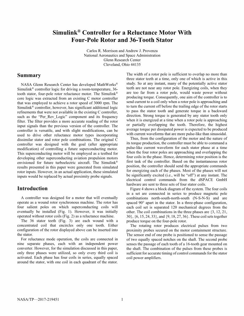
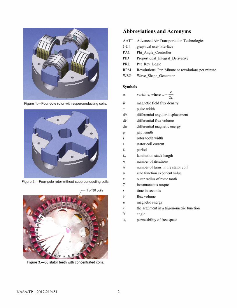
A controller was designed for a motor that will eventually operate as a wound rotor synchronous machine. The rotor has four salient poles on which superconducting coils will eventually be installed (Fig. 1). However, it was initially operated without rotor coils (Fig. 2) as a reluctance machine.

The 36 stator teeth (Fig. 3) are each wound with a concentrated coil that encircles only one tooth. Either configuration of the rotor displayed above can be inserted into the stator.

For reluctance mode operation, the coils are connected in nine separate phases, each with an independent power converter. However, for the simulation discussed in this paper, only three phases were utilized, so only every third coil is activated. Each phase has four coils in series, equally spaced around the stator, with one coil in each quadrant of the stator.

The width of a rotor pole is sufficient to overlap no more than three stator teeth at a time, only one of which is active in this study. So at any instant, many of the potentially active stator teeth are not near any rotor pole. Energizing coils, when they are too far from a rotor pole, would waste power without producing torque. Consequently, one aim of the controller is to send current to a coil only when a rotor pole is approaching and to turn the current off before the trailing edge of the rotor starts to pass the stator tooth and generate torque in a backward direction. Strong torque is generated by any stator tooth only when it is energized at a time when a rotor pole is approaching or partially overlapping the tooth. Therefore, the highest average torque per dissipated power is expected to be produced with current waveforms that are more pulse-like than sinusoidal.

Thus, from the configuration of the motor and the nature of its torque production, the controller must be able to command a pulse-like current waveform for each stator phase at a time when the four rotor poles are approaching and overlapping the four coils in the phase. Hence, determining rotor position is the first task of the controller. Based on the instantaneous rotor position, the controller should send the appropriate commands for energizing each of the phases. Most of the phases will not be significantly excited (i.e., will be “off”) at any instant. The electrical control commands from the dSPACE GmbH hardware are sent to three sets of four stator coils.

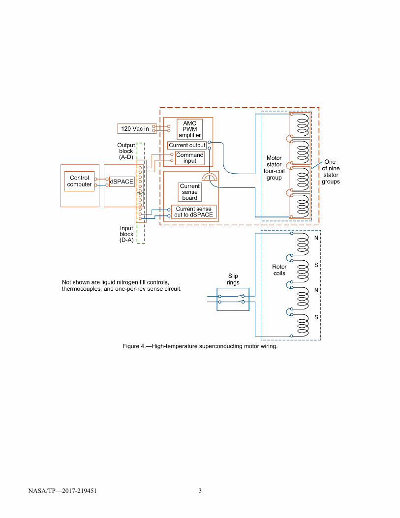
Figure 4 shows a block diagram of the system. The four coils in a set are connected in series to produce magnetic pole combinations north-south-north-south (N-S-N-S) and are spaced 90° apart in the stator. In a three-phase configuration, each coil set is separated 120 mechanical degrees from the other. The coil combinations in the three phases are {3, 12, 21, 30}, {6, 15, 24, 33}, and {9, 18, 27, 36}. These coil sets together produce torque on the four-pole rotor.

The rotating rotor produces electrical pulses from two proximity probes secured on the motor containment structure. The sensor end of one probe is positioned to sense the passage of two equally spaced notches on the shaft. The second probe senses the passage of each tooth of a 16-tooth gear mounted on the shaft. The combination of the pulses from these probes is sufficient for accurate timing of control commands for the stator coil power amplifiers.

NASA/TP—2017-219451 2

Figure 1.—Four-pole rotor with superconducting coils.

Figure 2.—Four-pole rotor without superconducting coils.

Figure 3.—36 stator teeth with concentrated coils.

Abbreviations and Acronyms

AATT Advanced Air Transportation Technologies

GUI graphical user interface

PAC Phi_Angle_Controller

PID Proportional_Integral_Derivative

PRL Per_Rev_Logic

RPM Revolutions_Per_Minute or revolutions per minute

WSG Wave_Shape_Generator

Symbols

a variable, where 2

ca

L

B magnetic field flux density

c pulse width

d differential angular displacement

dV differential flux volume

dw differential magnetic energy

g gap length

I rotor tooth width

i stator coil current

L period

Ls lamination stack length

n number of iterations

N number of turns in the stator coil

p sine function exponent value

r outer radius of rotor tooth

T instantaneous torque

t time in seconds

V flux volume

w magnetic energy

x the argument in a trigonometric function

angle

o permeability of free space

NASA/TP—2017-219451 3

Figure 4.—High-temperature superconducting motor wiring.

NASA/TP—2017-219451 4

Rotor-Stator Mechanical Depiction

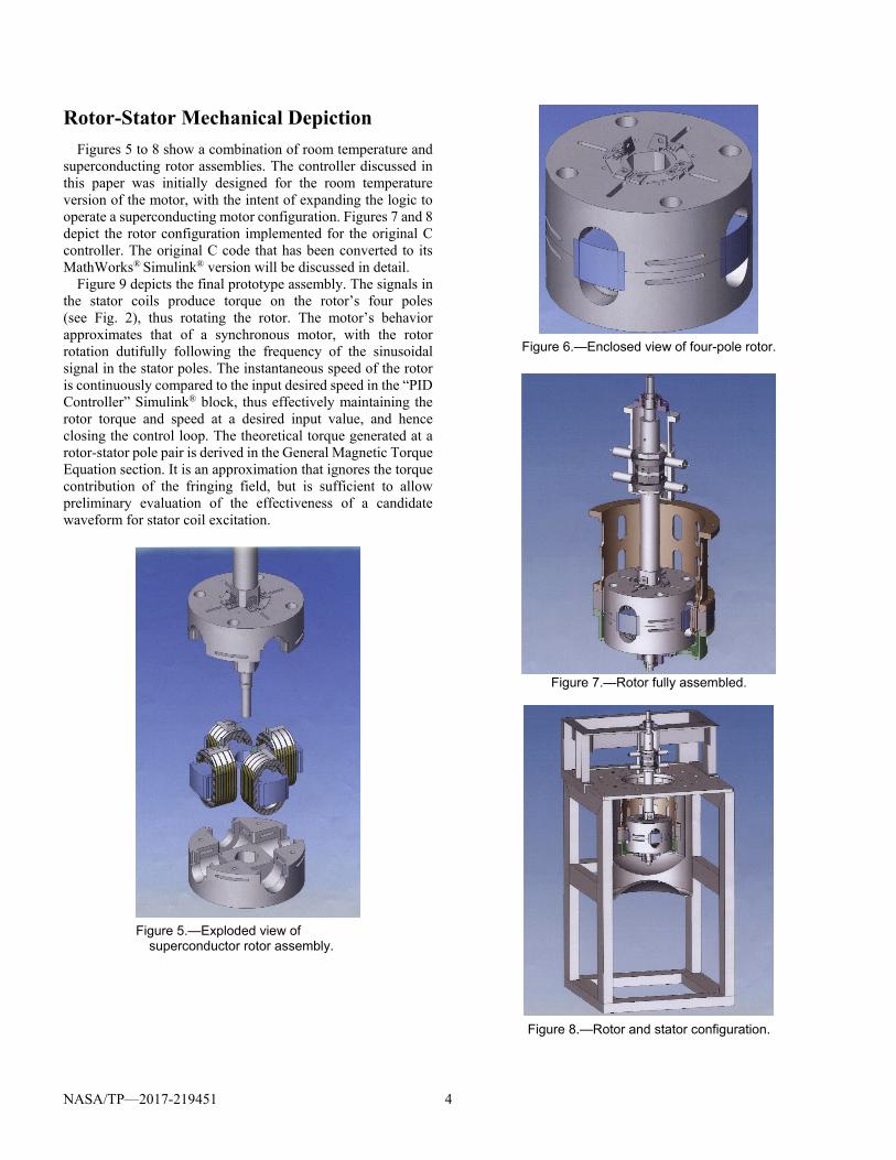
Figures 5 to 8 show a combination of room temperature and superconducting rotor assemblies. The controller discussed in this paper was initially designed for the room temperature version of the motor, with the intent of expanding the logic to operate a superconducting motor configuration. Figures 7 and 8 depict the rotor configuration implemented for the original C controller. The original C code that has been converted to its MathWorks® Simulink® version will be discussed in detail.

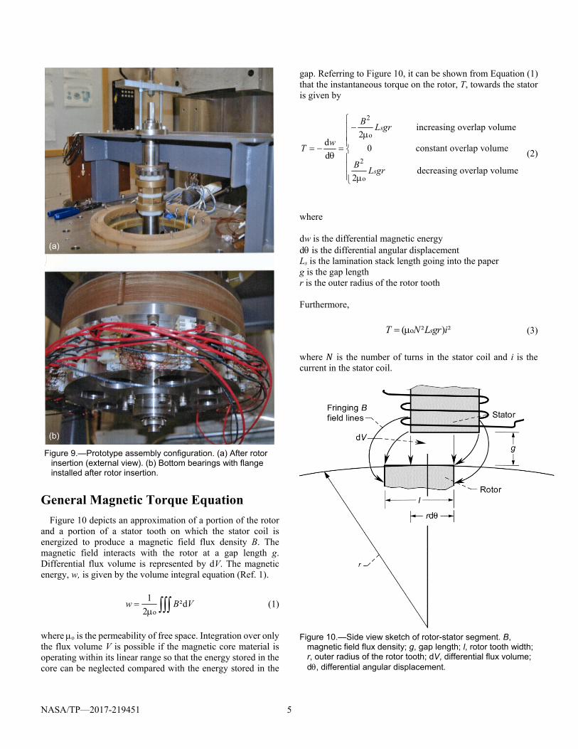
Figure 9 depicts the final prototype assembly. The signals in the stator coils produce torque on the rotor’s four poles (see Fig. 2), thus rotating the rotor. The motor’s behavior approximates that of a synchronous motor, with the rotor rotation dutifully following the frequency of the sinusoidal signal in the stator poles. The instantaneous speed of the rotor is continuously compared to the input desired speed in the “PID Controller” Simulink® block, thus effectively maintaining the rotor torque and speed at a desired input value, and hence closing the control loop. The theoretical torque generated at a rotor-stator pole pair is derived in the General Magnetic Torque Equation section. It is an approximation that ignores the torque contribution of the fringing field, but is sufficient to allow preliminary evaluation of the effectiveness of a candidate waveform for stator coil excitation.

Figure 5.—Exploded view of

superconductor rotor assembly.

Figure 6.—Enclosed view of four-pole rotor.

Figure 7.—Rotor fully assembled.

Figure 8.—Rotor and stator configuration.

NASA/TP—2017-219451 5

Figure 9.—Prototype assembly configuration. (a) After rotor

insertion (external view). (b) Bottom bearings with flange installed after rotor insertion.

General Magnetic Torque Equation

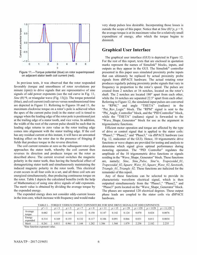
Figure 10 depicts an approximation of a portion of the rotor and a portion of a stator tooth on which the stator coil is energized to produce a magnetic field flux density B. The magnetic field interacts with the rotor at a gap length g. Differential flux volume is represented by dV. The magnetic energy, w, is given by the volume integral equation (Ref. 1).

o

1²d

2w B V

(1)

where o is the permeability of free space. Integration over only the flux volume V is possible if the magnetic core material is operating within its linear range so that the energy stored in the core can be neglected compared with the energy stored in the

gap. Referring to Figure 10, it can be shown from Equation (1) that the instantaneous torque on the rotor, T, towards the stator is given by

2

o

2

o

increasing overlap volume2

d0 constant overlap volume

d

decreasing overlap volume2

s

s

BL gr

wT

BL gr

(2)

where dw is the differential magnetic energy d is the differential angular displacement Ls is the lamination stack length going into the paper g is the gap length r is the outer radius of the rotor tooth Furthermore, o( ² ) ²sT N L gr i (3)

where is the number of turns in the stator coil and i is the current in the stator coil.

Figure 10.—Side view sketch of rotor-stator segment. B,

magnetic field flux density; g, gap length; l, rotor tooth width; r, outer radius of the rotor tooth; dV, differential flux volume; d, differential angular displacement.

NASA/TP—2017-219451 6

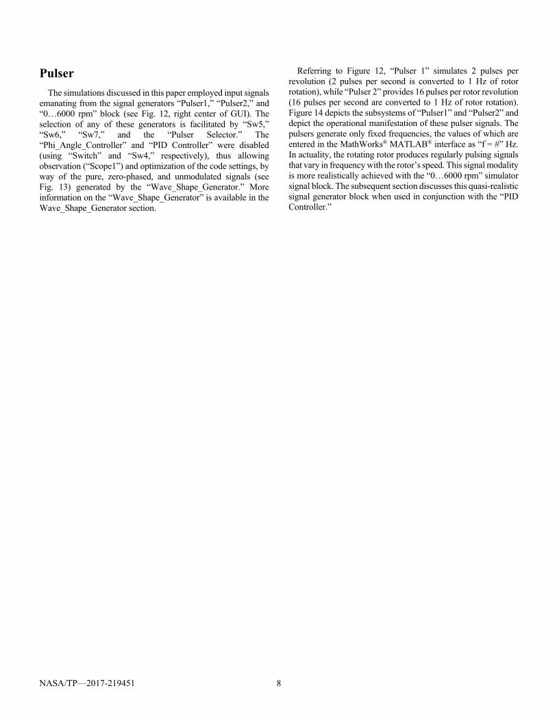
Figure 11.—Torque potential (blue) on rotor superimposed

on adjacent stator teeth coil current (red).

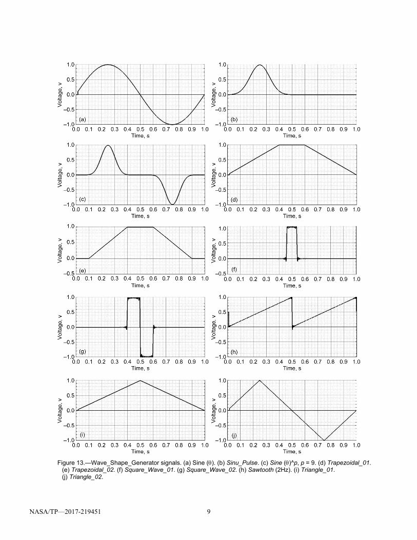
In previous tests, it was observed that the rotor responded favorably (torque and smoothness of rotor revolutions per minute (rpm)) to drive signals that are representative of sine signals of odd power exponents (see the red curve in Fig. 11, Sine ()^9, or triangular wave (Fig. 13(j)). The torque potential (blue), and coil current (red) curves versus nondimensional time are depicted in Figure 11. Referring to Figures 10 and 11, the maximum clockwise torque on a rotor’s pole is achieved when the apex of the current pulse (red) in the stator coil is timed to engage when the leading edge of the rotor pole is positioned just at the trailing edge of a stator tooth, and vice versa. In addition, the width of the root of the current pulse should be such that its leading edge returns to zero value as the rotor trailing edge comes into alignment with the stator trailing edge. If the coil has any residual current at this instant, it will have an unwanted braking effect on the rotor due to the presence of fringing B fields that produce torque in the reverse direction.

The coil current remains at zero as the subsequent rotor pole approaches the stator teeth, whereby the coil current then reverses its direction and produces torque on the rotor as described above. The current reversal switches the magnetic polarity in the stator teeth, thus having the beneficial effect of demagnetizing stator teeth and simultaneously maintaining the induced magnetic polarity in the rotor tooth. This electrical event occurs in all four coils in a set, and all three coil sets are energized simultaneously, thus producing continuous torque on the rotor. Table I depicts the calculated benefits (with the help of Mathematica) of using sine drive signals of odd exponents. The merit value is obtained by dividing the average torque by the expended energy.

The expended energy does not consider eddy-current losses in the iron core, which increase with frequency and would make

very sharp pulses less desirable. Incorporating those losses is outside the scope of this paper. Notice that at Sine ()^p, p = 9, the average torque is at its maximum value for a relatively small expenditure of energy, after which the torque begins to diminish.

Graphical User Interface

The graphical user interface (GUI) is depicted in Figure 12. For the rest of this report, texts that are enclosed in quotation marks represent the names of Simulink® blocks, inputs, and outputs as they appear in the GUI. The Simulink® controller presented in this paper uses simulated proximity probe inputs that can ultimately be replaced by actual proximity probe signals from dSPACE hardware. The actual rotating rotor produces regularly pulsing proximity probe signals that vary in frequency in proportion to the rotor’s speed. The pulses are created from 2 notches or 16 notches, located on the rotor’s shaft. The 2 notches are located 180° apart from each other, while the 16 notches are separated 22.5° apart from each other. Referring to Figure 12, the simulated input pulses are converted to “RPM,” and angle “THETA” (radians) in the “Per_Rev_Logic” block. The “RPM” signal is sent to the “Phi_Angle_Controller” block, and the “PID Controller” block, while the “THETA” (radians) signal is forwarded to the “Wave_Shape_Generator” block for use as the argument in trigonometric functions.

Efficient motor operation and torque are affected by the type of drive or control signal that is applied to the stator coils: “Phase1,” “Phase2,” and “Phase3,” via dSPACE hardware (see Fig. 12, midcenter of the GUI). Hence, 10 trigonometric drive functions or wave shapes are provided for testing and analysis to determine which signal gives optimal performance during motoring operation. The “PID Controller” regulates the amplitude of the 10 trigonometric drive functions or signals residing in the “Wave_Shape_Generator” block. These functions are, namely; Sine, Sinu_Pulse, Sine^n, Trapezoidal_01, Trapezoidal_02, Square_Wave_01, Square_Wave_02, Sawtooth, Triangle_01, Triangle_02. These functions are italicized for the remainder of this report.

Any of these functions can be selected to provide its characteristic waveform electrical signal, which is then outputted simultaneously from the “Phase1,” “Phase2,” and “Phase3” ports located on the “Wave_Shape_Generator” block. The phases are separated 120 electrical degrees. These output phase leads are coupled to the stator coils via dSPACE hardware.

TABLE I.—TORQUE VERSUS ENERGY EXPENDITURE FOR SINE DRIVE SIGNALS OF ODD EXPONENTS pa = 1 p = 3 p = 5 p = 7 p = 9 p = 11 p = 15 p = 29 p = 129 p = 1129 p = 11,129 Average torque

0.082 0.137 0.149 0.151 0.150 0.147 0.142 0.124 0.070 0.024 0.0076

Energy expended

0.314 0.169 0.155 0.132 0.117 0.106 0.091 0.066 0.031 0.011 0.0034

Merit 0.261 0.811 0.961 1.144 1.282 1.386 1.560 1.879 2.258 2.182 2.235 aSine function exponent value.

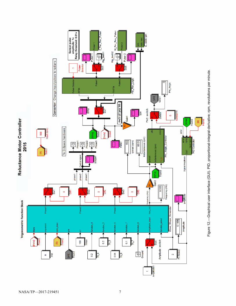
F

igur

e 1

2.—

Gra

phic

al u

ser

inte

rfac

e (G

UI)

. PID

, pro

port

iona

l-int

egr

al-d

eriv

ativ

e; r

pm, r

evol

utio

ns p

er m

inut

e.

NASA/TP—2017-219451 7

NASA/TP—2017-219451 8

Pulser

The simulations discussed in this paper employed input signals emanating from the signal generators “Pulser1,” “Pulser2,” and “0…6000 rpm” block (see Fig. 12, right center of GUI). The selection of any of these generators is facilitated by “Sw5,” “Sw6,” “Sw7,” and the “Pulser Selector.” The “Phi_Angle_Controller” and “PID Controller” were disabled (using “Switch” and “Sw4,” respectively), thus allowing observation (“Scope1”) and optimization of the code settings, by way of the pure, zero-phased, and unmodulated signals (see Fig. 13) generated by the “Wave_Shape_Generator.” More information on the “Wave_Shape_Generator” is available in the Wave_Shape_Generator section.

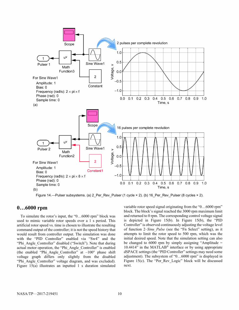
Referring to Figure 12, “Pulser 1” simulates 2 pulses per revolution (2 pulses per second is converted to 1 Hz of rotor rotation), while “Pulser 2” provides 16 pulses per rotor revolution (16 pulses per second are converted to 1 Hz of rotor rotation). Figure 14 depicts the subsystems of “Pulser1” and “Pulser2” and depict the operational manifestation of these pulser signals. The pulsers generate only fixed frequencies, the values of which are entered in the MathWorks® MATLAB® interface as “f = #” Hz. In actuality, the rotating rotor produces regularly pulsing signals that vary in frequency with the rotor’s speed. This signal modality is more realistically achieved with the “0…6000 rpm” simulator signal block. The subsequent section discusses this quasi-realistic signal generator block when used in conjunction with the “PID Controller.”

NASA/TP—2017-219451 9

Figure 13.—Wave_Shape_Generator signals. (a) Sine (). (b) Sinu_Pulse. (c) Sine ()^p, p = 9. (d) Trapezoidal_01.

(e) Trapezoidal_02. (f) Square_Wave_01. (g) Square_Wave_02. (h) Sawtooth (2Hz). (i) Triangle_01. (j) Triangle_02.

NASA/TP—2017-219451 10

Figure 14.—Pulser subsystems. (a) 2_Per_Rev_Pulser (1 cycle × 2). (b) 16_Per_Rev_Pulser (8 cycles × 2).

0…6000 rpm

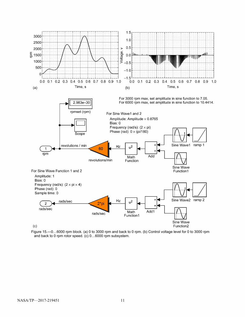
To simulate the rotor’s input, the “0…6000 rpm” block was used to mimic variable rotor speeds over a 1 s period. This artificial rotor speed vs. time is chosen to illustrate the resulting command output of the controller; it is not the speed history that would result from controller output. The simulation was done with the “PID Controller” enabled via “Sw4” and the “Phi_Angle_Controller” disabled (“Switch”). Note that during actual motor operation, the “Phi_Angle_Controller” is enabled (the enabled “Phi_Angle_Controller” at –100° phase shift voltage graph differs only slightly from the disabled “Phi_Angle_Controller” voltage diagram, and was excluded). Figure 15(a) illustrates an inputted 1 s duration simulated

variable rotor speed signal originating from the “0…6000 rpm” block. The block’s signal reached the 3000 rpm maximum limit and returned to 0 rpm. The corresponding control voltage signal is depicted in Figure 15(b). In Figure 15(b), the “PID Controller” is observed continuously adjusting the voltage level of function 2–Sinu_Pulse (see the “Fn Select” setting), as it attempts to limit the rotor speed to 500 rpm, which was the initial desired speed. Note that the simulation setting can also be changed to 6000 rpm by simply assigning “Amplitude = 10.4414” in the MATLAB® interface or by using appropriate dSPACE settings (the “PID Controller” settings may need some adjustment). The subsystem of “0…6000 rpm” is displayed in Figure 15(c). The “Per_Rev_Logic” block will be discussed next.

NASA/TP—2017-219451 11

Figure 15.—0…6000 rpm block. (a) 0 to 3000 rpm and back to 0 rpm. (b) Control voltage level for 0 to 3000 rpm

and back to 0 rpm rotor speed. (c) 0…6000 rpm subsystem.

NASA/TP—2017-219451 12

Per_Rev_Logic

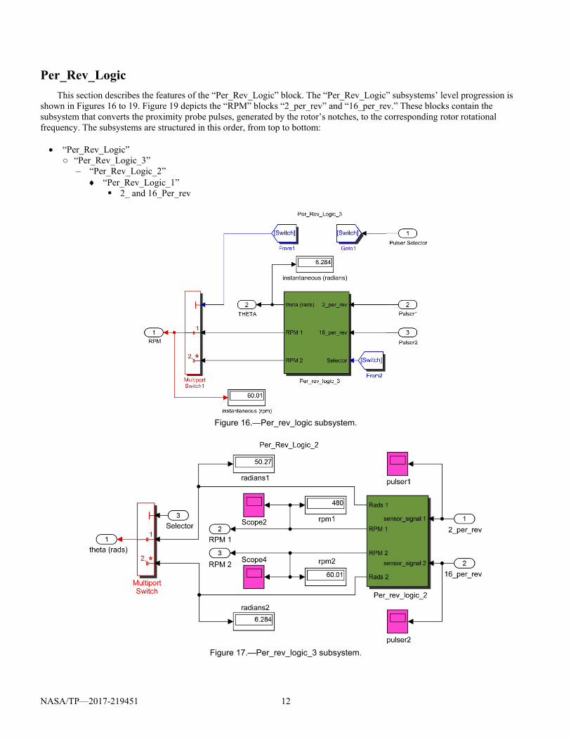
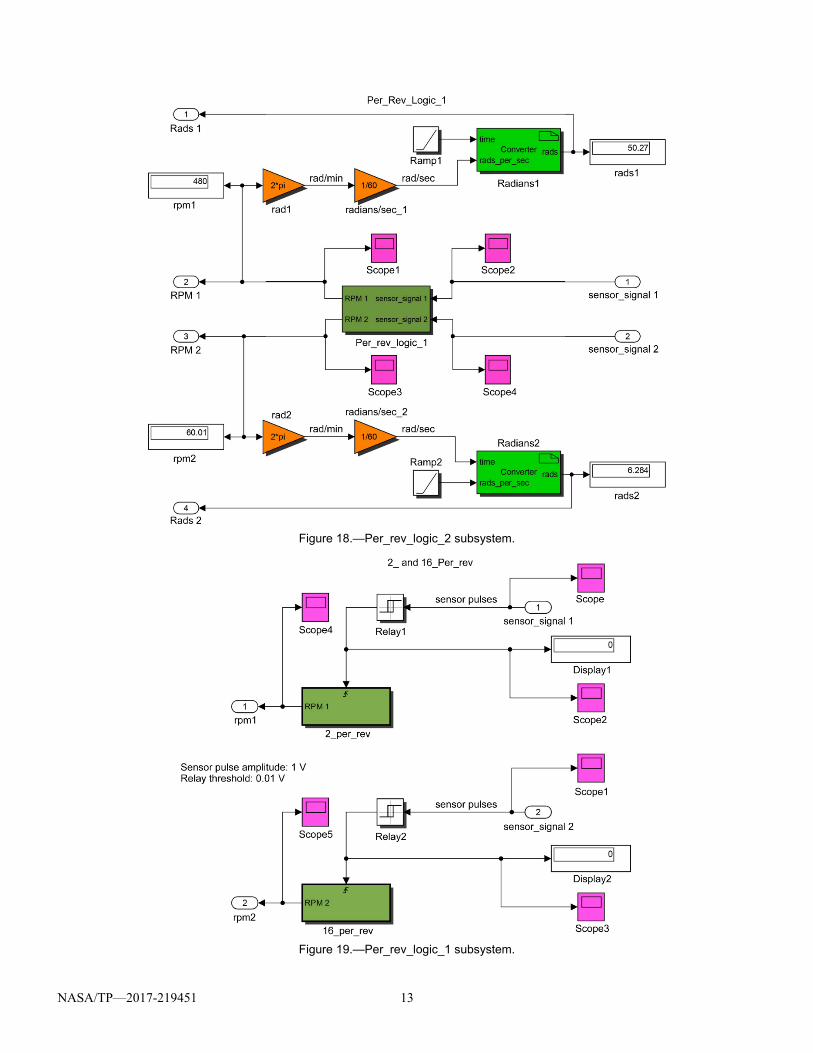
This section describes the features of the “Per_Rev_Logic” block. The “Per_Rev_Logic” subsystems’ level progression is shown in Figures 16 to 19. Figure 19 depicts the “RPM” blocks “2_per_rev” and “16_per_rev.” These blocks contain the subsystem that converts the proximity probe pulses, generated by the rotor’s notches, to the corresponding rotor rotational frequency. The subsystems are structured in this order, from top to bottom:

“Per_Rev_Logic”

○ “Per_Rev_Logic_3” – “Per_Rev_Logic_2”

“Per_Rev_Logic_1” 2_ and 16_Per_rev

Figure 16.—Per_rev_logic subsystem.

Figure 17.—Per_rev_logic_3 subsystem.

NASA/TP—2017-219451 13

Figure 18.—Per_rev_logic_2 subsystem.

Figure 19.—Per_rev_logic_1 subsystem.

NASA/TP—2017-219451 14

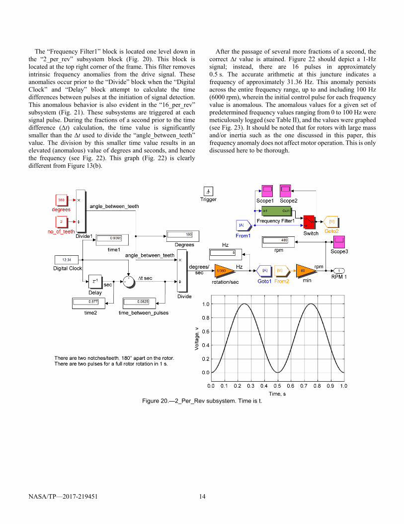
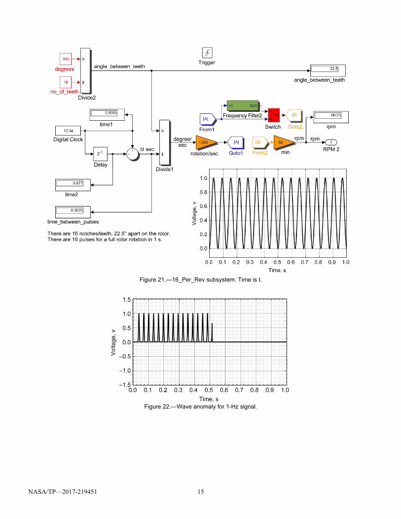
The “Frequency Filter1” block is located one level down in the “2_per_rev” subsystem block (Fig. 20). This block is located at the top right corner of the frame. This filter removes intrinsic frequency anomalies from the drive signal. These anomalies occur prior to the “Divide” block when the “Digital Clock” and “Delay” block attempt to calculate the time differences between pulses at the initiation of signal detection. This anomalous behavior is also evident in the “16_per_rev” subsystem (Fig. 21). These subsystems are triggered at each signal pulse. During the fractions of a second prior to the time difference (∆t) calculation, the time value is significantly smaller than the ∆t used to divide the “angle_between_teeth” value. The division by this smaller time value results in an elevated (anomalous) value of degrees and seconds, and hence the frequency (see Fig. 22). This graph (Fig. 22) is clearly different from Figure 13(b).

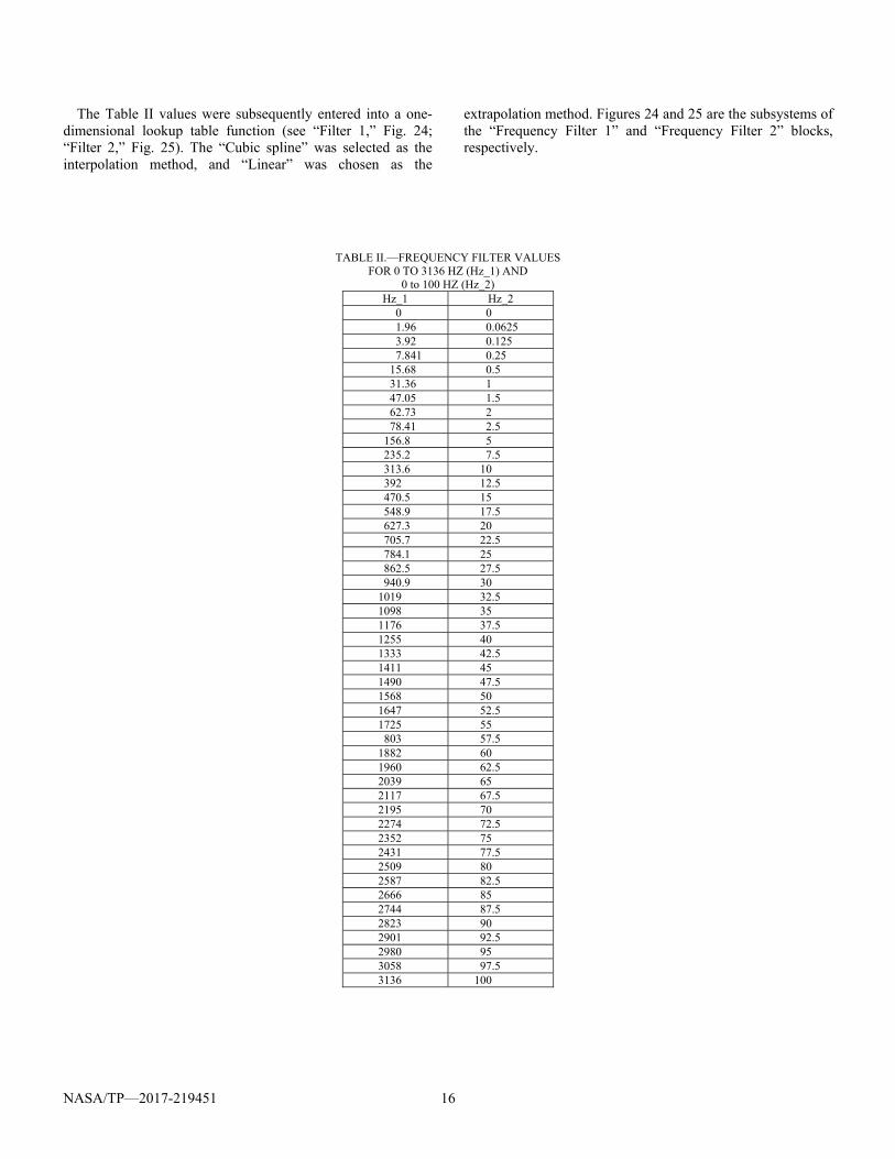
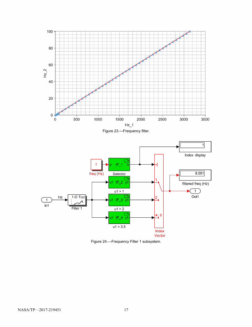
After the passage of several more fractions of a second, the correct ∆t value is attained. Figure 22 should depict a 1-Hz signal; instead, there are 16 pulses in approximately 0.5 s. The accurate arithmetic at this juncture indicates a frequency of approximately 31.36 Hz. This anomaly persists across the entire frequency range, up to and including 100 Hz (6000 rpm), wherein the initial control pulse for each frequency value is anomalous. The anomalous values for a given set of predetermined frequency values ranging from 0 to 100 Hz were meticulously logged (see Table II), and the values were graphed (see Fig. 23). It should be noted that for rotors with large mass and/or inertia such as the one discussed in this paper, this frequency anomaly does not affect motor operation. This is only discussed here to be thorough.

Figure 20.—2_Per_Rev subsystem. Time is t.

NASA/TP—2017-219451 15

Figure 21.—16_Per_Rev subsystem. Time is t.

Figure 22.—Wave anomaly for 1-Hz signal.

NASA/TP—2017-219451 16

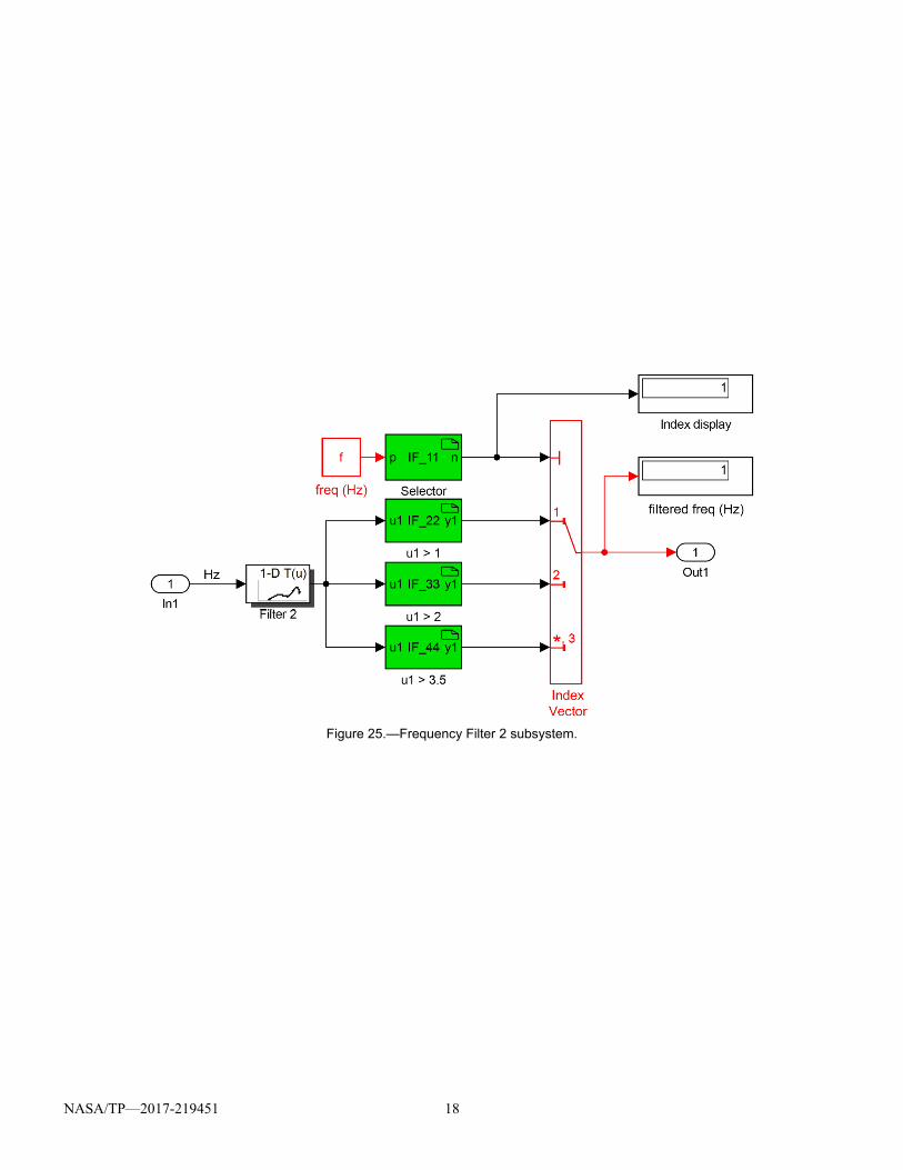
The Table II values were subsequently entered into a one-dimensional lookup table function (see “Filter 1,” Fig. 24; “Filter 2,” Fig. 25). The “Cubic spline” was selected as the interpolation method, and “Linear” was chosen as the

extrapolation method. Figures 24 and 25 are the subsystems of the “Frequency Filter 1” and “Frequency Filter 2” blocks, respectively.

TABLE II.—FREQUENCY FILTER VALUES FOR 0 TO 3136 HZ (Hz_1) AND

0 to 100 HZ (Hz_2) Hz_1 Hz_2

0 0 1.96 0.0625 3.92 0.125 7.841 0.25

15.68 0.5 31.36 1 47.05 1.5 62.73 2 78.41 2.5

156.8 5 235.2 7.5 313.6 10 392 12.5 470.5 15 548.9 17.5 627.3 20 705.7 22.5 784.1 25 862.5 27.5 940.9 30

1019 32.5 1098 35 1176 37.5 1255 40 1333 42.5 1411 45 1490 47.5 1568 50 1647 52.5 1725 55

803 57.5 1882 60 1960 62.5 2039 65 2117 67.5 2195 70 2274 72.5 2352 75 2431 77.5 2509 80 2587 82.5 2666 85 2744 87.5 2823 90 2901 92.5 2980 95 3058 97.5 3136 100

NASA/TP—2017-219451 17

Figure 23.—Frequency filter.

Figure 24.—Frequency Filter 1 subsystem.

NASA/TP—2017-219451 18

Figure 25.—Frequency Filter 2 subsystem.

NASA/TP—2017-219451 19

Phi_Angle_Controller

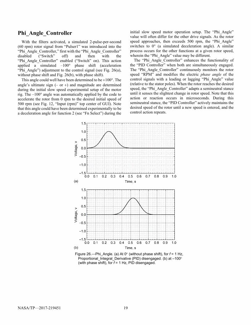
With the filters activated, a simulated 2-pulse-per-second (60 rpm) rotor signal from “Pulser1” was introduced into the “Phi_Angle_Controller,” first with the “Phi_Angle_Controller” disabled (“Switch” off) and then with the “Phi_Angle_Controller” enabled (“Switch” on). This action applied a simulated –100° phase shift (acceleration “Phi_Angle”) adjustment to the control signal (see Fig. 26(a), without phase shift and Fig. 26(b), with phase shift).

This angle could well have been determined to be 100°. The angle’s ultimate sign (– or ) and magnitude are determined during the initial slow speed experimental setup of the motor rig. The –100° angle was automatically applied by the code to accelerate the rotor from 0 rpm to the desired initial speed of 500 rpm (see Fig. 12, “Input (rpm)” top center of GUI). Note that this angle could have been determined experimentally to be a deceleration angle for function 2 (see “Fn Select”) during the

initial slow speed motor operation setup. The “Phi_Angle” value will often differ for the other drive signals. As the rotor speed approaches, then exceeds 500 rpm, the “Phi_Angle” switches to 0° (a simulated deceleration angle). A similar process occurs for the other functions at a given rotor speed, wherein the “Phi_Angle” value may be different.

The “Phi_Angle_Controller” enhances the functionality of the “PID Controller” when both are simultaneously engaged. The “Phi_Angle_Controller” continuously monitors the rotor speed “RPM” and modifies the electric phase angle of the control signals with a leading or lagging “Phi_Angle” value (relative to the stator poles). When the rotor reaches the desired speed, the “Phi_Angle_Controller” adapts a semineutral stance until it senses the slightest change in rotor speed. Note that this action or reaction occurs in microseconds. During this semineutral stance, the “PID Controller” actively maintains the desired speed of the rotor until a new speed is entered, and the control action repeats.

Figure 26.—Phi_Angle. (a) At 0 (without phase shift), for f = 1 Hz,

Proportional_Integral_Derivative (PID) disengaged. (b) at –100 (with phase shift), for f = 1 Hz, PID disengaged.

NASA/TP—2017-219451 20

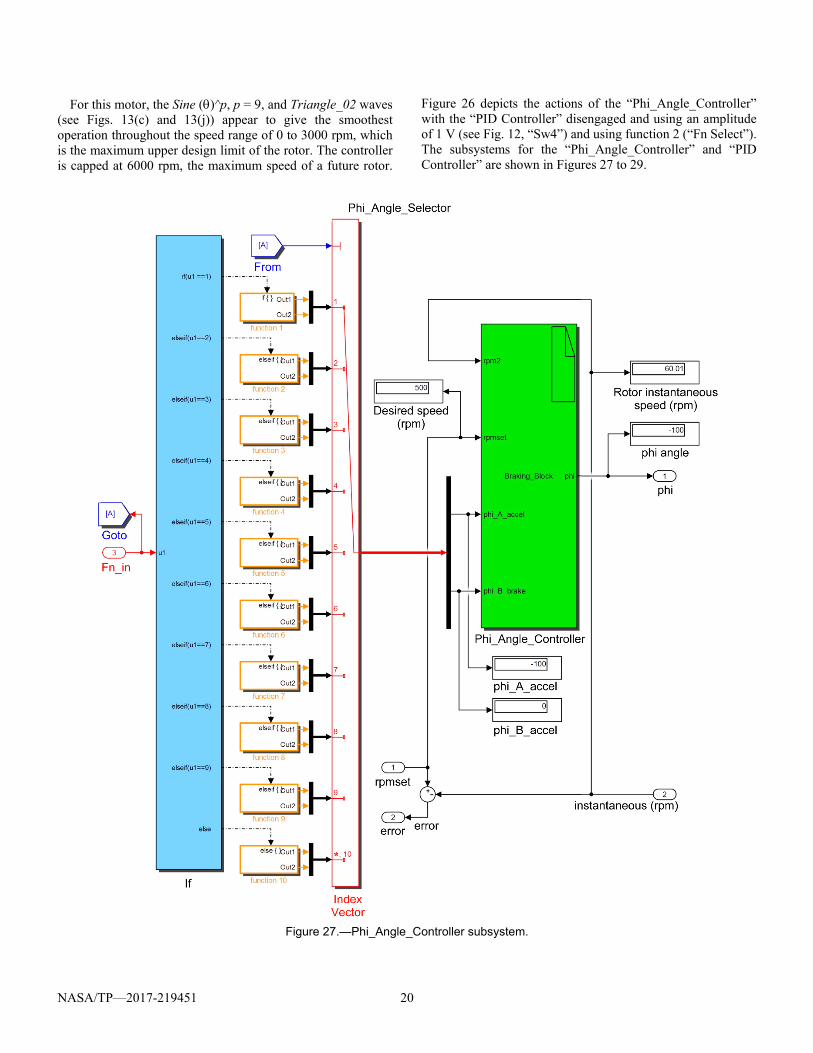
For this motor, the Sine ()^p, p = 9, and Triangle_02 waves (see Figs. 13(c) and 13(j)) appear to give the smoothest operation throughout the speed range of 0 to 3000 rpm, which is the maximum upper design limit of the rotor. The controller is capped at 6000 rpm, the maximum speed of a future rotor.

Figure 26 depicts the actions of the “Phi_Angle_Controller” with the “PID Controller” disengaged and using an amplitude of 1 V (see Fig. 12, “Sw4”) and using function 2 (“Fn Select”). The subsystems for the “Phi_Angle_Controller” and “PID Controller” are shown in Figures 27 to 29.

Figure 27.—Phi_Angle_Controller subsystem.

NASA/TP—2017-219451 21

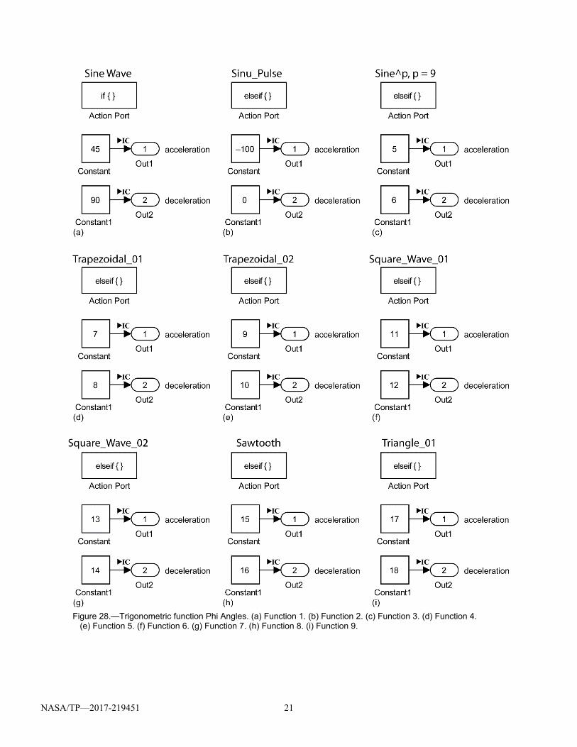
Figure 28.—Trigonometric function Phi Angles. (a) Function 1. (b) Function 2. (c) Function 3. (d) Function 4.

(e) Function 5. (f) Function 6. (g) Function 7. (h) Function 8. (i) Function 9.

NASA/TP—2017-219451 22

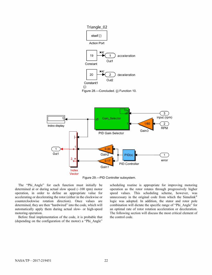
Figure 28.—Concluded. (j) Function 10.

Figure 29.—PID Controller subsystem.

The “Phi_Angle” for each function must initially be

determined at or during actual slow speed (~100 rpm) motor operation, in order to define an appropriate value for accelerating or decelerating the rotor (either in the clockwise or counterclockwise rotation direction). Once values are determined, they are then “hardwired” into the code, which will automatically apply them during actual slow- or high-speed motoring operation.

Before final implementation of the code, it is probable that (depending on the configuration of the motor) a “Phi_Angle”

scheduling routine is appropriate for improving motoring operation as the rotor rotates through progressively higher speed values. This scheduling scheme, however, was unnecessary in the original code from which the Simulink® logic was adopted. In addition, the stator and rotor pole combination will dictate the specific range of “Phi_Angle” for an optimal rate of rotor rotation acceleration or deceleration. The following section will discuss the most critical element of the control code.

NASA/TP—2017-219451 23

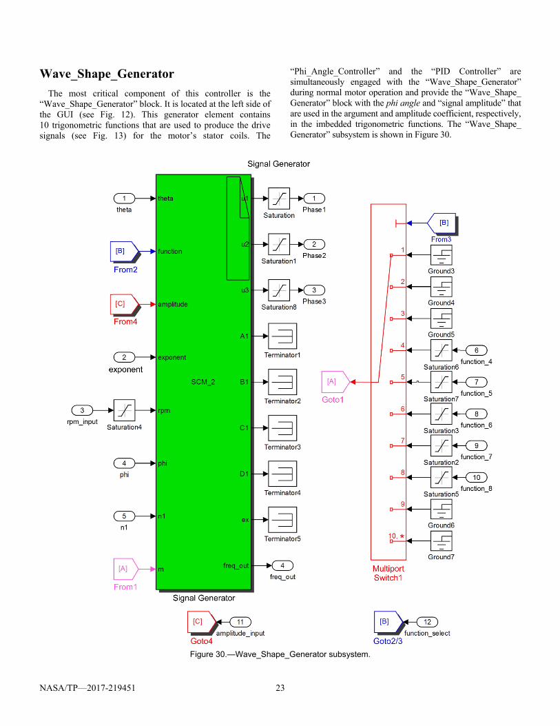
Wave_Shape_Generator

The most critical component of this controller is the “Wave_Shape_Generator” block. It is located at the left side of the GUI (see Fig. 12). This generator element contains 10 trigonometric functions that are used to produce the drive signals (see Fig. 13) for the motor’s stator coils. The

“Phi_Angle_Controller” and the “PID Controller” are simultaneously engaged with the “Wave_Shape_Generator” during normal motor operation and provide the “Wave_Shape_ Generator” block with the phi angle and “signal amplitude” that are used in the argument and amplitude coefficient, respectively, in the imbedded trigonometric functions. The “Wave_Shape_ Generator” subsystem is shown in Figure 30.

Figure 30.—Wave_Shape_Generator subsystem.

NASA/TP—2017-219451 24

On the left side of the “Wave_Shape_Generator” (see Fig. 12) there are a number of input ports. The input ports’ functions, from top to bottom, are as follows:

The “theta” port accepts “radians per second values”

from the “Per_Rev_Logic” block. The “exponent” port accepts constant values for the

exponent of the Sinu_Pulse, and Sine functions. The “rpm_input” port accepts the desired input rpm

values from the “Input (rpm)” block (see top center of GUI).

The “phi” port accepts “Phi_Angle_Controller” values for phi angle adjustment to the phase angle values.

The “n1” port accepts values for the maximum number of terms in the Fourier series representation for the following functions: o Trapezoidal_01 o Trapezoidal_02 o Square_Wave_01 o Square_Wave_02 o Sawtooth o Triangle_02

The “function_4” to “function_7” ports accepts values to adjust the pulse width of the following functions: o Trapezoidal_01 o Trapezoidal_02 o Square_Wave_01 o Square_Wave_02

The “function_8” port is unused at this time. The “amplitude_input” accepts constant or varying

amplitude values from the “PID Controller” depending on “Sw4” settings.

The “function_select” accepts values for selecting any of the 10 trigonometric function of the “Wave_Shape_Generator.”

The output ports “Phase1”, “Phase2”, “Phase3”, and

“freq_out” are on the right side of the “Wave_Shape_ Generator.” Output ports “Phase1” to “Phase3” provide the control signals that are ported to the dSPACE hardware which, in turn, is used to operate the motor. The motor’s rotor provides the pulses that are used in place of “Pulser1” or “Pulser2.”

NASA/TP—2017-219451 25

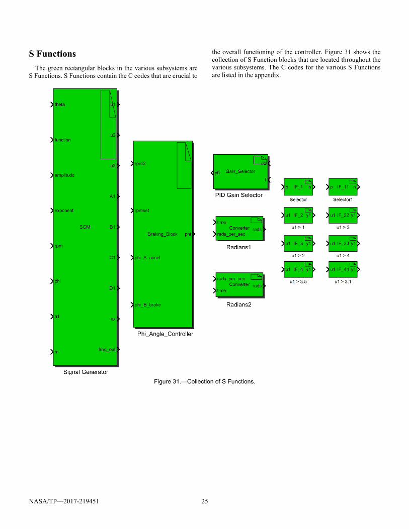
S Functions

The green rectangular blocks in the various subsystems are S Functions. S Functions contain the C codes that are crucial to

the overall functioning of the controller. Figure 31 shows the collection of S Function blocks that are located throughout the various subsystems. The C codes for the various S Functions are listed in the appendix.

Figure 31.—Collection of S Functions.

NASA/TP—2017-219451 26

Concluding Remarks

The MathWorks® Simulink® controller logic was adapted from an original C controller that successfully drove a room temperature, 36-tooth, four-pole, rotor reluctance motor. The C logic achieved a required rotor speed of 3000 rpm—the design limit of the rotor. The frequency filter in the Simulink® controller provided a more accurate input and output signal to the rotor by suppressing intrinsic signal anomalies, which were determined to be insignificant for high-inertial rotor operation. The Simulink® controller is versatile, and with slight modifications, can be used to drive other reluctance motor types incorporating dissimilar stator and rotor pole combinations. The controller was designed with the goal (after appropriate modification) of controlling a future superconducting motor that will be used as a testbed in the development of other

superconducting aviation propulsion motors envisioned for future turboelectric aircraft. The Simulink® findings presented in this report only apply in the simulated test environment. However, the simulated inputs would be replaced by actual proximity probe signals in a real-world dSPACE GmbH application. Safe and effective application of this code necessitates familiarity with the Simulink® and dSPACE technologies. It is advised that thorough simulation precede actual implementation and application of the code to familiarize the operator with its various control options, to prevent any unintentional code settings.

Glenn Research Center National Aeronautics and Space Administration Cleveland, Ohio, May 17, 2017

NASA/TP—2017-219451 27

Appendix

This appendix contains the signal generator functions. The appendix also contains the C programming code for the following—signal generator logic, phi angle controller, PID gain selector, radians 1 and 2, and frequency filter 1 and 2.

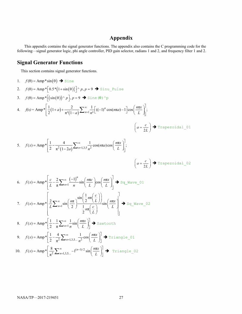
Signal Generator Functions

This section contains signal generator functions. 1. (θ) Amp*sinf Sine

2. (θ) Amp * 0.5* 1 sin ^ , 9f p p Sinu_Pulse

3. (θ) Amp * sin ^ , 9f p p Sine()^p

4. 1

1 2 1 π = Amp* 1 (( 1) cos( π ) 1 cos ;

2 π² 1 ²n

n

n xf(x) a n a

a n L

2

ca

L

Trapezoidal_01

5. 2 21,3,5

1 4 1 π( ) Amp* cos( π )cos ;

2 π 1 2 n

n xf x n a

La n

2

ca

L

Trapezoidal_02

6.

1

12 π π( ) Amp* sin cos

π

n

n

c n c n xf x

L n L L

Sq_Wave_01

7. 1

1sin π

22 π π( ) Amp* sin sin

12π

2

n

cn

Ln n xf x

cL Ln

L

Sq_Wave_02

8. 1

1 1 1 π( ) Amp* sin

2 π n

n xf x

n L

Sawtooth

9. 2 21,3,5

1 4 1 π( ) Amp* cos

2 π n

n xf x

Ln

Triangle_01

10. ( 1)/22 1,3,5

8 π( ) Amp* 1 sin

πn

n

n xf x

L

Triangle_02

NASA/TP—2017-219451 28

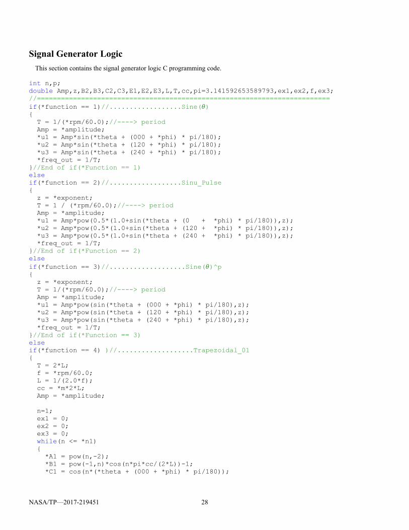
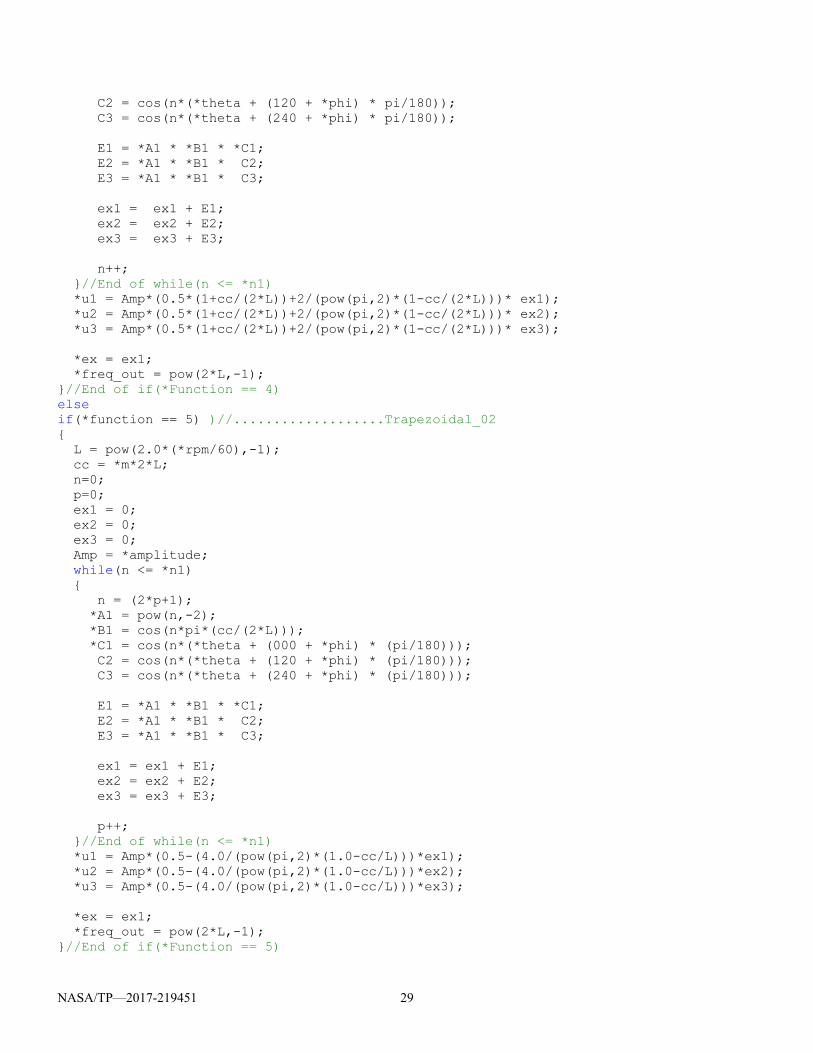
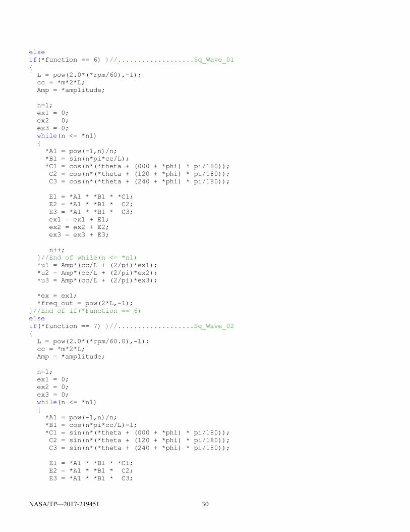
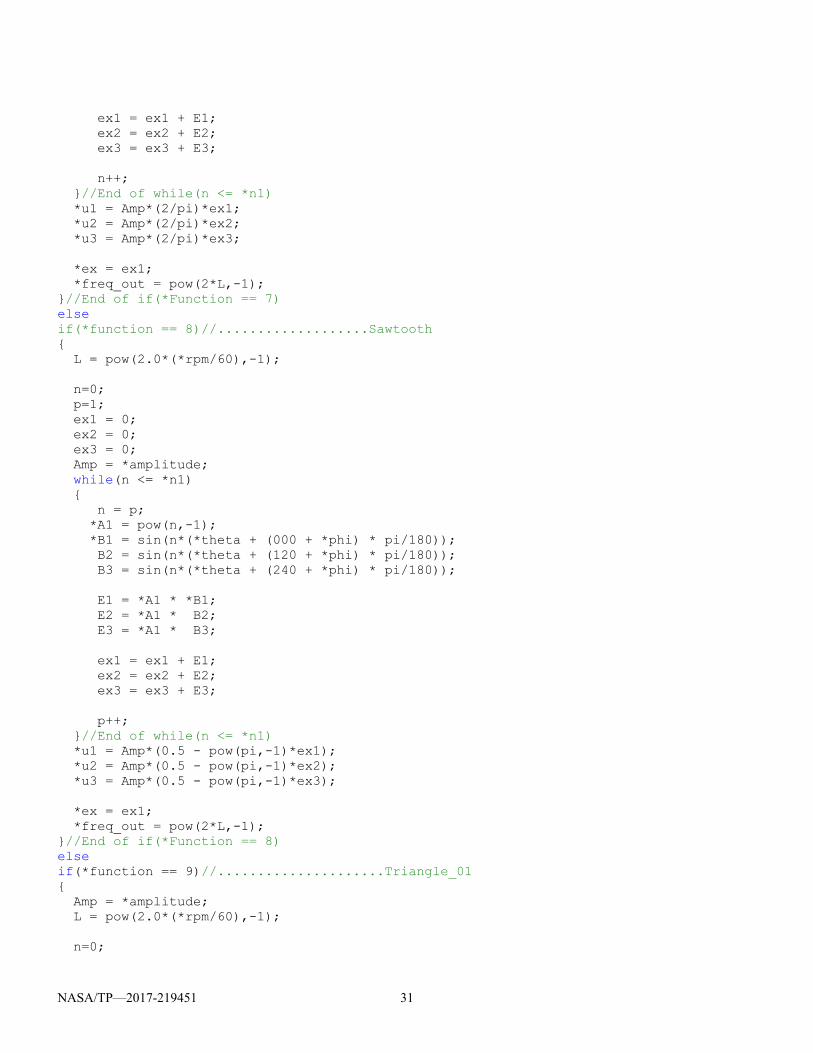
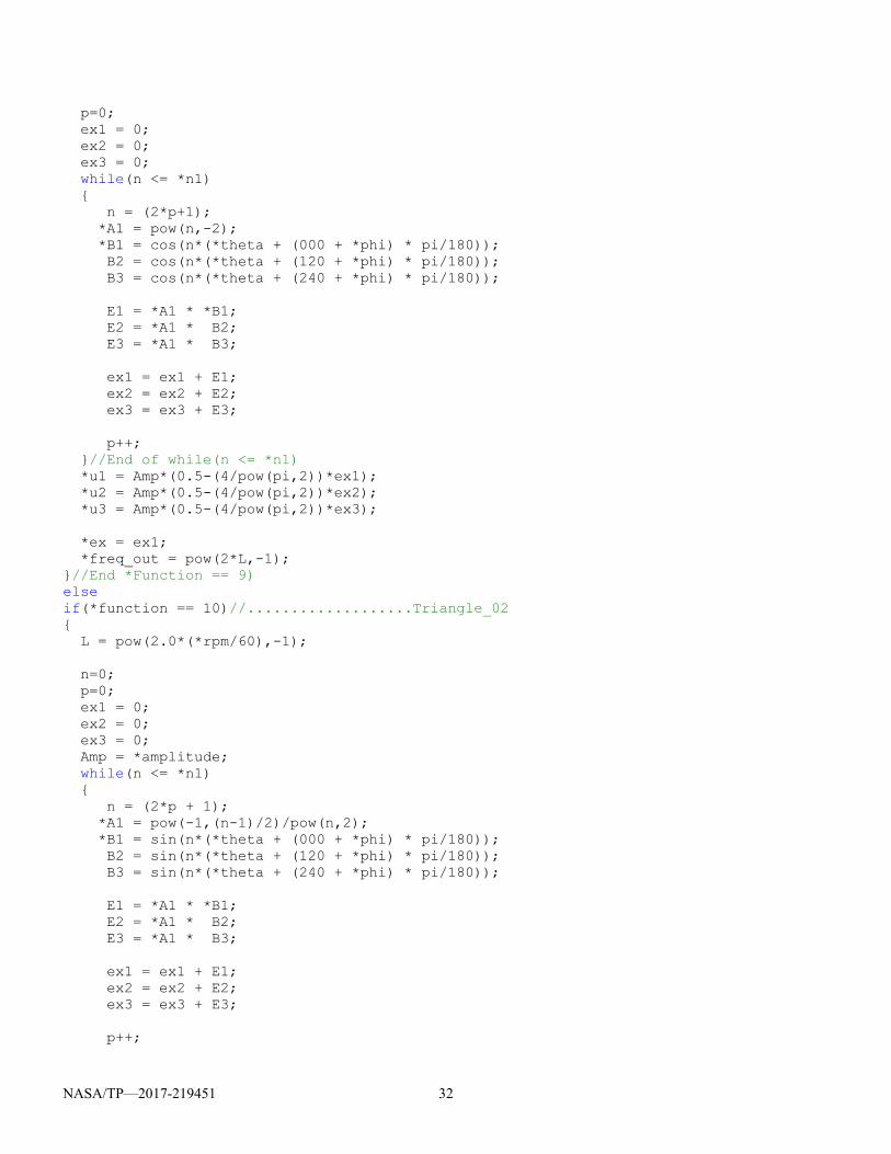
Signal Generator Logic

This section contains the signal generator logic C programming code.

int n,p; double Amp,z,B2,B3,C2,C3,E1,E2,E3,L,T,cc,pi=3.141592653589793,ex1,ex2,f,ex3; //========================================================================= if(*function == 1)//..................Sine( ) { T = 1/(*rpm/60.0);//----> period Amp = *amplitude; *u1 = Amp*sin(*theta + (000 + *phi) * pi/180); *u2 = Amp*sin(*theta + (120 + *phi) * pi/180); *u3 = Amp*sin(*theta + (240 + *phi) * pi/180); *freq_out = 1/T; }//End of if(*Function == 1) else if(*function == 2)//..................Sinu_Pulse { z = *exponent; T = 1 / (*rpm/60.0);//----> period Amp = *amplitude; *u1 = Amp*pow(0.5*(1.0+sin(*theta + (0 + *phi) * pi/180)),z); *u2 = Amp*pow(0.5*(1.0+sin(*theta + (120 + *phi) * pi/180)),z); *u3 = Amp*pow(0.5*(1.0+sin(*theta + (240 + *phi) * pi/180)),z); *freq_out = 1/T; }//End of if(*Function == 2) else if(*function == 3)//...................Sine( )^p { z = *exponent; T = 1/(*rpm/60.0);//----> period Amp = *amplitude; *u1 = Amp*pow(sin(*theta + (000 + *phi) * pi/180),z); *u2 = Amp*pow(sin(*theta + (120 + *phi) * pi/180),z); *u3 = Amp*pow(sin(*theta + (240 + *phi) * pi/180),z); *freq_out = 1/T; }//End of if(*Function == 3) else if(*function == 4) )//...................Trapezoidal_01 { T = 2*L; f = *rpm/60.0; L = 1/(2.0*f); cc = *m*2*L; Amp = *amplitude; n=1; ex1 = 0; ex2 = 0; ex3 = 0; while(n <= *n1) { *A1 = pow(n,-2); *B1 = pow(-1,n)*cos(n*pi*cc/(2*L))-1; *C1 = cos(n*(*theta + (000 + *phi) * pi/180));

NASA/TP—2017-219451 29

C2 = cos(n*(*theta + (120 + *phi) * pi/180)); C3 = cos(n*(*theta + (240 + *phi) * pi/180)); E1 = *A1 * *B1 * *C1; E2 = *A1 * *B1 * C2; E3 = *A1 * *B1 * C3; ex1 = ex1 + E1; ex2 = ex2 + E2; ex3 = ex3 + E3; n++; }//End of while(n <= *n1) *u1 = Amp*(0.5*(1+cc/(2*L))+2/(pow(pi,2)*(1-cc/(2*L)))* ex1); *u2 = Amp*(0.5*(1+cc/(2*L))+2/(pow(pi,2)*(1-cc/(2*L)))* ex2); *u3 = Amp*(0.5*(1+cc/(2*L))+2/(pow(pi,2)*(1-cc/(2*L)))* ex3); *ex = ex1; *freq_out = pow(2*L,-1); }//End of if(*Function == 4) else if(*function == 5) )//...................Trapezoidal_02 { L = pow(2.0*(*rpm/60),-1); cc = *m*2*L; n=0; p=0; ex1 = 0; ex2 = 0; ex3 = 0; Amp = *amplitude; while(n <= *n1) { n = (2*p+1); *A1 = pow(n,-2); *B1 = cos(n*pi*(cc/(2*L))); *C1 = cos(n*(*theta + (000 + *phi) * (pi/180))); C2 = cos(n*(*theta + (120 + *phi) * (pi/180))); C3 = cos(n*(*theta + (240 + *phi) * (pi/180))); E1 = *A1 * *B1 * *C1; E2 = *A1 * *B1 * C2; E3 = *A1 * *B1 * C3; ex1 = ex1 + E1; ex2 = ex2 + E2; ex3 = ex3 + E3; p++; }//End of while(n <= *n1) *u1 = Amp*(0.5-(4.0/(pow(pi,2)*(1.0-cc/L)))*ex1); *u2 = Amp*(0.5-(4.0/(pow(pi,2)*(1.0-cc/L)))*ex2); *u3 = Amp*(0.5-(4.0/(pow(pi,2)*(1.0-cc/L)))*ex3); *ex = ex1; *freq_out = pow(2*L,-1); }//End of if(*Function == 5)

NASA/TP—2017-219451 30

else if(*function == 6) )//...................Sq_Wave_01 { L = pow(2.0*(*rpm/60),-1); cc = *m*2*L; Amp = *amplitude; n=1; ex1 = 0; ex2 = 0; ex3 = 0; while(n <= *n1) { *A1 = pow(-1,n)/n; *B1 = sin(n*pi*cc/L); *C1 = cos(n*(*theta + (000 + *phi) * pi/180)); C2 = cos(n*(*theta + (120 + *phi) * pi/180)); C3 = cos(n*(*theta + (240 + *phi) * pi/180)); E1 = *A1 * *B1 * *C1; E2 = *A1 * *B1 * C2; E3 = *A1 * *B1 * C3; ex1 = ex1 + E1; ex2 = ex2 + E2; ex3 = ex3 + E3; n++; }//End of while(n <= *n1) *u1 = Amp*(cc/L + (2/pi)*ex1); *u2 = Amp*(cc/L + (2/pi)*ex2); *u3 = Amp*(cc/L + (2/pi)*ex3); *ex = ex1; *freq_out = pow(2*L,-1); }//End of if(*Function == 6) else if(*function == 7) )//...................Sq_Wave_02 { L = pow(2.0*(*rpm/60.0),-1); cc = *m*2*L; Amp = *amplitude; n=1; ex1 = 0; ex2 = 0; ex3 = 0; while(n <= *n1) { *A1 = pow(-1,n)/n; *B1 = cos(n*pi*cc/L)-1; *C1 = sin(n*(*theta + (000 + *phi) * pi/180)); C2 = sin(n*(*theta + (120 + *phi) * pi/180)); C3 = sin(n*(*theta + (240 + *phi) * pi/180)); E1 = *A1 * *B1 * *C1; E2 = *A1 * *B1 * C2; E3 = *A1 * *B1 * C3;

NASA/TP—2017-219451 31

ex1 = ex1 + E1; ex2 = ex2 + E2; ex3 = ex3 + E3; n++; }//End of while(n <= *n1) *u1 = Amp*(2/pi)*ex1; *u2 = Amp*(2/pi)*ex2; *u3 = Amp*(2/pi)*ex3; *ex = ex1; *freq_out = pow(2*L,-1); }//End of if(*Function == 7) else if(*function == 8)//...................Sawtooth { L = pow(2.0*(*rpm/60),-1); n=0; p=1; ex1 = 0; ex2 = 0; ex3 = 0; Amp = *amplitude; while(n <= *n1) { n = p; *A1 = pow(n,-1); *B1 = sin(n*(*theta + (000 + *phi) * pi/180)); B2 = sin(n*(*theta + (120 + *phi) * pi/180)); B3 = sin(n*(*theta + (240 + *phi) * pi/180)); E1 = *A1 * *B1; E2 = *A1 * B2; E3 = *A1 * B3; ex1 = ex1 + E1; ex2 = ex2 + E2; ex3 = ex3 + E3; p++; }//End of while(n <= *n1) *u1 = Amp*(0.5 - pow(pi,-1)*ex1); *u2 = Amp*(0.5 - pow(pi,-1)*ex2); *u3 = Amp*(0.5 - pow(pi,-1)*ex3); *ex = ex1; *freq_out = pow(2*L,-1); }//End of if(*Function == 8) else if(*function == 9)//.....................Triangle_01 { Amp = *amplitude; L = pow(2.0*(*rpm/60),-1); n=0;

NASA/TP—2017-219451 32

p=0; ex1 = 0; ex2 = 0; ex3 = 0; while(n <= *n1) { n = (2*p+1); *A1 = pow(n,-2); *B1 = cos(n*(*theta + (000 + *phi) * pi/180)); B2 = cos(n*(*theta + (120 + *phi) * pi/180)); B3 = cos(n*(*theta + (240 + *phi) * pi/180)); E1 = *A1 * *B1; E2 = *A1 * B2; E3 = *A1 * B3; ex1 = ex1 + E1; ex2 = ex2 + E2; ex3 = ex3 + E3; p++; }//End of while(n <= *n1) *u1 = Amp*(0.5-(4/pow(pi,2))*ex1); *u2 = Amp*(0.5-(4/pow(pi,2))*ex2); *u3 = Amp*(0.5-(4/pow(pi,2))*ex3); *ex = ex1; *freq_out = pow(2*L,-1); }//End *Function == 9) else if(*function == 10)//...................Triangle_02 { L = pow(2.0*(*rpm/60),-1); n=0; p=0; ex1 = 0; ex2 = 0; ex3 = 0; Amp = *amplitude; while(n <= *n1) { n = (2*p + 1); *A1 = pow(-1,(n-1)/2)/pow(n,2); *B1 = sin(n*(*theta + (000 + *phi) * pi/180)); B2 = sin(n*(*theta + (120 + *phi) * pi/180)); B3 = sin(n*(*theta + (240 + *phi) * pi/180)); E1 = *A1 * *B1; E2 = *A1 * B2; E3 = *A1 * B3; ex1 = ex1 + E1; ex2 = ex2 + E2; ex3 = ex3 + E3; p++;

NASA/TP—2017-219451 33

}//End of while(n <= *n1) *u1 = Amp*(8/pow(pi,2))*ex1; *u2 = Amp*(8/pow(pi,2))*ex2; *u3 = Amp*(8/pow(pi,2))*ex3; *ex = ex1; *freq_out = pow(2*L,-1); }//End of if(*Function == 10)

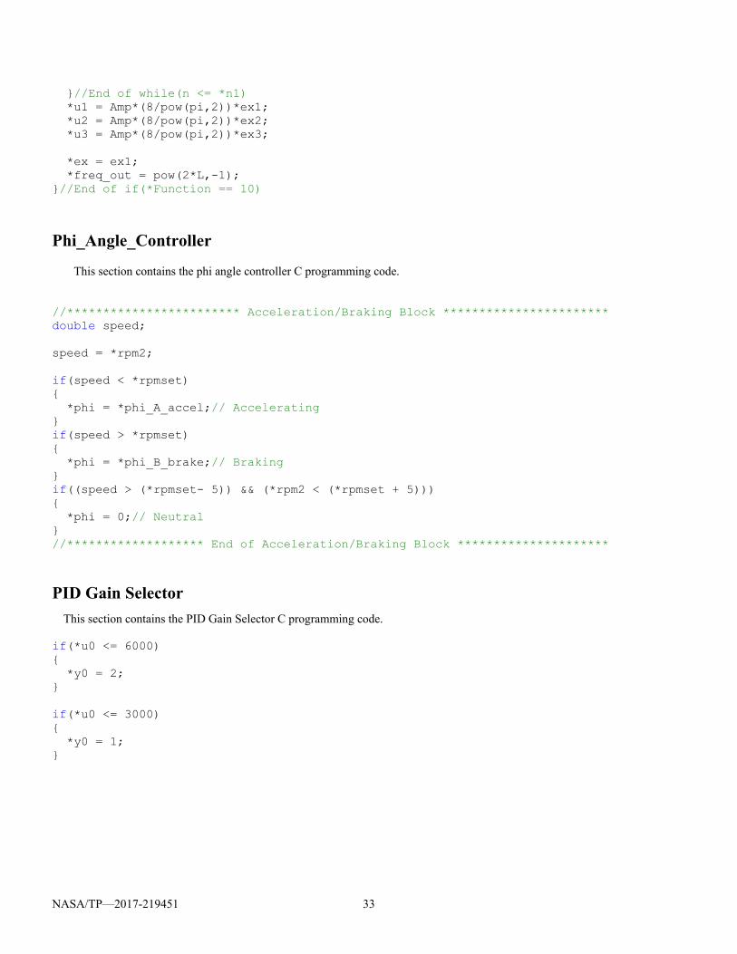
Phi_Angle_Controller

This section contains the phi angle controller C programming code. //************************ Acceleration/Braking Block *********************** double speed; speed = *rpm2; if(speed < *rpmset) { *phi = *phi_A_accel;// Accelerating } if(speed > *rpmset) { *phi = *phi_B_brake;// Braking } if((speed > (*rpmset- 5)) && (*rpm2 < (*rpmset + 5))) { *phi = 0;// Neutral } //******************* End of Acceleration/Braking Block *********************

PID Gain Selector

This section contains the PID Gain Selector C programming code.

if(*u0 <= 6000) { *y0 = 2; } if(*u0 <= 3000) { *y0 = 1; }

NASA/TP—2017-219451 34

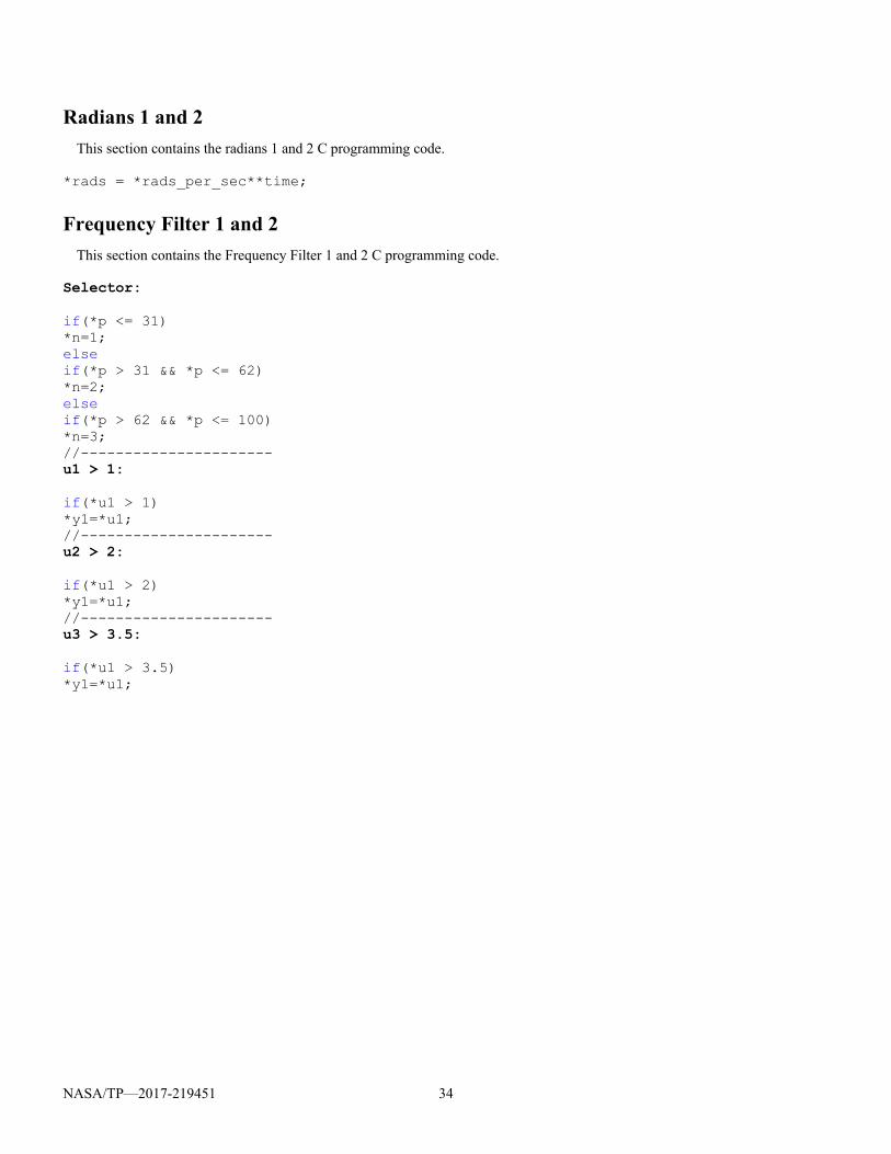
Radians 1 and 2

This section contains the radians 1 and 2 C programming code.

*rads = *rads_per_sec**time;

Frequency Filter 1 and 2

This section contains the Frequency Filter 1 and 2 C programming code. Selector: if(*p <= 31) *n=1; else if(*p > 31 && *p <= 62) *n=2; else if(*p > 62 && *p <= 100) *n=3; //---------------------- u1 > 1: if(*u1 > 1) *y1=*u1; //---------------------- u2 > 2: if(*u1 > 2) *y1=*u1; //---------------------- u3 > 3.5: if(*u1 > 3.5) *y1=*u1;

NASA/TP—2017-219451 35

Bibliography

Zamboni, Luca: Getting Started with Simulink, Packt Publishing Ltd., Birmingham, England, 2013.

Dabney, James B.; and Harman, Thomas L.: Mastering Simulink. Prentice Hall, Upper Saddle River, NJ, 2004.

Allain, Alex: Jumping Into C++. Cprogramming.com, San Francisco, CA, 2012.

Horton, Ivor: Ivor Horton’s Beginning Visual C++ 2012. John Wiley & Sons, Indianapolis, IN, 2012.

Morrison, Carlos R.: Bearingless Switched Reluctance Motor. U.S. Patent no. 6,727,618 B1, 2004.

References

1. Morrison, Carlos. R; Ho, Eric J.; and Siebert, Mark W.: Electromagnetic Forces in a Hybrid Magnetic-Bearing Switched-Reluctance Motor. NASA/TP—2008-214818, 2008. http://ntrs.nasa.gov