Simultaneous Tracking and Estimation of a Skeletal Model

Simultaneous Tracking and Estimation of a Skeletal Model forMonitoring Human Motion

Stephane Drouin, Patrick Hebert and Marc ParizeauComputer Vision and Systems Laboratory

Department of Electrical and Computer EngineeringLaval University, Sainte-Foy, QC, Canada, G1K 7P4

{sdrouin, hebert, parizeau}@gel.ulaval.ca

Abstract

This paper presents a vision system for tracking a 3Darticulated human model from the observation of isolatedfeatures from multiple viewpoints. A generic model is in-stantiated by estimating invariant elements (limb lengths)during tracking. The model is used as feedback both inthe estimation module for filtering and in the segmenta-tion module where it predicts the feature’s position andsize. Filtering is carried out with a Kalman filter withimproved numerical stability using Joseph’s implemen-tation. The robustness of this implementation is com-pared to the basic formulation on real sequences. Resultsdemonstrate a rapid convergence of the filtered parame-ters despite large observation variances.

1 Introduction

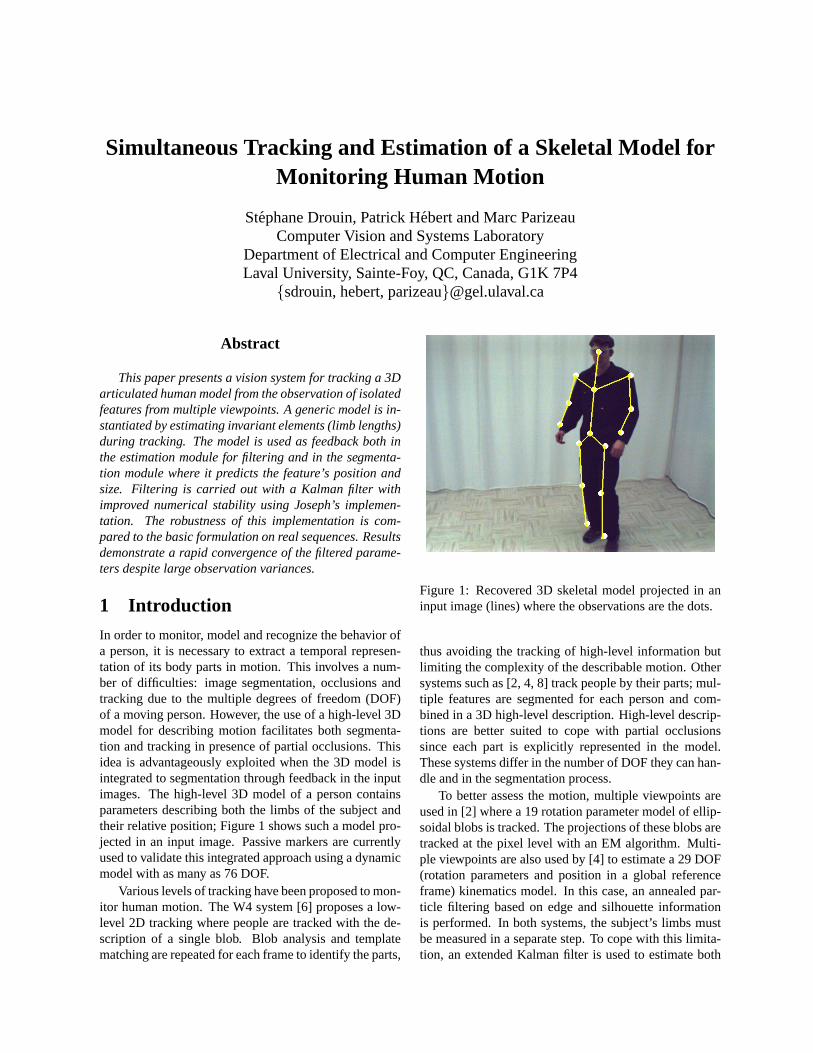
In order to monitor, model and recognize the behavior ofa person, it is necessary to extract a temporal represen-tation of its body parts in motion. This involves a num-ber of difficulties: image segmentation, occlusions andtracking due to the multiple degrees of freedom (DOF)of a moving person. However, the use of a high-level 3Dmodel for describing motion facilitates both segmenta-tion and tracking in presence of partial occlusions. Thisidea is advantageously exploited when the 3D model isintegrated to segmentation through feedback in the inputimages. The high-level 3D model of a person containsparameters describing both the limbs of the subject andtheir relative position; Figure 1 shows such a model pro-jected in an input image. Passive markers are currentlyused to validate this integrated approach using a dynamicmodel with as many as 76 DOF.

Various levels of tracking have been proposed to mon-itor human motion. The W4 system [6] proposes a low-level 2D tracking where people are tracked with the de-scription of a single blob. Blob analysis and templatematching are repeated for each frame to identify the parts,

Figure 1: Recovered 3D skeletal model projected in aninput image (lines) where the observations are the dots.

thus avoiding the tracking of high-level information butlimiting the complexity of the describable motion. Othersystems such as [2, 4, 8] track people by their parts; mul-tiple features are segmented for each person and com-bined in a 3D high-level description. High-level descrip-tions are better suited to cope with partial occlusionssince each part is explicitly represented in the model.These systems differ in the number of DOF they can han-dle and in the segmentation process.

To better assess the motion, multiple viewpoints areused in [2] where a 19 rotation parameter model of ellip-soidal blobs is tracked. The projections of these blobs aretracked at the pixel level with an EM algorithm. Multi-ple viewpoints are also used by [4] to estimate a 29 DOF(rotation parameters and position in a global referenceframe) kinematics model. In this case, an annealed par-ticle filtering based on edge and silhouette informationis performed. In both systems, the subject’s limbs mustbe measured in a separate step. To cope with this limita-tion, an extended Kalman filter is used to estimate both

Drouin & al., Vision Interface 2003 2

rotation parameters and limb lengths in [8]. Neverthelessthe system only tracks a human arm with 3 DOF from asingle viewpoint.

This paper presents a closed-loop system related to[8] inasmuch as it uses feature points as input to an ex-tended Kalman filter and it simultaneously estimates limblength parameters. In our case, a 76 DOF model istracked from its projection in multiple viewpoints. Theincreased dimensionality introduces the need for numer-ically stable methods as well as increased robustness toocclusions. The extended Kalman filter is revisited toimprove numerical stability when combining the obser-vation of markers. Feedback from the predicted obser-vation in each image allows a segmentation procedure toextract and label feature points on the subject. The pro-cedure is robust to occlusions and to prolonged absenceof data.

The paper is organized as follows: Section 2 describesthe proposed system, Section 3 introduces the mathemat-ical models used for tracking and results are given in Sec-tion 4.

2 System overviewThe tracked model is shown in Figure 1; its 76 DOF in-clude length, angle, position and velocity parameters todescribe the subject and its motion. Four stages of pro-cessing are needed in order to produce a high-level de-scription of the actions of a person [7]: initialization,tracking, pose estimation and recognition. In the initial-ization stage, it is necessary to instantiate a generic modelor to obtain the first segmentation. Tracking consists insegmenting the subject and establishing a correspondencebetween the images. For a sequence of images, a timecorrespondence must be established for the features in asame viewpoint; with multiple cameras, a space corre-spondence must also be established between the view-points. Pose estimation consists in representing the rel-ative position of the body parts of the subject. Finally,recognition consists in providing a high-level descriptionto a sequence of images.

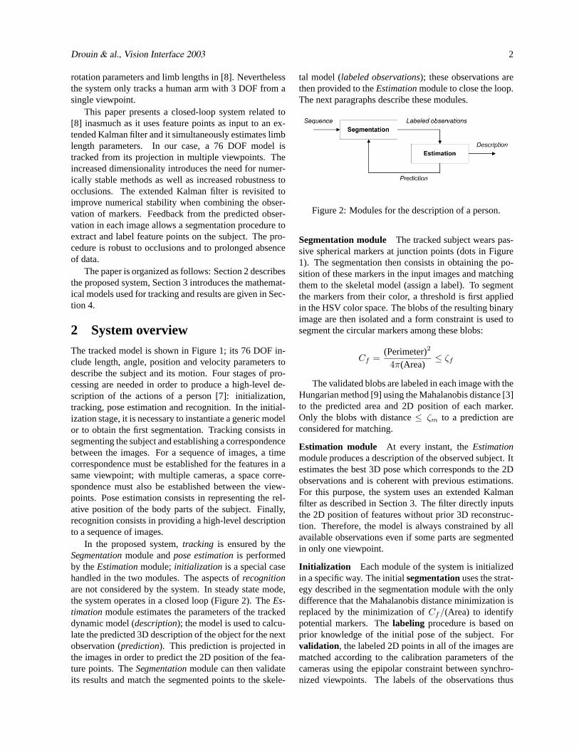
In the proposed system,tracking is ensured by theSegmentationmodule andpose estimationis performedby theEstimationmodule;initialization is a special casehandled in the two modules. The aspects ofrecognitionare not considered by the system. In steady state mode,the system operates in a closed loop (Figure 2). TheEs-timationmodule estimates the parameters of the trackeddynamic model (description); the model is used to calcu-late the predicted 3D description of the object for the nextobservation (prediction). This prediction is projected inthe images in order to predict the 2D position of the fea-ture points. TheSegmentationmodule can then validateits results and match the segmented points to the skele-

tal model (labeled observations); these observations arethen provided to theEstimationmodule to close the loop.The next paragraphs describe these modules.

Figure 2: Modules for the description of a person.

Segmentation module The tracked subject wears pas-sive spherical markers at junction points (dots in Figure1). The segmentation then consists in obtaining the po-sition of these markers in the input images and matchingthem to the skeletal model (assign a label). To segmentthe markers from their color, a threshold is first appliedin the HSV color space. The blobs of the resulting binaryimage are then isolated and a form constraint is used tosegment the circular markers among these blobs:

Cf =(Perimeter)2

4π(Area)≤ ζf

The validated blobs are labeled in each image with theHungarian method [9] using the Mahalanobis distance [3]to the predicted area and 2D position of each marker.Only the blobs with distance≤ ζm to a prediction areconsidered for matching.

Estimation module At every instant, theEstimationmodule produces a description of the observed subject. Itestimates the best 3D pose which corresponds to the 2Dobservations and is coherent with previous estimations.For this purpose, the system uses an extended Kalmanfilter as described in Section 3. The filter directly inputsthe 2D position of features without prior 3D reconstruc-tion. Therefore, the model is always constrained by allavailable observations even if some parts are segmentedin only one viewpoint.

Initialization Each module of the system is initializedin a specific way. The initialsegmentationuses the strat-egy described in the segmentation module with the onlydifference that the Mahalanobis distance minimization isreplaced by the minimization ofCf/(Area) to identifypotential markers. Thelabeling procedure is based onprior knowledge of the initial pose of the subject. Forvalidation, the labeled 2D points in all of the images arematched according to the calibration parameters of thecameras using the epipolar constraint between synchro-nized viewpoints. The labels of the observations thus


paired are compared; a voting procedure among the im-ages where each marker was segmented determines if alabel is to be validated (more than50% of the votes agree)or if the observations are invalidated (no majority). Assoon as all of the markers are correctly segmented andmatched, their 3D positions are calculated and the initialparameters of the model areestimated.

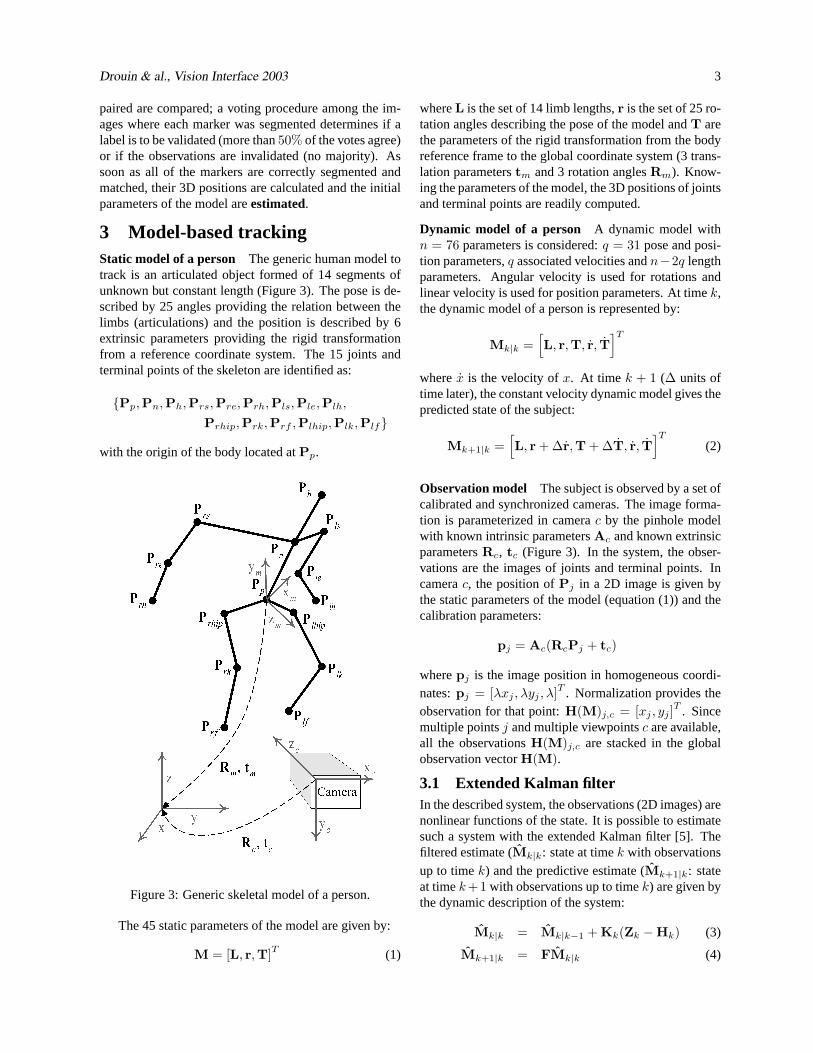
3 Model-based trackingStatic model of a person The generic human model totrack is an articulated object formed of 14 segments ofunknown but constant length (Figure 3). The pose is de-scribed by 25 angles providing the relation between thelimbs (articulations) and the position is described by 6extrinsic parameters providing the rigid transformationfrom a reference coordinate system. The 15 joints andterminal points of the skeleton are identified as:

{Pp,Pn,Ph,Prs,Pre,Prh,Pls,Ple,Plh,

Prhip,Prk,Prf ,Plhip,Plk,Plf}

with the origin of the body located atPp.

Figure 3: Generic skeletal model of a person.

The 45 static parameters of the model are given by:

M = [L, r,T]T (1)

whereL is the set of 14 limb lengths,r is the set of 25 ro-tation angles describing the pose of the model andT arethe parameters of the rigid transformation from the bodyreference frame to the global coordinate system (3 trans-lation parameterstm and 3 rotation anglesRm). Know-ing the parameters of the model, the 3D positions of jointsand terminal points are readily computed.

Dynamic model of a person A dynamic model withn = 76 parameters is considered:q = 31 pose and posi-tion parameters,q associated velocities andn−2q lengthparameters. Angular velocity is used for rotations andlinear velocity is used for position parameters. At timek,the dynamic model of a person is represented by:

Mk|k =[L, r,T, r, T

]T

wherex is the velocity ofx. At time k + 1 (∆ units oftime later), the constant velocity dynamic model gives thepredicted state of the subject:

Mk+1|k =[L, r + ∆r,T + ∆T, r, T

]T

(2)

Observation model The subject is observed by a set ofcalibrated and synchronized cameras. The image forma-tion is parameterized in camerac by the pinhole modelwith known intrinsic parametersAc and known extrinsicparametersRc, tc (Figure 3). In the system, the obser-vations are the images of joints and terminal points. Incamerac, the position ofPj in a 2D image is given bythe static parameters of the model (equation (1)) and thecalibration parameters:

pj = Ac(RcPj + tc)

wherepj is the image position in homogeneous coordi-nates:pj = [λxj , λyj , λ]T . Normalization provides theobservation for that point:H(M)j,c = [xj , yj ]

T . Sincemultiple pointsj and multiple viewpointsc are available,all the observationsH(M)j,c are stacked in the globalobservation vectorH(M).

3.1 Extended Kalman filterIn the described system, the observations (2D images) arenonlinear functions of the state. It is possible to estimatesuch a system with the extended Kalman filter [5]. Thefiltered estimate (Mk|k: state at timek with observationsup to timek) and the predictive estimate (Mk+1|k: stateat timek+1 with observations up to timek) are given bythe dynamic description of the system:

Mk|k = Mk|k−1 + Kk(Zk −Hk) (3)

Mk+1|k = FMk|k (4)


whereF is the dynamic matrix of the system,Hk ,H(Mk|k−1) is the (non-linear) prediction of the obser-vation,Zk is the observation andKk is the Kalman gain.From (2),

F = In + ∆

0n−2q,n−q 0n−2q,q

0q,n−q Iq

0q,n−q 0q,q

whereIn is then× n identity matrix and0q,q is aq × qnull matrix.

Kk = Σk|k−1hTk

(hkΣk|k−1hT

k + Rk

)−1(5)

wherehk , δH(M)δM |M=Mk|k−1

andRk is the covariancematrix of the observations (measurement error). The co-variance matrices of the filtered estimate (Σk|k) and thepredictive estimate (Σk|k−1) are given by:

Σk|k = (I−Kkhk)Σk|k−1 (6)

Σk|k−1 = FΣk−1|k−1FT + Qk−1 (7)

whereQk−1 is the covariance matrix of the system noise(model error).

Iterated Kalman filter The error caused by the lin-earization of the filter near the prediction can be de-creased using the iterated Kalman filter [1, 10]. It consistsin replacing the filtered estimate (3) and the Kalman gain(5) with their locally iterated versions (i = 0, 1, ..., I−1):

Mk|k,i+1 = Mk|k−1+

Kk,i

[Zk −Hk,i − hk,i(Mk|k−1 − Mk|k,i)

]

Kk,i = Σk|k−1hTk,i

(hk,iΣk|k−1hT

k,i + Rk

)−1

with the initialization Mk|k,0 = Mk|k−1 and where

Hk,i , H(Mk|k,i) andhk,i , δH(M)δM |M=Mk|k,i

. Thefiltered estimate and its covariance are then given by:

Mk|k = Mk|k,I

Σk|k = (I−Kk,Ihk,I)Σk|k−1

ChoosingI = 1 brings us back to the extended Kalmanfilter. An automatic stop criterion can be added: givenε(M) = ‖Zk −H(M)‖, iterate as long as the followingconditions are all true:

i < I,

ε(Mk|k,i+1) ≥ εE ,

ε(Mk|k,i)− ε(Mk|k,i+1) ≥ εD,

whereεE andεD are tolerances on observation error andobservation error improvement, respectively.

Joseph’s form equation The direct implementation ofthe Kalman equations gives rise to a numerically unstablefilter [5]. The covariance matrix of the filtered estimateis particularly sensitive to rounding errors since no feed-back makes it possible to correct the accumulated errors.Joseph’s form equation for the update of the covariancematrix has a better numerical stability than the basic im-plementation; it is given by:

Σk|k = (I−Kkhk)Σk|k−1 (I−Kkhk)T

+ KkRkKTk

Using (5), it is easily shown that Joseph’s form is equiv-alent to the basic equation (6) for the update of the co-variance [5]. Although it involves more computation,this form has the advantage of preserving the symmetryand positive definiteness of the covariance matrix despiterounding errors.

3.2 Initialization of the filterThe system must be initialized by providingM0 andΣ0.The initial static parameters of the model are calculatedfrom a first set of the 15 joint 3D positions and all ve-locities are initialized to 0.Σ0 must be initialized withrealistic values, with respect to the precision of the 3D re-construction and to modeling error caused by the choiceof initial velocities. For each image, the filter must alsobe provided with the value of the observation covarianceRk and the system noiseQk−1.

While the observation and initial state covariances canbe estimated experimentally, the system noise is difficultto evaluate. It must account for modeling error such asnon-constant velocity motion and non-rigid body parts.The values of the covariance matrices are manually set inthe experiments; they are given in Section 4.

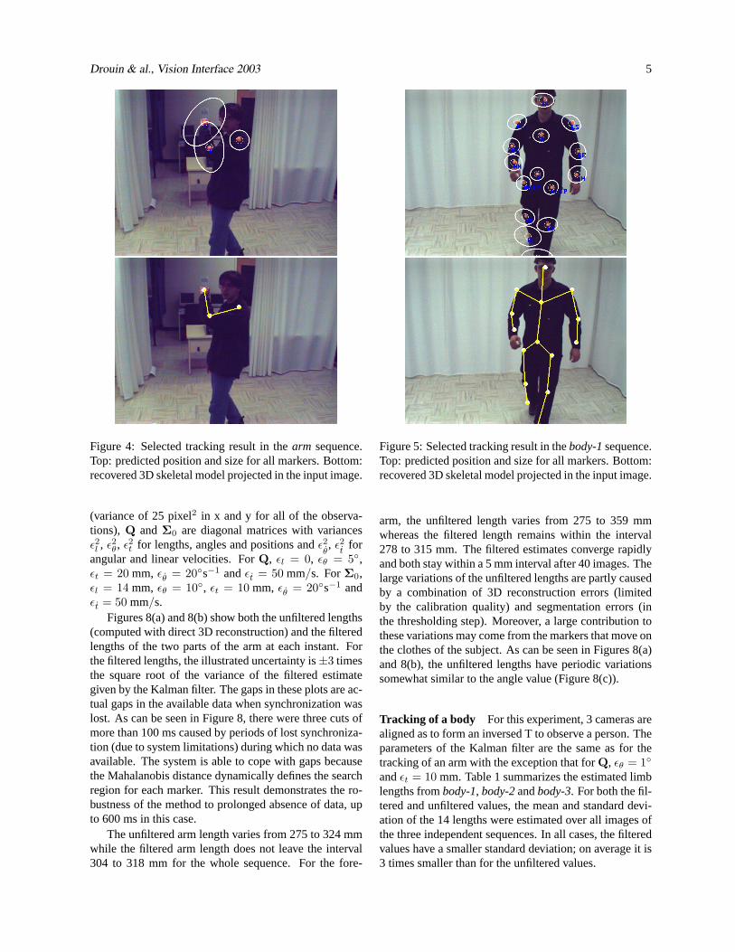
4 ResultsA set of calibrated and synchronized sequences are usedfor the experiments. Thearm sequence (Figure 4) wasacquired with a system of 4 cameras and contains 162images/camera. Three sequences of the whole body (Fig-ures 5 to 7) were acquired with a system of 3 camerasand are composed of 317, 311 and 170 images, respec-tively. In these results, the large ellipses are the searchregions for each marker defined by a Mahalanobis dis-tance of 9.21 to the predicted position. The circle at thecenter of each ellipse is the maximum predicted size foreach marker.

Tracking of an arm For this experiment, 4 cameras areplaced in an half-circle arrangement and observe the armof a person. Orange balls are placed on the shoulder, theelbow and the hand; they are segmented in the four im-ages to produce the observations of the system. The pa-rameters of the Kalman filter are as follows:R = 25I


Figure 4: Selected tracking result in thearm sequence.Top: predicted position and size for all markers. Bottom:recovered 3D skeletal model projected in the input image.

(variance of 25 pixel2 in x and y for all of the observa-tions), Q andΣ0 are diagonal matrices with variancesε2l , ε2θ, ε2t for lengths, angles and positions andε2

θ, ε2

tfor

angular and linear velocities. ForQ, εl = 0, εθ = 5◦,εt = 20 mm, εθ = 20◦s−1 andεt = 50 mm/s. ForΣ0,εl = 14 mm, εθ = 10◦, εt = 10 mm, εθ = 20◦s−1 andεt = 50 mm/s.

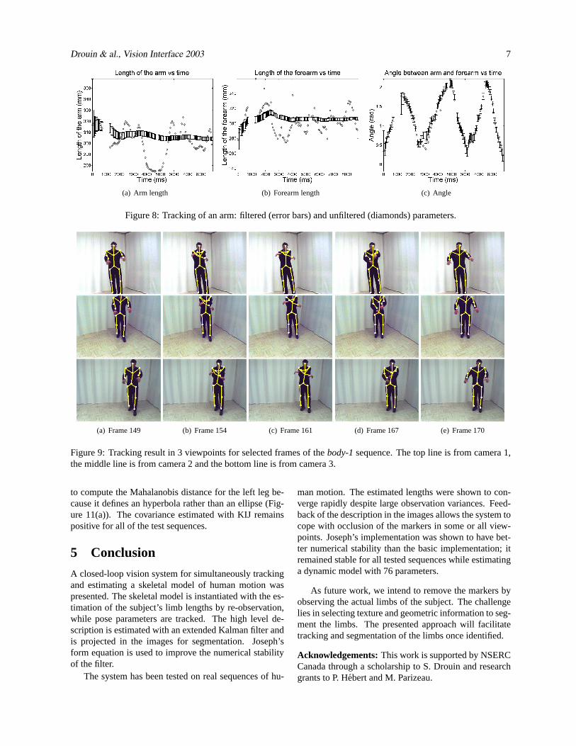
Figures 8(a) and 8(b) show both the unfiltered lengths(computed with direct 3D reconstruction) and the filteredlengths of the two parts of the arm at each instant. Forthe filtered lengths, the illustrated uncertainty is±3 timesthe square root of the variance of the filtered estimategiven by the Kalman filter. The gaps in these plots are ac-tual gaps in the available data when synchronization waslost. As can be seen in Figure 8, there were three cuts ofmore than 100 ms caused by periods of lost synchroniza-tion (due to system limitations) during which no data wasavailable. The system is able to cope with gaps becausethe Mahalanobis distance dynamically defines the searchregion for each marker. This result demonstrates the ro-bustness of the method to prolonged absence of data, upto 600 ms in this case.

The unfiltered arm length varies from 275 to 324 mmwhile the filtered arm length does not leave the interval304 to 318 mm for the whole sequence. For the fore-

Figure 5: Selected tracking result in thebody-1sequence.Top: predicted position and size for all markers. Bottom:recovered 3D skeletal model projected in the input image.

arm, the unfiltered length varies from 275 to 359 mmwhereas the filtered length remains within the interval278 to 315 mm. The filtered estimates converge rapidlyand both stay within a 5 mm interval after 40 images. Thelarge variations of the unfiltered lengths are partly causedby a combination of 3D reconstruction errors (limitedby the calibration quality) and segmentation errors (inthe thresholding step). Moreover, a large contribution tothese variations may come from the markers that move onthe clothes of the subject. As can be seen in Figures 8(a)and 8(b), the unfiltered lengths have periodic variationssomewhat similar to the angle value (Figure 8(c)).

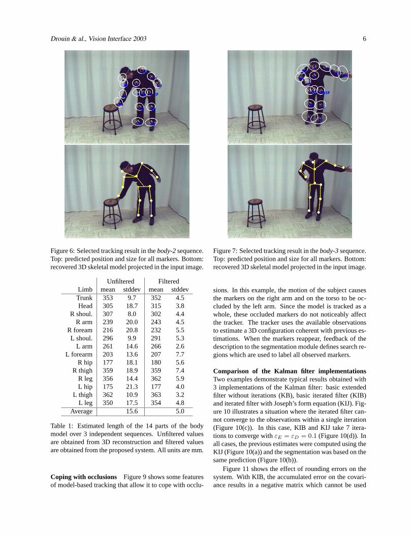
Tracking of a body For this experiment, 3 cameras arealigned as to form an inversed T to observe a person. Theparameters of the Kalman filter are the same as for thetracking of an arm with the exception that forQ, εθ = 1◦

andεt = 10 mm. Table 1 summarizes the estimated limblengths frombody-1, body-2andbody-3. For both the fil-tered and unfiltered values, the mean and standard devi-ation of the 14 lengths were estimated over all images ofthe three independent sequences. In all cases, the filteredvalues have a smaller standard deviation; on average it is3 times smaller than for the unfiltered values.



Unfiltered FilteredLimb mean stddev mean stddevTrunk 353 9.7 352 4.5Head 305 18.7 315 3.8

R shoul. 307 8.0 302 4.4R arm 239 20.0 243 4.5

R foream 216 20.8 232 5.5L shoul. 296 9.9 291 5.3

L arm 261 14.6 266 2.6L forearm 203 13.6 207 7.7

R hip 177 18.1 180 5.6R thigh 359 18.9 359 7.4

R leg 356 14.4 362 5.9L hip 175 21.3 177 4.0

L thigh 362 10.9 363 3.2L leg 350 17.5 354 4.8

Average 15.6 5.0

Table 1: Estimated length of the 14 parts of the bodymodel over 3 independent sequences. Unfiltered valuesare obtained from 3D reconstruction and filtered valuesare obtained from the proposed system. All units are mm.

Coping with occlusions Figure 9 shows some featuresof model-based tracking that allow it to cope with occlu-


sions. In this example, the motion of the subject causesthe markers on the right arm and on the torso to be oc-cluded by the left arm. Since the model is tracked as awhole, these occluded markers do not noticeably affectthe tracker. The tracker uses the available observationsto estimate a 3D configuration coherent with previous es-timations. When the markers reappear, feedback of thedescription to the segmentation module defines search re-gions which are used to label all observed markers.

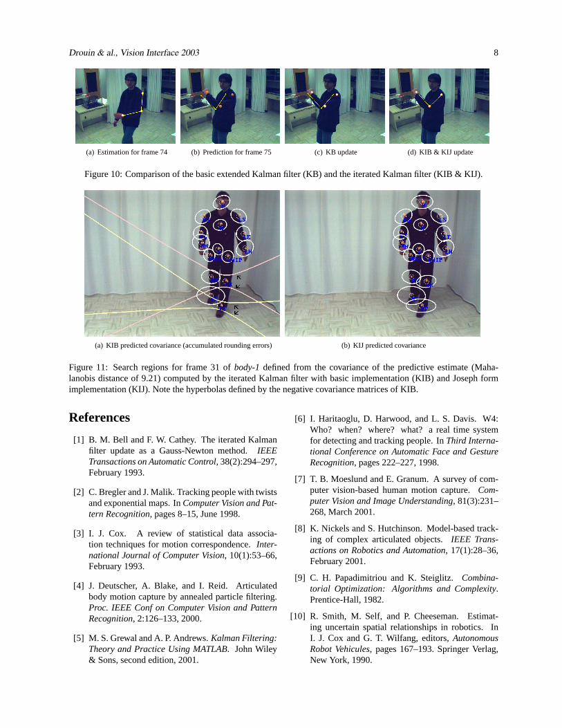
Comparison of the Kalman filter implementationsTwo examples demonstrate typical results obtained with3 implementations of the Kalman filter: basic extendedfilter without iterations (KB), basic iterated filter (KIB)and iterated filter with Joseph’s form equation (KIJ). Fig-ure 10 illustrates a situation where the iterated filter can-not converge to the observations within a single iteration(Figure 10(c)). In this case, KIB and KIJ take 7 itera-tions to converge withεE = εD = 0.1 (Figure 10(d)). Inall cases, the previous estimates were computed using theKIJ (Figure 10(a)) and the segmentation was based on thesame prediction (Figure 10(b)).

Figure 11 shows the effect of rounding errors on thesystem. With KIB, the accumulated error on the covari-ance results in a negative matrix which cannot be used


(a) Arm length (b) Forearm length (c) Angle

Figure 8: Tracking of an arm: filtered (error bars) and unfiltered (diamonds) parameters.

(a) Frame 149 (b) Frame 154 (c) Frame 161 (d) Frame 167 (e) Frame 170

Figure 9: Tracking result in 3 viewpoints for selected frames of thebody-1sequence. The top line is from camera 1,the middle line is from camera 2 and the bottom line is from camera 3.

to compute the Mahalanobis distance for the left leg be-cause it defines an hyperbola rather than an ellipse (Fig-ure 11(a)). The covariance estimated with KIJ remainspositive for all of the test sequences.

5 Conclusion

A closed-loop vision system for simultaneously trackingand estimating a skeletal model of human motion waspresented. The skeletal model is instantiated with the es-timation of the subject’s limb lengths by re-observation,while pose parameters are tracked. The high level de-scription is estimated with an extended Kalman filter andis projected in the images for segmentation. Joseph’sform equation is used to improve the numerical stabilityof the filter.

The system has been tested on real sequences of hu-

man motion. The estimated lengths were shown to con-verge rapidly despite large observation variances. Feed-back of the description in the images allows the system tocope with occlusion of the markers in some or all view-points. Joseph’s implementation was shown to have bet-ter numerical stability than the basic implementation; itremained stable for all tested sequences while estimatinga dynamic model with 76 parameters.

As future work, we intend to remove the markers byobserving the actual limbs of the subject. The challengelies in selecting texture and geometric information to seg-ment the limbs. The presented approach will facilitatetracking and segmentation of the limbs once identified.

Acknowledgements:This work is supported by NSERCCanada through a scholarship to S. Drouin and researchgrants to P. Hebert and M. Parizeau.


(a) Estimation for frame 74 (b) Prediction for frame 75 (c) KB update (d) KIB & KIJ update

Figure 10: Comparison of the basic extended Kalman filter (KB) and the iterated Kalman filter (KIB & KIJ).

(a) KIB predicted covariance (accumulated rounding errors) (b) KIJ predicted covariance

Figure 11: Search regions for frame 31 ofbody-1defined from the covariance of the predictive estimate (Maha-lanobis distance of 9.21) computed by the iterated Kalman filter with basic implementation (KIB) and Joseph formimplementation (KIJ). Note the hyperbolas defined by the negative covariance matrices of KIB.

References

[1] B. M. Bell and F. W. Cathey. The iterated Kalmanfilter update as a Gauss-Newton method.IEEETransactions on Automatic Control, 38(2):294–297,February 1993.

[2] C. Bregler and J. Malik. Tracking people with twistsand exponential maps. InComputer Vision and Pat-tern Recognition, pages 8–15, June 1998.

[3] I. J. Cox. A review of statistical data associa-tion techniques for motion correspondence.Inter-national Journal of Computer Vision, 10(1):53–66,February 1993.

[4] J. Deutscher, A. Blake, and I. Reid. Articulatedbody motion capture by annealed particle filtering.Proc. IEEE Conf on Computer Vision and PatternRecognition, 2:126–133, 2000.

[5] M. S. Grewal and A. P. Andrews.Kalman Filtering:Theory and Practice Using MATLAB. John Wiley& Sons, second edition, 2001.

[6] I. Haritaoglu, D. Harwood, and L. S. Davis. W4:Who? when? where? what? a real time systemfor detecting and tracking people. InThird Interna-tional Conference on Automatic Face and GestureRecognition, pages 222–227, 1998.

[7] T. B. Moeslund and E. Granum. A survey of com-puter vision-based human motion capture.Com-puter Vision and Image Understanding, 81(3):231–268, March 2001.

[8] K. Nickels and S. Hutchinson. Model-based track-ing of complex articulated objects.IEEE Trans-actions on Robotics and Automation, 17(1):28–36,February 2001.

[9] C. H. Papadimitriou and K. Steiglitz.Combina-torial Optimization: Algorithms and Complexity.Prentice-Hall, 1982.

[10] R. Smith, M. Self, and P. Cheeseman. Estimat-ing uncertain spatial relationships in robotics. InI. J. Cox and G. T. Wilfang, editors,AutonomousRobot Vehicules, pages 167–193. Springer Verlag,New York, 1990.

Documents

Simultaneous Tracking and Estimation of a Skeletal Model