SIMXManual - Harvard Universityhea- · SIMXManual for ASTRO-H members ... (Center for Astrophysics) ... simxhome page at CfA

SIMX Manualfor ASTRO-H members

updated for version 2.1.0

Hiroya Yamaguchi and Kosuke Sato

Directed by Randall K. Smith

June 20, 2014

Members

SIMX Working Group members

Randall K. Smith (Harvard-Smithsonian Center for Astrophysics)

Laura Brenneman (Harvard-Smithsonian Center for Astrophysics)

Kosuke Sato (Tokyo University of Science)

Emeritus: Hiroya Yamaguchi (Center for Astrophysics)

Contact us if you have any question about [email protected]

simx home page at CfAhttp://hea-www.harvard.edu/simx/index.html(The latest version can be found at this URL.)

Wiki page for the ASTRO-H membershttp://www.astro.isas.jaxa.jp/next/astroh-simx/wiki/index.php?FrontPage

Chapter 1

What is “SIMX”?

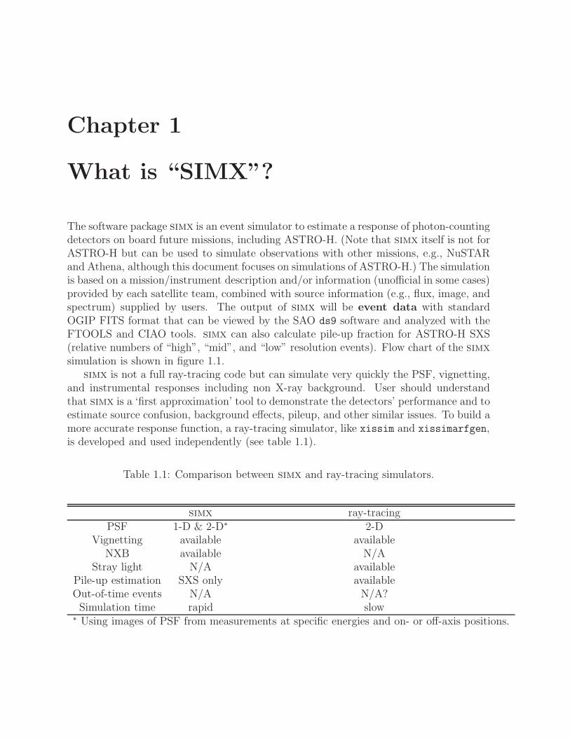
The software package simx is an event simulator to estimate a response of photon-countingdetectors on board future missions, including ASTRO-H. (Note that simx itself is not forASTRO-H but can be used to simulate observations with other missions, e.g., NuSTARand Athena, although this document focuses on simulations of ASTRO-H.) The simulationis based on a mission/instrument description and/or information (unofficial in some cases)provided by each satellite team, combined with source information (e.g., flux, image, andspectrum) supplied by users. The output of simx will be event data with standardOGIP FITS format that can be viewed by the SAO ds9 software and analyzed with theFTOOLS and CIAO tools. simx can also calculate pile-up fraction for ASTRO-H SXS(relative numbers of “high”, “mid”, and “low” resolution events). Flow chart of the simxsimulation is shown in figure 1.1.

simx is not a full ray-tracing code but can simulate very quickly the PSF, vignetting,and instrumental responses including non X-ray background. User should understandthat simx is a ‘first approximation’ tool to demonstrate the detectors’ performance and toestimate source confusion, background effects, pileup, and other similar issues. To build amore accurate response function, a ray-tracing simulator, like xissim and xissimarfgen,is developed and used independently (see table 1.1).

Table 1.1: Comparison between simx and ray-tracing simulators.

simx ray-tracingPSF 1-D & 2-D∗ 2-D

Vignetting available availableNXB available N/A

Stray light N/A availablePile-up estimation SXS only availableOut-of-time events N/A N/A?Simulation time rapid slow

∗ Using images of PSF from measurements at specific energies and on- or off-axis positions.

2 CHAPTER 1. WHAT IS “SIMX”?

Image Spectrum

Source information

FITS data text table (qdp) data

SIMX

Instrument information

- Effective area

- PSF- Vignetting

- Detector response

Event data

DS9 XSELECT

+ Pile-up info (for SXS)

Simulated data

XSPEC

RMF + ARFImage Spectrum

Figure 1.1: Flow chart of simulation using simx. — Note: Source image and spectrumare optional. A point-like source or a monochromatic-energy spectrum can be simulatedwithout them. For spectral analysis, an ARF file should be created separately (usingsomething like xissimarfgen), although the simx package contains some representativeARFs (e.g., one for a point source with r < 1.′8).

Chapter 2

Installation and Setup

2.1 Installation

simx is distributed as a source code, and requires C compiler to install. It has been testedon Linux and Mac OS X. After downloading the simx tarball from the URL,http://hea-www.harvard.edu/simx/download.html

execute the following commands to compile and install the code:

unix% tar zxf simx-X.Y.Z.tar.gz

unix% tar cd simx-X.Y.Z

unix% ./configure

unix% make

unix% make install

If the code is compiled correctly, you should now have a bin directory with a copy ofsimx. We have tested this on Mac’s running 10.6-10.9 (Snow Leopard-Mavericks) and aLinux machine running Scientific Linux 5, Kernel 2.6.18-371.6.1.

If you would like to test your version, you can then run the following commands (warn-ing: test comparisons require that you have FTOOLS installed and ready to run):

unix% cd test

unix% make test

Please report any odd behavior on the part of the code to:[email protected]

When reporting problems, please don’t hesitate to look at the code and suggest fixes.

Notes from the Field

1. The ’make install’ step is required. Otherwise, simx will bomb out immediatelycomplaining that it cannot find the simx par file.

2. In some cases, the make command will fail with a message along the lines of “ld:in ../src/libsimx.a, archive has no table of contents”. In this case, youmay be able to fix the problem by typing “cd src ; ranlib libsimx.a ; cd ..”.

3. If run on a 32-bit computer, make test may fail on the Cas A simulation withthe Astro-H SXI, reporting differences in the number of events. However, the dif-ferent numbers are quite close to the canonical values, and the difference is likely

4 CHAPTER 2. INSTALLATION AND SETUP

due to differences in how the random number function works on 32-bit and 64-bitcomputers. This can be ignored, as it should not be a problem with running simx.

2.2 Setup

2.2.1 Setting up to run simx

The mission and/or instrument description is provided by data in the file xselect.mdb,in the simx/inputs directory. simx must be able to find this file as a default, which itdoes via the simx system variable. This is set by the simx-setup.csh or –.sh script,found in simx/bin. Thus, before running simx, you must first run the setup script via:

unix% source /path/to/simx/bin/simx-setup.csh (for CSH version)unix% ./path/to/simx/bin/simx-setup.csh (for BASH version)

2.2.2 Running simx

simx uses the ever-popular IRAF interface that should be familiar to FTOOLS and CIAOusers. It expects to find its parameter file in a directory pointed to by the PFILES systemvariable. If you are an FTOOLS user, you probably have a directory ‘pfiles’ in your homedirectory, e.g., /home/user/pfiles. Running simx-setup.[csh/sh] as shown above willset up the PFILES environment properly so that this is done automatically. However, itcan be done directly as well using:

unix% cp /path/to/simx/pfiles/simx.par /home/user/pfiles/simx.par

Alternatively, you can simply set the PFILES environment variable to point to thepfiles directory in simx:

unix% setenv PFILES /path/to/simx/pfiles (for CSH version)

unix% set PFILES /path/to/simx/pfiles

unix% export PFILES (for BASH version)

Note that the syspfiles directory contains a ‘pristine’ version of the same file in casethe one in pfiles is corrupted somehow.

To run simx, simply set the simulation parameters in simx.par to the desired val-ues by editing the file directly in an editor (this method is somewhat risky) or installingFTOOLS and using pset, e.g.:

unix% pset simx OutputFileName = MySimRun

unix% pset simx Exposure = 10000

(see also chapter 3) and then run simx:

unix% /path/to/simx/bin/simx

2.2. SETUP 5

The code will generate an output event file in the current directory which can beviewed with ds9 or used with the CIAO tools dmextract or the FTOOLS xselect. Thespecially-modified version of xselect.mdb is needed to use these files with xselect. Touse this file with xselect instead of the default xselect.mdb that comes with FTOOLS,set the following environment variable:

unix% setenv XSELECT MDB /path/to/simx/inputs/xselect.mdb (for CSH version)

unix% set XSELECT MDB /path/to/simx/inputs/xselect.mdb

unix% export XSELECT MDB (for BASH version)

After that, xselect will automatically pick up the correct mission when the simx outputfiles are read and will use the proper binning and column names for the extraction.

Chapter 3

Input Parameters & Files

3.1 Standard parameter options

As explained in the previous chapter, the input parameter list for simulation can bemodified by using the pset command, but you can also give the parameters listed belowinteractively after running the simx program.

• OutputFileName: ‘Output Event file stem[ ]’; The output event file namestem. Final event file name will be this step with “ evt.fits” appended.

• PointingRA: ‘Pointing right ascension (decimal degrees)[ ]’; Right As-cension (in decimal degrees) of the pointing direction of the satellite.

• PointingDec: ‘Pointing declination (decimal degrees)[ ]’; Declination (indecimal degrees) of the pointing direction of the satellite.

• Exposure: ‘Exposure time (seconds)[ ]’; Exposure time (in seconds).

• SourceFlux: ‘Source Flux in erg/cm^2/s[ ]’; Total source flux (in erg cm−2

s−1). The energy range of the flux must match the range of the model spectrum.

• SourceImageType: ‘Source Image Type (Point|Flat|Image)[ ]’; One of Point,Flat, or Image; If Point is chosen, the point source position must be provided as the“SourcePointRA” and “SourcePointDec” parameters. If Image is chosen, a FITSimage file must be provided in “SourceImageFile”. If Flat is chosen, neither posi-tion parameter nor input image is needed but flat-surface-brightness sky is assumed.The input flux is assumed to be that of the entire FoV of the individual instrument:(Flux) = (Surface brightness) × (FoV size). The angular size of the FoV of eachinstrument aboard ASTRO-H is listed in Table 3.1.

• SourcePointRA: ‘Source right ascension (decimal degrees)[ ]’; Right As-cension (in decimal degrees) of the point source; only used when “SourceImageType= Point”. If you aim to simulate an on-axis observation, this and the ‘SourcePoint-Dec” values should match “PointingRA” and “PointingDec”.

• SourcePointDec: ‘Source declination (decimal degrees)[ ]’; Declination (indecimal degrees) of the point source; only used when “SourceImageType = Point”.

• SourceImageFile: ‘Source Image File[ ]’; FITS-format file containing the im-age to simulate; only used when “SourceImageType = Image”.

3.2. NON-STANDARD OPTIONS 7

• SourceSpectrumType: ‘Source Spectrum Type (XSPEC File|Sherpa File|Mono)[ ]’;One of XSPEC File, Sherpa File, or Mono. If set to Mono, the source is assumedto be monoenergetic with the energy set in the “MonoEnergy” parameter. IfXSPEC File, it is assumed the spectrum is output from XSPEC using the com-mandsXSPEC> ...define model spectrum...

XSPEC> plot model

XSPEC> iplot

PLT> wdata model.dat

PLT> quit

In this case, the file will have at least 3 columns, Energy (in keV), delta-Energy,and flux (in photons/cm2/s/keV); the first three rows are ignored as they normallycontain text.If Sherpa File is the parameter, it is assumed the spectrum file comes from a Sherpamodel created (in CIAO 3) via:sherpa> ...define model spectrum...

sherpa> write source source.dat

In this case, the file will have 2 columns, Energy (in keV), and Flux (in photons/cm2/s/keV).If you generate the spectrum file some other way than XSPEC or Sherpa, simplyoutput the spectrum in this format (two columns, energy and flux) and simx shouldbe able to read it.

• SourceSpectrumFile: ‘Source Spectrum File[ ]’; The name of the source spec-trum file, if “SourceSpectrumType = XSPEC File or Sherpa File” (see next).

• MonoEnergy: ‘Energy (in keV) if monoenergetic[ ]’; The energy (in keV)of the mono-energetic spectrum if “SourceSpectrumType = Mono”.

• RandomSeed: ‘Initial Random Seed; use -1 to generate internally[0]’;The initial random seed. If you set this to -1, the code will use the current time toseed the random number generator, while any other value will always generate thesame sequence of random numbers.

• MissionName: ‘Mission Name[ ]’; Available missions are summarized in Sec-tion 3.3.

• InstrumentName: ‘Instrument Name[ ]’; Allowable settings for this dependupon the “MissionName” setting. See Section 3.3.

• FilterName: ‘Filter Name[ ]’; Allowable settings for this depend upon the “In-strumentName” setting. See Section 3.3.

• ScaleBkgnd: ‘Linear scaling factor for testing background sensitivity

(0.0:10.0) [1.0]’ Linear scaling factor for the background. By default set to 1.0,but can be varied to test the impact of higher or lower background level.

3.2 Non-standard options

You can also change the parameters given below by using the pset command, althoughthese are not able to be changed interactively when simx is running. The default of

8 CHAPTER 3. INPUT PARAMETERS & FILES

the first three parameters is “$XSELECT MDB”. The xselect.mdb file is found in thesimx/inputs directory.

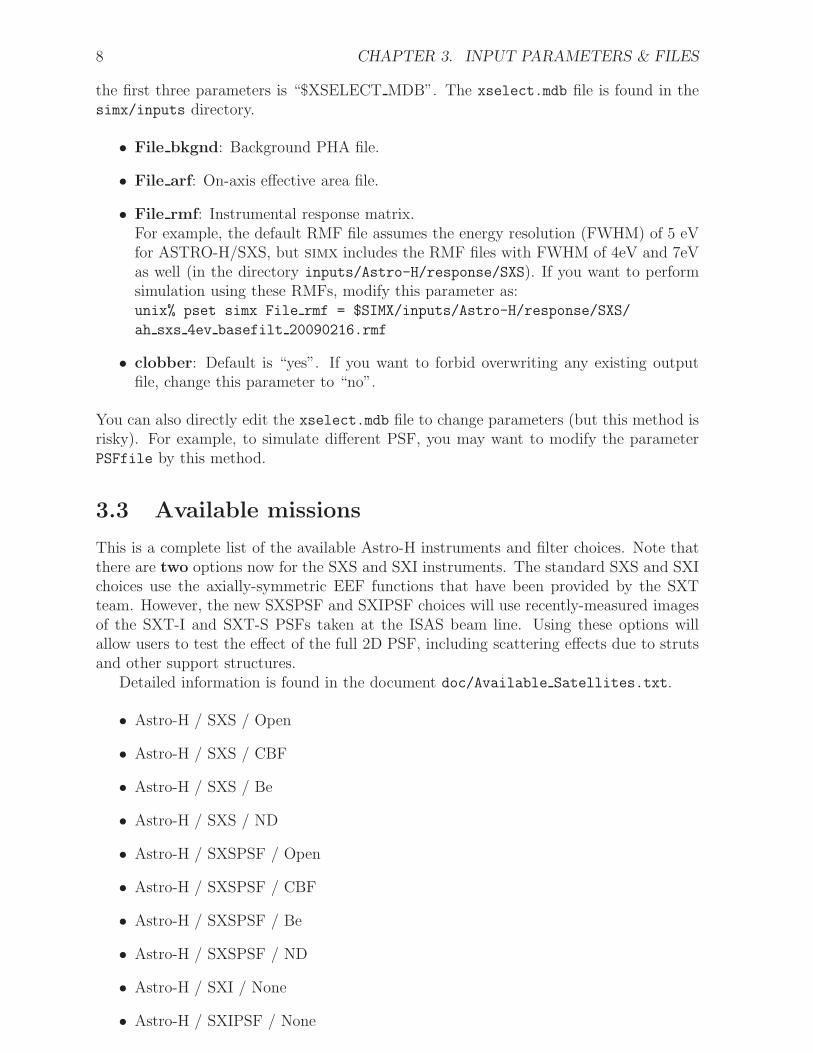
• File bkgnd: Background PHA file.

• File arf: On-axis effective area file.

• File rmf: Instrumental response matrix.For example, the default RMF file assumes the energy resolution (FWHM) of 5 eVfor ASTRO-H/SXS, but simx includes the RMF files with FWHM of 4eV and 7eVas well (in the directory inputs/Astro-H/response/SXS). If you want to performsimulation using these RMFs, modify this parameter as:unix% pset simx File rmf = $SIMX/inputs/Astro-H/response/SXS/

ah sxs 4ev basefilt 20090216.rmf

• clobber: Default is “yes”. If you want to forbid overwriting any existing outputfile, change this parameter to “no”.

You can also directly edit the xselect.mdb file to change parameters (but this method isrisky). For example, to simulate different PSF, you may want to modify the parameterPSFfile by this method.

3.3 Available missions

This is a complete list of the available Astro-H instruments and filter choices. Note thatthere are two options now for the SXS and SXI instruments. The standard SXS and SXIchoices use the axially-symmetric EEF functions that have been provided by the SXTteam. However, the new SXSPSF and SXIPSF choices will use recently-measured imagesof the SXT-I and SXT-S PSFs taken at the ISAS beam line. Using these options willallow users to test the effect of the full 2D PSF, including scattering effects due to strutsand other support structures.

Detailed information is found in the document doc/Available Satellites.txt.

• Astro-H / SXS / Open

• Astro-H / SXS / CBF

• Astro-H / SXS / Be

• Astro-H / SXS / ND

• Astro-H / SXSPSF / Open

• Astro-H / SXSPSF / CBF

• Astro-H / SXSPSF / Be

• Astro-H / SXSPSF / ND

• Astro-H / SXI / None

• Astro-H / SXIPSF / None

3.4. DESIGN PARAMETERS OF ASTRO-H 9

• Astro-H / HXI / None

• Astro-H / HXI-toponly / None

• Astro-H / SGD / None

3.4 Design parameters of ASTRO-H

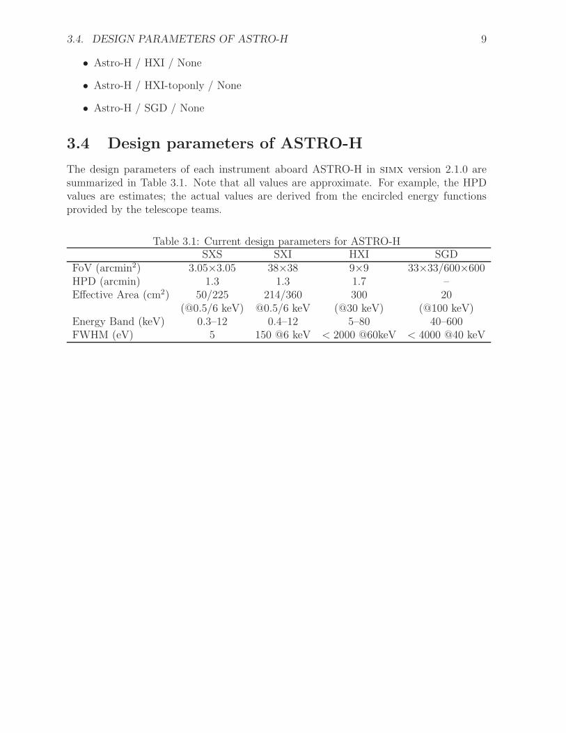
The design parameters of each instrument aboard ASTRO-H in simx version 2.1.0 aresummarized in Table 3.1. Note that all values are approximate. For example, the HPDvalues are estimates; the actual values are derived from the encircled energy functionsprovided by the telescope teams.

Table 3.1: Current design parameters for ASTRO-HSXS SXI HXI SGD

FoV (arcmin2) 3.05×3.05 38×38 9×9 33×33/600×600HPD (arcmin) 1.3 1.3 1.7 –Effective Area (cm2) 50/225 214/360 300 20

(@0.5/6 keV) @0.5/6 keV (@30 keV) (@100 keV)Energy Band (keV) 0.3–12 0.4–12 5–80 40–600FWHM (eV) 5 150 @6 keV < 2000 @60keV < 4000 @40 keV

Chapter 4

Tutorial 1: Simple Simulation

4.1 SXS for a thermal X-ray source

In this section, we learn how to run simx assuming a virtual point-like source with a simpleoptically-thin thermal plasma spectrum. The latest version of simx is v2.1.0. Hereafter,users are assumed to use this version.

Preparing input model spectra

simx can simulate not only monoenergetic events but also an arbitrary model spectrum.In the latter case, we need to prepare a spectral data prior to running simx. The spectrumis assumed to be output from either XSPEC or Sherpa. The XSPEC-type spectrum data havethree columns of Energy (in keV), delta-energy (in keV), and flux (in photon/cm2/s/keV).The first three rows normally contain text (e.g., “READ SERR 1”) which will be ignoredin the simx simulation. On the other hand, the Sherpa-type spectrum has only twocolumns, Energy (in keV) and flux (in photon/cm2/s/keV).

Important note : To derive an appropriate simulation result, an input spectrum shouldhave sufficiently small bin size. Since the energy bin of the SXS RMF is given for each1 eV, users are recommended to create a model spectrum with the energy bin of 1 eV or lessfor SXS (and SXI) simulation. Otherwise, an incorrect result will potentially be obtained.

Using XSPEC, we here create a model spectrum of a thermal plasma in collisional ion-ization equilibrium (APEC model; Smith et al. 2001) with an electron temperature kT

e

of 2.0 keV, absorbed by a hydrogen column density NH of 1× 1021 cm−2.

unix% xspec

XSPEC12>dummyrsp 0.1 10 9900 linear < − important!XSPEC12>model wabs * apec

1:wabs:nH>0.1

2:apec:kT>2

3:apec:Abundanc>1

4:apec:redshift>0

5:apec:norm>1

Important note : Here you don’t need to care about normalization. simx uses only theshape of the spectrum from the input data, while the normalization is given by the input

4.1. SXS FOR A THERMAL X-RAY SOURCE 11

0.1 1 10

10−

30.

010.

11

10

Pho

tons

cm−

2 s−

1 ke

V−

1

Energy (keV)10.5 2

0.1

110

Pho

tons

cm−

2 s−

1 ke

V−

1

Energy (keV)

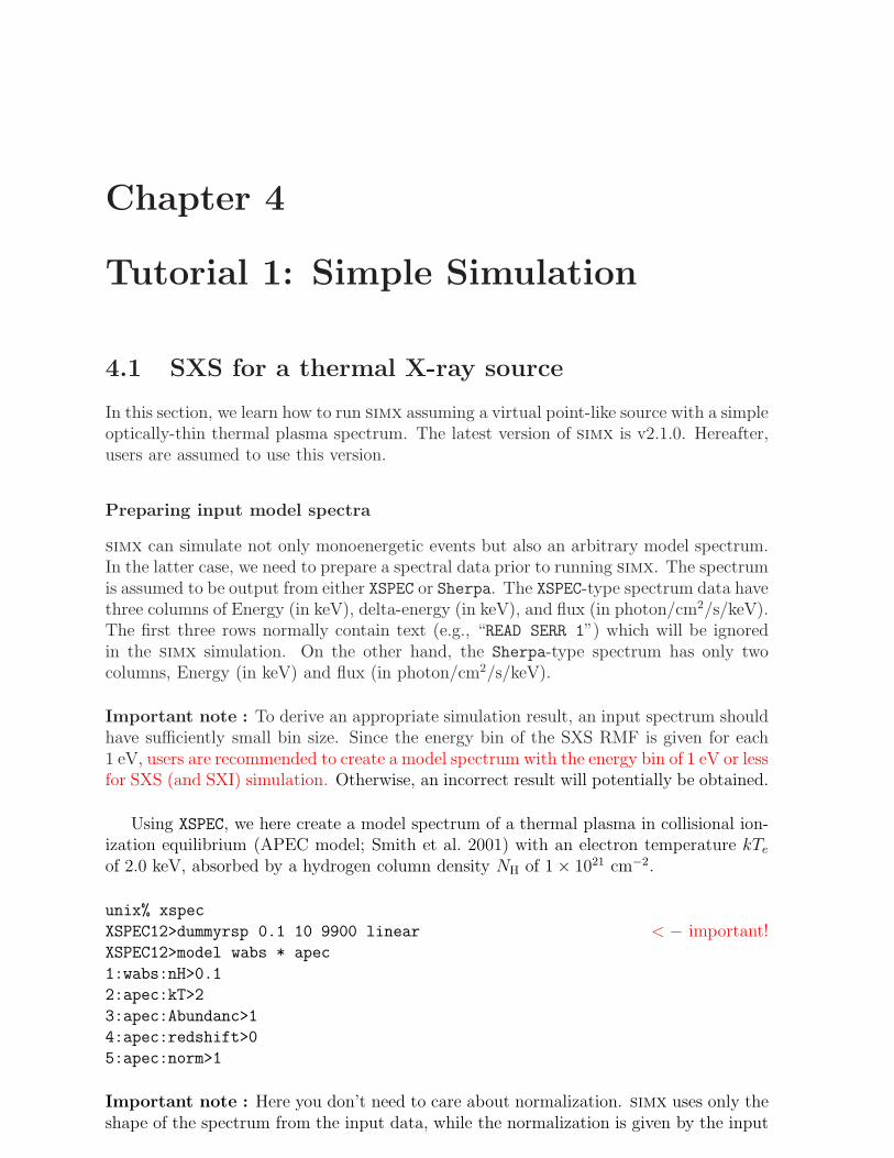
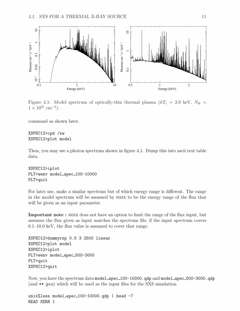
Figure 4.1: Model spectrum of optically-thin thermal plasma (kTe= 2.0 keV, NH =

1× 1021 cm−2).

command as shown later.

XSPEC12>cpd /xw

XSPEC12>plot model

Then, you may see a photon spectrum shown in figure 4.1. Dump this into ascii text tabledata.

XSPEC12>iplot

PLT>wenv model apec 100-10000

PLT>quit

For later use, make a similar spectrum but of which energy range is different. The rangein the model spectrum will be assumed by simx to be the energy range of the flux thatwill be given as an input parameter.

Important note : simx does not have an option to limit the range of the flux input, butassumes the flux given as input matches the spectrum file; if the input spectrum covers0.1–10.0 keV, the flux value is assumed to cover that range.

XSPEC12>dummyrsp 0.5 3 2500 linear

XSPEC12>plot model

XSPEC12>iplot

PLT>wenv model apec 500-3000

PLT>quit

XSPEC12>quit

Now, you have the spectrum data model apec 100-10000.qdp and model apec 500-3000.qdp

(and **.pco) which will be used as the input files for the SXS simulation.

unix%less model apec 100-10000.qdp | head -7

READ SERR 1

12 CHAPTER 4. TUTORIAL 1: SIMPLE SIMULATION

@model apec 100-10000.pco

!

0.1005 5.00000024E-4 0

0.1015 5.00000024E-4 0

0.1025 5.00000024E-4 0

0.1035 5.00000024E-4 0

unix%less model apec 100-10000.qdp | tail -4

9.9965 5.00000024E-4 2.02651878E-4

9.9975004 5.00000024E-4 2.02720272E-4

9.9984999 5.00000024E-4 2.0240208E-4

9.9995003 5.00000024E-4 2.02512281E-4

unix%less model apec 500-3000.qdp | head -7

READ SERR 1

@model apec 500-3000.pco

!

0.50050002 5.00000024E-4 1.4454185

0.50150001 5.00000024E-4 0.43789926

0.5025 5.00000024E-4 0.40159792

0.50349998 5.00000024E-4 0.39090225

unix%less model apec 500-3000.qdp | tail -4

2.9965 5.00000024E-4 2.61854846E-2

2.9974999 5.00000024E-4 2.61666924E-2

2.9985001 5.00000024E-4 2.61504054E-2

2.9995 5.00000024E-4 2.61206795E-2

Running simx

You are now ready to run simx. However, you can set the input parameter before simx isexecuted. (This process can be skipped, if you prefer to input the parameters interactivelyafter running simx.)

Set the stem of the output event file name.unix%pset simx OutputFileName=AH SXS point apec 100-10000

(The file name will be this with ” evt.fits” appended.)

Set the pointing position.unix%pset simx PointingRA = 0.0

unix%pset simx PointingDec = 0.0

Set the exposure (in sec).unix%pset simx Exposure=50000

Set the flux (in erg/cm−2/s).unix%pset simx SourceFlux=1e-10

Set the input image or pointing position. (Here we simulate a point-like source. There


are other options, Flat and Image, which will be explained in the next chapter.)unix%pset simx SourceImageType=Point

unix%pset simx SourcePointRA=0.0

unix%pset simx SourcePointDec=0.0

unix%pset simx SourceImageFile=None

Set the input spectrum.unix%pset simx SourceSpectrumType=XSPEC File

unix%pset simx SourceSpectrumFile=model apec 100-10000.qdp

Set the mission/instrument/filter names.unix%pset simx MissionName=Astro-H

unix%pset simx InstrumentName=SXS

unix%pset simx FilterName=Open

Set the linear scaling factor of the background level. The available range is from 0.0 to10.0. (This option is useful to investigate impact of change in the background level.)Here we simply ignore the background. unix%pset simx ScaleBkgnd=0.0

Finally, run simx to create an event file AH SXS point apec 100-10000 evt.fits. Do notforget setup simx:


unix%simx

**************************

*** simx version 2.1.0 ***

**************************

Output Event file stem[AH SXS point apec 100-10000]

Pointing right ascension (decimal degrees)[0.0]

Pointing declination (decimal degrees)[0.0]

Exposure time (seconds)[50000]

Use Simput File for source definition?[no]

Source Flux in erg/cm2/s[1e-10]

Source Image Type (Point|Flat|Image) [Point]

Source right ascension (decimal degrees)[0.0]

Source declination (decimal degrees)[0.0]

Source Image File[None]

Source Spectrum Type (XSPEC File|Sherpa File|Mono) [XSPEC File]

Source Spectrum File[model apec 100-10000.qdp]

Energy (in keV) if monoenergetic[2]

Initial Random Seed; use -1 to generate internally[0]

Mission Name[Astro-H]

Instrument Name[SXS]

Filter Name[Open]

Linear scaling factor for testing background sensitivity (0.1:10.0) [0.0]

...

...


...

generate events: Adding background events: 0

generate events: Actual number of events : 426148

...

...

generate events: Vignetted or otherwise lost events: 128497

generate events: Best-resolution events : 380102 ( 89.19%)

generate events: Mid-resolution events : 34412 ( 8.08%)

generate events: Low-resolution events : 11634 ( 2.73%)

The numbers of the detected and lost (to outside of the detector) events are displayed onyour terminal. For SXS simulation, the best-, mid-, and low-resolution event numbers arealso calculated.

Next, make another event file using the model spectrum with the energy range of 0.5–3.0 keV.

unix%pset simx OutputFileName=AH SXS point apec 500-3000

unix%pset simx SourceSpectrumFile=model apec 500-3000.qdp

unix%pset simx SourceFlux=1e-10

unix%simx

...

Keep in mind that the flux value assumed here is the same as that used in the previoussimulation.

Analyzing the output data

The output event data can be analyzed with the FTOOL XSELECT (or the other softwarepackages such as CIAO). Do not forget to modify the environment variable XSELECT MDB:

unix%setenv XSELECT MDB /path/to/simx/inputs/xselect.mdb (csh)unix%export XSELECT MDB=/path/to/simx/inputs/xselect.mdb (bash)

Otherwise, you will fail to read the event file with XSELECT and encounter with thefollowing error message:

Unidentified mission? :

Failed to identify instrument in MDB

Run XSELECT and read the SXS event file.

unix%xselect

...

...

xsel:*** > read event AH SXS point apec 100-10000 evt.fits

> Enter the Event file dir >[./]

Got new mission: ASTRO-H

> Reset the mission ? >[yes]

...


0 66 197 463 987 2046 4140 8309 16723 33366 66505

1 100.5 2 5

0.1

110

norm

aliz

ed c

ount

s s

−1

keV

−1

Energy (keV)

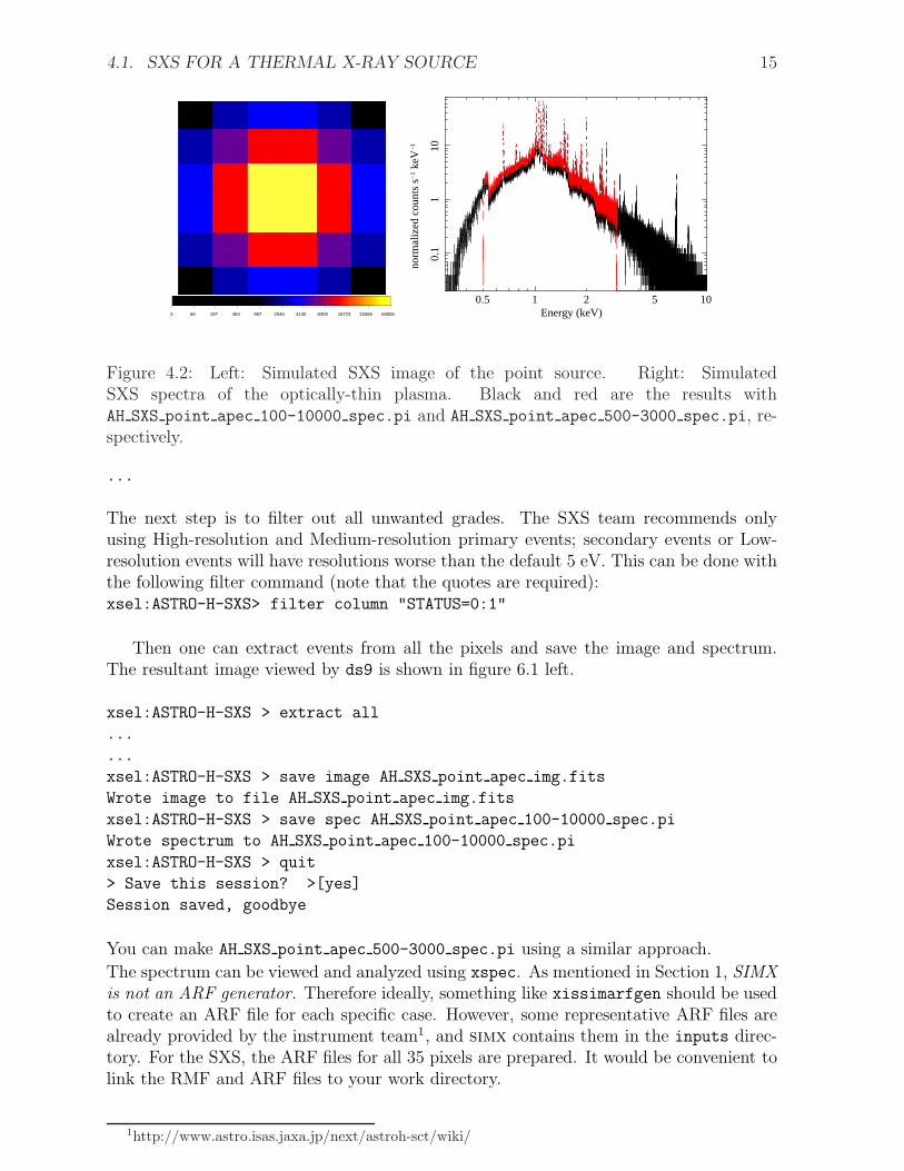
Figure 4.2: Left: Simulated SXS image of the point source. Right: SimulatedSXS spectra of the optically-thin plasma. Black and red are the results withAH SXS point apec 100-10000 spec.pi and AH SXS point apec 500-3000 spec.pi, re-spectively.

...

The next step is to filter out all unwanted grades. The SXS team recommends onlyusing High-resolution and Medium-resolution primary events; secondary events or Low-resolution events will have resolutions worse than the default 5 eV. This can be done withthe following filter command (note that the quotes are required):xsel:ASTRO-H-SXS> filter column "STATUS=0:1"

Then one can extract events from all the pixels and save the image and spectrum.The resultant image viewed by ds9 is shown in figure 6.1 left.

xsel:ASTRO-H-SXS > extract all

...

...

xsel:ASTRO-H-SXS > save image AH SXS point apec img.fits

Wrote image to file AH SXS point apec img.fits

xsel:ASTRO-H-SXS > save spec AH SXS point apec 100-10000 spec.pi

Wrote spectrum to AH SXS point apec 100-10000 spec.pi

xsel:ASTRO-H-SXS > quit

> Save this session? >[yes]

Session saved, goodbye

You can make AH SXS point apec 500-3000 spec.pi using a similar approach.

The spectrum can be viewed and analyzed using xspec. As mentioned in Section 1, SIMXis not an ARF generator. Therefore ideally, something like xissimarfgen should be usedto create an ARF file for each specific case. However, some representative ARF files arealready provided by the instrument team1, and simx contains them in the inputs direc-tory. For the SXS, the ARF files for all 35 pixels are prepared. It would be convenient tolink the RMF and ARF files to your work directory.

1http://www.astro.isas.jaxa.jp/next/astroh-sct/wiki/


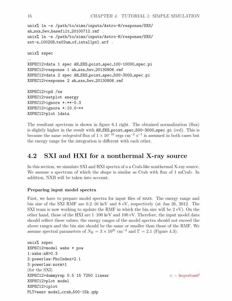
unix% ln -s /path/to/simx/inputs/Astro-H/response/SXS/

ah sxs 5ev basefilt 20100712.rmf .


sxt-s 100208 ts02um of intallpxl.arf .

unix% xspec

...XSPEC12>data 1 spec AH SXS point apec 100-10000 spec.pi

XSPEC12>response 1 ah sxs 5ev 20130806.rmf

XSPEC12>data 2 spec AH SXS point apec 500-3000 spec.pi

XSPEC12>response 2 ah sxs 5ev 20130806.rmf

XSPEC12>cpd /xw

XSPEC12>setplot energy

XSPEC12>ignore *:**-0.3

XSPEC12>ignore *:10.0-**

XSPEC12>plot ldata

The resultant spectrum is shown in figure 6.1 right. The obtained normalization (flux)is slightly higher in the result with AH SXS point apec 500-3000 spec.pi (red). This isbecause the same integrated flux of 1× 10−10 ergs cm−2 s−1 is assumed in both cases butthe energy range for the integration is different with each other.

4.2 SXI and HXI for a nonthermal X-ray source

In this section, we simulate SXI and HXI spectra of a a Crab-like nonthermal X-ray source.We assume a spectrum of which the shape is similar as Crab with flux of 1 mCrab. Inaddition, NXB will be taken into account.

Preparing input model spectra

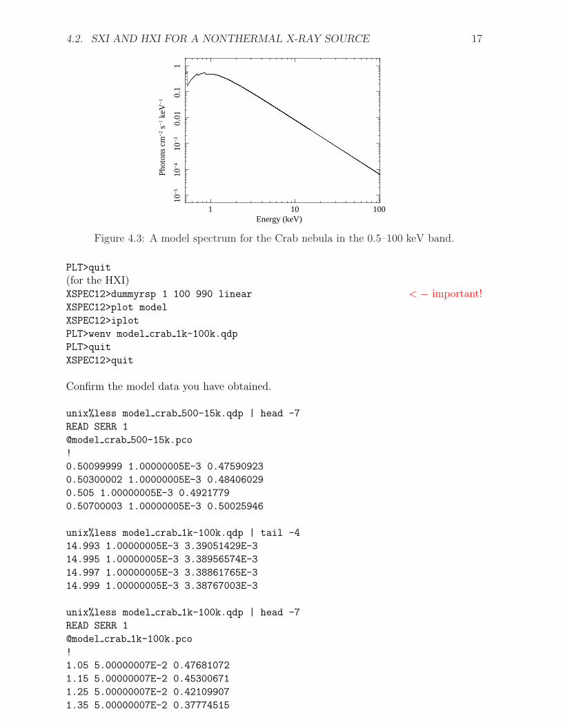
First, we have to prepare model spectra for input files of simx. The energy range andbin size of the SXI RMF are 0.2–16 keV and 8 eV, respectively (at Jan 26, 2012. TheSXI team is now working to update the RMF in which the bin size will be 2 eV). On theother hand, those of the HXI are 1–100 keV and 100 eV. Therefore, the input model datashould reflect these values; the energy ranges of the model spectra should not exceed theabove ranges and the bin size should be the same or smaller than those of the RMF. Weassume spectral parameters of NH = 3× 1021 cm−2 and Γ = 2.1 (Figure 4.3).

unix% xspec

XSPEC12>model wabs * pow

1:wabs:nH>0.3

2:powerlaw:PhoIndex>2.1

3:powerlaw:norm>1

(for the SXI)XSPEC12>dummyrsp 0.5 15 7250 linear < − important!XSPEC12>plot model

XSPEC12>iplot

PLT>wenv model crab 500-15k.qdp

4.2. SXI AND HXI FOR A NONTHERMAL X-RAY SOURCE 17

1 10 100

10−

510

−4

10−

30.

010.

11

Pho

tons

cm−

2 s−

1 ke

V−

1

Energy (keV)

Figure 4.3: A model spectrum for the Crab nebula in the 0.5–100 keV band.

PLT>quit

(for the HXI)XSPEC12>dummyrsp 1 100 990 linear < − important!XSPEC12>plot model

XSPEC12>iplot

PLT>wenv model crab 1k-100k.qdp

PLT>quit

XSPEC12>quit

Confirm the model data you have obtained.

unix%less model crab 500-15k.qdp | head -7

READ SERR 1

@model crab 500-15k.pco

!

0.50099999 1.00000005E-3 0.47590923

0.50300002 1.00000005E-3 0.48406029

0.505 1.00000005E-3 0.4921779

0.50700003 1.00000005E-3 0.50025946

unix%less model crab 1k-100k.qdp | tail -4

14.993 1.00000005E-3 3.39051429E-3

14.995 1.00000005E-3 3.38956574E-3

14.997 1.00000005E-3 3.38861765E-3

14.999 1.00000005E-3 3.38767003E-3

unix%less model crab 1k-100k.qdp | head -7

READ SERR 1

@model crab 1k-100k.pco

!

1.05 5.00000007E-2 0.47681072

1.15 5.00000007E-2 0.45300671

1.25 5.00000007E-2 0.42109907

1.35 5.00000007E-2 0.37774515


unix%less model crab 1k-100k.qdp | tail -4

99.650002 5.00000007E-2 6.35618489E-5

99.75 5.00000007E-2 6.34281168E-5

99.849998 5.00000007E-2 6.32947849E-5

99.949997 5.00000007E-2 6.3161875E-5

Running simx

Here, we take into account contribution of the non X-ray background. Fluxes of the Crabnebula in the 0.5–15 keV and 1–100 keV band are approximately 4 × 10−8 erg cm−2 s−1

and 6× 10−8 erg cm−2 s−1, respectively. Thus, we give 0.1% of these flux values.

(For SXI)unix%pset simx OutputFileName=AH SXI crab

unix%pset simx PointingRA = 83.63


unix%pset simx Exposure=50000


unix%pset simx SourceImageType=Point




unix%pset simx SourceSpectrumType=XSPEC File

unix%pset simx SourceSpectrumFile=model crab 500-15k.qdp

unix%pset simx MissionName=Astro-H

unix%pset simx InstrumentName=SXI

unix%pset simx FilterName=None

unix%pset simx ScaleBkgnd=1.0

unix%simx

(For HXI)unix%pset simx OutputFileName=AH HXI crab


unix%pset simx SourceSpectrumFile=model crab 1k-100k.qdp


unix%pset simx InstrumentName=HXI

unix%simx

Note that pileup calculation is currently not available for these instruments. You may seea message as below.

generate events: Pileup calculation not available for this detector

Analyzing the output data

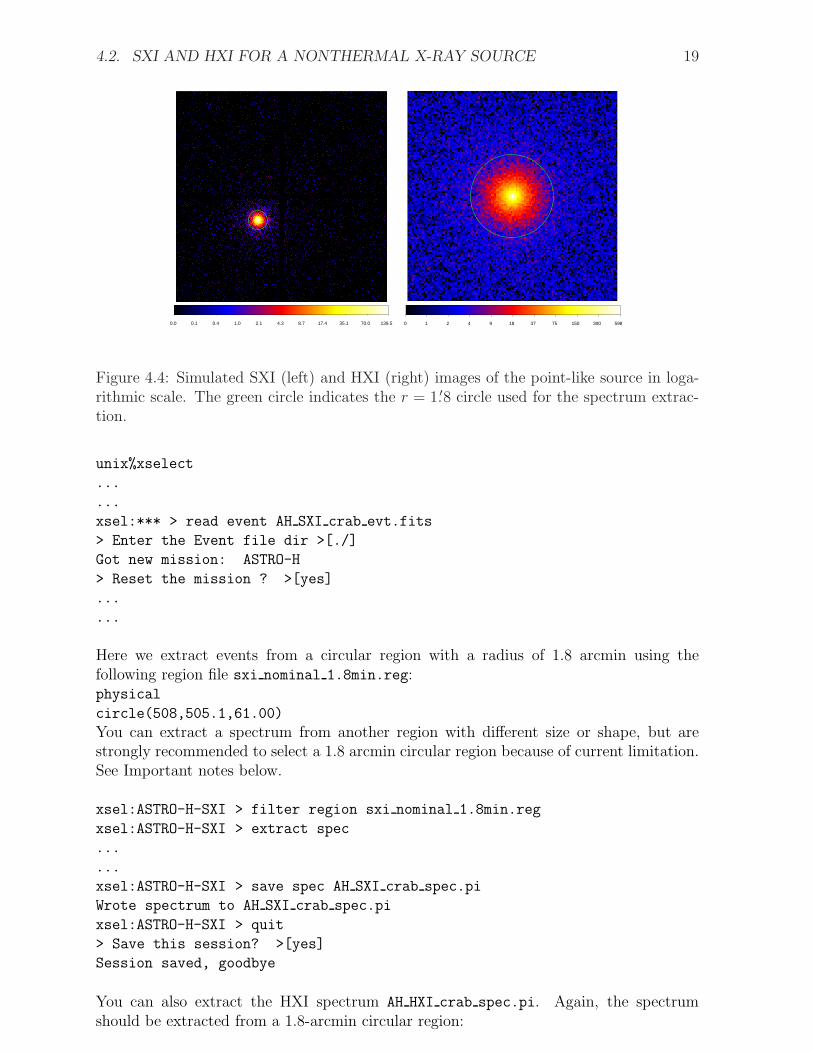
Images in the obtained event files can be viewed with ds9. The SXI and HXI images areshown in Figure 4.4 left and right, respectively. Run XSELECT to save the spectra.


0.0 0.1 0.4 1.0 2.1 4.3 8.7 17.4 35.1 70.0 139.5 0 1 2 4 9 18 37 75 150 300 598

Figure 4.4: Simulated SXI (left) and HXI (right) images of the point-like source in loga-rithmic scale. The green circle indicates the r = 1.′8 circle used for the spectrum extrac-tion.

unix%xselect

...

...

xsel:*** > read event AH SXI crab evt.fits




...

...

Here we extract events from a circular region with a radius of 1.8 arcmin using thefollowing region file sxi nominal 1.8min.reg:physical

circle(508,505.1,61.00)

You can extract a spectrum from another region with different size or shape, but arestrongly recommended to select a 1.8 arcmin circular region because of current limitation.See Important notes below.

xsel:ASTRO-H-SXI > filter region sxi nominal 1.8min.reg

xsel:ASTRO-H-SXI > extract spec

...

...

xsel:ASTRO-H-SXI > save spec AH SXI crab spec.pi

Wrote spectrum to AH SXI crab spec.pi

xsel:ASTRO-H-SXI > quit

> Save this session? >[yes]

Session saved, goodbye

You can also extract the HXI spectrum AH HXI crab spec.pi. Again, the spectrumshould be extracted from a 1.8-arcmin circular region:


physical

circle(64.5,64.5,25.1)

Important notes :

(1) Currently, the SXT/HXT team provides only the ARF data for point-like sources witha circular integration region with a radius of 1.8 arcmin. Thus, user should extract eventsfrom these regions to measure the source flux precisely.(2) You can simulate an off-axis source as well. Note, however, that the current versionof simx includes the PSF/EEF information only for the on-axis. Thus, the EEF of theoff-axis regions will always be under-estimated.

It would be useful to make links of the RMF, ARF, and NXB files in your work di-rectory.(For SXI)unix% ln -s /path/to/simx/inputs/Astro-H/response/SXI/

ah sxi 20120702.rmf .

unix% ln -s /path/to/simx/inputs/Astro-H/response/SXI/

sxt-i 140505 ts02um int01.8r.arf .

unix% ln -s /path/to/simx/inputs/Astro-H/bkgnd/SXI/

ah sxi pch nxb r1p80 20110530.pi . (for the 1.8-arcmin region)unix% ln -s /path/to/simx/inputs/Astro-H/bkgnd/SXI/

ah sxi pch nxb full 20110530.pi . (for the entire FoV)

(For HXI)unix% ln -s /path/to/simx/inputs/Astro-H/response/HXI/ah hxi 20090217.rmf .

unix% ln -s /path/to/simx/inputs/Astro-H/response/HXI/

ah hxt pnt r1p80 20130527.arf .

unix% ln -s /path/to/simx/inputs/Astro-H/bkgnd/HXI/

ah hxi nxb r6p3mm.pha . (for the 1.8-arcmin region)unix% ln -s /path/to/simx/inputs/Astro-H/bkgnd/HXI/

ah hxi nxb 30x30mm2.pha . (for the entire FoV)

Note that there are two different NXB files for both SXI and HXI: one for on-axis 1.8-arcmin regions and the other for the entire FoV. Since we have extracted the sourcespectra from the 1.8-arcmin regions, one may consider that the former NXB files shouldbe used for background subtraction. However, you should subtract the latter NXB fromthe source spectra. This is because both NXB files contain the BACKSCAL value of unity,while the extracted source spectra has the value of the ratio A/D, where A and D arethe area from which the spectrum is extracted) and the total detector area, respectively.For more detailed information of the BACKSCAL keyword, refer to the URLhttp://heasarc.gsfc.nasa.gov/docs/asca/abc backscal.html .Instead of this, you can modify the BACKSCAL keyword (using the fparkey command) byyourself as it matches the value of the source spectrum. On the other hand, you should usethe former NXB files for direct comparison of the source and NXB spectra, as performedin the following.

unix% grppha

Please enter PHA filename[] AH SXI crab spec.pi

Please enter output filename[] AH SXI crab spec grp.pi

GRPPHA[] gr min 100


1 10 100

10−

510

−4

10−

30.

010.

11

norm

aliz

ed c

ount

s s

−1

keV

−1

Energy (keV)

10−3

0.01

0.1

1

1 102 5 20

−4−2

024

Energy (keV)

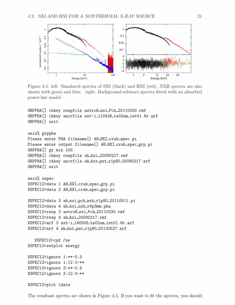
Figure 4.5: left: Simulated spectra of SXI (black) and HXI (red). NXB spectra are alsoshown with green and blue. right: Background-subtract spectra fitted with an absorbedpower-law model.

GRPPHA[] chkey respfile astroH sxi Pch 20110330.rmf

GRPPHA[] chkey ancrfile sxt-i 110426 ts02um int01.8r.arf

GRPPHA[] exit

unix% grppha

Please enter PHA filename[] AH HXI crab spec.pi

Please enter output filename[] AH HXI crab spec grp.pi

GRPPHA[] gr min 100

GRPPHA[] chkey respfile ah hxi 20090217.rmf

GRPPHA[] chkey ancrfile ah hxt pnt r1p80 20090217.arf

GRPPHA[] exit

unix% xspec

XSPEC12>data 1 AH SXI crab spec grp.pi

XSPEC12>data 2 AH HXI crab spec grp.pi

XSPEC12>data 3 ah sxi pch nxb r1p80 20110511.pi

XSPEC12>data 4 ah hxi nxb r6p3mm.pha

XSPEC12>resp 3 astroH sxi Pch 20110330.rmf

XSPEC12>resp 4 ah hxi 20090217.rmf

XSPEC12>arf 3 sxt-i 140505 ts02um int01.8r.arf

XSPEC12>arf 4 ah hxt pnt r1p80 20130527.arf

XSPEC12>cpd /xw


XSPEC12>ignore 1:**-0.5

XSPEC12>ignore 1:12.0-**

XSPEC12>ignore 3:**-0.5

XSPEC12>ignore 3:12.0-**

XSPEC12>plot ldata

The resultant spectra are shown in Figure 4.5. If you want to fit the spectra, you should


subtract the background. In this case, the NXB data from 1.8-arcmin region should beused for the reason mentioned above.

XSPEC12>back 1 ah sxi pch nxb full 20110530.pi

XSPEC12>back 2 ah hxi nxb 30x30mm2.pha

Important notes :

(1) The SXI (and SXS) NXB data currently include no instrumental-fluorescence-linecomponent, but only the continuum component.(2) The default output from simx does not include cosmic X-ray background (CXB), butonly the NXB. — In this chapter, we ignore contribution of CXB. The CXB data are needto be created by users separately. The method will be introduced in the next chapter.

Chapter 5

Tutorial 2: More Detailed Simulation

In the previous chapter, we learned how simx works for very simple cases. However, realobservations will often be more complicated; X-ray sources are extended, contributions ofdiffuse background components (i.e., CXB, LHB, etc.) are not negligible, multiple sourceswith different spectra are observed in one FoV. Here, we learn how to treat such complexsituation with simx.

5.1 Image mode

For simulation of specific diffuse sources, the option SourceImageType=Image can be used.This mode requires a surface brightness map in FITS format. Spatially-high-resolutionimages, such as ROSAT or Chandra observation data, are recommended as an input.

Some example images are available in the test/reference directory. Here, we use theChandra ACIS image of the supernova remnant Cas A (Figure 5.1(left)).

unix% ln -s /path/to/test/reference/casa.fits .

A spectral model for the energy band above 10 keV (the HXI band) is assumed to be apower-law with Γ = 3 and F10−100 keV = 1.3× 10−10 erg cm−2 s−1.

XSPEC12>model pow

1:powerlaw:PhoIndex>3

2:powerlaw:norm>1

XSPEC12> dummyrsp 10 100 900 linear

XSPEC12>plot model

XSPEC12>iplot

PLT>wenv model casa 10k-100k.qdp

Set simulation parameters and then run simx. The input flux should be that from theentire object. simx scatters input photons in accordance with the surface brightness map.

unix%pset simx OutputFileName=AH HXI casa

unix%pset simx PointingRA=350.86

unix%pset simx PointingDec=58.82


unix%pset simx SourceFlux=1.3e-10

24 CHAPTER 5. TUTORIAL 2: MORE DETAILED SIMULATION

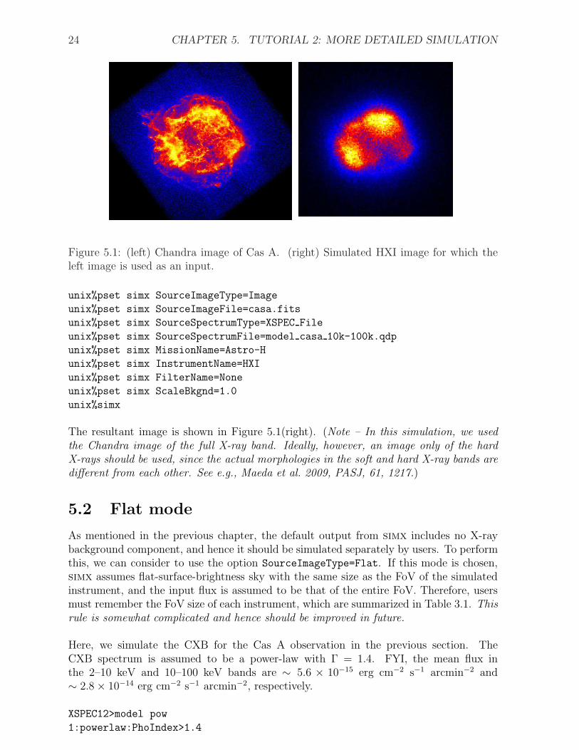
Figure 5.1: (left) Chandra image of Cas A. (right) Simulated HXI image for which theleft image is used as an input.

unix%pset simx SourceImageType=Image

unix%pset simx SourceImageFile=casa.fits


unix%pset simx SourceSpectrumFile=model casa 10k-100k.qdp





unix%simx

The resultant image is shown in Figure 5.1(right). (Note – In this simulation, we usedthe Chandra image of the full X-ray band. Ideally, however, an image only of the hardX-rays should be used, since the actual morphologies in the soft and hard X-ray bands aredifferent from each other. See e.g., Maeda et al. 2009, PASJ, 61, 1217.)

5.2 Flat mode

As mentioned in the previous chapter, the default output from simx includes no X-raybackground component, and hence it should be simulated separately by users. To performthis, we can consider to use the option SourceImageType=Flat. If this mode is chosen,simx assumes flat-surface-brightness sky with the same size as the FoV of the simulatedinstrument, and the input flux is assumed to be that of the entire FoV. Therefore, usersmust remember the FoV size of each instrument, which are summarized in Table 3.1. Thisrule is somewhat complicated and hence should be improved in future.

Here, we simulate the CXB for the Cas A observation in the previous section. TheCXB spectrum is assumed to be a power-law with Γ = 1.4. FYI, the mean flux inthe 2–10 keV and 10–100 keV bands are ∼ 5.6 × 10−15 erg cm−2 s−1 arcmin−2 and∼ 2.8× 10−14 erg cm−2 s−1 arcmin−2, respectively.

XSPEC12>model pow


5.2. FLAT MODE 25

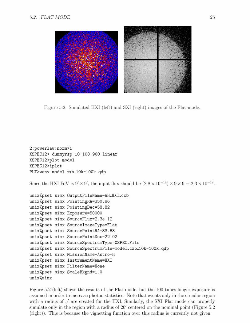
Figure 5.2: Simulated HXI (left) and SXI (right) images of the Flat mode.

2:powerlaw:norm>1

XSPEC12> dummyrsp 10 100 900 linear

XSPEC12>plot model

XSPEC12>iplot

PLT>wenv model cxb 10k-100k.qdp

Since the HXI FoV is 9′ × 9′, the input flux should be (2.8× 10−14)× 9× 9 = 2.3× 10−12.

unix%pset simx OutputFileName=AH HXI cxb

unix%pset simx PointingRA=350.86

unix%pset simx PointingDec=58.82


unix%pset simx SourceFlux=2.3e-12

unix%pset simx SourceImageType=Flat




unix%pset simx SourceSpectrumFile=model cxb 10k-100k.qdp





unix%simx

Figure 5.2 (left) shows the results of the Flat mode, but the 100-times-longer exposure isassumed in order to increase photon statistics. Note that events only in the circular regionwith a radius of 5′ are created for the HXI. Similarly, the SXI Flat mode can properlysimulate only in the region with a radius of 20′ centered on the nominal point (Figure 5.2(right)). This is because the vignetting function over this radius is currently not given.


5.3 Merging multiple event data

The event data frommultiple simx simulation can be merged together using the simxmergeutility. Here, we merge the Cas A and CXB data created in the previous sections.

Important note : simxmerge should not be used to merge event files from any othersource besides simx.

unix%pset simxmerge OutputFileName=merged

unix%pset simxmerge MergeFiles=AH HXI casa evt.fits,AH HXI cxb evt.fits

unix%simxmerge

Then, you will obtain the merged event data merged evt.fits. You can, of course,merge multiple sources in the same FoV with different spectra using this utility.

5.4 Application for clusters of galaxies

In this section, we demonstrate simulations for a cluster of glaxies, which is charactrizedby the diffuse emission and variation of the spectral shape in regions of the cluster.We pick up Abell 2199 clsuter. The cluster is a nearby and bright cluster of galaxies(z = 0.03) characterized by a smooth distribution of the intra-cluster medium (ICM).Recent Chandra, XMM-Newton and Suzaku observations show the ICM properties fromthe central to outer region of the cluster (e.g., Sanders & Fabian 2006, Snowden et al.2008, Kawaharada et al. 2010).

5.4.1 Preparation for simulations

We need several information for simulations, such as the temperature, flux, surface bright-ness profiles, etc. Fundamental parameters of Abell 2199 for simulations are summarizedin table 5.1.

Table 5.1: Fundamental parameters of Abell 2199 cluster.(R.A., Dec.) z NH β∗ r∗

c

(degree) (cm−2) kpc(247.1604, +39.5517) 0.03 8.92×1019 0.650/0.531 10.3/51.0

r < 1.5′ 1.5′ < r < 4.5′ 4.5′ < r < 7.5′ 7.5′ < r < 10.5′

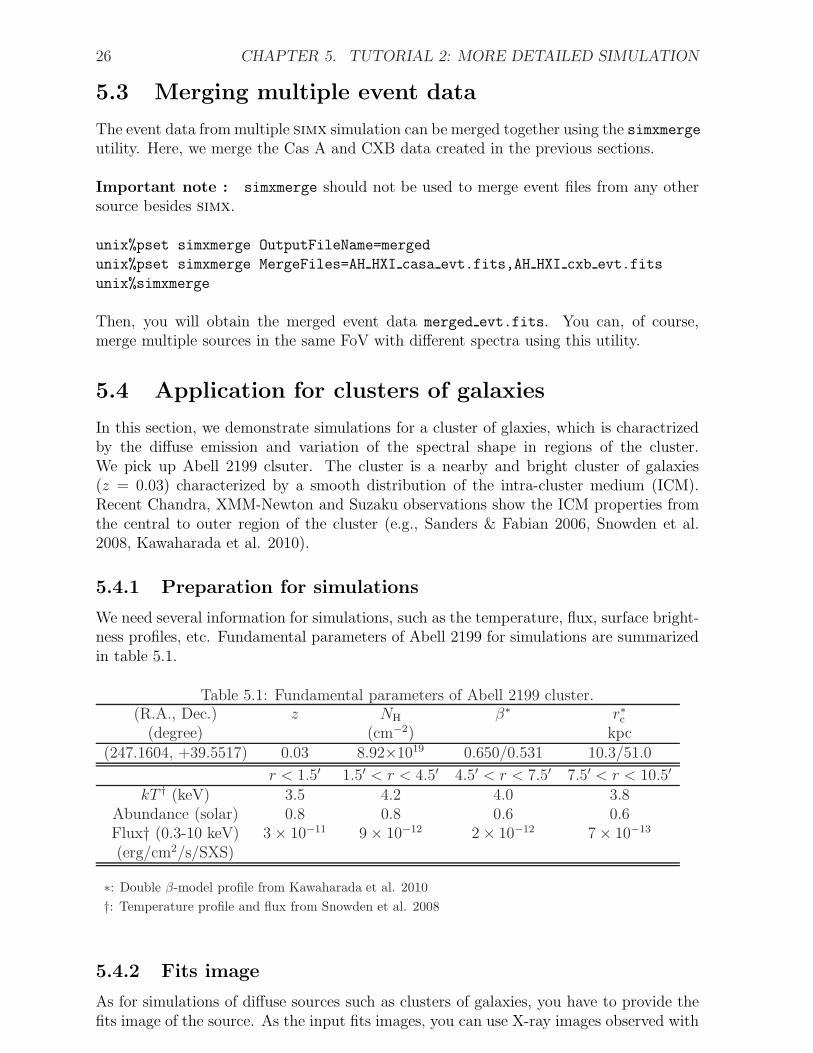
kT † (keV) 3.5 4.2 4.0 3.8Abundance (solar) 0.8 0.8 0.6 0.6Flux† (0.3-10 keV) 3× 10−11 9× 10−12 2× 10−12 7× 10−13

(erg/cm2/s/SXS)

∗: Double β-model profile from Kawaharada et al. 2010

†: Temperature profile and flux from Snowden et al. 2008

5.4.2 Fits image

As for simulations of diffuse sources such as clusters of galaxies, you have to provide thefits image of the source. As the input fits images, you can use X-ray images observed with

5.4. APPLICATION FOR CLUSTERS OF GALAXIES 27

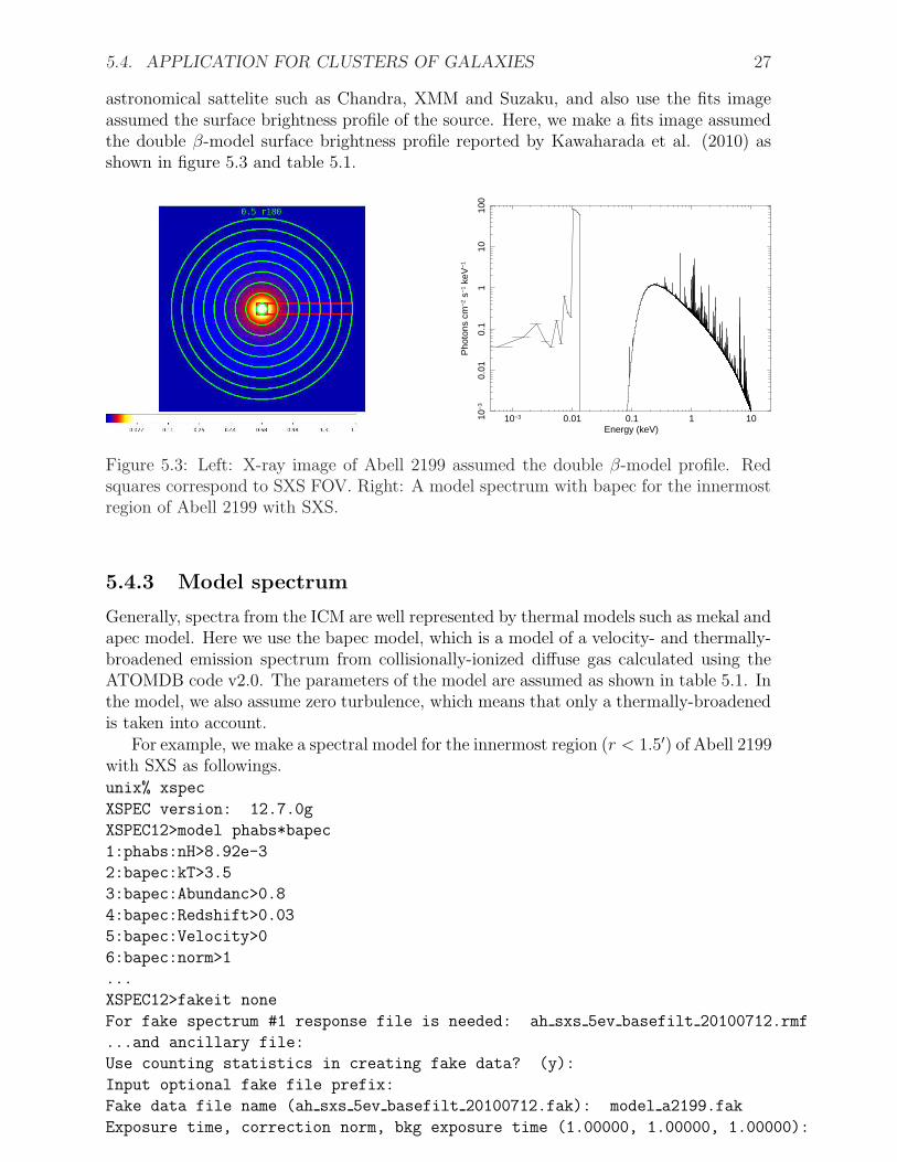
astronomical sattelite such as Chandra, XMM and Suzaku, and also use the fits imageassumed the surface brightness profile of the source. Here, we make a fits image assumedthe double β-model surface brightness profile reported by Kawaharada et al. (2010) asshown in figure 5.3 and table 5.1.

10−3 0.01 0.1 1 1010−

30.

010.

11

1010

0

Pho

tons

cm

−2

s−1

keV

−1

Energy (keV)

Figure 5.3: Left: X-ray image of Abell 2199 assumed the double β-model profile. Redsquares correspond to SXS FOV. Right: A model spectrum with bapec for the innermostregion of Abell 2199 with SXS.

5.4.3 Model spectrum

Generally, spectra from the ICM are well represented by thermal models such as mekal andapec model. Here we use the bapec model, which is a model of a velocity- and thermally-broadened emission spectrum from collisionally-ionized diffuse gas calculated using theATOMDB code v2.0. The parameters of the model are assumed as shown in table 5.1. Inthe model, we also assume zero turbulence, which means that only a thermally-broadenedis taken into account.

For example, we make a spectral model for the innermost region (r < 1.5′) of Abell 2199with SXS as followings.unix% xspec

XSPEC version: 12.7.0g

XSPEC12>model phabs*bapec

1:phabs:nH>8.92e-3

2:bapec:kT>3.5

3:bapec:Abundanc>0.8

4:bapec:Redshift>0.03

5:bapec:Velocity>0

6:bapec:norm>1

...

XSPEC12>fakeit none

For fake spectrum #1 response file is needed: ah sxs 5ev basefilt 20100712.rmf

...and ancillary file:

Use counting statistics in creating fake data? (y):

Input optional fake file prefix:

Fake data file name (ah sxs 5ev basefilt 20100712.fak): model a2199.fak

Exposure time, correction norm, bkg exposure time (1.00000, 1.00000, 1.00000):



XSPEC12>plot model

XSPEC12>iplot

PLT>wenv model bapec a2199

PLT>quit

XSPEC12>quit

5.4.4 Running simx

Using the above model and paramaters, you can now run simx for SXS. You can alsosimulate event files for SXI by the same way. The resultant simulated SXS/SXI imagesare shown in figure 5.4.

pset simx OutputFileName=AH SXS a2199 cen

pset simx PointingRA=247.1604

pset simx PointingDec=39.5517

pset simx Exposure=50000

pset simx SourceFlux=3.2e-11

pset simx SourceImageType=Image

pset simx SourcePointRA=247.1604

pset simx SourcePointDec=39.5517

pset simx SourceImageFile=a2199-2beta reg1.fits

pset simx SourceSpectrumType=XSPEC File

pset simx SourceSpectrumFile=model bapec a2199.qdp

pset simx MissionName=Astro-H

pset simx InstrumentName=SXS

pset simx FilterName=None

unix% simx

**************************


**************************

Output Event file stem[AH SXS a2199 reg1]




Use Simput File for source definition?[no]

Source Flux in erg/cm^2/s[3.2e-11]

Source Image Type (Point|Flat|Image) [Image]



Source Image File[a2199-2beta.fits]

Source Spectrum Type (XSPEC File|Sherpa File|Mono) [XSPEC File]

Source Spectrum File[model bapec a2199.qdp]

Energy (in keV) if monoenergetic[1.0]



Instrument Name[SXS]

Filter Name[None]





generate events: Analyzing deadtime and pileup


generate events: Best-resolution events : 93424 ( 98.77%)

generate events: Mid-resolution events : 878 ( 0.93%)

generate events: Low-resolution events : 287 ( 0.30%)

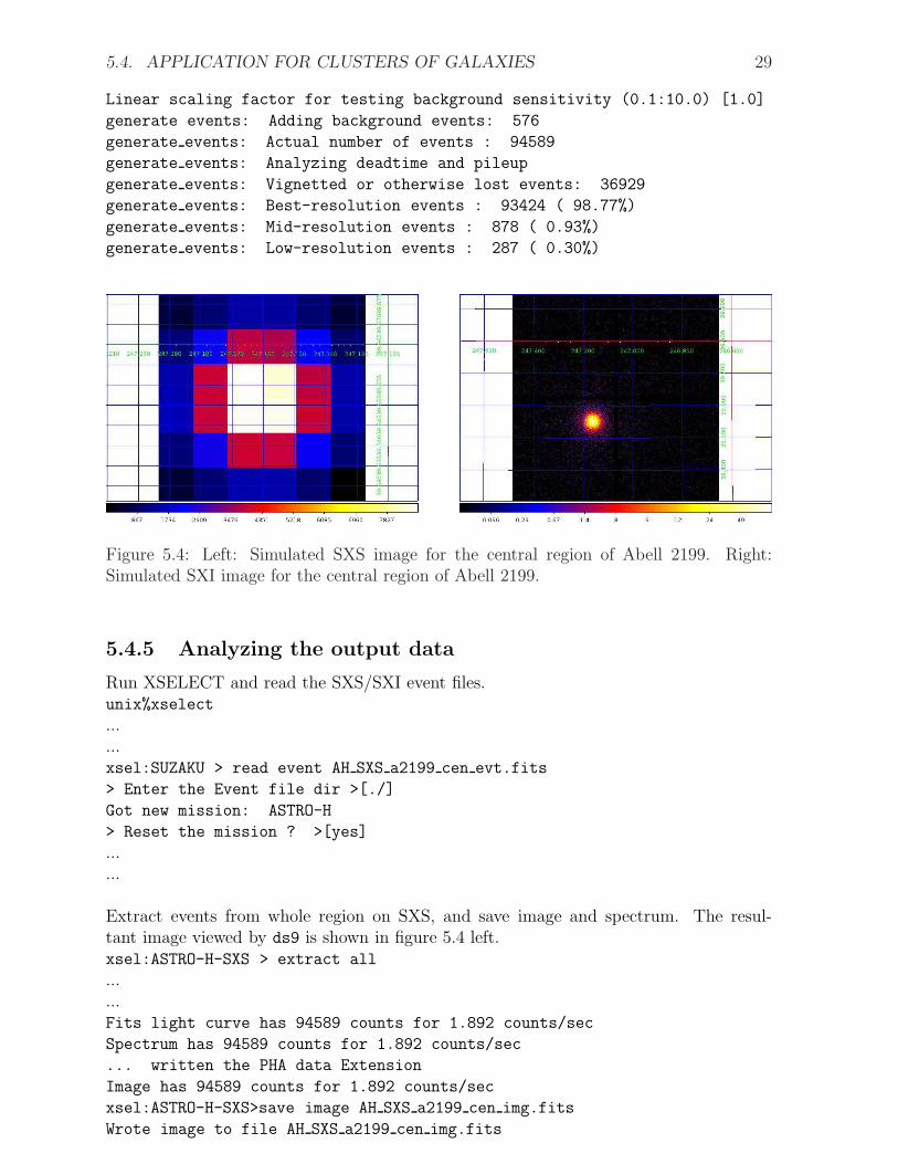
Figure 5.4: Left: Simulated SXS image for the central region of Abell 2199. Right:Simulated SXI image for the central region of Abell 2199.

5.4.5 Analyzing the output data

Run XSELECT and read the SXS/SXI event files.unix%xselect

...

...xsel:SUZAKU > read event AH SXS a2199 cen evt.fits




...

...

Extract events from whole region on SXS, and save image and spectrum. The resul-tant image viewed by ds9 is shown in figure 5.4 left.xsel:ASTRO-H-SXS > extract all

...

...Fits light curve has 94589 counts for 1.892 counts/sec

Spectrum has 94589 counts for 1.892 counts/sec

... written the PHA data Extension

Image has 94589 counts for 1.892 counts/sec

xsel:ASTRO-H-SXS>save image AH SXS a2199 cen img.fits

Wrote image to file AH SXS a2199 cen img.fits


xsel:ASTRO-H-SXS>save spec AH SXS a2199 cen spec.pi

Wrote spectrum to AH SXS a2199 cen spec.pi

xsel:ASTRO-H-SXS>quit

> Save this session? >[no]

The spectrum can be viewed and analyzed with xspec. For the analysis, it is usefulto link the ancillary response files (arf) and non X-ray background (NXB) files to yourdirectory.


ah sxs 5ev basefilt 20100712.rmf .


sxt-s 100208 ts02um of intallpxl.arf .

unix% ln -s /path/to/simx/inputs/Astro-H/bkgnd/SXS/

sxs-bck 20100219 1Gs.pha .

(For SXI)


astroH sxi Pch 20110330.rmf .


sxt-i 110426 ts02um int01.8r.arf .

unix% ln -s /path/to/simx/inputs/Astro-H/bkgnd/SXI/

ah sxi pch nxb r1p80 20110511.pi .

unix% xspec

XSPEC version: 12.7.0g

...XSPEC12>data 1 spec AH SXS a2199 cen spec.pi

XSPEC12>response 1 ah sxs 5ev basefilt 20100712.rmf

XSPEC12>arf 1 sxt-s 100208 ts02um intallpxl.arf

XSPEC12>backgrnd 1 sxs-bck 20100219 1Gs.pha

XSPEC12>cpd /xw


XSPEC12>ignore *:**-0.3

XSPEC12>ignore *:8.0-**

XSPEC12>setplot rebin 10 50

XSPEC12>plot ldata

The resultant spectrum is shown in figure 5.5.

5.4.6 background estimations

For the ICM measurement in lower surface brightness resions of clusters, especially forouter region of clusters, estimations of fore- and background, the Galactic and cosmic X-


10.5 2 5

10−

410

−3

0.01

0.1

1

norm

aliz

ed c

ount

s s−

1 ke

V−

1

Energy (keV)10.5 2 5

10−

410

−3

0.01

0.1

1

norm

aliz

ed c

ount

s s−

1 ke

V−

1

Energy (keV)

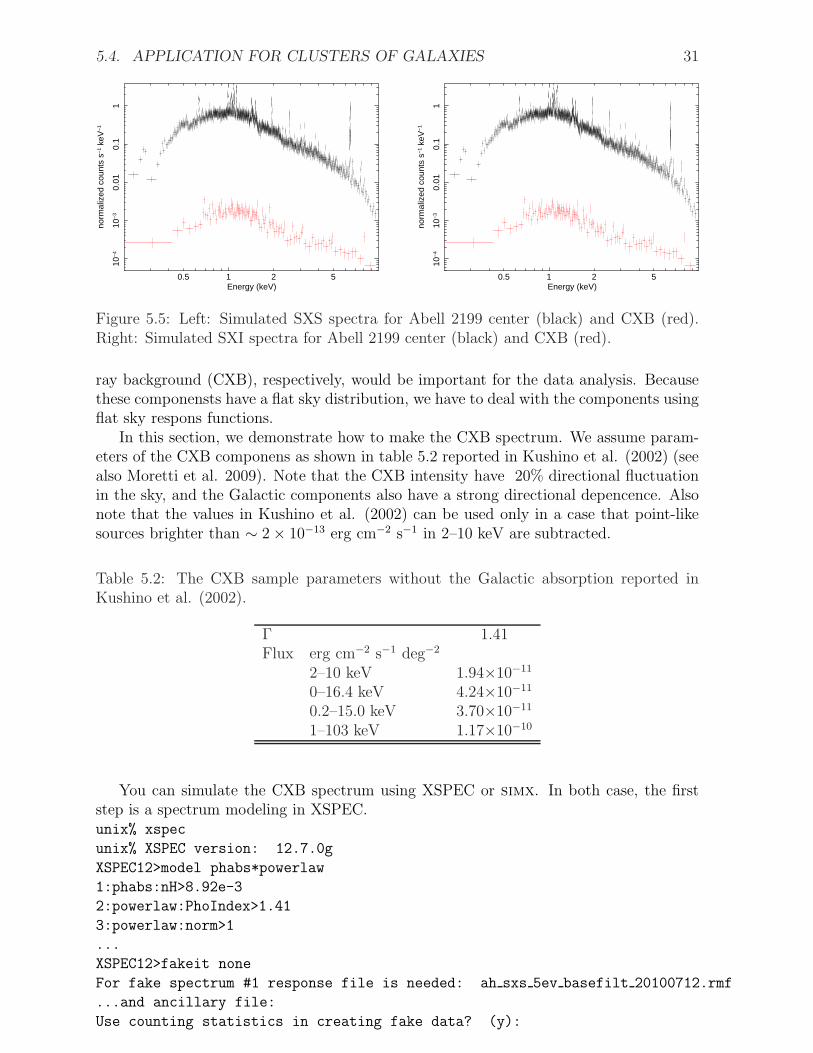
Figure 5.5: Left: Simulated SXS spectra for Abell 2199 center (black) and CXB (red).Right: Simulated SXI spectra for Abell 2199 center (black) and CXB (red).

ray background (CXB), respectively, would be important for the data analysis. Becausethese componensts have a flat sky distribution, we have to deal with the components usingflat sky respons functions.

In this section, we demonstrate how to make the CXB spectrum. We assume param-eters of the CXB componens as shown in table 5.2 reported in Kushino et al. (2002) (seealso Moretti et al. 2009). Note that the CXB intensity have 20% directional fluctuationin the sky, and the Galactic components also have a strong directional depencence. Alsonote that the values in Kushino et al. (2002) can be used only in a case that point-likesources brighter than ∼ 2× 10−13 erg cm−2 s−1 in 2–10 keV are subtracted.

Table 5.2: The CXB sample parameters without the Galactic absorption reported inKushino et al. (2002).

Γ 1.41Flux erg cm−2 s−1 deg−2

2–10 keV 1.94×10−11

0–16.4 keV 4.24×10−11

0.2–15.0 keV 3.70×10−11

1–103 keV 1.17×10−10

You can simulate the CXB spectrum using XSPEC or simx. In both case, the firststep is a spectrum modeling in XSPEC.unix% xspec

unix% XSPEC version: 12.7.0g

XSPEC12>model phabs*powerlaw

1:phabs:nH>8.92e-3


3:powerlaw:norm>1

...

XSPEC12>fakeit none

For fake spectrum #1 response file is needed: ah sxs 5ev basefilt 20100712.rmf

...and ancillary file:

Use counting statistics in creating fake data? (y):


Input optional fake file prefix:

Fake data file name (ah sxs 5ev basefilt 20100712.fak): cxb sxs.fak

Exposure time, correction norm, bkg exposure time (1.00000, 1.00000, 1.00000):

XSPEC12>plot model

XSPEC12>iplot

PLT> wenv cxb sxs model

Chapter 6

Tutorial 3: A Point Source with Full

PSF Information

6.1 SXI for a monochromatic X-ray source

In this section, we learn how to run simx assuming a virtual point-like source with asimple monoenergetic spectrum, but also using the full 2-D point spread function. Thisrequires the at least version 2.1.0 of simx. Hereafter, users are assumed to use this version.

Running simx

As this is simply a monoenergetic spectrum, the run can be done directly in simx. How-ever, you can set the input parameter before simx is executed. (This process can beskipped, if you prefer to input the parameters interactively after running simx.)

Set the stem of the output event file name.unix%pset simx OutputFileName=AH SXIPSF point 2kev

(The file name will be this with ” evt.fits” appended.)

Set the pointing position.unix%pset simx PointingRA = 0.0


Set the exposure (in sec).unix%pset simx Exposure=100000

Set the flux (in erg/cm−2/s).unix%pset simx SourceFlux=5e-11

Set the input image or pointing position. (Here we simulate a point-like source. Thereare other options, Flat and Image, which will be explained in the next chapter.)unix%pset simx SourceImageType=Point




Set the input spectrum.unix%pset simx SourceSpectrumType=Mono

34CHAPTER 6. TUTORIAL 3: A POINT SOURCEWITH FULL PSF INFORMATION

unix%pset simx MonoEnergy=2.0

Set the mission/instrument/filter names.unix%pset simx MissionName=Astro-H

unix%pset simx InstrumentName=SXIPSF


Set the linear scaling factor of the background level. The available range is from 0.0 to10.0. (This option is useful to investigate impact of change in the background level.)Here we simply use the default background. unix%pset simx ScaleBkgnd=1.0

Finally, run simx to create an event file AH SXI point 2kev evt.fits. Do not forget setupsimx:


unix%simx

**************************


**************************

Output Event file stem[AH SXIPSF point 2kev]




Source Flux in erg/cm2/s[5e-11]

Source Image Type (Point|Flat|Image) [Point]



Source Image File[None]

Source Spectrum Type (XSPEC File|Sherpa File|Mono) [Mono]

Energy (in keV) if monoenergetic[2.0]



Instrument Name[SXI]

Filter Name[None]


...

...

...

initialize: Approximate # of source counts : 742246

generate events: Progress: |..................................................|

read PSF image: Number of PSF image in file: 1

read PSF image: Reading HDU 1

...



...

...

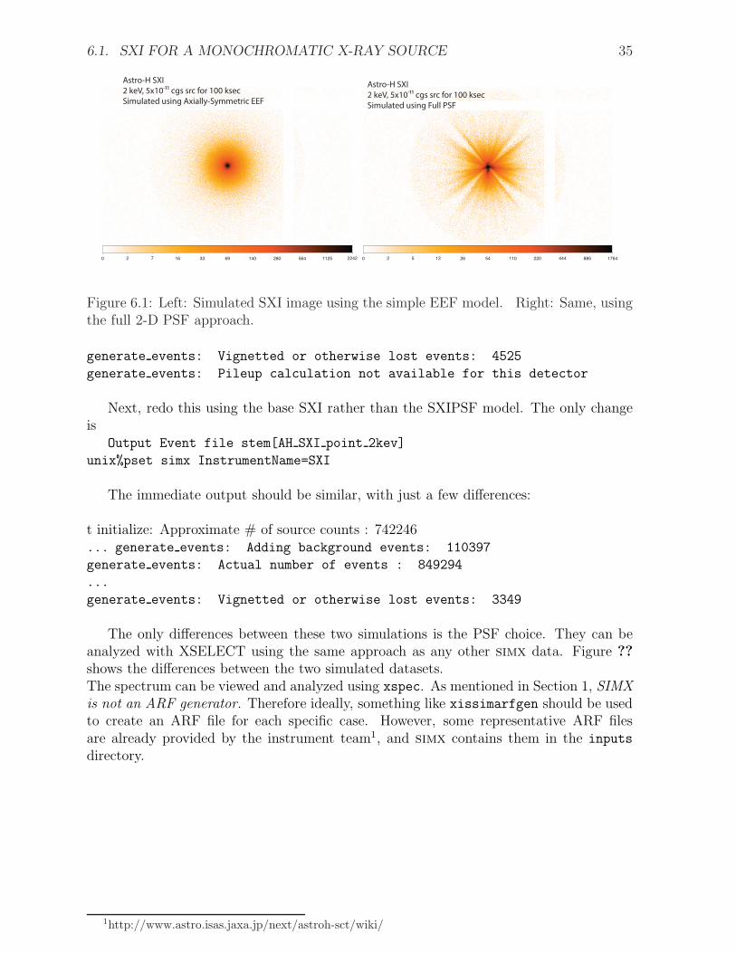
6.1. SXI FOR A MONOCHROMATIC X-RAY SOURCE 35

0 2 7 16 33 69 140 280 564 1125 2242

Astro-H SXI2 keV, 5x10-11 cgs src for 100 ksec Simulated using Axially-Symmetric EEF

0 2 5 12 26 54 110 220 444 885 1764

Astro-H SXI2 keV, 5x10-11 cgs src for 100 ksec Simulated using Full PSF

Figure 6.1: Left: Simulated SXI image using the simple EEF model. Right: Same, usingthe full 2-D PSF approach.


generate events: Pileup calculation not available for this detector

Next, redo this using the base SXI rather than the SXIPSF model. The only changeis

Output Event file stem[AH SXI point 2kev]

unix%pset simx InstrumentName=SXI

The immediate output should be similar, with just a few differences:

t initialize: Approximate # of source counts : 742246... generate events: Adding background events: 110397


...


The only differences between these two simulations is the PSF choice. They can beanalyzed with XSELECT using the same approach as any other simx data. Figure ??

shows the differences between the two simulated datasets.The spectrum can be viewed and analyzed using xspec. As mentioned in Section 1, SIMXis not an ARF generator. Therefore ideally, something like xissimarfgen should be usedto create an ARF file for each specific case. However, some representative ARF filesare already provided by the instrument team1, and simx contains them in the inputs

directory.

1http://www.astro.isas.jaxa.jp/next/astroh-sct/wiki/

Chapter 7

Brief Overview of “SIMX”

Calculations

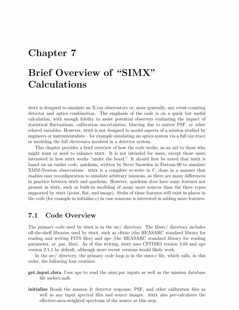
simx is designed to simulate an X-ray observatory or, more generally, any event-countingdetector and optics combination. The emphasis of the code is on a quick but usefulcalculation, with enough fidelity to assist potential observers evaluating the impact ofstatistical fluctuations, calibration uncertainties, blurring due to mirror PSF, or otherrelated variables. However, simx is not designed to model aspects of a mission studied byengineers or instrumentalists – for example simulating an optics system via a full ray-traceor modeling the full electronics involved in a detector system.

This chapter provides a brief overview of how the code works, as an aid to those whomight want or need to enhance simx. It is not intended for users, except those usersinterested in how simx works “under the hood.” It should first be noted that simx isbased on an earlier code, quicksim, written by Steve Snowden in Fortran-90 to simulateXMM-Newton observations. simx is a complete re-write in C, done in a manner thatenables easy reconfiguration to simulate arbitrary missions, so there are many differencesin practice between simx and quicksim. However, quicksim does have some features notpresent in simx, such as built-in modeling of many more sources than the three typessupported by simx (point, flat, and image). Stubs of these features still exist in places inthe code (for example in initialize.c) in case someone is interested in adding more features.

7.1 Code Overview

The primary code used by simx is in the src/ directory. The libsrc/ directory includesoff-the-shelf libraries used by simx, such as cfitsio (the HEASARC standard library forreading and writing FITS files) and ape (the HEASARC standard library for readingparameter, or .par, files). As of this writing, simx uses CFITSIO version 3.03 and apeversion 2.1.1 by default, although more recent versions would likely work.

In the src/ directory, the primary code loop is in the simx.c file, which calls, in thisorder, the following four routines:

get input data Uses ape to read the simx.par inputs as well as the mission databasefile xselect.mdb

initialize Reads the mission & detector response, PSF, and other calibration files aswell as any input spectral files and source images. simx also pre-calculates theeffective-area-weighted spectrum of the source at this step.

7.2. DATA STRUCTURES OVERVIEW 37

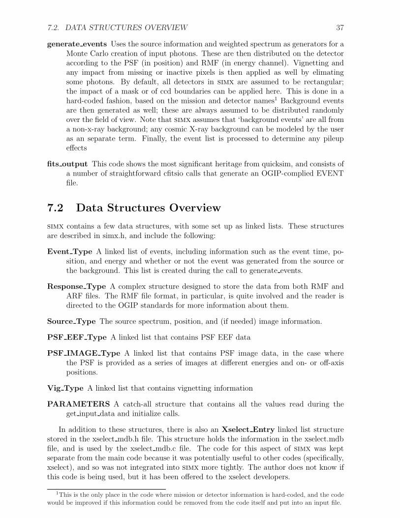
generate events Uses the source information and weighted spectrum as generators for aMonte Carlo creation of input photons. These are then distributed on the detectoraccording to the PSF (in position) and RMF (in energy channel). Vignetting andany impact from missing or inactive pixels is then applied as well by elimatingsome photons. By default, all detectors in simx are assumed to be rectangular;the impact of a mask or of ccd boundaries can be applied here. This is done in ahard-coded fashion, based on the mission and detector names1 Background eventsare then generated as well; these are always assumed to be distributed randomlyover the field of view. Note that simx assumes that ‘background events’ are all froma non-x-ray background; any cosmic X-ray background can be modeled by the useras an separate term. Finally, the event list is processed to determine any pileupeffects

fits output This code shows the most significant heritage from quicksim, and consists ofa number of straightforward cfitsio calls that generate an OGIP-complied EVENTfile.

7.2 Data Structures Overview

simx contains a few data structures, with some set up as linked lists. These structuresare described in simx.h, and include the following:

Event Type A linked list of events, including information such as the event time, po-sition, and energy and whether or not the event was generated from the source orthe background. This list is created during the call to generate events.

Response Type A complex structure designed to store the data from both RMF andARF files. The RMF file format, in particular, is quite involved and the reader isdirected to the OGIP standards for more information about them.

Source Type The source spectrum, position, and (if needed) image information.

PSF EEF Type A linked list that contains PSF EEF data

PSF IMAGE Type A linked list that contains PSF image data, in the case wherethe PSF is provided as a series of images at different energies and on- or off-axispositions.

Vig Type A linked list that contains vignetting information

PARAMETERS A catch-all structure that contains all the values read during theget input data and initialize calls.

In addition to these structures, there is also an Xselect Entry linked list structurestored in the xselect mdb.h file. This structure holds the information in the xselect.mdbfile, and is used by the xselect mdb.c file. The code for this aspect of simx was keptseparate from the main code because it was potentially useful to other codes (specifically,xselect), and so was not integrated into simx more tightly. The author does not know ifthis code is being used, but it has been offered to the xselect developers.

1This is the only place in the code where mission or detector information is hard-coded, and the codewould be improved if this information could be removed from the code itself and put into an input file.

Chapter 8

Remarks

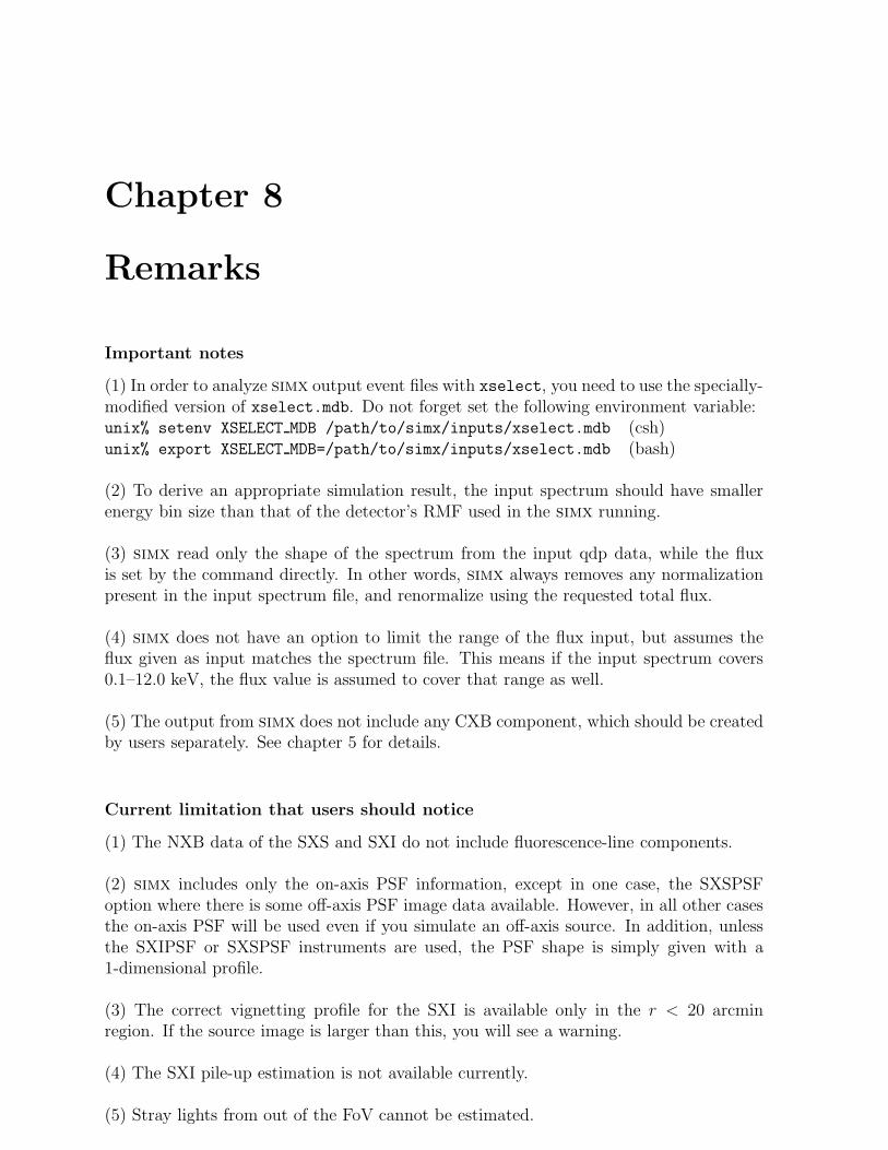
Important notes

(1) In order to analyze simx output event files with xselect, you need to use the specially-modified version of xselect.mdb. Do not forget set the following environment variable:unix% setenv XSELECT MDB /path/to/simx/inputs/xselect.mdb (csh)unix% export XSELECT MDB=/path/to/simx/inputs/xselect.mdb (bash)

(2) To derive an appropriate simulation result, the input spectrum should have smallerenergy bin size than that of the detector’s RMF used in the simx running.

(3) simx read only the shape of the spectrum from the input qdp data, while the fluxis set by the command directly. In other words, simx always removes any normalizationpresent in the input spectrum file, and renormalize using the requested total flux.

(4) simx does not have an option to limit the range of the flux input, but assumes theflux given as input matches the spectrum file. This means if the input spectrum covers0.1–12.0 keV, the flux value is assumed to cover that range as well.

(5) The output from simx does not include any CXB component, which should be createdby users separately. See chapter 5 for details.

Current limitation that users should notice

(1) The NXB data of the SXS and SXI do not include fluorescence-line components.

(2) simx includes only the on-axis PSF information, except in one case, the SXSPSFoption where there is some off-axis PSF image data available. However, in all other casesthe on-axis PSF will be used even if you simulate an off-axis source. In addition, unlessthe SXIPSF or SXSPSF instruments are used, the PSF shape is simply given with a1-dimensional profile.

(3) The correct vignetting profile for the SXI is available only in the r < 20 arcminregion. If the source image is larger than this, you will see a warning.

(4) The SXI pile-up estimation is not available currently.

(5) Stray lights from out of the FoV cannot be estimated.

39

(6) Out-of-time events cannot be estimated.

Documents

SIMXManual - Harvard Universityhea- · SIMXManual for ASTRO-H members ... (Center for Astrophysics) ... simxhome page at CfA