Single Image Dehazing

Raanan Fattal∗Hebrew University of Jerusalem, Israel

Input Output Depth

Figure 1: Dehazing based on a single input image and the corresponding depth estimate.

Abstract

In this paper we present a new method for estimating the opticaltransmission in hazy scenes given a single input image. Based onthis estimation, the scattered light is eliminated to increase scenevisibility and recover haze-free scene contrasts. In this new ap-proach we formulate a refined image formation model that accountsfor surface shading in addition to the transmission function. Thisallows us to resolve ambiguities in the data by searching for a solu-tion in which the resulting shading and transmission functions arelocally statistically uncorrelated. A similar principle is used to es-timate the color of the haze. Results demonstrate the new methodabilities to remove the haze layer as well as provide a reliable trans-mission estimate which can be used for additional applications suchas image refocusing and novel view synthesis.

CR Categories: I.3.3 [Computer Graphics]: Picture/ImageGeneration—Display algorithms; I.4.1 [Image Processing andComputer Vision]: Digitization and Image Capture—Radiometry

Keywords: image dehazing/defogging, computational photogra-phy, image restoration, image enhancement, Markov random fieldimage modeling

1 Introduction

In almost every practical scenario the light reflected from a surfaceis scattered in the atmosphere before it reaches the camera. This

∗e-mail: raananf@cs.huji.ac.il

is due to the presence of aerosols such as dust, mist, and fumeswhich deflect light from its original course of propagation. In longdistance photography or foggy scenes, this process has a substan-tial effect on the image in which contrasts are reduced and surfacecolors become faint. Such degraded photographs often lack visualvividness and appeal, and moreover, they offer a poor visibility ofthe scene contents. This effect may be an annoyance to amateur,commercial, and artistic photographers as well as undermine thequality of underwater and aerial photography. This may also be thecase for satellite imaging which is used for many purposes includ-ing cartography and web mapping, land-use planning, archeology,and environmental studies.

As we shall describe shortly in more detail, in this processlight, which should have propagated in straight lines, is scat-tered and replaced by previously scattered light, called theairlight [Koschmieder 1924]. This results in a multiplicative lossof image contrasts as well as an additive term due to this uniformlight. In Section 3 we describe the model that is commonly usedto formalize the image formation in the presence of haze. In thismodel, the degraded image is factored into a sum of two compo-nents: the airlight contribution and the unknown surface radiance.Algebraically these two, three-channel color vectors, are convexlycombined by the transmission coefficient which is a scalar speci-fying the visibility at each pixel. Recovering a haze-free image re-quires us to determine the three surface color values as well as thetransmission value at every pixel. Since the input image provides usthree equations per pixel, the system is ambiguous and we cannotdetermine the transmission values. In Section 3 we give a formaldescription of this ambiguity, but intuitively it follows from our in-ability to answer the following question based on a single image:are we looking at a deep red surface through a thick white medium,or is it a faint red surface seen at a close range or through a clearmedium. In the general case this ambiguity, which we refer to asthe airlight-albedo ambiguity, holds for every pixel and can not beresolved independently at each pixel given a single input image.

In this paper we present a new method for recovering a haze-freeimage given a single photograph as an input. We achieve this byinterpreting the image through a model that accounts for surfaceshading in addition to the scene transmission. Based on this re-fined image formation model, the image is broken into regions of aconstant albedo and the airlight-albedo ambiguity is resolved by de-

riving an additional constraint that requires the surface shading andmedium transmission functions to be locally statistically uncorre-lated. This requires the shading component to vary significantlycompared to the noise present in the image. We use a graphicalmodel to propagate the solution to pixels in which the signal-to-noise ratio falls below an admissible level that we derive analyti-cally in the Appendix. The airlight color is also estimated usingthis uncorrelation principle. This new method is passive; it does notrequire multiple images of the scene, any light-blocking based po-larization, any form of scene depth information, or any specializedsensors or hardware. The new method has the minimal requirementof a single image acquired by an ordinary consumer camera. Alsoit does not assume the haze layer to be smooth in space, i.e., dis-continuities in the scene depth or medium thickness are permitted.As shown in Figure 1, despite the challenges this problem poses,this new method achieves a significant reduction of the airlight andrestores the contrasts of complex scenes. Based on the recoveredtransmission values we can estimate scene depths and use them forother applications that we describe in the Section 8.

This papers is organized as follows. We begin by reviewing existingworks on image restoration and haze removal. In Section 3 wepresent the image degradation model due to the presence of hazein the scene, and in Section 4 we present the core idea behind ournew approach for the restricted case of images consisting of a singlealbedo. We then extend our solution to images with multi-albedosurfaces in Section 6, and report the results in Section 8 as well ascompare it with alternative methods. In Section 9 we summarizeour approach and discuss its limitations.

2 Previous Work

In the context of computational photography there is an increasingfocus on developing methods that restore images as well as extract-ing other quantities at minimal requirements in terms of input data,user intervention, and sophistication of the acquisition hardware.Examples are recovery of an all-focus image and depth map using asimple modification to the camera’s aperture in [Levin et al. 2007].A similar modification is used in [Veeraraghavan et al. 2007] to re-construct the 4D light field of a scene from a 2D camera. Given twoimages, one noisy and the other blurry, a deblurring method witha reduced amount of ringing artifacts is described in [Yuan et al.2007]. Resolution enhancement with native-resolution edge sharp-ness based on a single input image is described in [Fattal 2007].In [Liu et al. 2006] intensity-dependent noise levels are estimatedfrom a single image using Bayesian inference.

Image dehazing is a very challenging problem and most of the pa-pers addressing it assume some form of additional data on top of thedegraded photograph itself. In [Tan and Oakley 2000] assuming thescene depth is given, atmospheric effects are removed from terrainimages taken by a forward-looking airborne camera. In [Schech-ner et al. 2001] polarized haze effects are removed given two pho-tographs. The camera must be identically positioned in the sceneand an attached polarization filter is set to a different angle for eachphotograph. This gives images that differ only in the magnitudeof the polarized haze light component. Using some estimate forthe degree of polarization, a parameter describing this difference inmagnitudes, the polarized haze light is removed. In [Shwartz et al.2006] this parameter is estimated automatically by assuming thatthe higher spatial-bands of the direct transmission, the surface radi-ance reaching the camera, and the polarized haze contribution areuncorrelated. We use a similar but more refined principle to sepa-rate the image into different components. These methods removethe polarized component of the haze light and provide impressiveresults. However in situations of fog or dense haze the polarizedlight is not the major source of the degradation and may also be tooweak as to undermine the stability of these methods. In [Schechnerand Averbuch 2007] the authors describe a regularization mecha-

nism, based on the transmission, for suppressing the noise amplifi-cation involved with dehazing. A user interactive tool for removingweather effects is described in [Narasimhan and Nayar 2003]. Thismethod requires the user to indicate regions that are heavily affectedby weather and ones that are not, or to provide some coarse depthinformation. In [Nayar and Narasimhan 1999] the scene structure isestimated from multiple images of the scene with and without hazeeffects under the assumption that the surface radiance is unchanged.

In [Oakley and Bu 2007] the airlight is assumed to be constant overthe entire image and is estimated given a single image. This is donebased on the observation that in natural images the local samplemean of pixel intensities is proportional to the standard deviation.In a very recent work [Tan 2008] image contrasts are restored froma single input image by maximizing the contrasts of the direct trans-mission while assuming a smooth layer of airlight. This methodgenerates compelling results with enhanced scene contrasts, yetmay produce some halos near depth discontinuities in scene.

Atmospheric haze effects also appear in environmental photogra-phy based on remote sensing systems. A multi-spectral imagingsensor called the Thematic Mapper is installed on the Landsatssatellites and captures six bands of Earth’s reflected light. Theresulting images are often contaminated by the presence of semi-transparent clouds and layers of aerosol that degrade the qualityof these readings. Several image-based strategies are proposed toremove these effects. The dark-object subtraction [Chavez 1988]method subtracts a constant value, corresponding the darkest ob-ject in the scene, from each band. These values are determinedaccording to the offsets in the intensity histograms and are pickedmanually. This method also assumes a uniform haze layer acrossthe image. In [Zhang et al. 2002] this process is automated and re-fined by calculating a haze-optimized transform based on two of thebands that are particularly sensitive to the presence of haze. In [Duet al. 2002] haze effects are assumed to reside in the lower partof the spatial spectrum and are eliminated by replacing the data inthis part of the spectrum with one taken from a reference haze-freeimage.

General contrast enhancement can be obtained by tonemappingtechniques. One family of such operators depends only on pixelsvalues and ignores the spatial relations. This includes linear map-ping, histogram stretching and equalization, and gamma correction,which are all commonly found in standard commercial image edit-ing software. A more sophisticated tone reproduction operator isdescribed in [Larson et al. 1997] in the context of rendering high-dynamic range images. In general scenes, the optical thickness ofhaze varies across the image and affects the values differently ateach pixel. Since these methods perform the same operation acrossthe entire image, they are limited in their ability to remove the thehaze effect. Contrast enhancement that amplifies local variations inintensity can be found in different techniques such as the Laplacianpyramid [Rahman et al. 1996], wavelet decomposition [Lu and Jr.1994], single scale unsharp-mask filter [Wikipedia 2007], and themulti-scale bilateral filter [Fattal et al. 2007]. As mentioned earlierand discusses below, the haze effect is both multiplicative as wellas additive since the pixels are averaged together with a constant,the airlight. This additive offset is not properly canceled by theseprocedures which amplify high-band image components in a mul-tiplicative manner.

Photographic filters are optical accessories inserted into the opticalpath of the camera. They can be used to reduce haze effects as theyblock the polarized sunlight reflected by air molecules and othersmall dust particles. In case of moderately thick media the electricfield is re-randomized due to multiple scattering of the light limitingthe effect of these filters [Schechner et al. 2001].

3 Image Degradation Model

Light passing through a scattering medium is attenuated along itsoriginal course and is distributed to other directions. This processis commonly modeled mathematically by assuming that along shortdistances there is a linear relation between the fraction of light de-flected and the distance traveled. More formally, along infinites-imally short distances dr the fraction of light absorbed is givenby βdr where β is the medium extinction coefficient due to lightscattering. Integrating this process along a ray emerging from theviewer, in the case of a spatially varying β , gives

t = exp(−

∫ d

0β

(r(s)

)ds

), (1)

where r is an arc-length parametrization of the ray. The frac-tion t is called the transmission and expresses the relative por-tion of light that managed to survive the entire path between theobserver and a surface point in the scene, at r(d), without be-ing scattered. In the absence of black-body radiation the processof light scattering conserves energy, meaning that the fraction oflight scattered from any particular direction is replaced by the samefraction of light scattered from all other directions. The equa-tion that expresses this conservation law is known as the RadiativeTransport Equation [Rossum and Nieuwenhuizen 1999]. Assum-ing that this added light is dominated by light that underwent mul-tiple scattering events, allows us to approximate it as being bothisotropic and uniform in space. This constant light, known as theairlight [Koschmieder 1924] or also as the veiling light, can beused to approximate the true in-scattering term in the full radiativetransport equation to achieve the following simpler image forma-tion model

I(x) = t(x)J(x)+(1− t(x)

)A, (2)

where this equation is defined on the three RGB color channels. Istands for the observed image, A is the airlight color vector, J isthe surface radiance vector at the intersection point of the sceneand the real-world ray corresponding to the pixel x = (x,y), andt(x) is the transmission along that ray. This degradation model iscommonly used to describe the image formation in the presence ofhaze [Chavez 1988; Nayar and Narasimhan 1999; Narasimhan andNayar 2000; Schechner et al. 2001; Narasimhan and Nayar 2003;Shwartz et al. 2006]. Similar to the goal of these work, we are in-terested here in recovering J which is an image showing the scenethrough a clear haze-free medium. By that we do not eliminateother effects, the haze may have on the scene, such as a changein overall illumination which in turn affects the radiant emittance.Also, we assume that the input image I is given in the true scene ra-diance values. These radiance maps can be recovered by extractingthe camera raw data or inverting the overall acquisition responsecurve, as described in [Debevec and Malik 1997].

This model (2) explains the loss of contrasts due to haze as the resultof averaging the image with a constant color A. If we measure thecontrasts in the image as the magnitude of its gradient field, a sceneJ seen through a uniform medium with t(x) = t < 1 gives us

‖∇I‖= ‖t∇J(x)+(1− t)∇A‖= t‖∇J(x)‖< ‖∇J(x)‖, (3)

4 Constant Albedo Images

The airlight-albedo ambiguity exists in each pixel independentlyand gives rise to a large number of undetermined degrees of free-dom. To reduce the amount of this indeterminateness, we simplifythe image locally by relating nearby pixels together. This is donein two steps which we describe next. In the first step we model theunknown image J as a pixelwise product of surface albedo coef-ficients and a shading factor, Rl, where R is a three-channel RGBvector of surface reflectance coefficients and l is a scalar describing

the light reflected from the surface. We use this refined model tosimplify the image by assuming that R(x) is piecewise constant. Inthis section we consider one of these localized sets of pixels x ∈Ωthat share the same surface albedo, i.e., pixels in which R(x) = Rfor some constant vector R. At these pixels, the standard imageformation model (2) becomes

I(x) = t(x)l(x)R+(1− t(x)

)A. (4)

Instead of having three unknowns per pixel in J(x), we now haveonly one unknown l(x) and t(x) per pixel plus another three con-stants in R. We proceed by breaking R into a sum of two compo-nents, one parallel to the airlight A and a residual vector R′ that liesin the linear sub-space which is orthogonal to the airlight, R′ ∈ A⊥.In terms of these normalized components, the equation above be-comes

I(x) = t(x)l′(x)(R′/‖R′‖+ηA/‖A‖)+

(1− t(x)

)A, (5)

where l′ = ‖R′‖l and η = 〈R,A〉/(‖R′‖‖A‖) measuring the compo-nent that is mutual to the surface albedo and the airlight. By 〈·, ·〉we denote the standard three-dimensional dot-product in the RGBspace. In order to obtain independent equations, we project the in-put image along the airlight vector, which results in a scalar givenby

IA(x) = 〈I(x),A〉/‖A‖= t(x)l′(x)η +(1− t(x)

)‖A‖, (6)

and project along R′, which equals to the norm of the residual thatlies within A⊥, i.e.,

IR′(x) =√‖I(x)‖2− IA(x)2 = t(x)l′(x). (7)

The transmission t can then be written in terms of these two quan-tities as

t(x) = 1− (IA(x)−ηIR′(x)

)/‖A‖. (8)

In this equation the airlight-albedo ambiguity is made explicit; as-suming for the moment that we have some estimate for the airlightvector A, the image components IA(x) and IR′(x) give us two con-straints per pixel x ∈Ω while we have two unknowns per pixel l(x)and t(x) plus an additional unknown constant η . A third equationcannot be obtained from I since, according to our model, any vec-tor in A⊥ yields the same equation as IR′ . Thus, this model (5)reduces the pointwise ambiguity into a problem of determining asingle scalar η for all x ∈ Ω. Finding this number, that expressesthe amount of airlight in R′, allows us to recover the transmissionfrom (8) and ultimately the output image J according to (2).

Now we are ready to present the key idea which we use to resolvethe airlight-albedo ambiguity in this reduced form. The transmis-sion t depends on the scene depth and the density of the haze, β (x),while the shading l depends on the illumination in the scene, sur-face reflectance properties, and scene geometry. Therefore it is rea-sonable to expect that the object shading function l and the scenetransmission t do not exhibit a simple local relation. This leads us tothe assumption that the two functions are statistically uncorrelatedover Ω, meaning that CΩ(l, t) = 0, where the sample covariance CΩis estimated in the usual way

CΩ( f ,g) = |Ω|−1 ∑x∈Ω

( f (x)−EΩ( f ))(g(x)−EΩ(g)), (9)

and the mean by

EΩ( f ) = |Ω|−1 ∑x∈Ω

f (x). (10)

Input t(x) l(x) Output Outputl(x)t(x)

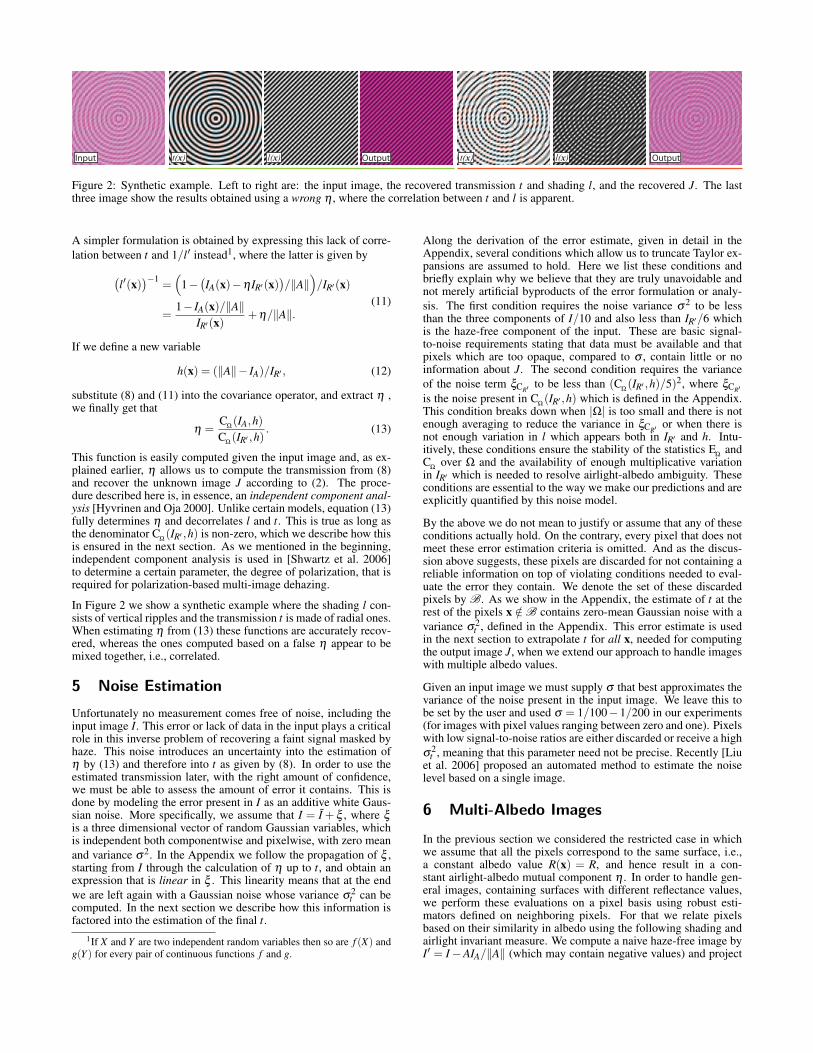
Figure 2: Synthetic example. Left to right are: the input image, the recovered transmission t and shading l, and the recovered J. The lastthree image show the results obtained using a wrong η , where the correlation between t and l is apparent.

A simpler formulation is obtained by expressing this lack of corre-lation between t and 1/l′ instead1, where the latter is given by

(l′(x)

)−1 =(

1− (IA(x)−ηIR′(x)

)/‖A‖

)/IR′(x)

=1− IA(x)/‖A‖

IR′(x)+η/‖A‖.

(11)

If we define a new variable

h(x) = (‖A‖− IA)/IR′ , (12)

substitute (8) and (11) into the covariance operator, and extract η ,we finally get that

η =CΩ(IA,h)CΩ(IR′ ,h)

. (13)

This function is easily computed given the input image and, as ex-plained earlier, η allows us to compute the transmission from (8)and recover the unknown image J according to (2). The proce-dure described here is, in essence, an independent component anal-ysis [Hyvrinen and Oja 2000]. Unlike certain models, equation (13)fully determines η and decorrelates l and t. This is true as long asthe denominator CΩ(IR′ ,h) is non-zero, which we describe how thisis ensured in the next section. As we mentioned in the beginning,independent component analysis is used in [Shwartz et al. 2006]to determine a certain parameter, the degree of polarization, that isrequired for polarization-based multi-image dehazing.

In Figure 2 we show a synthetic example where the shading l con-sists of vertical ripples and the transmission t is made of radial ones.When estimating η from (13) these functions are accurately recov-ered, whereas the ones computed based on a false η appear to bemixed together, i.e., correlated.

5 Noise Estimation

Unfortunately no measurement comes free of noise, including theinput image I. This error or lack of data in the input plays a criticalrole in this inverse problem of recovering a faint signal masked byhaze. This noise introduces an uncertainty into the estimation ofη by (13) and therefore into t as given by (8). In order to use theestimated transmission later, with the right amount of confidence,we must be able to assess the amount of error it contains. This isdone by modeling the error present in I as an additive white Gaus-sian noise. More specifically, we assume that I = I + ξ , where ξis a three dimensional vector of random Gaussian variables, whichis independent both componentwise and pixelwise, with zero meanand variance σ2. In the Appendix we follow the propagation of ξ ,starting from I through the calculation of η up to t, and obtain anexpression that is linear in ξ . This linearity means that at the endwe are left again with a Gaussian noise whose variance σ2

t can becomputed. In the next section we describe how this information isfactored into the estimation of the final t.

1If X and Y are two independent random variables then so are f (X) andg(Y ) for every pair of continuous functions f and g.

Along the derivation of the error estimate, given in detail in theAppendix, several conditions which allow us to truncate Taylor ex-pansions are assumed to hold. Here we list these conditions andbriefly explain why we believe that they are truly unavoidable andnot merely artificial byproducts of the error formulation or analy-sis. The first condition requires the noise variance σ2 to be lessthan the three components of I/10 and also less than IR′/6 whichis the haze-free component of the input. These are basic signal-to-noise requirements stating that data must be available and thatpixels which are too opaque, compared to σ , contain little or noinformation about J. The second condition requires the varianceof the noise term ξCR′ to be less than (CΩ(IR′ ,h)/5)2, where ξCR′is the noise present in CΩ(IR′ ,h) which is defined in the Appendix.This condition breaks down when |Ω| is too small and there is notenough averaging to reduce the variance in ξCR′ or when there isnot enough variation in l which appears both in IR′ and h. Intu-itively, these conditions ensure the stability of the statistics EΩ andCΩ over Ω and the availability of enough multiplicative variationin IR′ which is needed to resolve airlight-albedo ambiguity. Theseconditions are essential to the way we make our predictions and areexplicitly quantified by this noise model.

By the above we do not mean to justify or assume that any of theseconditions actually hold. On the contrary, every pixel that does notmeet these error estimation criteria is omitted. And as the discus-sion above suggests, these pixels are discarded for not containing areliable information on top of violating conditions needed to eval-uate the error they contain. We denote the set of these discardedpixels by B. As we show in the Appendix, the estimate of t at therest of the pixels x /∈B contains zero-mean Gaussian noise with avariance σ2

t , defined in the Appendix. This error estimate is usedin the next section to extrapolate t for all x, needed for computingthe output image J, when we extend our approach to handle imageswith multiple albedo values.

Given an input image we must supply σ that best approximates thevariance of the noise present in the input image. We leave this tobe set by the user and used σ = 1/100−1/200 in our experiments(for images with pixel values ranging between zero and one). Pixelswith low signal-to-noise ratios are either discarded or receive a highσ2

t , meaning that this parameter need not be precise. Recently [Liuet al. 2006] proposed an automated method to estimate the noiselevel based on a single image.

6 Multi-Albedo Images

In the previous section we considered the restricted case in whichwe assume that all the pixels correspond to the same surface, i.e.,a constant albedo value R(x) = R, and hence result in a con-stant airlight-albedo mutual component η . In order to handle gen-eral images, containing surfaces with different reflectance values,we perform these evaluations on a pixel basis using robust esti-mators defined on neighboring pixels. For that we relate pixelsbased on their similarity in albedo using the following shading andairlight invariant measure. We compute a naive haze-free image byI′ = I−AIA/‖A‖ (which may contain negative values) and project

t^

σt

σs

t

IA

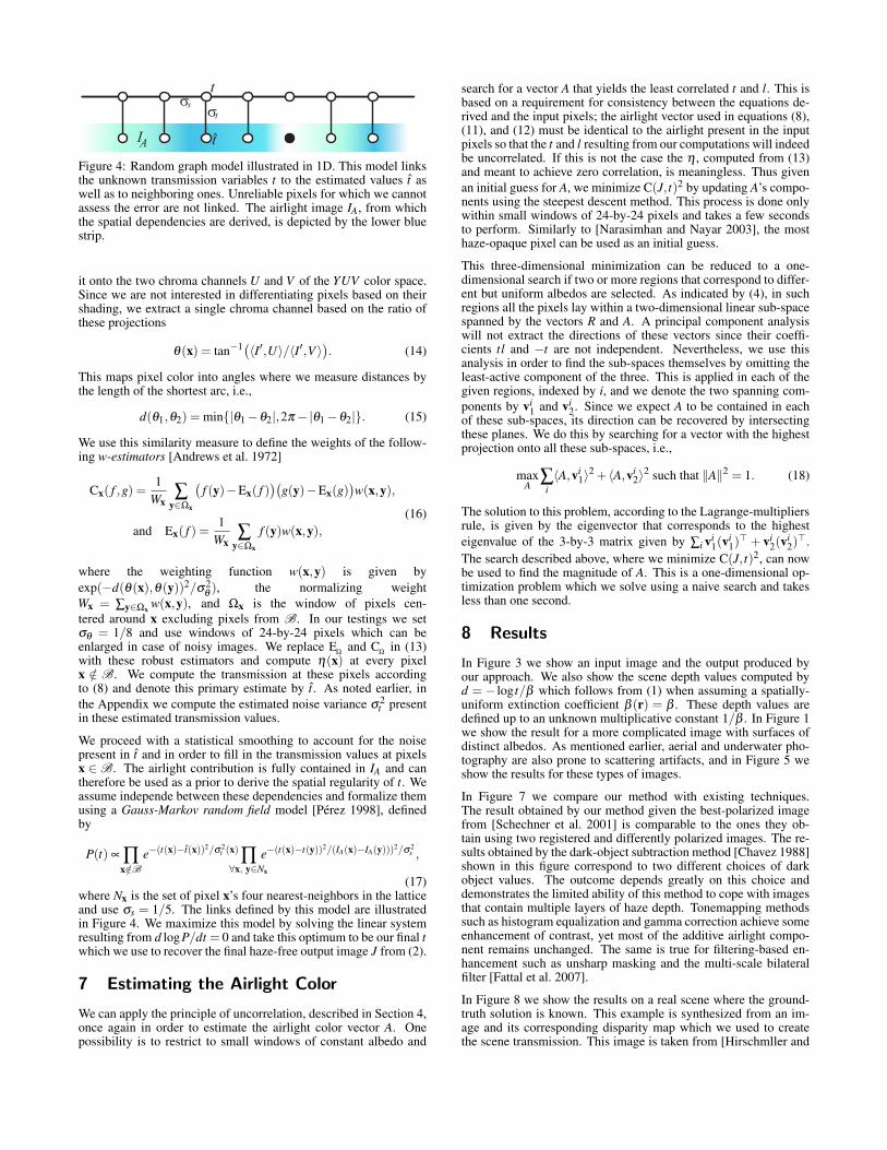
Figure 4: Random graph model illustrated in 1D. This model linksthe unknown transmission variables t to the estimated values t aswell as to neighboring ones. Unreliable pixels for which we cannotassess the error are not linked. The airlight image IA, from whichthe spatial dependencies are derived, is depicted by the lower bluestrip.

it onto the two chroma channels U and V of the YUV color space.Since we are not interested in differentiating pixels based on theirshading, we extract a single chroma channel based on the ratio ofthese projections

θ(x) = tan−1(〈I′,U〉/〈I′,V 〉). (14)

This maps pixel color into angles where we measure distances bythe length of the shortest arc, i.e.,

d(θ1,θ2) = min|θ1−θ2|,2π−|θ1−θ2|. (15)

We use this similarity measure to define the weights of the follow-ing w-estimators [Andrews et al. 1972]

Cx( f ,g) =1

Wx∑

y∈Ωx

(f (y)−Ex( f )

)(g(y)−Ex(g)

)w(x,y),

and Ex( f ) =1

Wx∑

y∈Ωx

f (y)w(x,y),(16)

where the weighting function w(x,y) is given byexp(−d(θ(x),θ(y))2/σ2

θ ), the normalizing weightWx = ∑y∈Ωx w(x,y), and Ωx is the window of pixels cen-tered around x excluding pixels from B. In our testings we setσθ = 1/8 and use windows of 24-by-24 pixels which can beenlarged in case of noisy images. We replace EΩ and CΩ in (13)with these robust estimators and compute η(x) at every pixelx /∈ B. We compute the transmission at these pixels accordingto (8) and denote this primary estimate by t. As noted earlier, inthe Appendix we compute the estimated noise variance σ2

t presentin these estimated transmission values.

We proceed with a statistical smoothing to account for the noisepresent in t and in order to fill in the transmission values at pixelsx ∈ B. The airlight contribution is fully contained in IA and cantherefore be used as a prior to derive the spatial regularity of t. Weassume independe between these dependencies and formalize themusing a Gauss-Markov random field model [Perez 1998], definedby

P(t) ∝ ∏x/∈B

e−(t(x)−t(x))2/σ 2t (x) ∏∀x, y∈Nx

e−(t(x)−t(y))2/(IA(x)−IA(y)))2/σ 2s ,

(17)where Nx is the set of pixel x’s four nearest-neighbors in the latticeand use σs = 1/5. The links defined by this model are illustratedin Figure 4. We maximize this model by solving the linear systemresulting from d logP/dt = 0 and take this optimum to be our final twhich we use to recover the final haze-free output image J from (2).

7 Estimating the Airlight Color

We can apply the principle of uncorrelation, described in Section 4,once again in order to estimate the airlight color vector A. Onepossibility is to restrict to small windows of constant albedo and

search for a vector A that yields the least correlated t and l. This isbased on a requirement for consistency between the equations de-rived and the input pixels; the airlight vector used in equations (8),(11), and (12) must be identical to the airlight present in the inputpixels so that the t and l resulting from our computations will indeedbe uncorrelated. If this is not the case the η , computed from (13)and meant to achieve zero correlation, is meaningless. Thus givenan initial guess for A, we minimize C(J, t)2 by updating A’s compo-nents using the steepest descent method. This process is done onlywithin small windows of 24-by-24 pixels and takes a few secondsto perform. Similarly to [Narasimhan and Nayar 2003], the mosthaze-opaque pixel can be used as an initial guess.

This three-dimensional minimization can be reduced to a one-dimensional search if two or more regions that correspond to differ-ent but uniform albedos are selected. As indicated by (4), in suchregions all the pixels lay within a two-dimensional linear sub-spacespanned by the vectors R and A. A principal component analysiswill not extract the directions of these vectors since their coeffi-cients tl and −t are not independent. Nevertheless, we use thisanalysis in order to find the sub-spaces themselves by omitting theleast-active component of the three. This is applied in each of thegiven regions, indexed by i, and we denote the two spanning com-ponents by vi

1 and vi2. Since we expect A to be contained in each

of these sub-spaces, its direction can be recovered by intersectingthese planes. We do this by searching for a vector with the highestprojection onto all these sub-spaces, i.e.,

maxA

∑i〈A,vi

1〉2 + 〈A,vi2〉2 such that ‖A‖2 = 1. (18)

The solution to this problem, according to the Lagrange-multipliersrule, is given by the eigenvector that corresponds to the highesteigenvalue of the 3-by-3 matrix given by ∑i vi

1(vi1)> + vi

2(vi2)>.

The search described above, where we minimize C(J, t)2, can nowbe used to find the magnitude of A. This is a one-dimensional op-timization problem which we solve using a naive search and takesless than one second.

8 Results

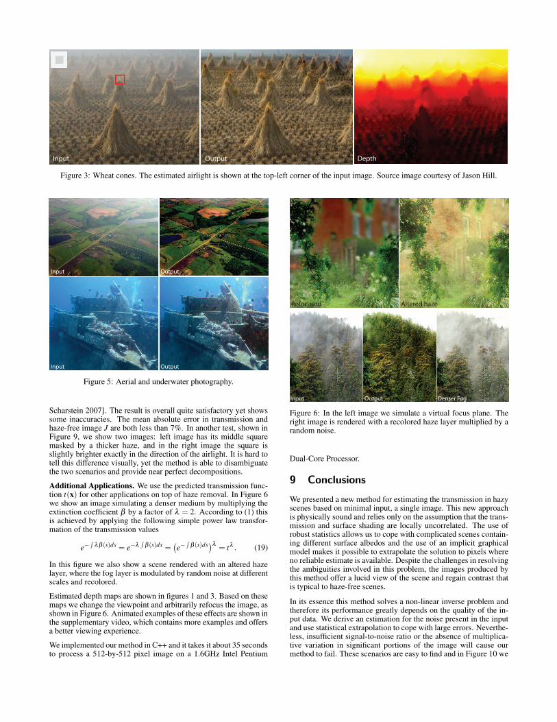
In Figure 3 we show an input image and the output produced byour approach. We also show the scene depth values computed byd = − log t/β which follows from (1) when assuming a spatially-uniform extinction coefficient β (r) = β . These depth values aredefined up to an unknown multiplicative constant 1/β . In Figure 1we show the result for a more complicated image with surfaces ofdistinct albedos. As mentioned earlier, aerial and underwater pho-tography are also prone to scattering artifacts, and in Figure 5 weshow the results for these types of images.

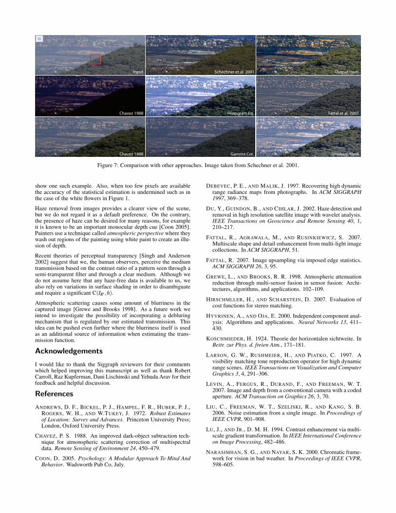
In Figure 7 we compare our method with existing techniques.The result obtained by our method given the best-polarized imagefrom [Schechner et al. 2001] is comparable to the ones they ob-tain using two registered and differently polarized images. The re-sults obtained by the dark-object subtraction method [Chavez 1988]shown in this figure correspond to two different choices of darkobject values. The outcome depends greatly on this choice anddemonstrates the limited ability of this method to cope with imagesthat contain multiple layers of haze depth. Tonemapping methodssuch as histogram equalization and gamma correction achieve someenhancement of contrast, yet most of the additive airlight compo-nent remains unchanged. The same is true for filtering-based en-hancement such as unsharp masking and the multi-scale bilateralfilter [Fattal et al. 2007].

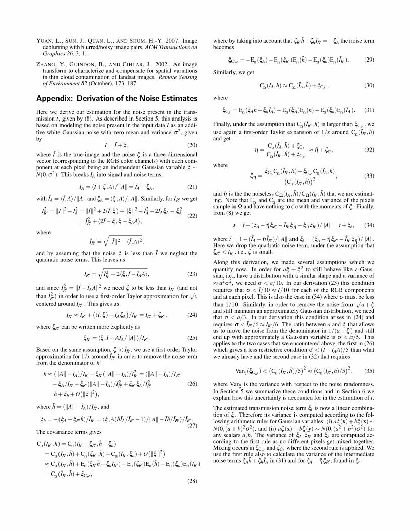
In Figure 8 we show the results on a real scene where the ground-truth solution is known. This example is synthesized from an im-age and its corresponding disparity map which we used to createthe scene transmission. This image is taken from [Hirschmller and

Input Output Depth

Figure 3: Wheat cones. The estimated airlight is shown at the top-left corner of the input image. Source image courtesy of Jason Hill.

Input

Input

Output

Output

Figure 5: Aerial and underwater photography.

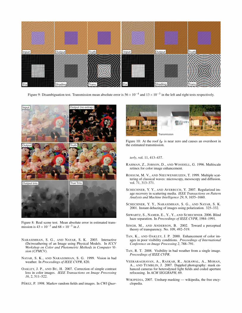
Scharstein 2007]. The result is overall quite satisfactory yet showssome inaccuracies. The mean absolute error in transmission andhaze-free image J are both less than 7%. In another test, shown inFigure 9, we show two images: left image has its middle squaremasked by a thicker haze, and in the right image the square isslightly brighter exactly in the direction of the airlight. It is hard totell this difference visually, yet the method is able to disambiguatethe two scenarios and provide near perfect decompositions.

Additional Applications. We use the predicted transmission func-tion t(x) for other applications on top of haze removal. In Figure 6we show an image simulating a denser medium by multiplying theextinction coefficient β by a factor of λ = 2. According to (1) thisis achieved by applying the following simple power law transfor-mation of the transmission values

e−∫

λβ (s)ds = e−λ∫

β (s)ds =(e−

∫β (s)ds)λ = tλ . (19)

In this figure we also show a scene rendered with an altered hazelayer, where the fog layer is modulated by random noise at differentscales and recolored.

Estimated depth maps are shown in figures 1 and 3. Based on thesemaps we change the viewpoint and arbitrarily refocus the image, asshown in Figure 6. Animated examples of these effects are shown inthe supplementary video, which contains more examples and offersa better viewing experience.

We implemented our method in C++ and it takes it about 35 secondsto process a 512-by-512 pixel image on a 1.6GHz Intel Pentium

Altered hazeRefocused

OutputInput Denser Fog

Figure 6: In the left image we simulate a virtual focus plane. Theright image is rendered with a recolored haze layer multiplied by arandom noise.

Dual-Core Processor.

9 Conclusions

We presented a new method for estimating the transmission in hazyscenes based on minimal input, a single image. This new approachis physically sound and relies only on the assumption that the trans-mission and surface shading are locally uncorrelated. The use ofrobust statistics allows us to cope with complicated scenes contain-ing different surface albedos and the use of an implicit graphicalmodel makes it possible to extrapolate the solution to pixels whereno reliable estimate is available. Despite the challenges in resolvingthe ambiguities involved in this problem, the images produced bythis method offer a lucid view of the scene and regain contrast thatis typical to haze-free scenes.

In its essence this method solves a non-linear inverse problem andtherefore its performance greatly depends on the quality of the in-put data. We derive an estimation for the noise present in the inputand use statistical extrapolation to cope with large errors. Neverthe-less, insufficient signal-to-noise ratio or the absence of multiplica-tive variation in significant portions of the image will cause ourmethod to fail. These scenarios are easy to find and in Figure 10 we

Input Schechner et al. 2001 Output (our)

Chavez 1988 Histogram Eq.

Gamma Cor.

Fattal et al. 2007

Gamma Cor. Unsharp MaskChavez 1988

Figure 7: Comparison with other approaches. Image taken from Schechner et al. 2001.

show one such example. Also, when too few pixels are availablethe accuracy of the statistical estimation is undermined such as inthe case of the white flowers in Figure 1.

Haze removal from images provides a clearer view of the scene,but we do not regard it as a default preference. On the contrary,the presence of haze can be desired for many reasons, for exampleit is known to be an important monocular depth cue [Coon 2005].Painters use a technique called atmospheric perspective where theywash out regions of the painting using white paint to create an illu-sion of depth.

Recent theories of perceptual transparency [Singh and Anderson2002] suggest that we, the human observers, perceive the mediumtransmission based on the contrast ratio of a pattern seen through asemi-transparent filter and through a clear medium. Although wedo not assume here that any haze-free data is available to us, wealso rely on variations in surface shading in order to disambiguateand require a significant C(IR′ ,h).

Atmospheric scattering causes some amount of blurriness in thecaptured image [Grewe and Brooks 1998]. As a future work weintend to investigate the possibility of incorporating a debluringmechanism that is regulated by our estimated transmission. Thisidea can be pushed even further where the blurriness itself is usedas an additional source of information when estimating the trans-mission function.

Acknowledgements

I would like to thank the Siggraph reviewers for their commentswhich helped improving this manuscript as well as thank RobertCarroll, Raz Kupferman, Dani Lischinski and Yehuda Arav for theirfeedback and helpful discussion.

References

ANDREWS, D. F., BICKEL, P. J., HAMPEL, F. R., HUBER, P. J.,ROGERS, W. H., AND W.TUKEY, J. 1972. Robust Estimatesof Location: Survey and Advances. Princeton University Press;London, Oxford University Press.

CHAVEZ, P. S. 1988. An improved dark-object subtraction tech-nique for atmonspheric scattering correction of multispectraldata. Remote Sensing of Environment 24, 450–479.

COON, D. 2005. Psychology: A Modular Approach To Mind AndBehavior. Wadsworth Pub Co, July.

DEBEVEC, P. E., AND MALIK, J. 1997. Recovering high dynamicrange radiance maps from photographs. In ACM SIGGRAPH1997, 369–378.

DU, Y., GUINDON, B., AND CIHLAR, J. 2002. Haze detection andremoval in high resolution satellite image with wavelet analysis.IEEE Transactions on Geoscience and Remote Sensing 40, 1,210–217.

FATTAL, R., AGRAWALA, M., AND RUSINKIEWICZ, S. 2007.Multiscale shape and detail enhancement from multi-light imagecollections. In ACM SIGGRAPH, 51.

FATTAL, R. 2007. Image upsampling via imposed edge statistics.ACM SIGGRAPH 26, 3, 95.

GREWE, L., AND BROOKS, R. R. 1998. Atmospheric attenuationreduction through multi-sensor fusion in sensor fusion: Archi-tectures, algorithms, and applications. 102–109.

HIRSCHMLLER, H., AND SCHARSTEIN, D. 2007. Evaluation ofcost functions for stereo matching.

HYVRINEN, A., AND OJA, E. 2000. Independent component anal-ysis: Algorithms and applications. Neural Networks 13, 411–430.

KOSCHMIEDER, H. 1924. Theorie der horizontalen sichtweite. InBeitr. zur Phys. d. freien Atm., 171–181.

LARSON, G. W., RUSHMEIER, H., AND PIATKO, C. 1997. Avisibility matching tone reproduction operator for high dynamicrange scenes. IEEE Transactions on Visualization and ComputerGraphics 3, 4, 291–306.

LEVIN, A., FERGUS, R., DURAND, F., AND FREEMAN, W. T.2007. Image and depth from a conventional camera with a codedaperture. ACM Transaction on Graphics 26, 3, 70.

LIU, C., FREEMAN, W. T., SZELISKI, R., AND KANG, S. B.2006. Noise estimation from a single image. In Proceedings ofIEEE CVPR, 901–908.

LU, J., AND JR., D. M. H. 1994. Contrast enhancement via multi-scale gradient transformation. In IEEE International Conferenceon Image Processing, 482–486.

NARASIMHAN, S. G., AND NAYAR, S. K. 2000. Chromatic frame-work for vision in bad weather. In Proceedings of IEEE CVPR,598–605.

Input Output Truth

Eta Shading Trans.

Input Output Truth

Eta Shading Trans.

Figure 9: Disambiguation test. Transmission mean absolute error is 56×10−4 and 13×10−3 in the left and right tests respectively.

Input Output (no extrap.)

Output Truth

True Trns.Output trns.

Figure 8: Real scene test. Mean absolute error in estimated trans-mission is 43×10−3 and 68×10−3 in J.

NARASIMHAN, S. G., AND NAYAR, S. K. 2003. Interactive(De)weathering of an Image using Physical Models. In ICCVWorkshop on Color and Photometric Methods in Computer Vi-sion (CPMCV).

NAYAR, S. K., AND NARASIMHAN, S. G. 1999. Vision in badweather. In Proceedings of IEEE CVPR, 820.

OAKLEY, J. P., AND BU, H. 2007. Correction of simple contrastloss in color images. IEEE Transactions on Image Processing16, 2, 511–522.

PEREZ, P. 1998. Markov random fields and images. In CWI Quar-

Input Transmission Output

Figure 10: At the roof IR′ is near zero and causes an overshoot inthe estimated transmission.

terly, vol. 11, 413–437.

RAHMAN, Z., JOBSON, D., AND WOODELL, G. 1996. Multiscaleretinex for color image enhancement.

ROSSUM, M. V., AND NIEUWENHUIZEN, T. 1999. Multiple scat-tering of classical waves: microscopy, mesoscopy and diffusion.vol. 71, 313–371.

SCHECHNER, Y. Y., AND AVERBUCH, Y. 2007. Regularized im-age recovery in scattering media. IEEE Transactions on PatternAnalysis and Machine Intelligence 29, 9, 1655–1660.

SCHECHNER, Y. Y., NARASIMHAN, S. G., AND NAYAR, S. K.2001. Instant dehazing of images using polarization. 325–332.

SHWARTZ, S., NAMER, E., Y., Y., AND SCHECHNER. 2006. Blindhaze separation. In Proceedings of IEEE CVPR, 1984–1991.

SINGH, M., AND ANDERSON, B. 2002. Toward a perceptualtheory of transparency. No. 109, 492–519.

TAN, K., AND OAKLEY, J. P. 2000. Enhancement of color im-ages in poor visibility conditions. Proceedings of InternationalConference on Image Processing 2, 788–791.

TAN, R. T. 2008. Visibility in bad weather from a single image.Proceedings of IEEE CVPR.

VEERARAGHAVAN, A., RASKAR, R., AGRAWAL, A., MOHAN,A., AND TUMBLIN, J. 2007. Dappled photography: mask en-hanced cameras for heterodyned light fields and coded aperturerefocusing. In ACM SIGGRAPH, 69.

WIKIPEDIA, 2007. Unsharp masking — wikipedia, the free ency-clopedia.

YUAN, L., SUN, J., QUAN, L., AND SHUM, H.-Y. 2007. Imagedeblurring with blurred/noisy image pairs. ACM Transactions onGraphics 26, 3, 1.

ZHANG, Y., GUINDON, B., AND CIHLAR, J. 2002. An imagetransform to characterize and compensate for spatial variationsin thin cloud contamination of landsat images. Remote Sensingof Environment 82 (October), 173–187.

Appendix: Derivation of the Noise Estimates

Here we derive our estimation for the noise present in the trans-mission t, given by (8). As described in Section 5, this analysis isbased on modeling the noise present in the input data I as an addi-tive white Gaussian noise with zero mean and variance σ2, givenby

I = I +ξ , (20)

where I is the true image and the noise ξ is a three-dimensionalvector (corresponding to the RGB color channels) with each com-ponent at each pixel being an independent Gaussian variable ξ ∼N(0,σ2). This breaks IA into signal and noise terms,

IA = 〈I +ξ ,A〉/‖A‖= IA +ξA, (21)

with IA = 〈I,A〉/‖A‖ and ξA = 〈ξ ,A〉/‖A‖. Similarly, for IR′ we get

I2R′ = ‖I‖2− I2

A = ‖I‖2 +2〈I,ξ 〉+‖ξ‖2− I2A−2IAξA−ξ 2

A

= I2R′ + 〈2I−ξ ,ξ −ξAA〉,

(22)

whereIR′ =

√‖I‖2−〈I,A〉2,

and by assuming that the noise ξ is less than I we neglect thequadratic noise terms. This leaves us

IR′ =√

I2R′ +2〈ξ , I− IAA〉, (23)

and since I2R′ = ‖I− IAA‖2 we need ξ to be less than IR′ (and not

than I2R′ ) in order to use a first-order Taylor approximation for

√x

centered around IR′ . This gives us

IR′ ≈ IR′ +(〈I,ξ 〉− IAξA

)/IR′ = IR′ +ξR′ , (24)

where ξR′ can be written more explicitly as

ξR′ = 〈ξ , I−AIA/‖A‖〉/IR′ . (25)

Based on the same assumption, ξ < IR′ , we use a first-order Taylorapproximation for 1/x around IR′ in order to remove the noise termfrom the denominator of h

h≈ (‖A‖− IA)/IR′ −ξR′(‖A‖− IA)/I2R′ = (‖A‖− IA)/IR′

−ξA/IR′ −ξR′(‖A‖− IA)/I2R′ +ξR′ξA/I2

R′

= h+ξh +O(‖ξ‖2),

(26)

where h = (‖A‖− IA)/IR′ , and

ξh =−(ξA +ξR′ h)/IR′ = 〈ξ ,A(hIA/IR′ −1)/‖A‖− Ih/IR′〉/IR′ .(27)

The covariance terms gives

CΩ(IR′ ,h) = CΩ(IR′ +ξR′ , h+ξh)

= CΩ(IR′ , h)+CΩ(ξR′ , h)+CΩ(IR′ ,ξh)+O(‖ξ‖2)

≈ CΩ(IR′ , h)+EΩ(ξR′ h+ξh IR′)−EΩ(ξR′)EΩ(h)−EΩ(ξh)EΩ(IR′)

= CΩ(IR′ , h)+ξCR′ ,(28)

where by taking into account that ξR′ h+ξh IR′ =−ξA the noise termbecomes

ξCR′ =−EΩ(ξA)−EΩ(ξR′)EΩ(h)−EΩ(ξh)EΩ(IR′). (29)

Similarly, we get

CΩ(IA,h)≈ CΩ(IA, h)+ξCA , (30)

where

ξCA = EΩ(ξAh+ξh IA)−EΩ(ξA)EΩ(h)−EΩ(ξh)EΩ(IA). (31)

Finally, under the assumption that CΩ(IR′ , h) is larger than ξCR′ , weuse again a first-order Taylor expansion of 1/x around CΩ(IR′ , h)and get

η =CΩ(IA, h)+ξCA

CΩ(IR′ , h)+ξCR′≈ η +ξη , (32)

where

ξη =ξCA CΩ(IR′ , h)−ξCR′ CΩ(IA, h)

(CΩ(IR′ , h)

)2 , (33)

and η is the the noiseless CΩ(IA, h)/CΩ(IR′ , h) that we are estimat-ing. Note that EΩ and CΩ are the mean and variance of the pixelssample in Ω and have nothing to do with the moments of ξ . Finally,from (8) we get

t = t +(ξA− ηξR′ − IR′ξη −ξη ξR′)/‖A‖= t +ξt , (34)

where t = 1− (IA− η IR′)/‖A‖ and ξt = (ξA− ηξR′ − IR′ξη )/‖A‖.Here we drop the quadratic noise term, under the assumption thatξR′ < IR′ , i.e., ξ is small.

Along this derivation, we made several assumptions which wequantify now. In order for aξ + ξ 2 to still behave like a Gaus-sian, i.e., have a distribution with a similar shape and a variance of≈ a2σ2, we need σ < a/10. In our derivation (23) this conditionrequires that σ < I/10 ≈ I/10 for each of the RGB componentsand at each pixel. This is also the case in (34) where σ must be lessthan 1/10. Similarly, in order to remove the noise from

√a+ξ

and still maintain an approximately Gaussian distribution, we needthat σ < a/3. In our derivation this condition arises in (24) andrequires σ < IR′/6 ≈ IR′/6. The ratio between a and ξ that allowsus to move the noise from the denominator in 1/(a + ξ ) and stillend up with approximately a Gaussian variable is σ < a/5. Thisapplies to the two cases that we encountered above, the first in (26)which gives a less restrictive condition σ < (I− IAA)/5 than whatwe already have and the second case in (32) that requires

Varξ (ξCR′ ) <(CΩ(IR′ , h)/5

)2 ≈ (CΩ(IR′ ,h)/5

)2, (35)

where Varξ is the variance with respect to the noise randomness.In Section 5 we summarize these conditions and in Section 6 weexplain how this uncertainly is accounted for in the estimation of t.

The estimated transmission noise term ξt is now a linear combina-tion of ξ . Therefore its variance is computed according to the fol-lowing arithmetic rules for Gaussian variables: (i) aξ (x)+bξ (x)∼N(0,(a + b)2σ2), and (ii) aξ (x)+ bξ (y) ∼ N(0,(a2 + b2)σ2) forany scalars a,b. The variance of ξA,ξR′ and ξh are computed ac-cording to the first rule as no different pixels get mixed together.Mixing occurs in ξCR′ and ξCh where the second rule is applied. Weuse the first rule also to calculate the variance of the intermediatenoise terms ξAh+ξh IA in (31) and for ξA− ηξR′ , found in ξt .