Single machine earliness–tardiness scheduling with resource-dependent release dates

Discrete Optimization

Single machine earliness–tardiness scheduling withresource-dependent release dates

Jos�ee A. Ventura a,*, Daecheol Kim b, Frederic Garriga c

a Harold and Inge Marcus Department of Industrial and Manufacturing Engineering, 356 Leonhard Building,

Pennsylvania State University, University Park, PA 16802, USAb AspenTech, 8th Floor, 63 Building, 60 Yoido-dong, Youngdeungpo-ku, Seoul, 150-763, South Korea

c Departament d’Organitzaci�oo d’Empreses, Escola T�eecnica Superior d’Enginyeria Industrial, Universitat Polit�eecnica de Catalunya,Col�oon, 11, 08222-Terrassa (Barcelona), Spain

Received 26 August 1999; accepted 15 August 2001

Abstract

This paper deals with the single machine earliness and tardiness scheduling problem with a common due date and

resource-dependent release dates. It is assumed that the cost of resource consumption of a job is a non-increasing linear

function of the job release date, and this function is common for all jobs. The objective is to find a schedule and job

release dates that minimize the total resource consumption, and earliness and tardiness penalties. It is shown that the

problem is NP-hard in the ordinary sense even if the due date is unrestricted (the number of jobs that can be scheduled

before the due date is unrestricted). An exact dynamic programming (DP) algorithm for small and medium size

problems is developed. A heuristic algorithm for large-scale problems is also proposed and the results of a computa-

tional comparison between heuristic and optimal solutions are discussed.

� 2002 Elsevier Science B.V. All rights reserved.

Keywords: Scheduling theory; Dynamic programming; Heuristics; Computational analysis

1. Introduction

In classical scheduling models, job release times are often ignored and assumed to be zero. Even in thecase where they are considered, they are provided as constants known prior to scheduling [4,18]. In manymanufacturing environments, however, a job needs to be preprocessed before it undergoes process-ing [10,11,15,16]. This preprocessing time can be considered as job release time, and it depends on the

European Journal of Operational Research 142 (2002) 52–69

www.elsevier.com/locate/dsw

*Corresponding author. Tel.: +1-814-865-3841; fax: +1-814-865-4745.

E-mail address: [email protected] (J.A. Ventura).

0377-2217/02/$ - see front matter � 2002 Elsevier Science B.V. All rights reserved.

PII: S0377 -2217 (01 )00292 -2

mail to: [email protected]

resource consumed for the preprocessing treatment. Hence, job release times are variables. A practicalexample of such a scheduling problem can be found in steel production. Ingots must be preheated by gasin soaking pits to the required temperature, before they can be hot-rolled by a blooming mill [12,17]. Thepreheating time of an ingot is a non-increasing function of the amount of gas consumed. Thus, thepreheating time of an ingot may be treated as the release time at which the ingot is available for the job ofingot rolling.Several single machine scheduling models have emerged to control the total resource consumption as

well as other quantities such as schedule length, sum of job completion times, and mean tardiness of jobs.Janiak [9] considered the problem of minimizing the schedule length subject to a constraint on the totalresource consumption with resource-dependent release times on a single machine. In his scheduling model,the release time of each job is assumed to be a positive linear decreasing function of the resource con-sumed for that job. Li [15] analyzed the problem of minimizing the total resource consumption with acontrol on the job completion times. He compared several scheduling methods for the case where theresource consumption function is common to all jobs and the case where the resource consumption isproportional to the job processing time. Li [16] considered the problem of minimizing the total resourceconsumption with a constraint on the sum of job completion times. He showed that the single and parallelmachine problems can be efficiently solved if the resource consumption function is linear. Vasilev andFoote [20] studied the problem of minimizing the total resource consumption with constraints on themakespan and the total completion time. An extension of the results found by Li [16] to the case wherethe resource consumption function is convex and decreasing was presented. Recently, Li et al. [17]considered the minimization of the total resource consumption and the total job tardiness on a singlemachine with a non-increasing convex resource consumption function. Although the mean tardinesscriterion recognizes the loss of customers when jobs are finished late, it ignores the cost of early com-pletion of jobs.Penalizing earliness and tardiness (E–T) has been an important objective in recent scheduling research

due to the increasing emphasis on commitment to due dates [2,3,6,14]. An important special case in thefamily of E–T problems involves minimizing the sum of absolute deviations of job completion times from acommon due date [7,13,21–23]. A common due date model can represent a situation where several itemsconstitute a single customer’s order, or it might reflect an assembly environment in which the componentsshould all be ready at the same time to avoid staging delays.Kanet [13] presented a simple polynomial time algorithm to minimize the mean unweighted absolute

deviation of job completion times from a given common due date. In his study, he assumed that the duedate is late enough not to act as a constraint on the scheduling decision. Sundararaghavan and Ahmed [19]noticed that the optimal schedule generated by Kanet’s algorithm could violate the zero-ready-time as-sumption if the given due date is restrictively small. This notion gives rise to the restricted and unrestrictedversions of the mean absolute deviation (MAD) problem. Hall and Posner [7] and Bagchi et al. [1] discussedoptimality conditions for the MAD problem. While the unrestricted version of the MAD problem canbe solved in polynomial time, the restricted version was demonstrated to be NP-hard in the ordinary sense[8].The problem considered in this paper is to find a non-preemptive schedule that minimizes the total cost

caused by E–T and the amount of resource consumption on a single machine. The precise problemstatement is as follows. Let N ¼ f1; 2; . . . ; ng be a set of n independent jobs with known integer processingtimes, p1; . . . ; pn, and d a known integer common due date which is assumed to be greater than or equal tothe sum of all processing times. Denote by e and t the non-negative penalties per unit time charged for earlyand tardy job completion about the common due date, respectively. Job i is available after its release time riwhich is related to the amount of resource consumed. It is assumed that the resource consumption of job i isa non-increasing linear function with respect to its release time, and this resource consumption functionf ðrÞ is common for all jobs, i.e.,

J.A. Ventura et al. / European Journal of Operational Research 142 (2002) 52–69 53

f ðrÞ ¼ a� br if r6 d 0;0 if r > d 0;

�

where a and b are known positive parameters and d 0 ¼ a=b.Since the resource consumption function f ðriÞ is non-increasing, there exists an optimal solution such

that ri is set equal to the start time si of job i. Then ci, the completion time of job i, can be expressed asci ¼ si þ pi. Problem P can be formulated as follows:

ðPÞ minr2P

zðrÞ ¼Xni¼1

f ðriÞ½ þ emaxf0; d � cig þ tmaxf0; ci � dg�;

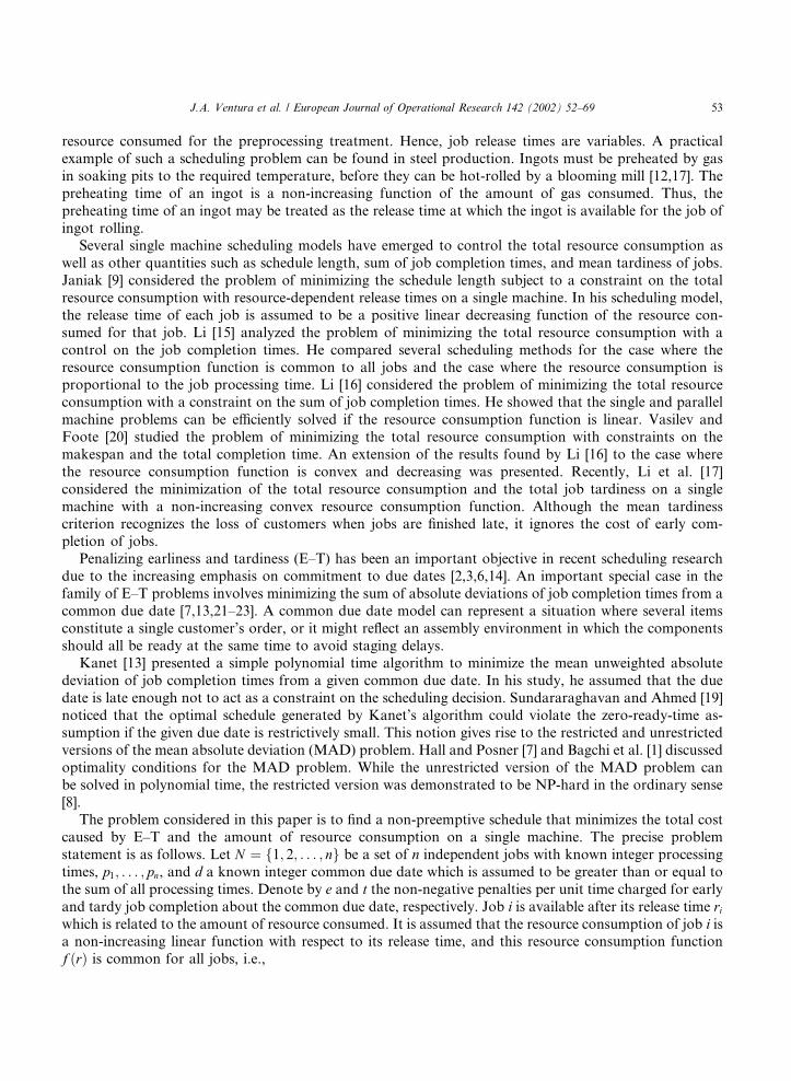
where r is a feasible schedule and P is the set of all feasible schedules.Consider the function gðrÞ ¼ f ðrÞ þ emaxf0; d � ðr þ pÞg þ tmaxf0; ðr þ pÞ � dg, as similarly defined in

[17]. Since f ðrÞ, maxf0; d � ðr þ pÞg, and maxf0; ðr þ pÞ � dg are piecewise linear and convex functions,gðrÞ is also piecewise linear and convex. Define q ¼ minfr0 P 0 jgðr0Þ6 gðrÞ for all rP 0g. That is, q is thefirst point at which gðrÞ attains its minimum. The function gðrÞ has three different shapes in terms of q andthe relative position of d 0 with respect to d, as shown in Fig. 1. If d 0

6 d, q is obtained at d (see Fig. 1(a)). Ifd 0 > d and b6 t, q is also obtained at d (see Fig. 1(b)). If d 0 > d and b > t; q is obtained at d 0 (see Fig. 1(c)).Throughout the paper, let j j denote set cardinality, ½ � job position in a schedule, and A½ � job position inset A.The rest of this paper is organized into four sections. Section 2 presents some dominance properties and

shows that the problem is NP-hard in the ordinary sense even if the common due date is unrestricted. Anexact dynamic programming (DP) procedure for small and medium size problems, and a heuristic algo-rithm for large-scale problems are developed in Section 3. This paper is concluded with a computationalstudy to assess the performance of the proposed heuristic algorithm in Section 4, and a summary of thecontributions of this study in Section 5.

2. Dominance properties

The dominance properties presented in this section are the basis for the proposed heuristic and DPalgorithms. The following two properties state that there exists an optimal schedule with no idle timebetween consecutive jobs and a job completing at time d or d 0.

Property 1. There exists an optimal solution for problem P with no idle time between any two consecutive jobs.

Proof. Similar to the proof of Theorem 1 in [17]. �

Fig. 1. Three different shapes of gðrÞ.

54 J.A. Ventura et al. / European Journal of Operational Research 142 (2002) 52–69

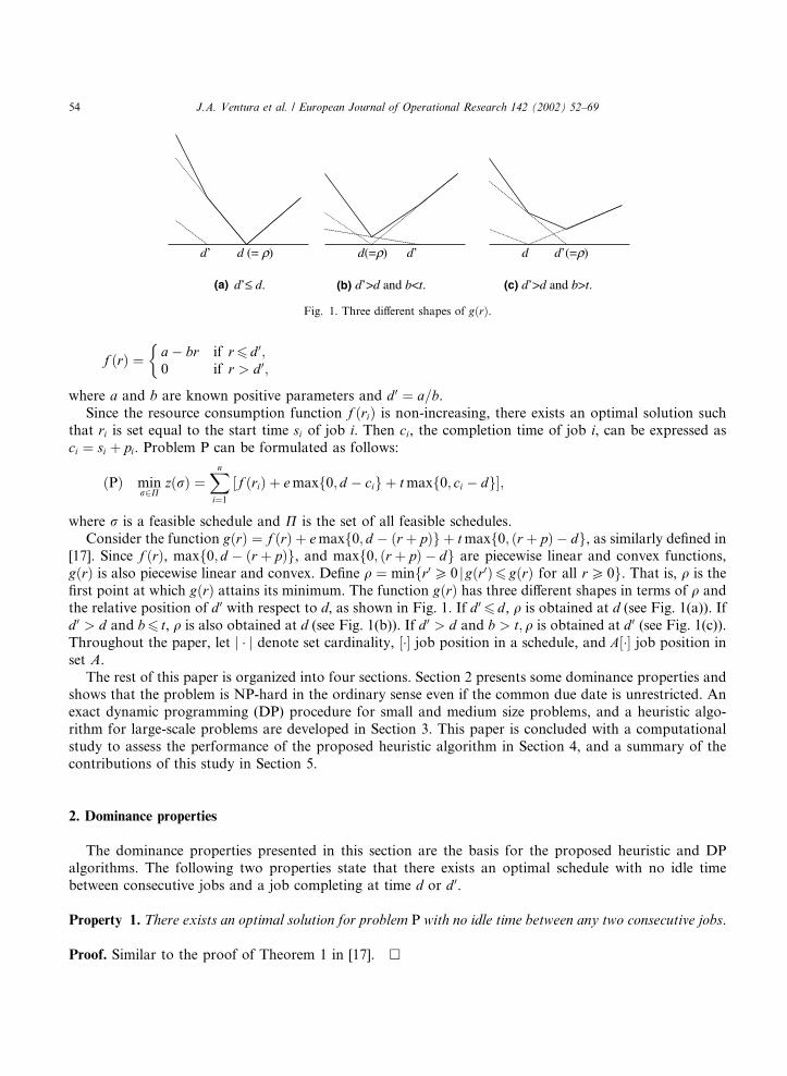
Property 2. There exists an optimal schedule for problem P such that at least one job starts or completes attime d or d 0.

Proof. Let r be an arbitrary schedule that does not satisfy Property 2. Assume that the ith job in schedule rstarts before and completes after d, and the jth job starts before and completes after d 0, as shown in Fig. 2.Let d1; d2; d3, and d4 be defined as in Fig. 2.By shifting schedule r to the left so that c½i� ¼ d if d26 d4, and c½j� ¼ d 0 if d2 > d4, the net change in total

cost becomes Dz0 ¼ d0½ði� 1Þe� ðn� iþ 1Þt þ jb�, where d0 ¼ minfd2; d4g. Similarly, shifting schedule r tothe right such that s½j� ¼ d 0 if d36 d1, and s½i� ¼ d if d3 > d1 causes the following net change in total cost,Dz00 ¼ �d00fði� 1Þe� ðn� iþ 1Þt þ jbg, where d00 ¼ minfd1; d3g. It is obvious that Dz0 6 0 if ði� 1Þe6ðn� iþ 1Þt � jb, and Dz00 6 0 if ði� 1ÞeP ðn� iþ 1Þt � jb.Therefore, for any schedule r that does not satisfy Property 2, an appropriate left or right shift of the

schedule always results in a new schedule which is not worse and that satisfies the dominance property. Thisimplies that there exists an optimal schedule in which at least one job starts or completes at time d or d 0.This completes the proof. �

Define E0 ¼ fi 2 N jci 6 qg and T 0 ¼ fi 2 N j si P qg. The following property states that there exists anoptimal weakly V-shaped schedule [8] for problem P.

Property 3. There exists an optimal schedule for problem P such that (i) the jobs in E0are arranged in LPTorder, (ii) the jobs in T 0 are arranged in SPT order, and (iii) if there is a job j with sj < q < cj and job j isneither the first nor the last job in the schedule, then pj 6 maxfpi; pkg, where jobs i and k are the jobs scheduledimmediately before and after job j, respectively.

Proof. Similar to the proof of Theorem 3 in [17]. �

The following three properties establish the cardinality of set E0 for any optimal schedule with a jobcompleting at time d or d 0.

Property 4. Given that d 06 d, if there exists an optimal schedule for problem P in which the kth and mth

jobs in sequence are such that s½k� < d 06 c½k� and c½m� ¼ d, then the number of jobs in E0 can be determined as

follows:

Fig. 2. Arbitrary schedules which do not satisfy Property 2.


jE0j ¼dðnt � kbÞ=ðeþ tÞe if ðnt � kbÞ=ðeþ tÞ is not integer;ðnt � kbÞ=ðeþ tÞ or ðnt � kbÞ=ðeþ tÞ þ 1 if ðnt � kbÞ=ðeþ tÞ is integer:

�

Proof. From Property 2 we know that there exists an optimal schedule in which one job completes at d or d 0.Let us assume that there is an optimal schedule r� in which d 0

6 d; s½k� < d 06 c½k�, and c½m� ¼ d. Since

schedule r� is optimal, the total penalty of a new schedule r0 which results from a right (or left) shift of theschedule should be greater than or equal to zðr�Þ.The right shift of schedule r� by D, where D > 0, causes an increase in the objective function of at least

Dðn� mþ 1Þt and a decrease of no more than Dfðm� 1Þeþ kbg. Therefore, the net change in total costbecomes Dfðn� mþ 1Þt � ðm� 1Þe� kbgP 0, or equivalently m6 ðnt � kbÞ=ðeþ tÞ þ 1.The left shift of schedule r� by D, where D > 0, causes an increase in the objective function of at least

Dðmeþ kbÞ and a decrease of no more than Dðn� mÞt. Therefore, the change in objective function value isD½meþ kb� ðn� mÞt�P 0, or equivalently mP ðnt � kbÞ=ðeþ tÞ.From the results of both cases, we know that ðnt � kbÞ=ðeþ tÞ6m6 ðnt � kbÞ=ðeþ tÞ þ 1. If ðnt � kbÞ=

ðeþ tÞ is integer, jE0j is either ðnt � kbÞ=ðeþ tÞ or ðnt � kbÞ=ðeþ tÞ þ 1. If ðnt � kbÞ=ðeþ tÞ is not integer,jE0j ¼ dðnt � kbÞ=ðeþ tÞe since jE0j should be an integer greater than or equal to ðnt � kbÞ=ðeþ tÞ and lessthan or equal to 1þ ðnt � kbÞ=ðeþ tÞ. This completes the proof. �

Property 5. Given that d 0 > d and b6 t, if there exists an optimal schedule for problem P in which the mth andðmþ kÞth jobs in sequence are such that c½m� ¼ d and s½mþk� < d 0

6 c½mþk�, then the number of jobs in E0 is equalto dðnt � kbÞ=ðeþ t þ bÞe.

Proof. From Property 2, we know that there exists an optimal schedule in which one job completes at d ord 0. Let us assume that there is an optimal schedule r� in which d 0 > d; b6 t; c½m� ¼ d, and s½mþk� < d 0

6

c½mþk�. Since schedule r� is optimal, the total penalty of a new schedule r0 which results from a right (or left)shift of the schedule should be greater than or equal to zðr�Þ.The right shift of schedule r� by D, where D > 0, causes an increase in the objective function of at least

Dðn� mþ 1Þt, and a decrease of no more than Dfðm� 1Þeþ ðmþ kÞbg. Therefore, the net change in totalcost becomes Dfðn� mþ 1Þt � ðm� 1Þe� ðmþ kÞbgP 0, or equivalently m6 ðnt � kbþ eþ tÞ=ðeþ t þ bÞ.The left shift of schedule r� by D, where D > 0, causes an increase in the objective function of at least

Dfmeþ ðmþ kÞbg, and a decrease of no more than Dðn� mÞt. Therefore, the change in objective functionvalue is Dfmeþ ðmþ kÞb� ðn� mÞtgP 0, or equivalently mP ðnt � kbÞ=ðeþ t þ bÞ.From the results of both cases, we know that ðnt � kbÞ=ðeþ t þ bÞ6m6 ðnt � kbþ eþ tÞ=ðeþ t þ bÞ. If

ðnt � kbÞ=ðeþ t þ bÞ is integer, bðnt � kbþ eþ tÞ=ðeþ t þ bÞc ¼ ðnt � kbÞ=ðeþ t þ bÞ since ðeþ tÞ=ðeþ t þ bÞ < 1; thus, jE0j ¼ ðnt � kbÞ=ðeþ t þ bÞ. If ðnt � kbÞ=ðeþ t þ bÞ is not integer, jE0j ¼ dðnt � kbÞ=ðeþ t þ bÞe since jE0j is an integer greater than ðnt � kbÞ=ðeþ t þ bÞ, and less than or equal to ðnt � kbþeþ tÞ=ðeþ t þ bÞ. This completes the proof. �

Property 6. Given that d 0 > d and b > t, if there exists an optimal schedule for problem P in which the kth andmth jobs in sequence are such that s½k� 6 d < c½k� and c½m� ¼ d 0, then the number of jobs in E0 can be determinedas follows:

jE0j ¼

bfnt � ðk � 1Þðeþ tÞg=bc if ðnt � ðk � 1Þðeþ tÞÞ=bis not integer;

fnt � ðk � 1Þðeþ tÞg=b� 1 or fnt � ðk � 1Þðeþ tÞg=b if ðnt � ðk � 1Þðeþ tÞÞ=bis integer:

8>>><>>>:


Proof. From Property 2, we know that there exists an optimal schedule in which one job completes at d ord 0. Let us assume that there is an optimal schedule r� in which d 0 > d; b > t; s½k� 6 d < c½k�, and c½m� co-incides with d 0. We know that q ¼ d 0 because d 0 > d and b > t. Since schedule r� is optimal, the totalpenalty of a new schedule r0 which results from a right (or left) shift of the schedule should be greater thanor equal to zðr�Þ.The right shift of schedule r� by D, where D > 0, causes an increase in the objective function of at least

Dðn� k þ 1Þt, and a decrease of no more than Dfðk � 1Þeþ mbg. Therefore, the net change in total costbecomes Dfðn� k þ 1Þt � ðk � 1Þe� mbgP 0, or equivalently m6 fnt � ðk � 1Þðeþ tÞg=b.The left shift of schedule r� by D, where D > 0, causes an increase in the objective function of at least

Dfðk � 1Þeþ ðmþ 1Þbg, and a decrease of no more than Dðn� k þ 1Þt. Therefore, the change in objectivefunction value is Dfðk � 1Þeþ ðmþ 1Þb� ðn� k þ 1ÞtgP 0, or equivalently mP fnt � ðk � 1Þðeþ tÞg=b� 1.From the results of both cases, we know that fnt � ðk � 1Þðeþ tÞg=b� 16m6 fnt � ðk � 1Þðeþ tÞg=b.

If fnt � ðk � 1Þðeþ tÞg=b is integer, jE0j is either fnt � ðk � 1Þðeþ tÞg=b� 1 or fnt � ðk � 1Þðeþ tÞg=b. Iffnt � ðk � 1Þðeþ tÞg=b is not integer, jE0j ¼ bfnt � ðk � 1Þðeþ tÞg=bc since jE0j should be an integer greaterthan or equal to fnt � ðk � 1Þðeþ tÞg=b� 1, and less than or equal to fnt � ðk � 1Þðeþ tÞg=b. This com-pletes the proof. �

The following two properties provide conditions to improve a schedule by increasing or decreasing itsstart time.

Property 7. If a schedule for problem P satisfies one of the following three conditions, then shifting theschedule to the right by D units results in a better schedule. These conditions are:

(1) d 06 d; c½m� ¼ d; s½k� < d 0 < c½k�; minfp½m�; d 0 � s½k�gP D > 0; and ðn� mþ 1Þt � kb� ðm� 1Þe < 0;

(2) d 0 > d; b6 t; c½m� ¼ d; s½mþk� < d 0 < c½mþk�; minfp½m�;d 0 � s½mþk�gPD > 0, and ðn�mþ 1Þt� ðmþ kÞb�ðm� 1Þe< 0; and

(3) d 0 > d; b > t; c½m� ¼ d 0; s½k� < d < c½k�; minfp½m�; d � s½k�g > D > 0; and ðn� k þ 1Þt � mb� ðk � 1Þ�e < 0.

Proof. Conditions (1), (2), and (3) can be directly derived from Properties 4–6, respectively. Note that theupper bound on D prevents any job that starts before d (or d 0) in the original to start after d (or d 0) in thenew schedule. �

Property 8. If a schedule for problem P satisfies one of the following three conditions, then shifting theschedule to the left by D units results in a better schedule. These conditions are:

(1) d 06 d; c½m� ¼ d; s½k� < d 0 < c½k�; minfp½mþ1�; c½k� � d 0gP D > 0; and meþ kb� ðn� mÞt < 0;

(2) d 0 > d; b6 t; c½m� ¼ d; s½mþk� < d < c½mþk�; minfp½mþ1�; c½mþk� � d 0gP D > 0; and ðm þ kÞb þ me �ðn � mÞt < 0; and

(3) d 0 > d; b > t; c½m� ¼ d 0; s½k� < d < c½k�; minfp½mþ1�; c½k� � dg P D > 0; and ðm þ 1Þb þ ðk � 1Þe�ðn � k þ 1Þt < 0.

Proof. Conditions (1), (2), and (3) can be directly derived from Properties 4–6, respectively. �

The property below shows that it may be possible to improve a given schedule if the start times of somejobs in sets E0 and T 0 are increased by interchanging a job in set E0 and a job in set T 0, where the processingtime of the job in set E0 is greater than the processing time of the job in set T 0.


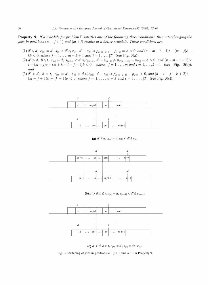
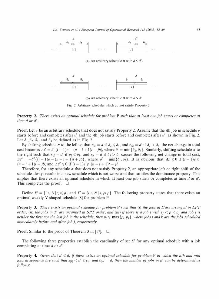
Property 9. If a schedule for problem P satisfies one of the following three conditions, then interchanging thejobs in positions ðm� jþ 1Þ and ðmþ iÞ results in a better schedule. These conditions are:

(1) d 06 d; c½m� ¼ d; s½k� < d 0

6 c½k�; d 0 � s½k� P pE0 ½m�jþ1� � pT 0 ½i� ¼ D > 0; and ðn� m� iþ 1Þt � ðm� jÞe �kb < 0; where j ¼ 1; . . . ;m� k þ 1 and i ¼ 1; . . . ; jT 0j (see Fig. 3(a));

(2) d 0 > d; b6 t; c½m� ¼ d; s½mþk� < d 06 c½mþk�; d 0 � s½mþk� P pE0 ½m�jþ1� � pT 0 ½i� ¼ D > 0; and ðn�m� iþ 1Þ�

t � ðm� jÞe� ðmþ k � i� jþ 1Þb < 0; where j ¼ 1; . . . ;m and i ¼ 1; . . . ; k � 1 (see Fig. 3(b));and

(3) d 0 > d; b > t; c½m� ¼ d 0; s½k� < d 6 c½k�; d � s½k� P pE0 ½m�jþ1� � pT 0 ½i� > 0; and ðn � i � j � k þ 2Þt �ðm � j þ 1Þb � ðk � 1Þe < 0; where j ¼ 1; . . . ; m � k and i ¼ 1; . . . ; jT 0j (see Fig. 3(c)).

Fig. 3. Switching of jobs in positions m� jþ 1 and mþ i in Property 9.


Proof. (1) Consider a schedule r where d 06 d; c½m� ¼ d; s½k� < d 0

6 c½k�, and d 0 � s½k� P pE0 ½m�jþ1� � pT 0 ½i� > 0. Anew schedule r0 can be constructed by interchanging the jobs in positions ðm� jþ 1Þ and ðmþ iÞ and rightshifting all jobs between these two by D, as shown in Fig. 3(a). Then, the difference between the objectivefunctions of schedules r and r0 can be computed as zðr0Þ � zðrÞ ¼ Dfðn� m� iþ 1Þt � ðm� jÞe� kbg < 0.Thus, the new schedule r0 is better than schedule r.The proofs for Conditions (2) and (3) follow similar arguments. �

In contrast to Property 9, the following property states the cases where decreasing the start times of somejobs in sets E0 and T 0 results in an improved schedule.

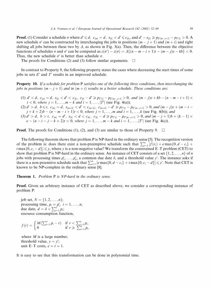
Property 10. If a schedule for problem P satisfies one of the following three conditions, then interchanging thejobs in positions ðm� jþ 1Þ and in ðmþ iÞ results in a better schedule. These conditions are:

(1) d 0 < d; c½m� ¼ d; s½k� < d 0 < c½k�; c½k� � d 0 P pT 0 ½i� � pE0 ½m�jþ1� > 0; and ðm� jÞeþ kb� ðn�m� iþ 1Þ�t < 0; where j ¼ 1; . . . ;m� k and i ¼ 1; . . . ; jT 0j (see Fig. 4(a));

(2) d 0 > d; b6 t; c½m� ¼ d; s½mþk� < d 0 < c½mþk�; c½mþk� � d 0 P pT 0 ½i� � pE0 ½m�jþ1� > 0; and ðm� jÞeþ ðm� i �jþ k þ 2Þb� ðn� m� iþ 1Þt < 0; where j ¼ 1; . . . ;m and i ¼ 1; . . . ; k (see Fig. 4(b)); and

(3) d 0 > d; b > t; c½m� ¼ d 0; s½k� < d < c½k�; c½k� � d P pT 0 ½i� � pE0 ½m�jþ1� > 0; and ðm � j þ 1Þb þ ðk � 1Þ �e � ðn � i � j � k þ 2Þt < 0; where j ¼ 1; . . . ;m � k and i ¼ 1; . . . ; jT 0j (see Fig. 4(c)).

Proof. The proofs for Conditions (1), (2), and (3) are similar to those of Property 9. �

The following theorem shows that problem P is NP-hard in the ordinary sense [5]. The recognition versionof the problem is: does there exist a non-preemptive schedule such that

Pni¼1 ½f ðriÞ þ emaxf0; d � cig þ

tmaxf0; ci � dg�6 y, where y is a non-negative value? We transform the constrained E–T problem (CET) toshow that problem P is NP-hard in the ordinary sense. An instance of CET consists of a set f1; 2; . . . ; ng of njobs with processing times p01; . . . ; p

0n, a common due date d, and a threshold value y0. The instance asks if

there is a non-preemtive schedule such thatPn

i¼1 ½emaxf0; d � cig þ tmaxf0; ci � dg�6 y0. Note that CET isknown to be NP-complete in the ordinary sense [8].

Theorem 1. Problem P is NP-hard in the ordinary sense.

Proof. Given an arbitrary instance of CET as described above, we consider a corresponding instance ofproblem P:

job set, N ¼ f1; 2; . . . ; ng;processing time, pi ¼ p0i; i ¼ 1; . . . ; n;due date, d ¼ d þ

Pni¼1 pi;

resource consumption function,

f ðrÞ ¼ MðPn

i¼1 pi � rÞ if r <Pn

i¼1 pi;0 if rP

Pni¼1 pi;

�

where M is a large number;threshold value, y ¼ y 0;unit E–T costs, e ¼ t ¼ 1.

It is easy to see that this transformation can be done in polynomial time.


Suppose that there is a schedule for CET with total E–T cost no greater than y 0. Then, it is easyto see that an optimal solution to problem P will not start earlier than time

Pni¼1 pi; and hence, mini-

mizing the total resource consumption and E–T penalties is equivalent to solving the given CETproblem.Conversely, suppose there exists a schedule for problem P with the total resource consumption and E–T

penalties no greater than y. Then, it is easy to see that an optimal solution to problem P will not start earlierthan time

Pni¼1 pi; and hence, minimizing the total E–T cost is equivalent to solving the given problem P.

This completes the proof. �

Fig. 4. Switching of jobs in positions m� jþ 1 and mþ i in Property 10.


3. Algorithms

In this section, a polynomial time algorithm is presented to find a heuristic solution to problem P.All the dominance properties presented in the previous section are put together to derive the heuristicalgorithm. A DP algorithm is also presented to find an optimal schedule for small and medium sizeproblems.

3.1. Heuristic algorithm

The heuristic algorithm includes three procedures (Procedures 1–3), which generate schedules based onthe necessary optimality conditions stated in Properties 4–6, respectively. These optimality conditions holdunder certain assumptions. The purpose of the three procedures is to obtain good initial solutions for theheuristic algorithm. In these procedures, w½i� is the resource consumption and E–T cost tentatively assignedto the job placed in the ith position of the schedule being generated, and x½i� represents the set membershipof that job. That is, if x½i� is one (zero), then the job in the ith position is assigned to set E0 (set T 0). Asequence can be determined by assigning the job with the smallest processing time to the largest value ofw½i�, the next smallest job to the next largest w½i�, and so on. From this sequence, a schedule can be con-structed by determining the start times and completion times of the jobs since jE0j defined as m, is deter-mined by x½i�, for i ¼ 1; . . . ; n, and c½m� ¼ q by assumption.The detailed steps of each procedure are presented below. It is assumed that jobs are arranged in non-

decreasing order of their processing times. Throughout these procedures, k is a given value that indicatesthe position of the job that satisfies the condition s½k� < d 0

6 c½k� in Procedure 1, s½mþk� < d 06 c½mþk� in Pro-

cedure 2, or s½k� 6 d < c½k� in Procedure 3 in the schedule that is being generated.

Procedure 1 (for the case d 0 6 d).Step 1. Calculate

w½i� ¼ min

ibþ ði� 1Þe for 16 i6 k;

kbþ ði� 1Þe for k < i6 n;

ðn� iþ 1Þt for 16 i6 n:

8><>:

x½i� ¼ 1 if ibþ ði� 1Þe6 ðn� iþ 1Þt for 16 i6 k; or if kbþ ði� 1Þe6 ðn� iþ 1Þt for k < i6 n;0 otherwise:

�

Step 2. Rank fw½i� j i ¼ 1; . . . ; ng in non-increasing order, where ties are broken by placing the largerindex i first.Obtain schedule rk by assigning job j to position i, where i is the index of w½i� and j is the rank ofw½i�.

Step 3. Determine the job completion time of each job in schedule rk as follows:

m ¼ jEkj ¼ x½1� þ þ x½n�; ck½m� ¼ d; ck½i� ¼ d � pk½iþ 1� � � pk½m�; i ¼ 1; . . . ;m� 1;

and

ck½j� ¼ d þ pk½j� þ pk½j�1� þ þ pk½mþ 1�; j ¼ mþ 1; . . . ; n:

Stop.


Procedure 2 (for the case d 0 > d and b6 t).Step 1. Calculate m ¼ jEkj ¼ dðnt � kbÞ=ðeþ t þ bÞe.

w½i� ¼ min

ibþ ði� 1Þe for 16 i6m;

ðn� iþ 1Þt � ðmþ k � iÞb for mþ 16 i6mþ k;

ðn� iþ 1Þt for mþ k < i6 n:

8><>:

Step 2. Same as Step 2 of Procedure 1.Step 3. Determine the completion time of each job in schedule rk as follows:

ck½m� ¼ d; ck½i� ¼ d � pk½iþ1� � � pk½m�; i ¼ 1; . . . ;m� 1;

and

ck½mþj� ¼ d þ pk½mþ1� þ þ pk½mþj�; j ¼ 1; . . . ; n� m:

Stop.

Procedure 3 (for the case d 0 > d and b > t).Step 1. Calculate

w½i� ¼ min

ibþ ði� 1Þe for 16 i6 k;ibþ ðk � 1Þe� ði� kÞt for k < i6 n;ðn� iþ 1Þt for 16 i6 n:

8<:

x½i� ¼ 1 if ibþ ði� 1Þe6 ðn� iþ 1Þt for 16 i< k;or if ibþ ðk� 1Þe� ði� kÞt6 ðn� iþ 1Þt for k < i6n0 otherwise:

�

Step 2. Same as Step 2 of Procedure 1.Step 3. Determine the completion time of each job in schedule rk as follows:

m ¼ jEkj ¼ x½1� þ þ x½n�; ck½m� ¼ d 0; ck½i� ¼ d 0 � pk½iþ1� � � pk½m�; i ¼ 1; . . . ;m� 1;

and

ck½j� ¼ d 0 þ pk½i� þ pk½i�1� þ þ pk½mþ1�; j ¼ mþ 1; ; n:Stop.

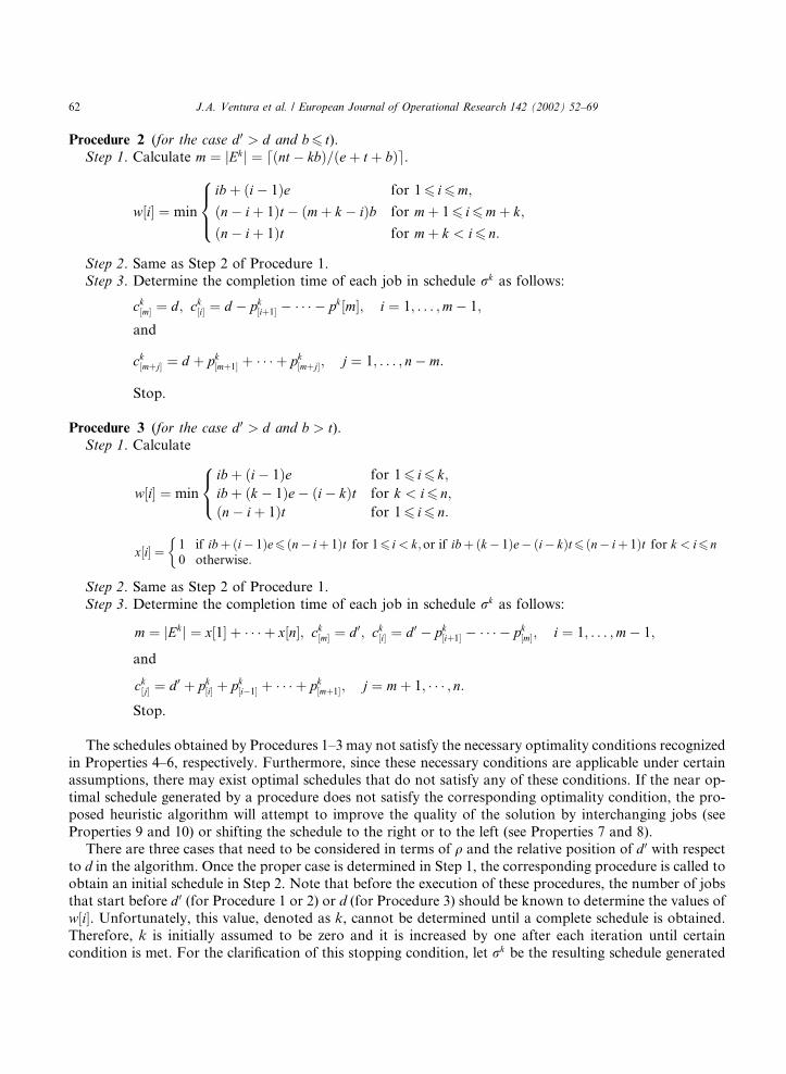
The schedules obtained by Procedures 1–3 may not satisfy the necessary optimality conditions recognizedin Properties 4–6, respectively. Furthermore, since these necessary conditions are applicable under certainassumptions, there may exist optimal schedules that do not satisfy any of these conditions. If the near op-timal schedule generated by a procedure does not satisfy the corresponding optimality condition, the pro-posed heuristic algorithm will attempt to improve the quality of the solution by interchanging jobs (seeProperties 9 and 10) or shifting the schedule to the right or to the left (see Properties 7 and 8).There are three cases that need to be considered in terms of q and the relative position of d 0 with respect

to d in the algorithm. Once the proper case is determined in Step 1, the corresponding procedure is called toobtain an initial schedule in Step 2. Note that before the execution of these procedures, the number of jobsthat start before d 0 (for Procedure 1 or 2) or d (for Procedure 3) should be known to determine the values ofw½i�. Unfortunately, this value, denoted as k, cannot be determined until a complete schedule is obtained.Therefore, k is initially assumed to be zero and it is increased by one after each iteration until certaincondition is met. For the clarification of this stopping condition, let rk be the resulting schedule generated


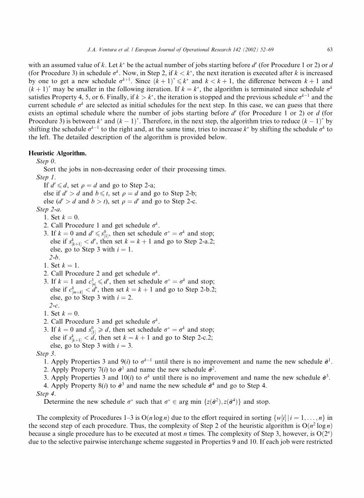
with an assumed value of k. Let k� be the actual number of jobs starting before d 0 (for Procedure 1 or 2) or d(for Procedure 3) in schedule rk. Now, in Step 2, if k < k�, the next iteration is executed after k is increasedby one to get a new schedule rkþ1. Since ðk þ 1Þ� 6 k� and k < k þ 1, the difference between k þ 1 andðk þ 1Þ� may be smaller in the following iteration. If k ¼ k�, the algorithm is terminated since schedule rk

satisfies Property 4, 5, or 6. Finally, if k > k�, the iteration is stopped and the previous schedule rk�1 and thecurrent schedule rk are selected as initial schedules for the next step. In this case, we can guess that thereexists an optimal schedule where the number of jobs starting before d 0 (for Procedure 1 or 2) or d (forProcedure 3) is between k� and ðk � 1Þ�. Therefore, in the next step, the algorithm tries to reduce ðk � 1Þ� byshifting the schedule rk�1 to the right and, at the same time, tries to increase k� by shifting the schedule rk tothe left. The detailed description of the algorithm is provided below.

Heuristic Algorithm.

Step 0.Sort the jobs in non-decreasing order of their processing times.

Step 1.If d 0

6 d, set q ¼ d and go to Step 2-a;else if d 0 > d and b6 t, set q ¼ d and go to Step 2-b;else (d 0 > d and b > t), set q ¼ d 0 and go to Step 2-c.

Step 2-a.1. Set k ¼ 0.2. Call Procedure 1 and get schedule rk.3. If k ¼ 0 and d 0

6 s0½1�, then set schedule r� ¼ rk and stop;else if sk½kþ1� < d 0, then set k ¼ k þ 1 and go to Step 2-a.2;else, go to Step 3 with i ¼ 1.2-b.

1. Set k ¼ 1.2. Call Procedure 2 and get schedule rk.3. If k ¼ 1 and c1½n� 6 d 0, then set schedule r� ¼ rk and stop;else if ck½mþk� < d 0, then set k ¼ k þ 1 and go to Step 2-b.2;else, go to Step 3 with i ¼ 2.2-c.

1. Set k ¼ 0.2. Call Procedure 3 and get schedule rk.3. If k ¼ 0 and s0½1� P d, then set schedule r� ¼ rk and stop;else if sk½kþ1� < d, then set k ¼ k þ 1 and go to Step 2-c.2;else, go to Step 3 with i ¼ 3.

Step 3.1. Apply Properties 3 and 9(i) to rk�1 until there is no improvement and name the new schedule rr1.2. Apply Property 7(i) to rr1 and name the new schedule rr2.3. Apply Properties 3 and 10(i) to rk until there is no improvement and name the new schedule rr3.4. Apply Property 8(i) to rr3 and name the new schedule rr4 and go to Step 4.

Step 4.Determine the new schedule r� such that r� 2 arg min fzðrr2Þ; zðrr4Þg and stop.

The complexity of Procedures 1–3 is Oðn log nÞ due to the effort required in sorting fw½i� j i ¼ 1; . . . ; ng inthe second step of each procedure. Thus, the complexity of Step 2 of the heuristic algorithm is Oðn2 log nÞbecause a single procedure has to be executed at most n times. The complexity of Step 3, however, is Oð2nÞdue to the selective pairwise interchange scheme suggested in Properties 9 and 10. If each job were restricted


to be considered only once in the pairwise interchange scheme, then the complexity of Step 3 would bereduced to OðnÞ and the complexity of the heuristic algorithm would become Oðn2 log nÞ.

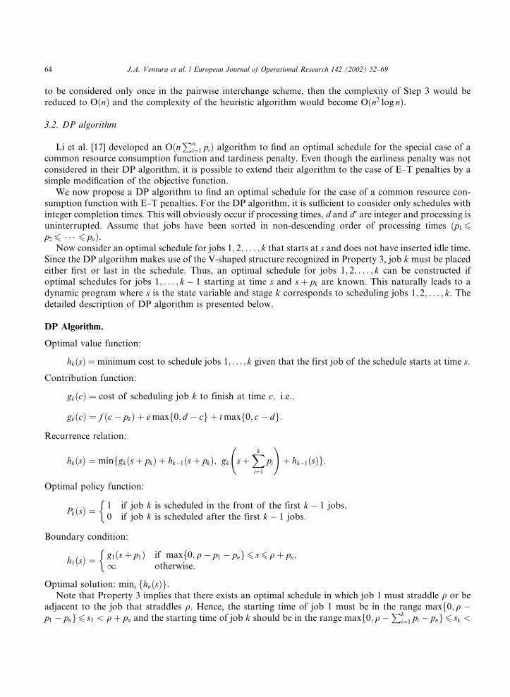
3.2. DP algorithm

Li et al. [17] developed an OðnPn

i¼1 piÞ algorithm to find an optimal schedule for the special case of acommon resource consumption function and tardiness penalty. Even though the earliness penalty was notconsidered in their DP algorithm, it is possible to extend their algorithm to the case of E–T penalties by asimple modification of the objective function.We now propose a DP algorithm to find an optimal schedule for the case of a common resource con-

sumption function with E–T penalties. For the DP algorithm, it is sufficient to consider only schedules withinteger completion times. This will obviously occur if processing times, d and d 0 are integer and processing isuninterrupted. Assume that jobs have been sorted in non-descending order of processing times ðp16p26 6 pnÞ.Now consider an optimal schedule for jobs 1; 2; . . . ; k that starts at s and does not have inserted idle time.

Since the DP algorithm makes use of the V-shaped structure recognized in Property 3, job k must be placedeither first or last in the schedule. Thus, an optimal schedule for jobs 1; 2; . . . ; k can be constructed ifoptimal schedules for jobs 1; . . . ; k � 1 starting at time s and sþ pk are known. This naturally leads to adynamic program where s is the state variable and stage k corresponds to scheduling jobs 1; 2; . . . ; k. Thedetailed description of DP algorithm is presented below.

DP Algorithm.

Optimal value function:

hkðsÞ ¼minimum cost to schedule jobs 1; . . . ; k given that the first job of the schedule starts at time s:

Contribution function:

gkðcÞ ¼ cost of scheduling job k to finish at time c; i:e:;

gkðcÞ ¼ f ðc� pkÞ þ emaxf0; d � cg þ tmaxf0; c� dg:

Recurrence relation:

hkðsÞ ¼ minfgkðsþ pkÞ þ hk�1ðsþ pkÞ; gk s

þXki¼1

pi

!þ hk�1ðsÞg:

Optimal policy function:

PkðsÞ ¼1 if job k is scheduled in the front of the first k � 1 jobs;0 if job k is scheduled after the first k � 1 jobs:

�

Boundary condition:

h1ðsÞ ¼g1ðsþ p1Þ if maxf0; q � p1 � png6 s6 q þ pn;1 otherwise:

�

Optimal solution: mins fhnðsÞg.Note that Property 3 implies that there exists an optimal schedule in which job 1 must straddle q or be

adjacent to the job that straddles q. Hence, the starting time of job 1 must be in the range maxf0; q �p1 � png6 s1 < q þ pn and the starting time of job k should be in the range maxf0; q �

Pki¼1 pi � png6 sk <


q þPk�1

i¼1 pi þ pn. Since k6 n and s is restricted to the range maxf0; q �Pn

i¼1 pig6 s6 q þPn�1

i¼1 pi, thenumber of recurrence relations that must be calculated by the DP algorithm is Oðn

Pni¼1 piÞ. Since f ðrÞ can

be evaluated in constant time, the overall complexity of the DP algorithm is OðnPn

i¼1 piÞ.

3.3. A numerical example

The following step-by-step procedure is provided to illustrate the proposed heuristic algorithm. Givenn ¼ 8 independent jobs with a common due date d ¼ 55. The parameters of the linear resource con-sumption function are given as a ¼ 210 and b ¼ 5. The E–T weights are given as e ¼ 2 and t ¼ 3, re-spectively. The job processing times are provided in Step 0.

Step 0. p1 ¼ 1; p2 ¼ 3; p3 ¼ 6; p4 ¼ 7; p5 ¼ 10; p6 ¼ 13; p7 ¼ 14; p8 ¼ 18.Step 1. Since d 0 ¼ a=b ¼ 42 < d ¼ 55, go to Step 2-a.Step 2-a. Call Procedure 1 with k ¼ 0 (iteration 0).

The resulting schedule r1 is f8; 7; 5; 4; 2 j1; 3; 6g which starts at s0½1� ¼ 3. Since k ¼ 0 and d 0 > s0½1�, go back toStep 2-a and call Procedure 1 to generate the next schedule with k ¼ k þ 1.

Step 2-a. Call Procedure 1 with k ¼ 1 (iteration 1).

The resulting schedule r1 is f7; 5; 3; 2 j1; 4; 6; 8g which starts at s1½1� ¼ 22. Since d 0 > s1½2�, go back to Step 2-awith k ¼ k þ 1.

Step 2-a. Call Procedure 1 with k ¼ 2 (iteration 2).

Position i 1 2 3 4 5 6 7 8

ði� 1Þ e 0 2 4 6 8 10 12 14ðn� iþ 1Þ t 24 21 18 15 12 9 6 3w½i� 0 2 4 6 8 9 6 3x½i� 1 1 1 1 1 0 0 0Rank j 8 7 5 4 2 1 3 6

Position i 1 2 3 4 5 6 7 8

bþ ði� 1Þ e 5 7 9 11 13 15 17 19ðn� iþ 1Þ t 24 21 18 15 12 9 6 3w½i� 5 7 9 11 12 9 6 3x½i� 1 1 1 1 0 0 0 0Rank j 7 5 3 2 1 4 6 8

Position i 1 2 3 4 5 6 7 8

ibþ ði� 1Þ e 5 12 – – – – – –2bþ ði� 1Þ e – – 14 16 18 20 22 24ðn� iþ 1Þ t 24 21 18 15 12 9 6 3w½i� 5 12 14 15 12 9 6 3x½i� 1 1 1 0 0 0 0 0Rank j 7 4 2 1 3 5 6 8


The resulting schedule r2 is f7; 4; 2 j1; 3; 5; 6; 8g which starts at s2½1� ¼ 31. Since d 0 < s2½3�, go to Step 3 withi ¼ 1.

Step 3.

1. Apply Properties 3 and 9(1) to r1 and the resulting schedule rr1 is f7; 5; 2; 1 j3; 4; 6; 8g, which starts atss1½1� ¼ 27. The total cost of schedule rr1 is 385.

2. Apply Property 7(1) to rr1. The new schedule rr2 is the result of shifting the schedule rr1 to the right by 1unit with total cost 384.

3. Apply Properties 3 and 10(1) to r2. From schedule r2, the 3rd and 5th jobs are interchanged and the totalcost of the new schedule rr3 is 381.

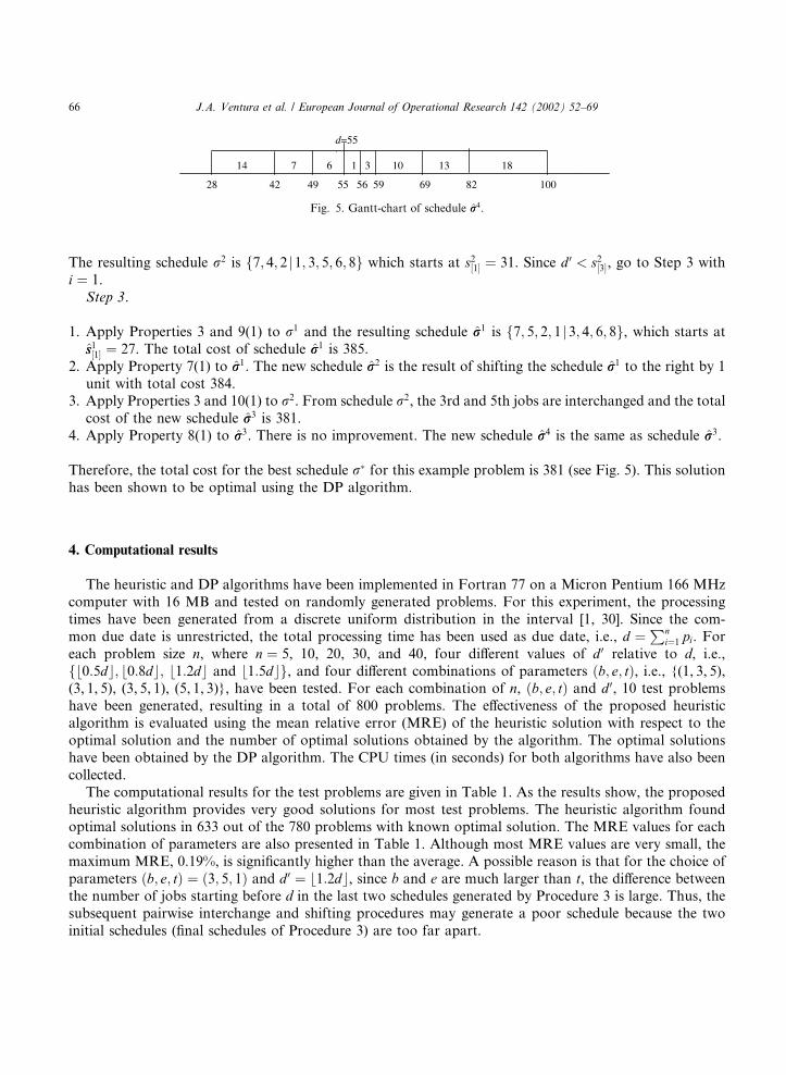
4. Apply Property 8(1) to rr3. There is no improvement. The new schedule rr4 is the same as schedule rr3.

Therefore, the total cost for the best schedule r� for this example problem is 381 (see Fig. 5). This solutionhas been shown to be optimal using the DP algorithm.

4. Computational results

The heuristic and DP algorithms have been implemented in Fortran 77 on a Micron Pentium 166 MHzcomputer with 16 MB and tested on randomly generated problems. For this experiment, the processingtimes have been generated from a discrete uniform distribution in the interval [1, 30]. Since the com-mon due date is unrestricted, the total processing time has been used as due date, i.e., d ¼

Pni¼1 pi. For

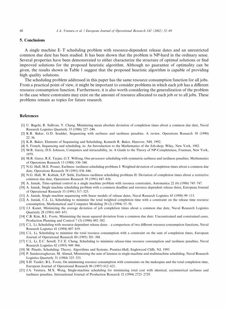
each problem size n, where n ¼ 5, 10, 20, 30, and 40, four different values of d 0 relative to d, i.e.,fb0:5dc; b0:8dc; b1:2dc and b1:5dcg, and four different combinations of parameters ðb; e; tÞ, i.e., {(1, 3, 5),(3, 1, 5), (3, 5, 1), (5, 1, 3)}, have been tested. For each combination of n, ðb; e; tÞ and d 0, 10 test problemshave been generated, resulting in a total of 800 problems. The effectiveness of the proposed heuristicalgorithm is evaluated using the mean relative error (MRE) of the heuristic solution with respect to theoptimal solution and the number of optimal solutions obtained by the algorithm. The optimal solutionshave been obtained by the DP algorithm. The CPU times (in seconds) for both algorithms have also beencollected.The computational results for the test problems are given in Table 1. As the results show, the proposed

heuristic algorithm provides very good solutions for most test problems. The heuristic algorithm foundoptimal solutions in 633 out of the 780 problems with known optimal solution. The MRE values for eachcombination of parameters are also presented in Table 1. Although most MRE values are very small, themaximum MRE, 0.19%, is significantly higher than the average. A possible reason is that for the choice ofparameters ðb; e; tÞ ¼ ð3; 5; 1Þ and d 0 ¼ b1:2dc, since b and e are much larger than t, the difference betweenthe number of jobs starting before d in the last two schedules generated by Procedure 3 is large. Thus, thesubsequent pairwise interchange and shifting procedures may generate a poor schedule because the twoinitial schedules (final schedules of Procedure 3) are too far apart.

Fig. 5. Gantt-chart of schedule rr4.


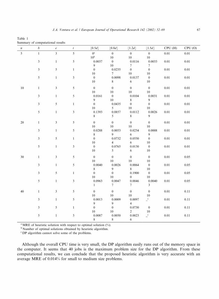
Although the overall CPU time is very small, the DP algorithm easily runs out of the memory space inthe computer. It seems that 40 jobs is the maximum problem size for the DP algorithm. From thesecomputational results, we can conclude that the proposed heuristic algorithm is very accurate with anaverage MRE of 0.014% for small to medium size problems.

Table 1

Summary of computational results

n b e t b0:5dc b0:8dc b1:2dc b1:5dc CPU (H) CPU (O)

5 1 3 5 0a 0 0 0 0.01 0.01

10b 10 10 10

3 1 5 0.0037 0 0.0116 0.0033 0.01 0.01

9 10 7 7

3 5 1 0 0.0235 0 0 0.01 0.01

10 7 10 10

5 1 3 0 0.0098 0.0137 0 0.01 0.01

10 8 6 10

10 1 3 5 0 0 0 0 0.01 0.01

10 10 10 10

3 1 5 0.0161 0 0.0104 0.0031 0.01 0.01

9 10 8 9

3 5 1 0 0.0435 0 0 0.01 0.01

10 5 10 10

5 1 3 0.1393 0.0857 0.0112 0.0026 0.01 0.01

8 5 8 9

20 1 3 5 0 0 0 0 0.01 0.01

10 10 10 10

3 1 5 0.0288 0.0053 0.0254 0.0008 0.01 0.01

8 9 6 9

3 5 1 0 0.0732 0.0550 0 0.01 0.01

10 4 6 10

5 1 3 0 0.0765 0.0130 0 0.01 0.01

10 5 6 10

30 1 3 5 0 0 0 0 0.01 0.05

10 10 10 10

3 1 5 0.0040 0.0026 0.0064 0 0.01 0.05

8 9 8 10

3 5 1 0 0 0.1900 0 0.01 0.05

10 10 0 10

5 1 3 0.0963 0.0047 0.0046 0.0040 0.01 0.05

1 7 7 3

40 1 3 5 0 0 0 0 0.01 0.11

10 10 10 10

3 1 5 0.0013 0.0009 0.0097 _c 0.01 0.11

9 9 4

3 5 1 0 0 0.0730 0 0.01 0.11

10 10 2 10

5 1 3 0.0087 0.0050 0.0023 _c 0.01 0.11

8 8 6

aMRE of heuristic solution with respect to optimal solution (%).bNumber of optimal solutions obtained by heuristic algorithm.cDP algorithm cannot solve some of the problems.


5. Conclusions

A single machine E–T scheduling problem with resource-dependent release dates and an unrestrictedcommon due date has been studied. It has been shown that the problem is NP-hard in the ordinary sense.Several properties have been demonstrated to either characterize the structure of optimal solutions or findimproved solutions for the proposed heuristic algorithm. Although no guarantee of optimality can begiven, the results shown in Table 1 suggest that the proposed heuristic algorithm is capable of providinghigh quality solutions.The scheduling problem addressed in this paper has the same resource consumption function for all jobs.

From a practical point of view, it might be important to consider problems in which each job has a differentresource consumption function. Furthermore, it is also worth considering the generalization of the problemto the case where constraints may exist on the amount of resource allocated to each job or to all jobs. Theseproblems remain as topics for future research.

References

[1] U. Bagchi, R. Sullivan, Y. Chang, Minimizing mean absolute deviation of completion times about a common due date, Naval

Research Logistics Quarterly 33 (1986) 227–240.

[2] K.R. Baker, G.D. Scudder, Sequencing with earliness and tardiness penalties. A review, Operations Research 38 (1990)

22–36.

[3] K.R. Baker, Elements of Sequencing and Scheduling, Kenneth R. Baker, Hanover, NH, 1992.

[4] S. French, Sequencing and scheduling, in: An Introduction to the Mathematics of the Job-shop, Wiley, New York, 1982.

[5] M.R. Garey, D.S. Johnson, Computers and intractability, in: A Guide to the Theory of NP-Completeness, Freeman, New York,

1979.

[6] M.R. Garey, R.E. Tarjan, G.T. Wilfong, One-processor scheduling with symmetric earliness and tardiness penalties, Mathematics

of Operations Research 13 (1988) 330–348.

[7] N.G. Hall, M.E. Posner, Earliness–tardiness scheduling problems I: Weighted deviation of completion times about a common due

date, Operations Research 39 (1991) 836–846.

[8] N.G. Hall, W. Kubiak, S.P. Sethi, Earliness–tardiness scheduling problems II: Deviation of completion times about a restrictive

common due date, Operations Research 39 (1991) 847–856.

[9] A. Janiak, Time-optimal control in a single machine problem with resource constraints, Automatica 22 (6) (1986) 745–747.

[10] A. Janiak, Single machine scheduling problem with a common deadline and resource dependent release dates, European Journal

of Operational Research 53 (1991) 317–325.

[11] A. Janiak, Single machine sequencing with linear models of release dates, Naval Research Logistics 45 (1998) 99–113.

[12] A. Janiak, C.L. Li, Scheduling to minimize the total weighted completion time with a constraint on the release time resource

consumption, Mathematical and Computer Modeling 20 (2) (1994) 53–58.

[13] J.J. Kanet, Minimizing the average deviation of job completion times about a common due date, Naval Research Logistics

Quarterly 28 (1981) 643–651.

[14] C.B. Kim, B.L. Foote, Minimizing the mean squared deviation from a common due date: Unconstrained and constrained cases,

Production Planning and Control 7 (5) (1996) 492–502.

[15] C.L. Li, Scheduling with resource dependent release dates – a comparison of two different resource consumption functions, Naval

Research Logistics 41 (1994) 807–819.

[16] C.L. Li, Scheduling to minimize the total resource consumption with a constraint on the sum of completion times, European

Journal of Operational Research 80 (1995) 381–388.

[17] C.L. Li, E.C. Sewell, T.C.E. Cheng, Scheduling to minimize release-time resource consumption and tardiness penalties, Naval

Research Logistics 42 (1995) 949–966.

[18] M. Pinedo, Scheduling: Theory, Algorithms and Systems, Prentice-Hall, Englewood Cliffs, NJ, 1995.

[19] P. Sundararaghavan, M. Ahmed, Minimizing the sum of lateness in single-machine and multimachine scheduling, Naval Research

Logistics Quarterly 31 (1984) 325–333.

[20] S.H. Vasilev, B.L. Foote, On minimizing resource consumption with constraints on the makespan and the total completion time,

European Journal of Operational Research 96 (1997) 612–621.

[21] J.A. Ventura, M.X. Weng, Single-machine scheduling for minimizing total cost with identical, asymmetrical earliness and

tardiness penalties, International Journal of Production Research 32 (1994) 2725–2729.


[22] J.A. Ventura, M.X. Weng, An improved dynamic programming algorithm for the single-machine mean absolute deviation

problem with a restrictive common due date, Operations Research Letters 17 (1995) 149–152.

[23] M.X. Weng, J.A. Ventura, Scheduling about a large common due date with tolerance to minimize the mean absolute deviation of

completion times, Naval Research Logistics 14 (1994) 843–851.


Documents

Single machine earliness–tardiness scheduling with resource-dependent release dates