Embed Size (px)
Citation preview
Optim LettDOI 10.1007/s11590-012-0494-4
ORIGINAL PAPER
Single machine scheduling with sum-of-logarithm-processing-times based and position based learning effects
Ji-Bo Wang · Jian-Jun Wang
Received: 22 September 2011 / Accepted: 16 April 2012© Springer-Verlag 2012
Abstract In this paper we consider the single machine scheduling problems withsum-of-logarithm-processing-times based and position based learning effects, i.e., theactual job processing time of a job is a function of the sum of the logarithms ofthe processing times of the jobs already processed and its position in a sequence. Thelogarithm function is used to model the phenomenon that learning as a human activityis subject to the law of diminishing return. We show that even with the introduction ofthe proposed model to job processing times, several single machine problems remainpolynomially solvable.
Keywords Scheduling · Single machine · Learning effect
1 Introduction
In classical scheduling problems, the processing times of jobs are assumed to beconstant values. However, in many/various practical/real life settings/applications,both machines and workers can improve their performance by repeating the pro-duction operations. Therefore, the actual processing time of a job is shorter if it isscheduled later in a sequence. This phenomenon is known as the “learning effect” inthe literature [1].
J.-B. Wang (B)School of Science, Shenyang Aerospace University, Shenyang 110136, Chinae-mail: [email protected]
J.-J. WangFaculty of Management and Economics, Dalian University of Technology,Dalian 116024, China
123
J.-B. Wang, J.-J. Wang
Biskup [2] and Cheng and Wang [4] were among the pioneers that brought theconcept of learning into the field of scheduling, although it has been widely employedin management science since its discovery by Wright [24]. Biskup [2] proved thatsingle-machine scheduling with a learning effect remains polynomially solvable ifthe objective is to minimize the deviation from a common due date or to minimizethe sum of flow time. Cheng and Wang [4] considered a single machine schedulingproblem in which the job processing times decrease as a result of learning. A volume-dependent piecewise linear processing time function was used to model the learningeffects. The objective was to minimize the maximum lateness. They showed that theproblem is NP-hard in the strong sense and then identified two special cases which arepolynomially solvable. They also proposed two heuristics and analysed their worst-case performance. An extensive survey of different scheduling models and problemswith learning effects could be found in [3]. More recent papers which have consideredscheduling jobs with learning effects include [5–8,10–14,17–23,25–29].
However, the actual processing time of a given job drops to zero precipitously asthe number of jobs increases in the first model and when the normal job processingtimes are large in the second model classified in [3]. Motivated by this observation,we propose a new learning model where the actual job processing time is a functionof the sum of the logarithm of the processing times of the jobs already processed. Thismodel is adopted from [7,29]. The remaining part of this note is organized as follows.In Sect. 2, we formulate the model. In Sect. 3, we consider several single machinescheduling problems. The last section presents the conclusions.
2 Problems description
We formulate the problem as follows: There are n jobs J1, J2, . . ., Jn to be processedon a single machines. The machine can handle one job at a time and preemption isnot allowed. All jobs are available for processing at time zero. The normal processingtime of job J j is denoted by p j with ln p j ≥ 1. Let p j[r ] be the actual processingtime of job J j if it is scheduled in position r in a sequence. Cheng et al. [7] consideredthe following single machine model, i.e., the actual processing time of job J j if it isscheduled in the r th position in a sequence is p j[r ] = p j (1 + ∑r−1
i=1 ln p[i])a, wherep[i] denotes the normal processing time of job scheduled in the i th position in thesequence, and a ≤ 0 is the learning index. Zhang et al. [29] considered the model
where processing time of job J j is p j[r ] = pi j qa1r (c −
∑r−1l=1 βl pi[l]∑n
l=1 pil)a2 , where a1 < 0
and a2 ≥ 1 are the learning indices. In this paper, we propose a new model that stemsfrom [7,29]. Specially, the actual processing time of job J j if it is scheduled in ther th position in a sequence is The actual processing time of job J j ( j = 1, 2, . . ., n) ifscheduled in position r is
p j[r ] = p j qa1r
(
c −∑r−1
l=1 βl ln p[l]∑n
l=1 pl
)a2
, (1)
123
Single machine scheduling with sum-of-logarithm-processing
where p[l] is the normal processing time of a job if it is scheduled in the lth positionin a sequence, c > 0 is a constant and ∀r,
∑r−1l=1 βl ln p[l] ≤ c
∑nl=1 pl , qr is a
non-decreasing function of the scheduled position, i.e. 0 ≤ q1 ≤ q2 ≤ · · · ≤ qn , βl isa non-decreasing sequence of coefficients, i.e. 0 ≤ β1 ≤ β2 ≤ · · · ≤ βn ≤ 1, a1 < 0and a2 ≥ 1 are the learning indices.
For a given schedule π , let C j = C j (π) denote the completion time of job J j . In thispaper we will consider the minimization of the following objective functions: the make-span Cmax = max{C j | j = 1, 2, . . . , n}, the total completion time
∑C j , the total late-
ness∑
L j , the sum of the θ th (θ ≥ 0) power of job completion times∑
Cθj , the total
weighted completion time∑
w j C j , the discounted total weighted completion time∑nj=1 w j (1−e−γ C j ) , the maximum lateness Lmax = max{C j −d j | j = 1, 2, . . . , n},
the maximum tardiness Tmax = max{0, L j | j = 1, 2, . . . , n} and the total tardiness∑Tj , where w j and d j denote the weight and due date of job J j , L j = C j − d j
and γ ∈ (0, 1) is the discount factor (see [15], Section 3.1). In the remaining part ofthe paper, all the problems considered will be denoted using the three-field notationscheme α|β|γ introduced by [9].
3 Several single machine scheduling problems
First, we give some lemmas, they are useful for the following theorems (the proofs ofthe lemmas are given in the Appendix).
Lemma 1 q(1 − δ)a2 + qδa2(1 − δ)a2−1 − 1 ≤ 0 if 0 < δ ≤ 1, 0 < q ≤ 1 anda2 ≥ 1.
Lemma 2 q(1 − δx)a2 +qδa2(1 − δx)a2−1 − 1 ≤ 0 if 0 < δ ≤ 1, a2 ≥ 1, 0 < q ≤ 1and x ≥ 1.
Lemma 3 (1 − λ) + λq(1 − δx)a2 − q(1 − δ ln λ − δx)a2 ≤ 0 for λ ≥ 1, 0 < δ ≤1, a2 ≥ 1, 0 < q ≤ 1 and x ≥ 1.
Theorem 1 For the problem 1|p j[r ] = p j qa1r (c −
∑r−1l=1 βl ln p[l]∑n
l=1 pl)a2 |Cmax, an optimal
schedule can be obtained by sequencing the jobs in non-decreasing order of p j (theSPT rule).
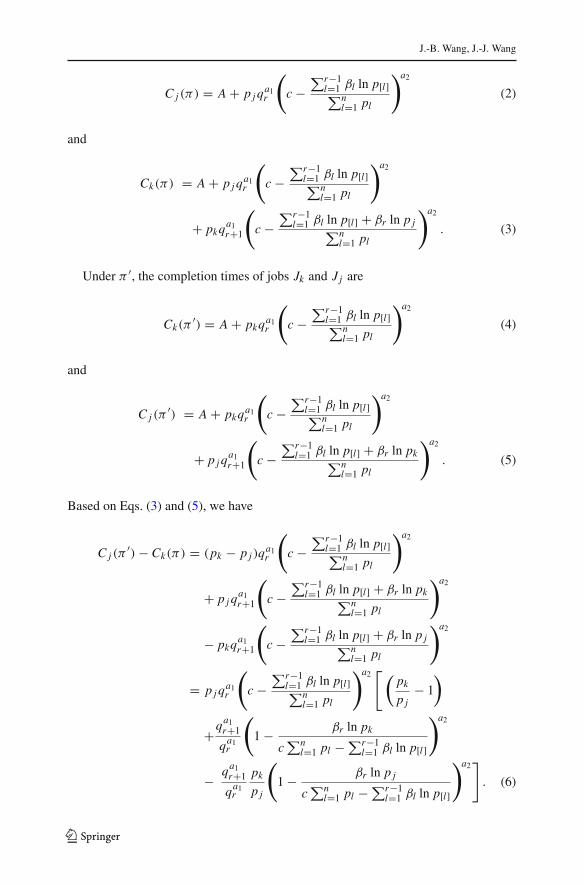
Proof The proof follows directly from the pairwise interchange analysis. Let π and π ′be two job schedules where the difference between π and π ′ is a pairwise interchangeof two adjacent jobs J j and Jk , that is, π = [S1, J j , Jk, S2], π ′ = [S1, Jk, J j , S2],where S1 and S2 are partial sequences. Furthermore, we assume that there are r − 1jobs in S1. Thus, J j and Jk are the r th and the (r +1)th jobs with p j ≤ pk , respectively,in π . Likewise, Jk and J j are scheduled in the r th and the (r + 1)th positions in π ′.To further simplify the notation, let A denote the completion time of the last job in S1and Jh be the first job in S2. To show π dominates π ′, it suffices to show that the (r+1)thjobs in π and π ′ satisfy the condition that Ck(π) ≤ C j (π
′) and Cu(π) ≤ Cu(π ′) forany Ju in S2. Under π , the completion times of jobs J j and Jk are
123
J.-B. Wang, J.-J. Wang
C j (π) = A + p j qa1r
(
c −∑r−1
l=1 βl ln p[l]∑n
l=1 pl
)a2
(2)
and
Ck(π) = A + p j qa1r
(
c −∑r−1
l=1 βl ln p[l]∑n
l=1 pl
)a2
+ pkqa1r+1
(
c −∑r−1
l=1 βl ln p[l] + βr ln p j∑n
l=1 pl
)a2
. (3)
Under π ′, the completion times of jobs Jk and J j are
Ck(π′) = A + pkqa1
r
(
c −∑r−1
l=1 βl ln p[l]∑n
l=1 pl
)a2
(4)
and
C j (π′) = A + pkqa1
r
(
c −∑r−1
l=1 βl ln p[l]∑n
l=1 pl
)a2
+ p j qa1r+1
(
c −∑r−1
l=1 βl ln p[l] + βr ln pk∑n
l=1 pl
)a2
. (5)
Based on Eqs. (3) and (5), we have
C j (π′) − Ck(π) = (pk − p j )q
a1r
(
c −∑r−1
l=1 βl ln p[l]∑n
l=1 pl
)a2
+ p j qa1r+1
(
c −∑r−1
l=1 βl ln p[l] + βr ln pk∑n
l=1 pl
)a2
− pkqa1r+1
(
c −∑r−1
l=1 βl ln p[l] + βr ln p j∑n
l=1 pl
)a2
= p j qa1r
(
c −∑r−1
l=1 βl ln p[l]∑n
l=1 pl
)a2[ (
pk
p j− 1
)
+qa1r+1
qa1r
(
1 − βr ln pk
c∑n
l=1 pl − ∑r−1l=1 βl ln p[l]
)a2
− qa1r+1
qa1r
pk
p j
(
1 − βr ln p j
c∑n
l=1 pl − ∑r−1l=1 βl ln p[l]
)a2]
. (6)
123
Single machine scheduling with sum-of-logarithm-processing
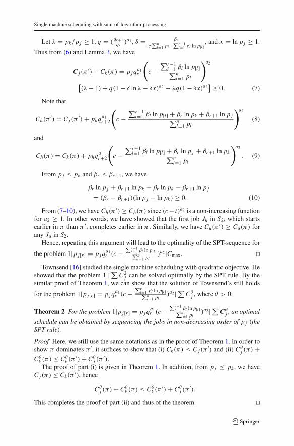
Let λ = pk/p j ≥ 1, q = (qr+1
qr)a1 , δ = βr
c∑n
l=1 pl−∑r−1l=1 βl ln p[l]
, and x = ln p j ≥ 1.
Thus from (6) and Lemma 3, we have
C j (π′) − Ck(π) = p j q
a1r
(
c −∑r−1
l=1 βl ln p[l]∑n
l=1 pl
)a2
[(λ − 1) + q(1 − δ ln λ − δx)a2 − λq(1 − δx)a2
] ≥ 0. (7)
Note that
Ch(π ′) = C j (π′) + phqa1
r+2
(
c −∑r−1
l=1 βl ln p[l] + βr ln pk + βr+1 ln p j∑n
l=1 pl
)a2
(8)
and
Ch(π) = Ck(π) + phqa1r+2
(
c −∑r−1
l=1 βl ln p[l] + βr ln p j + βr+1 ln pk∑n
l=1 pl
)a2
. (9)
From p j ≤ pk and βr ≤ βr+1, we have
βr ln p j + βr+1 ln pk − βr ln pk − βr+1 ln p j
= (βr − βr+1)(ln p j − ln pk) ≥ 0. (10)
From (7–10), we have Ch(π ′) ≥ Ch(π) since (c− t)a2 is a non-increasing functionfor a2 ≥ 1. In other words, we have showed that the first job Jh in S2, which startsearlier in π than π ′, completes earlier in π . Similarly, we have Cu(π ′) ≥ Cu(π) forany Ju in S2.
Hence, repeating this argument will lead to the optimality of the SPT-sequence for
the problem 1|p j[r ] = p j qa1r (c −
∑r−1l=1 βl ln p[l]∑n
l=1 pl)a2 |Cmax. ��
Townsend [16] studied the single machine scheduling with quadratic objective. Heshowed that the problem 1||∑ C2
j can be solved optimally by the SPT rule. By thesimilar proof of Theorem 1, we can show that the solution of Townsend’s still holds
for the problem 1|p j[r ] = p j qa1r (c −
∑r−1l=1 βl ln p[l]∑n
l=1 pl)a2 | ∑ Cθ
j , where θ > 0.
Theorem 2 For the problem 1|p j[r ] = p j qa1r (c −
∑r−1l=1 βl ln p[l]∑n
l=1 pl)a2 | ∑ Cθ
j , an optimal
schedule can be obtained by sequencing the jobs in non-decreasing order of p j (theSPT rule).
Proof Here, we still use the same notations as in the proof of Theorem 1. In order toshow π dominates π ′, it suffices to show that (i) Ck(π) ≤ C j (π
′) and (ii) Cθj (π) +
Cθk (π) ≤ Cθ
k (π ′) + Cθj (π
′).The proof of part (i) is given in Theorem 1. In addition, from p j ≤ pk , we have
C j (π) ≤ Ck(π′), hence
Cθj (π) + Cθ
k (π) ≤ Cθk (π ′) + Cθ
j (π′).
This completes the proof of part (ii) and thus of the theorem. ��
123
J.-B. Wang, J.-J. Wang
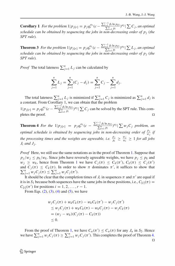
Corollary 1 For the problem 1|p j[r ] = p j qa1r (c −
∑r−1l=1 βl ln p[l]∑n
l=1 pl)a2 | ∑ C j , an optimal
schedule can be obtained by sequencing the jobs in non-decreasing order of p j (theSPT rule).
Theorem 3 For the problem 1|p j[r ] = p j qa1r (c −
∑r−1l=1 βl ln p[l]∑n
l=1 pl)a2 | ∑ L j , an optimal
schedule can be obtained by sequencing the jobs in non-decreasing order of p j (theSPT rule).
Proof The total lateness∑n
j=1 L j can be calculated by
n∑
j=1
L j =n∑
j=1
(C j − d j ) =n∑
j=1
C j −n∑
j=1
d j .
The total lateness∑n
j=1 L j is minimized if∑n
j=1 C j is minimized as∑n
j=1 d j isa constant. From Corollary 1, we can obtain that the problem
1|p j[r ] = p j qa1r (c −
∑r−1l=1 βl ln p[l]∑n
l=1 pl)a2 | ∑ C j can be solved by the SPT rule. This com-
pletes the proof. ��
Theorem 4 For the 1|p j[r ] = p j qa1r (c −
∑r−1l=1 βl ln p[l]∑n
l=1 pl)a2 | ∑w j C j problem, an
optimal schedule is obtained by sequencing jobs in non-decreasing order ofp jw j
if
the processing times and the weights are agreeable, i.e.p jpi
≥ w jwi
≥ 1 for all jobsJi and J j .
Proof Here, we still use the same notations as in the proof of Theorem 1. Suppose thatp j/w j ≤ pk/wk . Since jobs have reversely agreeable weights, we have p j ≤ pk andw j ≥ wk , hence from Theorem 1 we have C j (π) ≤ Ck(π
′), Ck(π) ≤ C j (π′)
and C j (π) ≤ Ck(π). In order to show π dominates π ′, it suffices to show that∑nj=1 w j C j (π) ≤ ∑n
j=1 w j C j (π′).
It should be clear that the completion times of Ji in sequences π and π ′ are equal ifit is in S1 because both sequences have the same jobs in these positions, i.e., C[i](π) =C[i](π ′) for positions i = 1, 2, . . . , r − 1.
From Eqs. (2), (3), (4) and (5), we have
w j C j (π) + wkCk(π) − wkCk(π′) − w j C j (π
′)≤ w j C j (π) + wkCk(π) − wkC j (π) − w j Ck(π)
= (w j − wk)(C j (π) − Ck(π))
≤ 0.
From the proof of Theorem 1, we have Cu(π ′) ≤ Cu(π) for any Ju in S2. Hencewe have
∑nj=1 w j C j (π) ≥ ∑n
j=1 w j C j (π′). This completes the proof of Theorem 4.
��
123
Single machine scheduling with sum-of-logarithm-processing
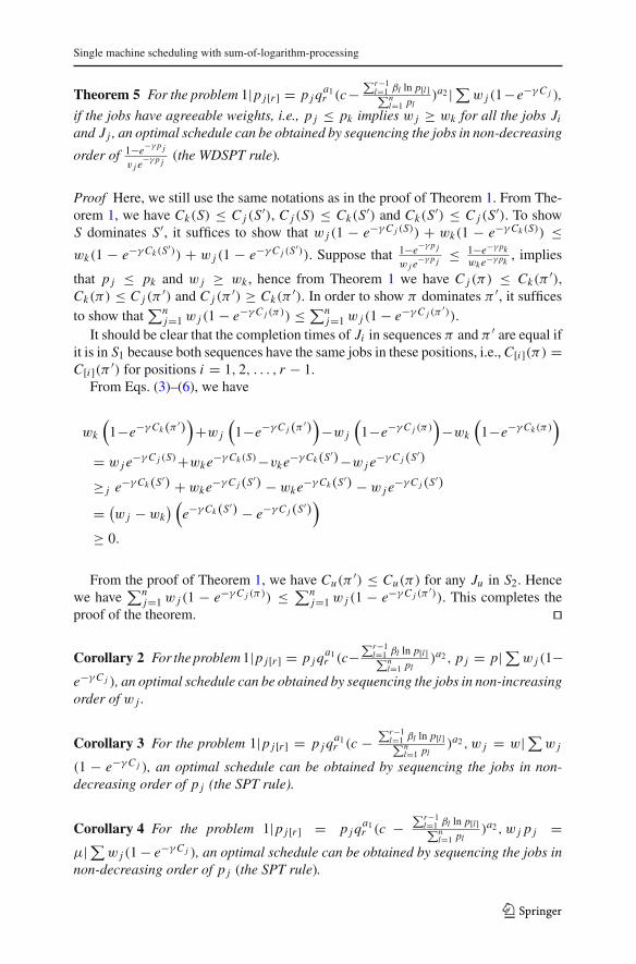
Theorem 5 For the problem 1|p j[r ] = p j qa1r (c−
∑r−1l=1 βl ln p[l]∑n
l=1 pl)a2 | ∑w j (1−e−γ C j ),
if the jobs have agreeable weights, i.e., p j ≤ pk implies w j ≥ wk for all the jobs Ji
and J j , an optimal schedule can be obtained by sequencing the jobs in non-decreasing
order of 1−e−γ p j
v j e−γ p j
(the WDSPT rule).
Proof Here, we still use the same notations as in the proof of Theorem 1. From The-orem 1, we have Ck(S) ≤ C j (S′), C j (S) ≤ Ck(S′) and Ck(S′) ≤ C j (S′). To showS dominates S′, it suffices to show that w j (1 − e−γ C j (S)) + wk(1 − e−γ Ck (S)) ≤wk(1 − e−γ Ck (S′)) + w j (1 − e−γ C j (S′)). Suppose that 1−e−γ p j
w j e−γ p j≤ 1−e−γ pk
wk e−γ pk, implies
that p j ≤ pk and w j ≥ wk , hence from Theorem 1 we have C j (π) ≤ Ck(π′),
Ck(π) ≤ C j (π′) and C j (π
′) ≥ Ck(π′). In order to show π dominates π ′, it suffices
to show that∑n
j=1 w j (1 − e−γ C j (π)) ≤ ∑nj=1 w j (1 − e−γ C j (π
′)).It should be clear that the completion times of Ji in sequences π and π ′ are equal if
it is in S1 because both sequences have the same jobs in these positions, i.e., C[i](π) =C[i](π ′) for positions i = 1, 2, . . . , r − 1.
From Eqs. (3)–(6), we have
wk
(1−e−γ Ck(π ′)
)+w j
(1−e−γ C j (π ′)
)−w j
(1−e−γ C j (π)
)−wk
(1−e−γ Ck (π)
)
= w j e−γ C j (S)+wke−γ Ck (S)−vke−γ Ck(S′)−w j e
−γ C j(S′)
≥ j e−γ Ck(S′) + wke−γ C j(S′) − wke−γ Ck(S′) − w j e−γ C j(S′)
= (w j − wk
) (e−γ Ck(S′) − e−γ C j(S′)
)
≥ 0.
From the proof of Theorem 1, we have Cu(π ′) ≤ Cu(π) for any Ju in S2. Hencewe have
∑nj=1 w j (1 − e−γ C j (π)) ≤ ∑n
j=1 w j (1 − e−γ C j (π′)). This completes the
proof of the theorem. ��
Corollary 2 For the problem 1|p j[r ] = p j qa1r (c−
∑r−1l=1 βl ln p[l]∑n
l=1 pl)a2 , p j = p| ∑w j (1−
e−γ C j ), an optimal schedule can be obtained by sequencing the jobs in non-increasingorder of w j .
Corollary 3 For the problem 1|p j[r ] = p j qa1r (c −
∑r−1l=1 βl ln p[l]∑n
l=1 pl)a2 , w j = w| ∑w j
(1 − e−γ C j ), an optimal schedule can be obtained by sequencing the jobs in non-decreasing order of p j (the SPT rule).
Corollary 4 For the problem 1|p j[r ] = p j qa1r (c −
∑r−1l=1 βl ln p[l]∑n
l=1 pl)a2 , w j p j =
μ| ∑ w j (1 − e−γ C j ), an optimal schedule can be obtained by sequencing the jobs innon-decreasing order of p j (the SPT rule).
123
J.-B. Wang, J.-J. Wang
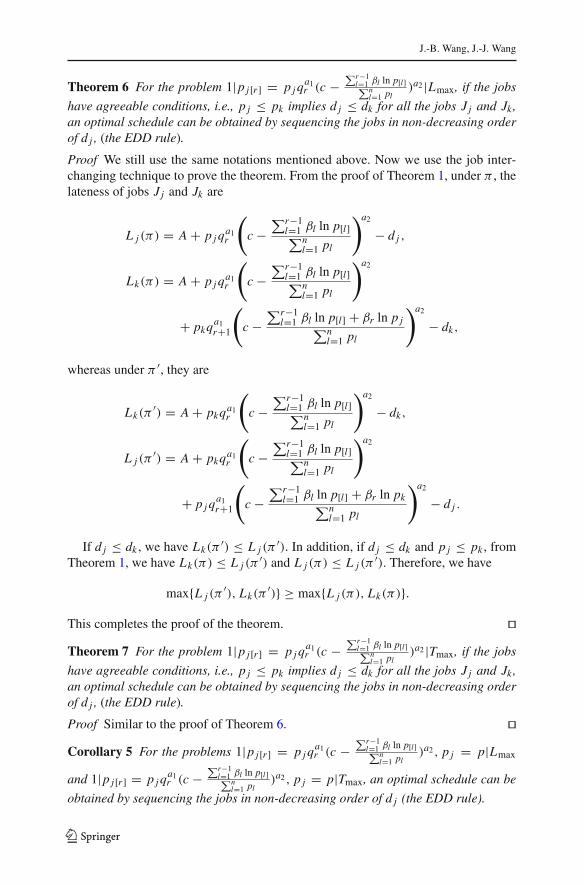
Theorem 6 For the problem 1|p j[r ] = p j qa1r (c −
∑r−1l=1 βl ln p[l]∑n
l=1 pl)a2 |Lmax, if the jobs
have agreeable conditions, i.e., p j ≤ pk implies d j ≤ dk for all the jobs J j and Jk,an optimal schedule can be obtained by sequencing the jobs in non-decreasing orderof d j , (the EDD rule).
Proof We still use the same notations mentioned above. Now we use the job inter-changing technique to prove the theorem. From the proof of Theorem 1, under π , thelateness of jobs J j and Jk are
L j (π) = A + p j qa1r
(
c −∑r−1
l=1 βl ln p[l]∑n
l=1 pl
)a2
− d j ,
Lk(π) = A + p j qa1r
(
c −∑r−1
l=1 βl ln p[l]∑n
l=1 pl
)a2
+ pkqa1r+1
(
c −∑r−1
l=1 βl ln p[l] + βr ln p j∑n
l=1 pl
)a2
− dk,
whereas under π ′, they are
Lk(π′) = A + pkqa1
r
(
c −∑r−1
l=1 βl ln p[l]∑n
l=1 pl
)a2
− dk,
L j (π′) = A + pkqa1
r
(
c −∑r−1
l=1 βl ln p[l]∑n
l=1 pl
)a2
+ p j qa1r+1
(
c −∑r−1
l=1 βl ln p[l] + βr ln pk∑n
l=1 pl
)a2
− d j .
If d j ≤ dk , we have Lk(π′) ≤ L j (π
′). In addition, if d j ≤ dk and p j ≤ pk , fromTheorem 1, we have Lk(π) ≤ L j (π
′) and L j (π) ≤ L j (π′). Therefore, we have
max{L j (π′), Lk(π
′)} ≥ max{L j (π), Lk(π)}.This completes the proof of the theorem. ��Theorem 7 For the problem 1|p j[r ] = p j q
a1r (c −
∑r−1l=1 βl ln p[l]∑n
l=1 pl)a2 |Tmax, if the jobs
have agreeable conditions, i.e., p j ≤ pk implies d j ≤ dk for all the jobs J j and Jk,an optimal schedule can be obtained by sequencing the jobs in non-decreasing orderof d j , (the EDD rule).
Proof Similar to the proof of Theorem 6. ��Corollary 5 For the problems 1|p j[r ] = p j q
a1r (c −
∑r−1l=1 βl ln p[l]∑n
l=1 pl)a2 , p j = p|Lmax
and 1|p j[r ] = p j qa1r (c −
∑r−1l=1 βl ln p[l]∑n
l=1 pl)a2 , p j = p|Tmax, an optimal schedule can be
obtained by sequencing the jobs in non-decreasing order of d j (the EDD rule).
123
Single machine scheduling with sum-of-logarithm-processing
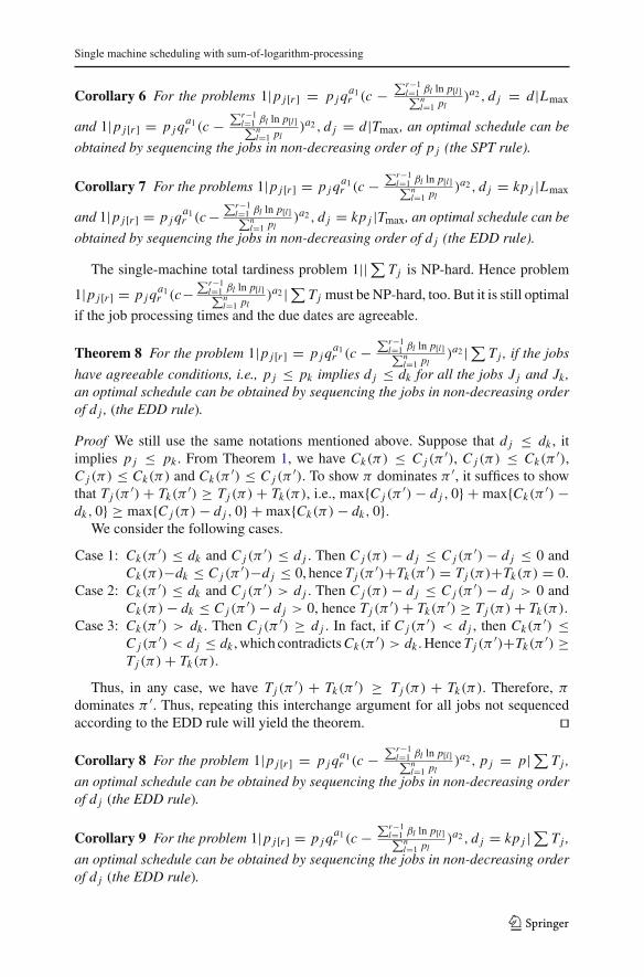
Corollary 6 For the problems 1|p j[r ] = p j qa1r (c −
∑r−1l=1 βl ln p[l]∑n
l=1 pl)a2 , d j = d|Lmax
and 1|p j[r ] = p j qa1r (c −
∑r−1l=1 βl ln p[l]∑n
l=1 pl)a2 , d j = d|Tmax, an optimal schedule can be
obtained by sequencing the jobs in non-decreasing order of p j (the SPT rule).
Corollary 7 For the problems 1|p j[r ] = p j qa1r (c −
∑r−1l=1 βl ln p[l]∑n
l=1 pl)a2 , d j = kp j |Lmax
and 1|p j[r ] = p j qa1r (c −
∑r−1l=1 βl ln p[l]∑n
l=1 pl)a2 , d j = kp j |Tmax, an optimal schedule can be
obtained by sequencing the jobs in non-decreasing order of d j (the EDD rule).
The single-machine total tardiness problem 1||∑ Tj is NP-hard. Hence problem
1|p j[r ] = p j qa1r (c−
∑r−1l=1 βl ln p[l]∑n
l=1 pl)a2 | ∑ Tj must be NP-hard, too. But it is still optimal
if the job processing times and the due dates are agreeable.
Theorem 8 For the problem 1|p j[r ] = p j qa1r (c −
∑r−1l=1 βl ln p[l]∑n
l=1 pl)a2 | ∑ Tj , if the jobs
have agreeable conditions, i.e., p j ≤ pk implies d j ≤ dk for all the jobs J j and Jk,an optimal schedule can be obtained by sequencing the jobs in non-decreasing orderof d j , (the EDD rule).
Proof We still use the same notations mentioned above. Suppose that d j ≤ dk , itimplies p j ≤ pk . From Theorem 1, we have Ck(π) ≤ C j (π
′), C j (π) ≤ Ck(π′),
C j (π) ≤ Ck(π) and Ck(π′) ≤ C j (π
′). To show π dominates π ′, it suffices to showthat Tj (π
′) + Tk(π′) ≥ Tj (π) + Tk(π), i.e., max{C j (π
′) − d j , 0} + max{Ck(π′) −
dk, 0} ≥ max{C j (π) − d j , 0} + max{Ck(π) − dk, 0}.We consider the following cases.
Case 1: Ck(π′) ≤ dk and C j (π
′) ≤ d j . Then C j (π) − d j ≤ C j (π′) − d j ≤ 0 and
Ck(π)−dk ≤ C j (π′)−d j ≤ 0, hence Tj (π
′)+Tk(π′) = Tj (π)+Tk(π) = 0.
Case 2: Ck(π′) ≤ dk and C j (π
′) > d j . Then C j (π) − d j ≤ C j (π′) − d j > 0 and
Ck(π) − dk ≤ C j (π′) − d j > 0, hence Tj (π
′) + Tk(π′) ≥ Tj (π) + Tk(π).
Case 3: Ck(π′) > dk . Then C j (π
′) ≥ d j . In fact, if C j (π′) < d j , then Ck(π
′) ≤C j (π
′) < d j ≤ dk , which contradicts Ck(π′) > dk . Hence Tj (π
′)+Tk(π′) ≥
Tj (π) + Tk(π).
Thus, in any case, we have Tj (π′) + Tk(π
′) ≥ Tj (π) + Tk(π). Therefore, π
dominates π ′. Thus, repeating this interchange argument for all jobs not sequencedaccording to the EDD rule will yield the theorem. ��
Corollary 8 For the problem 1|p j[r ] = p j qa1r (c −
∑r−1l=1 βl ln p[l]∑n
l=1 pl)a2 , p j = p| ∑ Tj ,
an optimal schedule can be obtained by sequencing the jobs in non-decreasing orderof d j (the EDD rule).
Corollary 9 For the problem 1|p j[r ] = p j qa1r (c −
∑r−1l=1 βl ln p[l]∑n
l=1 pl)a2 , d j = kp j | ∑ Tj ,
an optimal schedule can be obtained by sequencing the jobs in non-decreasing orderof d j (the EDD rule).
123
J.-B. Wang, J.-J. Wang
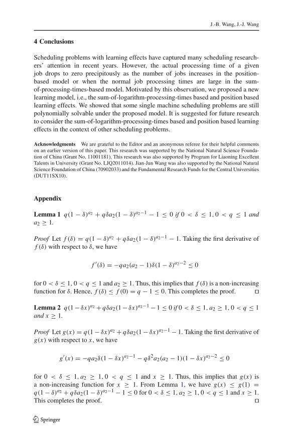
4 Conclusions
Scheduling problems with learning effects have captured many scheduling research-ers’ attention in recent years. However, the actual processing time of a givenjob drops to zero precipitously as the number of jobs increases in the position-based model or when the normal job processing times are large in the sum-of-processing-times-based model. Motivated by this observation, we proposed a newlearning model, i.e., the sum-of-logarithm-processing-times based and position basedlearning effects. We showed that some single machine scheduling problems are stillpolynomially solvable under the proposed model. It is suggested for future researchto consider the sum-of-logarithm-processing-times based and position based learningeffects in the context of other scheduling problems.
Acknowledgments We are grateful to the Editor and an anonymous referee for their helpful commentson an earlier version of this paper. This research was supported by the National Natural Science Founda-tion of China (Grant No. 11001181). This research was also supported by Program for Liaoning ExcellentTalents in University (Grant No. LJQ2011014). Jian-Jun Wang was also supported by the National NaturalScience Foundation of China (70902033) and the Fundamental Research Funds for the Central Universities(DUT11SX10).
Appendix
Lemma 1 q(1 − δ)a2 + qδa2(1 − δ)a2−1 − 1 ≤ 0 if 0 < δ ≤ 1, 0 < q ≤ 1 anda2 ≥ 1.
Proof Let f (δ) = q(1 − δ)a2 + qδa2(1 − δ)a2−1 − 1. Taking the first derivative off (δ) with respect to δ, we have
f ′(δ) = −qa2(a2 − 1)δ(1 − δ)a2−2 ≤ 0
for 0 < δ ≤ 1, 0 < q ≤ 1 and a2 ≥ 1. Thus, this implies that f (δ) is a non-increasingfunction for δ. Hence, f (δ) ≤ f (0) = q − 1 ≤ 0. This completes the proof. ��
Lemma 2 q(1 − δx)a2 +qδa2(1 − δx)a2−1 − 1 ≤ 0 if 0 < δ ≤ 1, a2 ≥ 1, 0 < q ≤ 1and x ≥ 1.
Proof Let g(x) = q(1 − δx)a2 + qδa2(1 − δx)a2−1 − 1. Taking the first derivative ofg(x) with respect to x , we have
g′(x) = −qa2δ(1 − δx)a2−1 − qδ2a2(a2 − 1)(1 − δx)a2−2 ≤ 0
for 0 < δ ≤ 1, a2 ≥ 1, 0 < q ≤ 1 and x ≥ 1. Thus, this implies that g(x) isa non-increasing function for x ≥ 1. From Lemma 1, we have g(x) ≤ g(1) =q(1 − δ)a2 + qδa2(1 − δ)a2−1 − 1 ≤ 0 for 0 < δ ≤ 1, a2 ≥ 1, 0 < q ≤ 1 and x ≥ 1.This completes the proof. ��
123
Single machine scheduling with sum-of-logarithm-processing
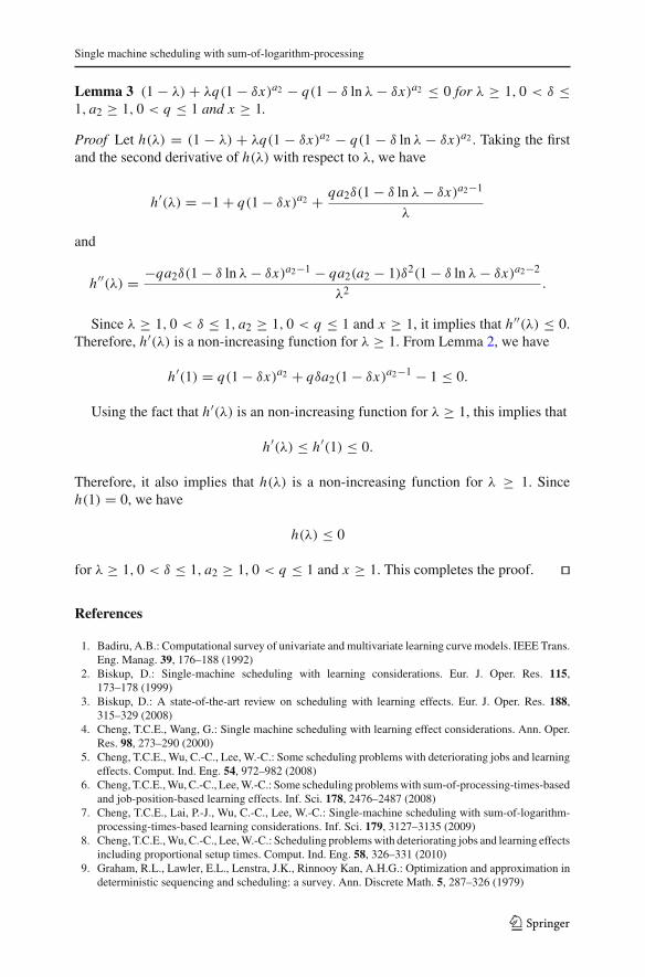
Lemma 3 (1 − λ) + λq(1 − δx)a2 − q(1 − δ ln λ − δx)a2 ≤ 0 for λ ≥ 1, 0 < δ ≤1, a2 ≥ 1, 0 < q ≤ 1 and x ≥ 1.
Proof Let h(λ) = (1 − λ) + λq(1 − δx)a2 − q(1 − δ ln λ − δx)a2 . Taking the firstand the second derivative of h(λ) with respect to λ, we have
h′(λ) = −1 + q(1 − δx)a2 + qa2δ(1 − δ ln λ − δx)a2−1
λ
and
h′′(λ) = −qa2δ(1 − δ ln λ − δx)a2−1 − qa2(a2 − 1)δ2(1 − δ ln λ − δx)a2−2
λ2 .
Since λ ≥ 1, 0 < δ ≤ 1, a2 ≥ 1, 0 < q ≤ 1 and x ≥ 1, it implies that h′′(λ) ≤ 0.Therefore, h′(λ) is a non-increasing function for λ ≥ 1. From Lemma 2, we have
h′(1) = q(1 − δx)a2 + qδa2(1 − δx)a2−1 − 1 ≤ 0.
Using the fact that h′(λ) is an non-increasing function for λ ≥ 1, this implies that
h′(λ) ≤ h′(1) ≤ 0.
Therefore, it also implies that h(λ) is a non-increasing function for λ ≥ 1. Sinceh(1) = 0, we have
h(λ) ≤ 0
for λ ≥ 1, 0 < δ ≤ 1, a2 ≥ 1, 0 < q ≤ 1 and x ≥ 1. This completes the proof. ��
References
1. Badiru, A.B.: Computational survey of univariate and multivariate learning curve models. IEEE Trans.Eng. Manag. 39, 176–188 (1992)
2. Biskup, D.: Single-machine scheduling with learning considerations. Eur. J. Oper. Res. 115,173–178 (1999)
3. Biskup, D.: A state-of-the-art review on scheduling with learning effects. Eur. J. Oper. Res. 188,315–329 (2008)
4. Cheng, T.C.E., Wang, G.: Single machine scheduling with learning effect considerations. Ann. Oper.Res. 98, 273–290 (2000)
5. Cheng, T.C.E., Wu, C.-C., Lee, W.-C.: Some scheduling problems with deteriorating jobs and learningeffects. Comput. Ind. Eng. 54, 972–982 (2008)
6. Cheng, T.C.E., Wu, C.-C., Lee, W.-C.: Some scheduling problems with sum-of-processing-times-basedand job-position-based learning effects. Inf. Sci. 178, 2476–2487 (2008)
7. Cheng, T.C.E., Lai, P.-J., Wu, C.-C., Lee, W.-C.: Single-machine scheduling with sum-of-logarithm-processing-times-based learning considerations. Inf. Sci. 179, 3127–3135 (2009)
8. Cheng, T.C.E., Wu, C.-C., Lee, W.-C.: Scheduling problems with deteriorating jobs and learning effectsincluding proportional setup times. Comput. Ind. Eng. 58, 326–331 (2010)
9. Graham, R.L., Lawler, E.L., Lenstra, J.K., Rinnooy Kan, A.H.G.: Optimization and approximation indeterministic sequencing and scheduling: a survey. Ann. Discrete Math. 5, 287–326 (1979)
123
J.-B. Wang, J.-J. Wang
10. Huang, X., Wang, J.-B., Wang, L.-Y., Gao, W.-J., Wang, X.-R.: Single machine scheduling with time-dependent deterioration and exponential learning effect. Comput. Ind. Eng. 58, 58–63 (2010)
11. Huang, X., Wang, M.-Z., Wang, J.-B.: Single machine group scheduling with both learning effects anddeteriorating jobs. Comput. Ind. Eng. 60, 750–754 (2011)
12. Lee, W.-C., Wu, C.-C.: Some single-machine and m-machine flowshop scheduling problems withlearning considerations. Inf. Sci. 179, 3885–3892 (2009)
13. Lee, W.-C., Wu, C.-C.: A note on single-machine group scheduling problems with position-basedlearning effect. Appl. Math. Model. 33, 2159–2163 (2009)
14. Mosheiov, G.: Minimizing total absolute deviation of job completion times: extensions to position-dependent processing times and parallel identical machines. J. Oper. Res. Soc. 59, 1422–1424 (2008)
15. Pinedo, M.: Scheduling: theory, algorithms, and systems. Prentice-Hall, Upper Saddle River (2002)16. Townsend, W.: The single machine problem with quadratic penalty function of completion times:
a branch-and-bound solution. Manag. Sci. 24, 530–534 (1978)17. Wang, J.-B.: Single-machine scheduling with past-sequence-dependent setup times and time-dependent
learning effect. Comput. Ind. Eng. 55, 584–591 (2008)18. Wang, J.-B.: Single-machine scheduling with a sum-of-actual-processing-time based learning effect.
J. Oper. Res. Soc. 61, 172–177 (2010)19. Wang, J.-B., Ng, C.T., Cheng, T.C.E., Liu, L.L.: Single-machine scheduling with a time-dependent
learning effect. Int. J. Prod. Econ. 111, 802–811 (2008)20. Wang, J.-B., Wang, D., Wang, L.-Y., Lin, L., Yin, N., Wang, W.-W.: Single machine scheduling with
exponential time-dependent learning effect and past-sequence-dependent setup times. Comput. Math.Appl. 57, 9–16 (2009)
21. Wang, J.-B., Wang, M.-Z.: Single machine multiple common due dates scheduling with generaljob-dependent learning curves. Comput. Math. Appl. 60, 2998–3002 (2010)
22. Wang, J.-B., Wang, M.-Z.: A revision of machine scheduling problems with a general learning effect.Math. Comput. Model. 53, 330–336 (2011)
23. Wang, J.-B., Li, J.-X.: Single machine past-sequence-dependent setup times scheduling with generalposition-dependent and time-dependent learning effects. Appl. Math. Model. 35, 1388–1395 (2011)
24. Wright, T.P.: Factors affecting the cost of airplanes. J. Aeronaut. Sci. 3, 122–128 (1936)25. Wu, C.C., Lee, W.C.: Single-machine and flowshop scheduling with a general learning effect
model. Comput. Ind. Eng. 56, 1553–1558 (2009)26. Yang, D.-L., Kuo, W.-H.: Single-machine scheduling with both deterioration and learning effects.
Ann. Oper. Res. 172, 315–327 (2009)27. Yang, D.-L., Kuo, W.-H.: Some scheduling problems with deteriorating jobs and learning effects.
Comput. Ind. Eng. 58, 25–28 (2010)28. Yin, Y., Xu, D., Sun, K., Li, H.: Some scheduling problems with general position-dependent and
time-dependent learning effects. Inf. Sci. 179, 2416–2425 (2009)29. Zhang, X., Yan, G., Zhang, F., Tang, G.: Machine scheduling algorithm with a new learning effect.
J. Syst. Sci. Math. Sci. 30, 1359–1367 (2010, in Chinese)
123