Embed Size (px)
Citation preview

arX
iv:1
610.
0665
6v2
[sta
t.ML]
26
Oct
201
6
Single Pass PCA of Matrix Products
Shanshan WuThe University of Texas at [email protected]
Srinadh BhojanapalliToyota Technological Institute at Chicago
Sujay SanghaviThe University of Texas at [email protected]
Alexandros G. DimakisThe University of Texas at Austin
October 27, 2016
Abstract
In this paper we present a new algorithm for computing a low rank approximation of the productATB by taking only a single pass of the two matricesA andB. The straightforward way to do this is to(a) first sketchA andB individually, and then (b) find the top components using PCA on the sketch. Ouralgorithm in contrast retains additional summary information aboutA,B (e.g. row and column normsetc.) and uses this additional information to obtain an improved approximation from the sketches. Ourmain analytical result establishes a comparable spectral norm guarantee to existing two-pass methods; inaddition we also provide results from an Apache Spark implementation that shows better computationaland statistical performance on real-world and synthetic evaluation datasets.
1 Introduction
Given two large matricesA andB we study the problem of finding a low rank approximation of theirproductATB, using only one pass over the matrix elements. This problem has many applications in machinelearning and statistics. For example, ifA = B, then this general problem reduces to Principal ComponentAnalysis (PCA). Another example is a low rank approximationof a co-occurrence matrix from large logs,e.g.,A may be a user-by-query matrix andB may be a user-by-ad matrix, soATB computes the jointcounts for each query-ad pair. The matricesA andB can also be two large bag-of-word matrices. For thiscase, each entry ofATB is the number of times a pair of words co-occurred together. As a fourth example,ATB can be a cross-covariance matrix between two sets of variables, e.g.,A andB may be genotype andphenotype data collected on the same set of observations. A low rank approximation of the product matrixis useful for Canonical Correlation Analysis (CCA) [8]. Forall these examples,ATB captures pairwisevariable interactions and a low rank approximation is a way to efficiently represent the significant pairwiseinteractions in sub-quadratic space.
Let A andB be matrices of sized × n (d ≫ n) assumed too large to fit in main memory. To obtain arank-r approximation ofATB, a naive way is to computeATB first, and then perform truncated singularvalue decomposition (SVD) ofATB. This algorithm needsO(n2d) time andO(n2) memory to computethe product, followed by an SVD of then×n matrix. An alternative option is to directly run power methodonATB without explicitly computing the product. Such an algorithm will need to access the data matricesA andB multiple times and the disk IO overhead for loading the matrices to memory multiple times will bethe major performance bottleneck.
1
For this reason, a number of recent papers introduce randomized algorithms that require only a fewpasses over the data, approximately linear memory, and alsoprovide spectral norm guarantees. The key stepin these algorithms is to compute a smaller representation of data. This can be achieved by two differentmethods: (1) dimensionality reduction, i.e., matrix sketching [29, 11, 26, 12]; (2) random sampling [14, 3].The recent results of Cohen et al. [12] provide the strongestspectral norm guarantee of the former. Theyshow that a sketch size ofO(r/ǫ2) suffices for the sketched matricesAT B to achieve a spectral error ofǫ,wherer is the maximum stable rank ofA andB. Note thatAT B is not the desired rank-r approximationof ATB. On the other hand, [3] is a recent sampling method with very good performance guarantees.The authors consider entrywise sampling based on column norms, followed by a matrix completion stepto compute low rank approximations. There is also a lot of interesting work on streaming PCA, but nonecan be directly applied to the general case whenA is different fromB (see Figure 4(c)). Please refer toAppendix D for more discussions on related work.
Despite the significant volume of prior work, there is no method that computes a rank-r approximationof ATB when the entries ofA andB are streaming in a single pass1. Bhojanapalli et al. [3] consider atwo-pass algorithm which computes column norms in the first pass and uses them to sample in a secondpass over the matrix elements. In this paper, we combine ideas from the sketching and sampling literatureto obtain the first algorithm that requires only a single passover the data.
Contributions:
• We propose a one-pass algorithm SMP-PCA (which stands for Streaming Matrix Product PCA) thatcomputes a rank-r approximation ofATB in time O((nnz(A) + nnz(B))ρ
2r3rη2
+ nr6ρ4r3
η4). Here
nnz(·) is the number of non-zero entries,ρ is the condition number,r is the maximum stable rank, andη measures the spectral norm error. Existing two-pass algorithms such as [3] typically have longerruntime than our algorithm (see Figure 3(a)). We also compare our algorithm with the simple idea thatfirst sketchesA andB separately and then performs SVD on the product of their sketches. We showthat our algorithmalwaysachieves better accuracy and can perform arbitrarily better if the columnvectors ofA andB come from a cone (see Figures 2, 4(b), 3(b)).
• The central idea of our algorithm is a novelrescaled JL embeddingthat combines information frommatrix sketches and vector norms. This allows us to get better estimates of dot products of highdimensional vectors compared to previous sketching approaches. We explain the benefit compared toa naive JL embedding in Figure 2 and the related discussion; we believe it may be of more generalinterest beyond low rank matrix approximations.
• We prove that our algorithm recovers a low rank approximation of ATB up to an error that dependson ‖ATB − (ATB)r‖ and ‖ATB‖, decaying with increasing sketch size and number of samples(Theorem 3.1). The first term is a consequence of low rank approximation and vanishes ifATB isexactly rank-r. The second term results from matrix sketching and subsampling; the bounds havesimilar dependencies as in [12].
• We implement SMP-PCA in Apache Spark and perform several distributed experiments on syntheticand real datasets. Our distributed implementation uses several design innovations described in Sec-tion 4 and Appendix C.5 and it is the only Spark implementation that we are aware of that can handlematrices that are large in both dimensions. Our experimentsshow that we improve by approximatelya factor of2× in running time compared to the previous state of the art and scale gracefully as thecluster size increases. The source code is available online[36].
1One straightforward idea is to sketch each matrix individually and perform SVD on the product of the sketches. We compareagainst that scheme and show that we can perform arbitrarilybetter using our rescaled JL embedding.
2

• In addition to better performance, our algorithm offers another advantage: It is possible to computelow-rank approximations toATB even when the entries of the two matrices arrive in some arbitraryorder (as would be the case in streaming logs). We can therefore discover significant correlations evenwhen the original datasets cannot be stored, for example dueto storage or privacy limitations.
2 Problem setting and algorithms
Consider the following problem: given two matricesA ∈ Rd×n1 andB ∈ Rd×n2 that are stored in disk,find a rank-r approximation of their productATB. In particular, we are interested in the setting whereboth A, B andATB are too large to fit into memory. This is common for modern large scale machinelearning applications. For this setting, we develop a single-pass algorithm SMP-PCA that computes therank-r approximation without explicitly forming the entire matrix ATB.
Notations. Throughout the paper, we useA(i, j) or Aij to denote(i, j) entry for any matrixA. LetAi andAj be thei-th column vector andj-th row vector. We use‖A‖F for Frobenius norm, and‖A‖ forspectral (or operator) norm. The optimal rank-r approximation of matrixA is Ar, which can be found bySVD. Given a setΩ ⊂ [n1]× [n2] and a matrixA ∈ Rn1×n2, we definePΩ(A) ∈ Rn1×n2 as the projectionof A onΩ, i.e.,PΩ(A)(i, j) = A(i, j) if (i, j) ∈ Ω and 0 otherwise.
2.1 SMP-PCA
Our algorithm SMP-PCA (Streaming Matrix Product PCA) takesfour parameters as input: the desired rankr, number of samplesm, sketch sizek, and the number of iterationsT . Performance guarantee involvingthese parameters is provided in Theorem 3.1. As illustratedin Figure 1, our algorithm has three main steps:1) compute sketches and side information in one pass overA andB; 2) given partial information ofA andB, estimateimportantentries ofATB; 3) compute low rank approximation given estimates of a few entriesof ATB. Now we explain each step in detail.
Figure 1: An overview of our algorithm. A single pass is performed over the data to produce the sketchedmatricesA, B and the column norms‖Ai‖, ‖Bj‖, for all (i, j) ∈ [n1] × [n2]. We then compute thesampled matrixPΩ(M) through a biased sampling process, wherePΩ(M) = M(i, j) if (i, j) ∈ Ω andzero otherwise. HereΩ represents the set of sampled entries. We defineM as an estimator forATB, and
compute its entry asM (i, j) = ‖Ai‖ · ‖Bj‖ · ATiBj
‖Ai‖·‖Bj‖. Performing matrix completion onPΩ(M ) gives the
desired rank-r approximation.
Step 1: Compute sketches and side information in one pass over A and B. In this step we computesketchesA := ΠA andB := ΠB, whereΠ ∈ Rk×d is a random matrix with entries being i.i.d.N (0, 1/k)
3
Algorithm 1 SMP-PCA: Streaming Matrix Product PCA
1: Input: A ∈ Rd×n1 , B ∈ Rd×n2, desired rank:r, sketch size:k, number of samples:m, number ofiterations:T
2: Construct a random matrixΠ ∈ Rk×d, whereΠ(i, j) ∼ N (0, 1/k), ∀(i, j) ∈ [k]× [d]. Perform a singlepass overA andB to obtain:A = ΠA, B = ΠB, and‖Ai‖, ‖Bj‖, ∀(i, j) ∈ [n1]× [n2].
3: Sample each entry(i, j) ∈ [n1] × [n2] independently with probabilityqij = min1, qij, whereqij isdefined in Eq.(1); maintain a setΩ ⊂ [n1]× [n2] which stores all the sampled pairs(i, j).
4: DefineM ∈ Rn1×n2 , whereM(i, j) is given in Eq. (2). CalculatePΩ(M ) ∈ Rn1×n2 , wherePΩ(M ) =
M(i, j) if (i, j) ∈ Ω and zero otherwise.5: Run WAltMin(PΩ(M ), Ω, r, q, T ), see Appendix A for more details.6: Output: U ∈ Rn1×r andV ∈ Rn2×r.
random variables. It is known thatΠ satisfies an ”oblivious Johnson-Lindenstrauss (JL) guarantee” [29][34]and it helps preserving the top row spaces ofA andB [11]. Note that any sketching matrixΠ that is anoblivious subspace embedding can be considered here, e.g.,sparse JL transform and randomized Hadamardtransform (see [12] for more discussion).
BesidesA andB, we also compute theL2 norms for all column vectors, i.e.,‖Ai‖ and‖Bj‖, for all(i, j) ∈ [n1] × [n2]. We use this additional information to design better estimates ofATB in the next step,and also to determineimportantentries ofAT B to sample. Note that this is the only step that needs onepass over data.
Step 2: Estimate important entries ofATB by rescaled JL embedding.In this step we use partialinformation obtained from the previous step to compute a fewimportant entries ofAT B. We first determinewhat entries ofAT B to sample, and then propose a novel rescaled JL embedding forestimating those entries.
We sample entry(i, j) of ATB independently with probabilityqij = min1, qij, where
qij = m · ( ‖Ai‖22n2‖A‖2F
+‖Bj‖2
2n1‖B‖2F). (1)
Let Ω ⊂ [n1] × [n2] be the set of sampled entries(i, j). SinceE(∑
i,j qij) = m, the expected numberof sampled entries is roughlym. The special form ofqij ensures that we can drawm samples inO(n1 +m log(n2)) time; we show how to do this in Appendix C.5.
Note thatqij intuitively captures important entries ofATB by giving higher weight to heavy rows andcolumns. We show in Section 3 that this sampling actually generates good approximation to the matrixATB.
The biased sampling distribution of Eq. (1) is first proposedby Bhojanapalli et al. [3]. However,their algorithm [3] needs a second pass to compute the sampled entries, while we propose a novel way ofestimating dot products, using information obtained in thefirst step.
DefineM ∈ Rn1×n2 as
M(i, j) = ‖Ai‖ · ‖Bj‖ ·AT
i Bj
‖Ai‖ · ‖Bj‖. (2)
Note that we will not compute and storeM , instead, we only calculateM(i, j) for (i, j) ∈ Ω. This matrixis denoted asPΩ(M), wherePΩ(M )(i, j) = M(i, j) if (i, j) ∈ Ω and 0 otherwise.
We now explain the intuition of Eq. (2), and whyM is a better estimator thanAT B. To estimate the(i, j) entry ofATB, a straightforward way is to useAT
i Bj = ‖Ai‖ · ‖Bj‖ · cos θij, whereθij is the anglebetween vectorsAi andBj. Since we already know the actual column norms, a potentially better estimator
4
-1 -0.5 0 0.5 1
True dot product
-2
-1
0
1
2E
stim
ated
dot
pro
duct
JL embeddingRescaled JL embedding
(a) (b)
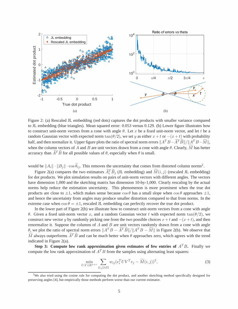
Figure 2: (a) Rescaled JL embedding (red dots) captures the dot products with smaller variance comparedto JL embedding (blue triangles). Mean squared error: 0.053versus 0.129. (b) Lower figure illustrates howto construct unit-norm vectors from a cone with angleθ. Let x be a fixed unit-norm vector, and lett be arandom Gaussian vector with expected normtan(θ/2), we sety as eitherx+ t or−(x+ t) with probabilityhalf, and then normalize it. Upper figure plots the ratio of spectral norm errors‖ATB−AT B‖/‖ATB−M‖,when the column vectors ofA andB are unit vectors drawn from a cone with angleθ. Clearly,M has betteraccuracy thanAT B for all possible values ofθ, especially whenθ is small.
would be‖Ai‖ · ‖Bj‖ · cos θij . This removes the uncertainty that comes from distorted column norms2.Figure 2(a) compares the two estimatorsAT
i Bj (JL embedding) andM(i, j) (rescaled JL embedding)for dot products. We plot simulation results on pairs of unit-norm vectors with different angles. The vectorshave dimension 1,000 and the sketching matrix has dimension10-by-1,000. Clearly rescaling by the actualnorms help reduce the estimation uncertainty. This phenomenon is more prominent when the true dotproducts are close to±1, which makes sense becausecos θ has a small slope whencos θ approaches±1,and hence the uncertainty from angles may produce smaller distortion compared to that from norms. In theextreme case whencos θ = ±1, rescaled JL embedding can perfectly recover the true dot product.
In the lower part of Figure 2(b) we illustrate how to construct unit-norm vectors from a cone with angleθ. Given a fixed unit-norm vectorx, and a random Gaussian vectort with expected normtan(θ/2), weconstruct new vectory by randomly picking one from the two possible choicesx+ t and−(x+ t), and thenrenormalize it. Suppose the columns ofA andB are unit vectors randomly drawn from a cone with angleθ, we plot the ratio of spectral norm errors‖ATB − AT B‖/‖ATB − M‖ in Figure 2(b). We observe thatM always outperformsAT B and can be much better whenθ approaches zero, which agrees with the trendindicated in Figure 2(a).
Step 3: Compute low rank approximation given estimates of few entries of ATB. Finally wecompute the low rank approximation ofATB from the samples using alternating least squares:
minU,V ∈Rn×r
∑
(i,j)∈Ω
wij(eTi UV T ej − M(i, j))2, (3)
2We also tried using the cosine rule for computing the dot product, and another sketching method specifically designed forpreserving angles [4], but empirically those methods perform worse than our current estimator.
5
wherewij = 1/qij denotes the weights, andei, ej are standard base vectors. This is a popular technique forlow rank recovery and matrix completion (see [3] and the references therein). AfterT iterations, we will geta rank-r approximation ofM presented in the convenient factored form. This subroutineis quite standard,so we defer the details to Appendix A.
3 Analysis
Now we present the main theoretical result. Theorem 3.1 characterizes the interaction between the sketch
sizek, the sampling complexitym, the number of iterationsT , and the spectral error‖(ATB)r − ATBr‖,
whereATBr is the output of SMP-PCA, and(ATB)r is the optimal rank-r approximation ofATB. Notethat the following theorem assumes thatA andB have the same size. For the general case ofn1 6= n2,Theorem 3.1 is still valid by settingn = maxn1, n2.
Theorem 3.1. Given matricesA ∈ Rd×n andB ∈ Rd×n, let (ATB)r be the optimal rank-r approximation
of ATB. Definer = max‖A‖2F
‖A‖2 ,‖B‖2
F
‖B‖2 as the maximum stable rank, andρ =σ∗
1
σ∗
ras the condition number
of (ATB)r, whereσ∗i is thei-th singular values ofATB.
Let ATBr be the output of AlgorithmSMP-PCA. If the input parametersk, m, andT satisfy
k ≥ C1‖A‖2‖B‖2ρ2r3‖ATB‖2F
· maxr, 2 log(n)+ log (3/γ)
η2, (4)
m ≥ C2r2
γ·(‖A‖2F + ‖B‖2F
‖ATB‖F
)2
· nr3ρ2 log(n)T 2
η2, (5)
T ≥ log(‖A‖F + ‖B‖F
ζ), (6)
whereC1 andC2 are some global constants independent ofA andB. Then with probability at least1− γ,we have
‖(ATB)r − ATBr‖ ≤ η‖ATB − (ATB)r‖F + ζ + ησ∗r . (7)
Remark 1. Compared to the two-pass algorithm proposed by [3], we notice that Eq. (7) contains anadditional error termησ∗
r . This extra term captures the cost incurred when we are approximating entries ofATB by Eq. (2) instead of using the actual values. The exact tradeoff betweenη andk is given by Eq. (4).On one hand, we want to have a smallk so that the sketched matrices can fit into memory. On the otherhand, the parameterk controls how much information is lost during sketching, anda largerk gives a moreaccurate estimation of the inner products.
Remark 2. The dependence on‖A‖2
F+‖B‖2
F
‖ATB‖Fcaptures one difficult situation for our algorithm. If
‖ATB‖F is much smaller than‖A‖F or ‖B‖F , which could happen, e.g., when many column vectorsof A are orthogonal to those ofB, then SMP-PCA requires many samples to work. This is reasonable.Imagine thatATB is close to an identity matrix, then it may be hard to tell it from an all-zero matrix withoutenough samples. Nevertheless, removing this dependence isan interesting direction for future research.
Remark 3. For the special case ofA = B, SMP-PCA computes a rank-r approximation of ma-trix ATA in a single pass. Theorem 3.1 provides an error bound in spectral norm for the residual matrix
(ATA)r − ATAr. Most results in the online PCA literature use Frobenius norm as performance measure.Recently, [22] provides an online PCA algorithm with spectral norm guarantee. They achieves a spectralnorm bound ofǫσ∗
1+σ∗r+1, which is stronger than ours. However, their algorithm requires a target dimension
6
of O(r log n/ǫ2), i.e., the output is a matrix of sizen-by-O(r log n/ǫ2), while the output of SMP-PCA issimplyn-by-r.
Remark 4. We defer our proofs to Appendix C. The proof proceeds in threesteps. In Appendix C.2, weshow that the sampled matrix provides a good approximation of the actual matrixATB. In Appendix C.3,we show that there is a geometric decrease in the distance between the computed subspacesU , V and theoptimal onesU∗, V ∗ at each iteration of WAltMin algorithm. The spectral norm bound in Theorem 3.1 isthen proved using results from the previous two steps.
Computation Complexity. We now analyze the computation complexity of SMP-PCA. In Step 1, wecompute the sketched matrices ofA andB, which requiresO(nnz(A)k + nnz(B)k) flops. Here nnz(·)denotes the number of non-zero entries. The main job of Step 2is to sample a setΩ and calculate thecorresponding inner products, which takesO(m log(n) +mk) flops. Here we definen asmaxn1, n2 forsimplicity. According to Eq. (4), we havelog(n) = O(k), so Step 2 takesO(mk) flops. In Step 3, we runalternating least squares on the sampled matrix, which can be completed inO((mr2 + nr3)T ) flops. SinceEq. (5) indicatesnr = O(m), the computation complexity of Step 3 isO(mr2T ). Therefore, SMP-PCAhas a total computation complexityO(nnz(A)k + nnz(B)k +mk +mr2T ).
4 Numerical Experiments
Spark implementation. We implement our SMP-PCA in Apache Spark 1.6.2 [37]. For the purpose ofcomparison, we also implement a two-pass algorithm LELA [3]in Spark3. The matricesA andB arestored as a resilient distributed dataset (RDD) in disk (by setting itsStorageLevel asDISK_ONLY). Weimplement the two passes of LELA using thetreeAggregatemethod. For SMP-PCA, we choose thesubsampled randomized Hadamard transform (SRHT) [32] as the sketching matrix4. The biased samplingprocedure is performed using binary search (see Appendix C.5 for how to samplem elements inO(m log n)time). After obtaining the sampled matrix, we runALS (alternating least squares) to get the desired low-rankmatrices. More details can be found in [36].
Description of datasets.We test our algorithm on synthetic datasets and three real datasets: SIFT10K [20],NIPS-BW [23], and URL-reputation [24]. For synthetic data,we generate matricesA andB asGD, whereG has entries independently drawn from standard Gaussian distribution, andD is a diagonal matrix withDii = 1/i. SIFT10K is a dataset of 10,000 images. Each image is represented by 128 features. We setA asthe image-by-feature matrix. The task here is to compute a low rank approximation ofATA, which is a stan-dard PCA task. The NIPS-BW dataset contains bag-of-words features extracted from 1,500 NIPS papers.We divide the papers into two subsets, and letA andB be the corresponding word-by-paper matrices, soATB computes the counts of co-occurred words between two sets ofpapers. The original URL-reputationdataset has 2.4 million URLs. Each URL is represented by 3.2 million features, and is indicated as ma-licious or benign. This dataset has been used previously forCCA [25]. Here we extract two subsets offeatures, and letA andB be the corresponding URL-by-feature matrices. The goal is to compute a low rankapproximation ofATB, the cross-covariance matrix between two subsets of features.
Sample complexity.In Figure 4(a) we present simulation results on a small synthetic data withn = d =5, 000 andr = 5. We observe that a phase transition occurs when the sample complexitym = Θ(nr log n).This agrees with the experimental results shown in previouspapers, see, e.g., [9, 3]. For the rest experimentspresented in this section, unless otherwise specified, we set r = 5, T = 10, and sampling complexitym as4nr log n.
3To our best knowledge, this the first distributed implementation of LELA.4Compared to Gaussian sketch, SRHT reduces the runtime fromO(ndk) to O(nd log d) and space cost fromO(dk) to O(d),
while maintains the same quality of the output.
7

2 5 100
1000
2000
3000
Runtime (sec) vs Cluster size
LELASMC-PCA
(a)
1000 2000
Sketch size (k)
0.05
0.1
0.15
0.2
Spe
ctra
l nor
m e
rror
SVD(ATB)
SMP-PCALELAOptimal
1000 2000
Sketch size (k)
0.05
0.1
0.15
0.2
0.25
0.3 SVD(ATB)
SMP-PCALELAOptimal
(b)
Figure 3: (a) Spark-1.6.2 running time on a 150GB dataset. All nodes are m.2xlarge EC2 instances. See [36]for more details. (b) Spectral norm error achieved by three algorithms over two datasets: SIFT10K (left)and NIPS-BW (right). We observe that SMP-PCA outperforms SVD(AT B) by a factor of 1.8 for SIFT10Kand 1.1 for NIPS-BW. Besides, the error of SMP-PCA keeps decreasing as the sketch sizek grows.
Table 1: A comparison of spectral norm error over three datasets
Dataset d n Algorithm Sketch sizek Error
Synthetic 100,000 100,000Optimal - 0.0271LELA - 0.0274
SMP-PCA 2,000 0.0280
URL-malicious
792,145 10,000Optimal - 0.0163LELA - 0.0182
SMP-PCA 2,000 0.0188
URL-benign
1,603,985 10,000Optimal - 0.0103LELA - 0.0105
SMP-PCA 2,000 0.0117
Comparison of SMP-PCA and LELA. We now compare the statistical performance of SMP-PCAand LELA [3] on three real datasets and one synthetic dataset. As shown in Figure 3(b) and Table 1, LELAalways achieves a smaller spectral norm error than SMP-PCA,which makes sense because LELA takestwo passes and hence has more chances exploring the data. Besides, we observe that as the sketch sizeincreases, the error of SMP-PCA keeps decreasing and gets closer to that of LELA.
In Figure 3(a) we compare the runtime of SMP-PCA and LELA using a 150GB synthetic dataset onm3.2xlarge Amazon EC2 instances5. The matricesA andB have dimensionn = d = 100, 000. The sketchdimension is set ask = 2, 000. We observe that the speedup achieved by SMP-PCA is more prominent forsmall clusters (e.g., 56 mins versus 34 mins on a cluster of size two). This is possibly due to the increasingspark overheads at larger clusters, see [17] for more related discussion.
Comparison of SMP-PCA and SVD(AT B). In Figure 4(b) we repeat the experiment in Section 2 bygenerating column vectors ofA andB from a cone with angleθ. Here SVD(AT B) refers to computing
5Each machine has 8 cores, 30GB memory, and 2×80GB SSD.
8
1 2 3 4# Samples / nrlogn
0.2
0.3
0.4
0.5S
pect
ral n
orm
err
ork = 400
k = 800
(a)
0 π/4 π/2 3π/4 π
100
105Ratio of errors vs theta
(b)
200 400 600 800 1000Sketch size (k)
0.2
0.4
0.6
0.8
1
Spe
ctra
l nor
m e
rror
AT
rBr
SMP-PCA
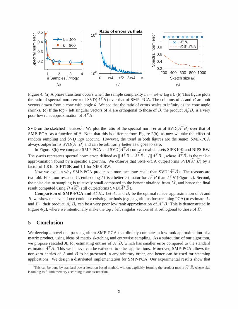
(c)
Figure 4: (a) A phase transition occurs when the sample complexity m = Θ(nr log n). (b) This figure plotsthe ratio of spectral norm error of SVD(AT B) over that of SMP-PCA. The columns ofA andB are unitvectors drawn from a cone with angleθ. We see that the ratio of errors scales to infinity as the cone angleshrinks. (c) If the topr left singular vectors ofA are orthogonal to those ofB, the productAT
r Br is a verypoor low rank approximation ofATB.
SVD on the sketched matrices6. We plot the ratio of the spectral norm error of SVD(AT B) over that ofSMP-PCA, as a function ofθ. Note that this is different from Figure 2(b), as now we take the effect ofrandom sampling and SVD into account. However, the trend in both figures are the same: SMP-PCAalways outperforms SVD(AT B) and can be arbitrarily better asθ goes to zero.
In Figure 3(b) we compare SMP-PCA and SVD(AT B) on two real datasets SIFK10K and NIPS-BW.
The y-axis represents spectral norm error, defined as||ATB − ATBr||/||ATB||, whereATBr is the rank-rapproximation found by a specific algorithm. We observe thatSMP-PCA outperforms SVD(AT B) by afactor of 1.8 for SIFT10K and 1.1 for NIPS-BW.
Now we explain why SMP-PCA produces a more accurate result than SVD(AT B). The reasons aretwofold. First, our rescaled JL embeddingM is a better estimator forATB thanAT B (Figure 2). Second,the noise due to sampling is relatively small compared to thebenefit obtained fromM , and hence the finalresult computed usingPΩ(M ) still outperforms SVD(AT B).
Comparison of SMP-PCA andATr Br. Let Ar andBr be the optimal rank-r approximation ofA and
B, we show that even if one could use existing methods (e.g., algorithms for streaming PCA) to estimateAr
andBr, their productATr Br can be a very poor low rank approximation ofATB. This is demonstrated in
Figure 4(c), where we intentionally make the topr left singular vectors ofA orthogonal to those ofB.
5 Conclusion
We develop a novel one-pass algorithm SMP-PCA that directlycomputes a low rank approximation of amatrix product, using ideas of matrix sketching and entrywise sampling. As a subroutine of our algorithm,we propose rescaled JL for estimating entries ofATB, which has smaller error compared to the standardestimatorAT B. This we believe can be extended to other applications. Moreover, SMP-PCA allows thenon-zero entries ofA andB to be presented in any arbitrary order, and hence can be used for steamingapplications. We design a distributed implementation for SMP-PCA. Our experimental results show that
6This can be done by standard power iteration based method, without explicitly forming the product matrixATB, whose size
is too big to fit into memory according to our assumption.
9

SMP-PCA can perform arbitrarily better than SVD(AT B), and is significantly faster compared to algo-rithms that require two or more passes over the data.
AcknowledgementsWe thank the anonymous reviewers for their valuable comments. This research hasbeen supported by NSF Grants CCF 1344179, 1344364, 1407278,1422549, 1302435, 1564000, and AROYIP W911NF-14-1-0258.
10
References
[1] D. Achlioptas and F. McSherry. Fast computation of low rank matrix approximations. InProceedingsof the thirty-third annual ACM symposium on Theory of computing, pages 611–618. ACM, 2001.
[2] A. Balsubramani, S. Dasgupta, and Y. Freund. The fast convergence of incremental pca. InAdvancesin Neural Information Processing Systems, pages 3174–3182, 2013.
[3] S. Bhojanapalli, P. Jain, and S. Sanghavi. Tighter low-rank approximation via sampling the leveragedelement. InProceedings of the Twenty-Sixth Annual ACM-SIAM Symposiumon Discrete Algorithms(SODA), pages 902–920. SIAM, 2015.
[4] P. T. Boufounos. Angle-preserving quantized phase embeddings. InSPIE Optical Engineering+Applications. International Society for Optics and Photonics, 2013.
[5] C. Boutsidis, D. Garber, Z. Karnin, and E. Liberty. Online principal components analysis. InPro-ceedings of the Twenty-Sixth Annual ACM-SIAM Symposium on Discrete Algorithms, pages 887–901.SIAM, 2015.
[6] C. Boutsidis and A. Gittens. Improved matrix algorithmsvia the subsampled randomized hadamardtransform.SIAM Journal on Matrix Analysis and Applications, 34(3):1301–1340, 2013.
[7] E. J. Candes and B. Recht. Exact matrix completion via convex optimization.Foundations of Compu-tational mathematics, 9(6):717–772, 2009.
[8] X. Chen, H. Liu, and J. G. Carbonell. Structured sparse canonical correlation analysis. InInternationalConference on Artificial Intelligence and Statistics, pages 199–207, 2012.
[9] Y. Chen, S. Bhojanapalli, S. Sanghavi, and R. Ward. Completing any low-rank matrix, provably.arXivpreprint arXiv:1306.2979, 2013.
[10] K. L. Clarkson and D. P. Woodruff. Numerical linear algebra in the streaming model. InProceedingsof the forty-first annual ACM symposium on Theory of computing, pages 205–214. ACM, 2009.
[11] K. L. Clarkson and D. P. Woodruff. Low rank approximation and regression in input sparsity time. InProceedings of the 45th annual ACM symposium on Symposium ontheory of computing, pages 81–90.ACM, 2013.
[12] M. B. Cohen, J. Nelson, and D. P. Woodruff. Optimal approximate matrix product in terms of stablerank. arXiv preprint arXiv:1507.02268, 2015.
[13] A. Deshpande and S. Vempala. Adaptive sampling and fastlow-rank matrix approximation. InApprox-imation, Randomization, and Combinatorial Optimization.Algorithms and Techniques, pages 292–303. Springer, 2006.
[14] P. Drineas, R. Kannan, and M. W. Mahoney. Fast monte carlo algorithms for matrices ii: Computing alow-rank approximation to a matrix.SIAM Journal on Computing, 36(1):158–183, 2006.
[15] P. Drineas, M. W. Mahoney, and S. Muthukrishnan. Subspace sampling and relative-error matrixapproximation: Column-based methods. InApproximation, Randomization, and Combinatorial Opti-mization. Algorithms and Techniques, pages 316–326. Springer, 2006.
[16] A. Frieze, R. Kannan, and S. Vempala. Fast monte-carlo algorithms for finding low-rank approxima-tions. Journal of the ACM (JACM), 51(6):1025–1041, 2004.
11
[17] A. Gittens, A. Devarakonda, E. Racah, M. F. Ringenburg,L. Gerhardt, J. Kottalam, J. Liu, K. J.Maschhoff, S. Canon, J. Chhugani, P. Sharma, J. Yang, J. Demmel, J. Harrell, V. Krishnamurthy,M. W. Mahoney, and Prabhat. Matrix factorization at scale: acomparison of scientific data analyticsin spark and C+MPI using three case studies.arXiv preprint arXiv:1607.01335, 2016.
[18] N. Halko, P.-G. Martinsson, and J. A. Tropp. Finding structure with randomness: Probabilistic algo-rithms for constructing approximate matrix decompositions. SIAM review, 53(2):217–288, 2011.
[19] S. Har-Peled. Low rank matrix approximation in linear time. Manuscript. http://valis. cs. uiuc.edu/sariel/papers/05/lrank/lrank. pdf, 2006.
[20] H. Jegou, M. Douze, and C. Schmid. Product quantizationfor nearest neighbor search.Pattern Analysisand Machine Intelligence, IEEE Transactions on, 33(1):117–128, 2011.
[21] R. Kannan, S. S. Vempala, and D. P. Woodruff. Principal component analysis and higher correlationsfor distributed data. InProceedings of The 27th Conference on Learning Theory, pages 1040–1057,2014.
[22] Z. Karnin and E. Liberty. Online pca with spectral bounds. InProceedings of The 28th Conference onLearning Theory (COLT), volume 40, pages 1129–1140, 2015.
[23] M. Lichman. UCI machine learning repository. http://archive.ics.uci.edu/ml, 2013.
[24] J. Ma, L. K. Saul, S. Savage, and G. M. Voelker. Identifying suspicious urls: an application of large-scale online learning. InProceedings of the 26th annual international conference onmachine learning,pages 681–688. ACM, 2009.
[25] Z. Ma, Y. Lu, and D. Foster. Finding linear structure in large datasets with scalable canonical correla-tion analysis.arXiv preprint arXiv:1506.08170, 2015.
[26] A. Magen and A. Zouzias. Low rank matrix-valued chernoff bounds and approximate matrix multipli-cation. InProceedings of the twenty-second annual ACM-SIAM symposium on Discrete Algorithms,pages 1422–1436. SIAM, 2011.
[27] I. Mitliagkas, C. Caramanis, and P. Jain. Memory limited, streaming pca. InAdvances in NeuralInformation Processing Systems, pages 2886–2894, 2013.
[28] N. H. Nguyen, T. T. Do, and T. D. Tran. A fast and efficient algorithm for low-rank approximation ofa matrix. InProceedings of the 41st annual ACM symposium on Theory of computing, pages 215–224.ACM, 2009.
[29] T. Sarlos. Improved approximation algorithms for large matrices via random projections. InFounda-tions of Computer Science, 2006. FOCS’06. 47th Annual IEEE Symposium on, pages 143–152. IEEE,2006.
[30] O. Shamir. A stochastic pca and svd algorithm with an exponential convergence rate. InProceedingsof the 32nd International Conference on Machine Learning (ICML-15), pages 144–152, 2015.
[31] T. Tao. 254a, notes 3a: Eigenvalues and sums of hermitian matrices.Terence Tao’s blog, 2010.
[32] J. A. Tropp. Improved analysis of the subsampled randomized hadamard transform.Advances inAdaptive Data Analysis, pages 115–126, 2011.
12
[33] J. A. Tropp. User-friendly tail bounds for sums of random matrices.Foundations of ComputationalMathematics, 12(4):389–434, 2012.
[34] D. P. Woodruff. Sketching as a tool for numerical linearalgebra. arXiv preprint arXiv:1411.4357,2014.
[35] F. Woolfe, E. Liberty, V. Rokhlin, and M. Tygert. A fast randomized algorithm for the approximationof matrices.Applied and Computational Harmonic Analysis, 25(3):335–366, 2008.
[36] S. Wu, S. Bhojanapalli, S. Sanghavi, and A. Dimakis. Github repository for ”single-pass pca of matrixproducts”.https://github.com/wushanshan/MatrixProductPCA, 2016.
[37] M. Zaharia, M. Chowdhury, T. Das, A. Dave, J. Ma, M. McCauley, M. J. Franklin, S. Shenker, andI. Stoica. Resilient distributed datasets: A fault-tolerant abstraction for in-memory cluster computing.In Proceedings of the 9th USENIX conference on Networked Systems Design and Implementation,2012.
13
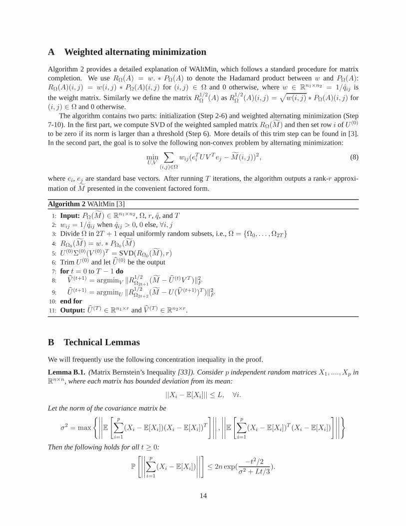
A Weighted alternating minimization
Algorithm 2 provides a detailed explanation of WAltMin, which follows a standard procedure for matrixcompletion. We useRΩ(A) = w. ∗ PΩ(A) to denote the Hadamard product betweenw andPΩ(A):RΩ(A)(i, j) = w(i, j) ∗ PΩ(A)(i, j) for (i, j) ∈ Ω and 0 otherwise, wherew ∈ Rn1×n2 = 1/qij is
the weight matrix. Similarly we define the matrixR1/2Ω (A) asR1/2
Ω (A)(i, j) =√
w(i, j) ∗ PΩ(A)(i, j) for(i, j) ∈ Ω and 0 otherwise.
The algorithm contains two parts: initialization (Step 2-6) and weighted alternating minimization (Step7-10). In the first part, we compute SVD of the weighted sampled matrixRΩ(M) and then set rowi of U (0)
to be zero if its norm is larger than a threshold (Step 6). Moredetails of this trim step can be found in [3].In the second part, the goal is to solve the following non-convex problem by alternating minimization:
minU,V
∑
(i,j)∈Ω
wij(eTi UV T ej − M(i, j))2, (8)
whereei, ej are standard base vectors. After runningT iterations, the algorithm outputs a rank-r approxi-mation ofM presented in the convenient factored form.
Algorithm 2 WAltMin [3]
1: Input: PΩ(M) ∈ Rn1×n2, Ω, r, q, andT2: wij = 1/qij whenqij > 0, 0 else,∀i, j3: DivideΩ in 2T + 1 equal uniformly random subsets, i.e.,Ω = Ω0, . . . ,Ω2T 4: RΩ0
(M ) = w. ∗ PΩ0(M)
5: U (0)Σ(0)(V (0))T = SVD(RΩ0(M ), r)
6: Trim U (0) and letU (0) be the output7: for t = 0 to T − 1 do8: V (t+1) = argminV ‖R1/2
Ω2t+1(M − U (t)V T )‖2F
9: U (t+1) = argminU ‖R1/2Ω2t+2
(M − U(V (t+1))T )‖2F10: end for11: Output: U (T ) ∈ Rn1×r andV (T ) ∈ Rn2×r.
B Technical Lemmas
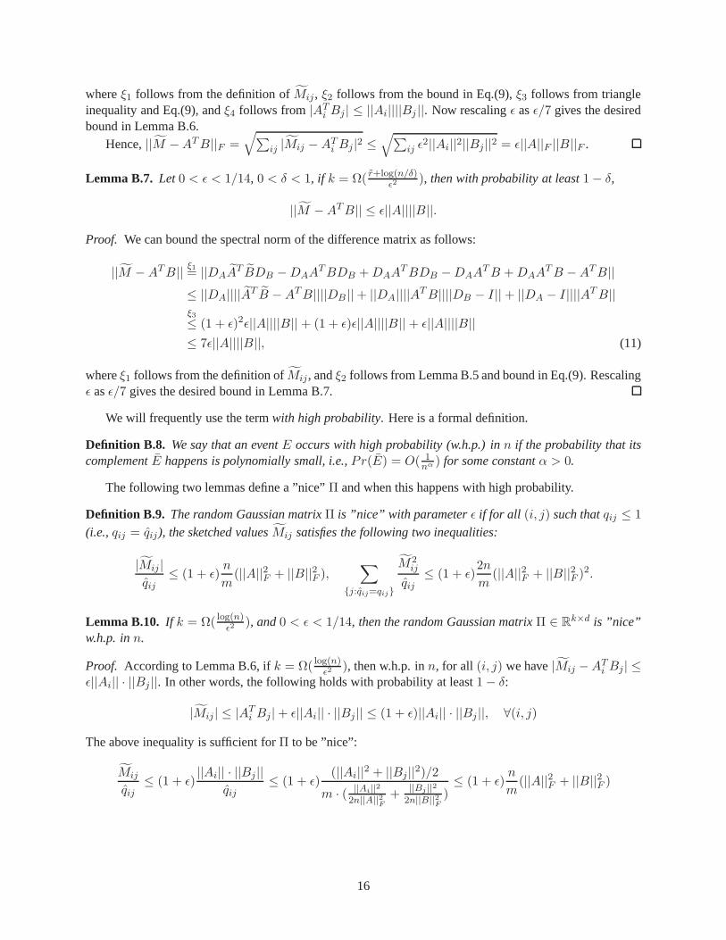
We will frequently use the following concentration inequality in the proof.
Lemma B.1. (Matrix Bernstein’s Inequality[33]). Considerp independent random matricesX1, ....,Xp inRn×n, where each matrix has bounded deviation from its mean:
||Xi − E[Xi]|| ≤ L, ∀i.Let the norm of the covariance matrix be
σ2 = max
∣∣∣∣∣
∣∣∣∣∣E[
p∑
i=1
(Xi − E[Xi])(Xi − E[Xi])T
]∣∣∣∣∣
∣∣∣∣∣ ,∣∣∣∣∣
∣∣∣∣∣E[
p∑
i=1
(Xi − E[Xi])T (Xi − E[Xi])
]∣∣∣∣∣
∣∣∣∣∣
Then the following holds for allt ≥ 0:
P
[∣∣∣∣∣
∣∣∣∣∣
p∑
i=1
(Xi − E[Xi])
∣∣∣∣∣
∣∣∣∣∣
]≤ 2n exp(
−t2/2
σ2 + Lt/3).
14

A formal definition of JL transform is given below [29][34].
Definition B.2. A random matrixΠ ∈ Rk×d forms a JL transform with parametersǫ, δ, f or JLT(ǫ, δ, f )for short, if with probability at least1− δ, for anyf -element subsetV ⊂ Rd, for all v, v′ ∈ V it holds that|〈Πv,Πv′〉 − 〈v, v′〉| ≤ ǫ||v|| · ||v′||.
The following lemma [34] characterizes the tradeoff between the reduced dimensionk and the errorlevel ǫ.
Lemma B.3. Let 0 < ǫ, δ < 1, andΠ ∈ Rk×d be a random matrix where the entriesΠ(i, j) are i.i.d.N (0, 1/k) random variables. Ifk = Ω(log(f/δ)ǫ−2), thenΠ is a JLT(ǫ, δ, f ).
We now present two lemmas that connectA ∈ Rk×n andB ∈ Rd×n with A ∈ Rd×n andB ∈ Rd×n.
Lemma B.4. Let0 < ǫ, δ < 1, if k = Ω( log(2n/δ)ǫ2
), then with probability at least1− δ,
(1− ǫ)||A||2F ≤ ||A||2F ≤ (1 + ǫ)||A||2F , (1− ǫ)||B||2F ≤ ||B||2F ≤ (1 + ǫ)||B||2F ,
||AT B −ATB||F ≤ ǫ||A||F ||B||F .Proof. This is again a standard result of JL transformation, e.g., see Definition 2.3 and Theorem 2.1 of [34]and Lemma 6 of [29] .
Lemma B.5. Let0 < ǫ, δ < 1, if k = Θ( r+log(1/δ)ǫ2 ), wherer = max ||A||2
F
||A||2 ,||B||2
F
||B||2 is the maximum stablerank, then with probability at least1− δ,
||AT B −ATB|| ≤ ǫ||A||||B||.
Proof. This follows from a recent paper [12].
Using the above two lemmas, we can prove the following two lemmas that relateM with ATB, for Mdefined in Algorithm 1. A more compact definition ofM is DAA
T BDB , whereDA andDB are diagonalmatrices with(DA)ii = ||Ai||/||Ai|| and(DB)jj = ||Bj ||/||Bj ||.
Lemma B.6. Let0 < ǫ < 1/14, 0 < δ < 1, if k = Ω( log(2n/δ)ǫ2 ), then with probability at least1− δ,
|Mij −ATi Bj | ≤ ǫ||Ai|| · ||Bj ||, ||M −ATB||F ≤ ǫ||A||F ||B||F .
Proof. Let 0 < ǫ < 1/2, 0 < δ < 1, according to the Definition B.2 and Lemma B.3, we have that ifk = Ω( log(2n/δ)
ǫ2), then with probability at least1− δ, and for alli, j
1− ǫ ≤ (DA)ii ≤ 1 + ǫ, 1− ǫ ≤ (DB)jj ≤ 1 + ǫ, |ATi Bj −AT
i Bj | ≤ ǫ||Ai||||Bj ||. (9)
We can now bound|Mij −ATi Bj| as
|Mij −ATi Bj |
ξ1= |AT
i Bj(DA)ii(DB)jj −ATi Bj|
ξ2≤ max|AT
i Bj(1 + ǫ)2 −ATi Bj |, |AT
i Bj(1− ǫ)2 −ATi Bj |
ξ3≤ max(1 + ǫ)2ǫ||Ai||||Bj ||+ ((1 + ǫ)2 − 1)|AT
i Bj |, (1− ǫ)2ǫ||Ai||||Bj ||+ (1− (1− ǫ)2)|ATi Bj |
ξ4≤ 7ǫ||Ai||||Bj ||, (10)
15
whereξ1 follows from the definition ofMij , ξ2 follows from the bound in Eq.(9),ξ3 follows from triangleinequality and Eq.(9), andξ4 follows from |AT
i Bj | ≤ ||Ai||||Bj ||. Now rescalingǫ asǫ/7 gives the desiredbound in Lemma B.6.
Hence,||M −ATB||F =√∑
ij |Mij −ATi Bj |2 ≤
√∑ij ǫ
2||Ai||2||Bj ||2 = ǫ||A||F ||B||F .
Lemma B.7. Let0 < ǫ < 1/14, 0 < δ < 1, if k = Ω( r+log(n/δ)ǫ2 ), then with probability at least1− δ,
||M −ATB|| ≤ ǫ||A||||B||.
Proof. We can bound the spectral norm of the difference matrix as follows:
||M −ATB|| ξ1= ||DAA
T BDB −DAATBDB +DAA
TBDB −DAATB +DAA
TB −ATB||≤ ||DA||||AT B −ATB||||DB ||+ ||DA||||ATB||||DB − I||+ ||DA − I||||ATB||ξ3≤ (1 + ǫ)2ǫ||A||||B|| + (1 + ǫ)ǫ||A||||B|| + ǫ||A||||B||≤ 7ǫ||A||||B||, (11)
whereξ1 follows from the definition ofMij, andξ2 follows from Lemma B.5 and bound in Eq.(9). Rescalingǫ asǫ/7 gives the desired bound in Lemma B.7.
We will frequently use the termwith high probability. Here is a formal definition.
Definition B.8. We say that an eventE occurs with high probability (w.h.p.) inn if the probability that itscomplementE happens is polynomially small, i.e.,Pr(E) = O( 1
nα ) for some constantα > 0.
The following two lemmas define a ”nice”Π and when this happens with high probability.
Definition B.9. The random Gaussian matrixΠ is ”nice” with parameterǫ if for all (i, j) such thatqij ≤ 1
(i.e.,qij = qij), the sketched valuesMij satisfies the following two inequalities:
|Mij |qij
≤ (1 + ǫ)n
m(||A||2F + ||B||2F ),
∑
j:qij=qij
M2ij
qij≤ (1 + ǫ)
2n
m(||A||2F + ||B||2F )2.
Lemma B.10. If k = Ω( log(n)ǫ2
), and0 < ǫ < 1/14, then the random Gaussian matrixΠ ∈ Rk×d is ”nice”w.h.p. inn.
Proof. According to Lemma B.6, ifk = Ω( log(n)ǫ2 ), then w.h.p. inn, for all (i, j) we have|Mij −ATi Bj | ≤
ǫ||Ai|| · ||Bj ||. In other words, the following holds with probability at least 1− δ:
|Mij | ≤ |ATi Bj |+ ǫ||Ai|| · ||Bj || ≤ (1 + ǫ)||Ai|| · ||Bj ||, ∀(i, j)
The above inequality is sufficient forΠ to be ”nice”:
Mij
qij≤ (1 + ǫ)
||Ai|| · ||Bj ||qij
≤ (1 + ǫ)(||Ai||2 + ||Bj ||2)/2
m · ( ||Ai||2
2n||A||2F
+||Bj ||2
2n||B||2F
)≤ (1 + ǫ)
n
m(||A||2F + ||B||2F )
16
∑
j:qij=qij
M2ij
qij≤
∑
j:qij=qij
(1 + ǫ)2||Ai||2||Bj ||2qij
≤ (1 + ǫ)∑
j:qij=qij
||Ai||4 + ||Bj ||4
m · ( ||Ai||2
2n||A||2F
+||Bj ||2
2n||B||2F
)
≤ (1 + ǫ)2n
m(||A||2F + ||B||2F )2.
Therefore, we conclude that ifk = Ω( log(n)ǫ2 ), thenΠ is ”nice” w.h.p. inn.
C Proofs
C.1 Proof overview
We now present the key steps in proving Theorem 3.1. The framework is similar to that of LELA [3].Our proof proceeds in three steps. In the first step, we show that the sampled matrix provides a good
approximation of the actual matrixATB. The result is summarized in Lemma C.1. HereRΩ(M ) denotesthe sampled matrix weighted by the inverse of sampling probability (see Line 4 of Algorithm 2). Detailedproof can be found in Appendix C.2. For consistency, we will useCi (i = 1, 2, ...) to denote global constantthat can vary from step to step.
Lemma C.1. (Initialization) Letm andk satisfy the following conditions for sufficiently large constantsC1
andC2:
m ≥ C1
( ||A||2F + ||B||2F||ATB||F
)2n
δ2log(n),
k ≥ C2r + log(n)
δ2· ||A||
2||B||2||ATB||2F
,
then the following holds w.h.p. inn:
||RΩ(M )−ATB|| ≤ δ||ATB||F .
In the second step, we show that at each iteration of WAltMin algorithm, there is a geometric decreasein the distance between the computed subspacesU , V and the optimal onesU∗, V ∗. The result is shownin Lemma C.2. Appendix C.3 provides the detailed proof. Herefor any two orthonormal matricesX andY , we define their distance as the principal angle based distance, i.e.,dist(X,Y ) = ||XT
⊥Y ||, whereX⊥
denotes the subspace orthogonal toX.
Lemma C.2. (WAltMin Descent)Let k, m, and T satisfy the conditions stated in Theorem 3.1. Also,consider the case when||ATB − (ATB)r||F ≤ 1
576ρr1.5||(ATB)r||F . Let U (t) and V (t+1) be thet-th and
(t+1)-th step iterates of the WAltMin procedure. LetU (t) and V (t+1) be the corresponding orthonormalmatrices. Let||(U (t))i|| ≤ 8
√rρ||Ai||/||A||F and dist(U (t), U∗) ≤ 1/2. DenoteATB asM , then the
following holds with probability at least1− γ/T :
dist(V t+1, V ∗) ≤ 1
2dist(U t, U∗) + η||M −Mr||F /σ∗
r + η,
||(V (t+1))j || ≤ 8√rρ||Bj ||/||B||F .
17
In the third step, we prove the spectral norm bound in Theorem3.1 using results from the above twolemmas. Comparing Lemma C.1 and C.2 with their counterpartsof LELA (see Lemma C.2 and C.3 in [3]),we notice that Lemma C.1 has the same bound as that of LELA, butthe bound in Lemma C.2 containsan extra termη. This term eventually leads to an additive error termησ∗
r in Eq.(7). Detailed proof is inAppendix C.4.
C.2 Proof of Lemma C.1
We first prove the following lemma, which shows thatRΩ(M) is close toM . For simplicity of presentation,
we defineCAB :=(||A||2
F+||B||2
F)2
||ATB||2F
.
Lemma C.3. SupposeΠ is fixed and is ”nice”. Letm ≥ C1 · CABnδ2 log(n) for sufficiently large global
constantC1, then w.h.p. inn, the following is true:
||RΩ(M)− M || ≤ δ||ATB||F .
Proof. This lemma can be proved in the same way as the proof of Lemma C.2 in [3]. The key idea is to usethe matrix Bernstein inequality. LetXij = (δij − qij)wijMijeie
Tj , whereδij is a0, 1 random variable
indicating whether the value at(i, j) has been sampled. SinceΠ is fixed,Xijni,j=1 are independent zero
mean random matrices. Furthermore,∑
i,jXijni,j=1 = RΩ(M )− M .
SinceΠ is ”nice” with parameter0 < ǫ < 1/14, we can bound the 1st and 2nd moment ofXij asfollows:
||Xij || = max|(1− qij)wijMij |, |qijwijMij| ≤ |Mij |qij
ξ1≤ (1 + ǫ)
n
m(||A||2F + ||B||2F );
σ2 = max
∣∣∣∣∣∣
∣∣∣∣∣∣E
∑
ij
XijXTij
∣∣∣∣∣∣
∣∣∣∣∣∣,
∣∣∣∣∣∣
∣∣∣∣∣∣E
∑
ij
XTijXij
∣∣∣∣∣∣
∣∣∣∣∣∣ ξ2= max
i
∣∣∣∣∣∣
∑
j
qij(1− qij)w2ijM
2ij
∣∣∣∣∣∣
= maxi
|( 1
qij− 1)M2
ij |ξ3≤
∑
j:qij=qij
M2ij
qij
ξ1≤ (1 + ǫ)
2n
m(||A||2F + ||B||2F )2,
whereξ1 follows from Lemma B.10,ξ2 follows from a direct calculation, andξ3 follows from the fact thatqij ≤ 1. Now we can use matrix Bernstein inequality (see Lemma B.1) with t = δ||ATB||F to show thatif m ≥ (1 + ǫ)C1CAB
nδ2
log(n), then the desired inequality holds w.h.p. inn, whereC1 is some globalconstant independent ofA andB. Note that since0 < ǫ < 1/14, (1 + ǫ) < 2. RescalingC1 gives thedesired result.
Now we are ready toprove Lemma C.1, which is a counterpart of Lemma C.2 in [3].
Proof. We first show that||RΩ(M )− M || ≤ δ||ATB||F holds w.h.p. inn over the randomness ofΠ. Notethat in Lemma C.3, we have shown that it is true for a fixed and ”nice” Π, now we want to show that it alsoholds w.h.p. inn even for a random chosenΠ.
Let G be the event that we desire, i.e.,G = ||RΩ(AT B) − AT B|| ≤ δ||ATB||F . Let G be the
complimentary event. By conditioning onΠ, we can bound the probability ofG as
Pr(G) = Pr(G|Π is ”nice”)Pr(Π is ”nice”) + Pr(G|Π is not ”nice”)Pr(Π is not ”nice”)
≤ Pr(G|Π is ”nice”) + Pr(Π is not ”nice”).
18

According to Lemma C.3 and Lemma B.10, ifm ≥ C1 · CABnδ2 log(n), andk ≥ C2
log(n)ǫ2 , then both
eventsG|Π is ”nice” andPr(Π is ”nice”) happen w.h.p. inn. Therefore, the the probability ofG ispolynomially small inn, i.e., the desired eventG happens w.h.p. inn.
Next we show that||M − ATB|| ≤ δ||ATB||F holds w.h.p. inn. According to Lemma B.7, ifk =
Θ( r+log(n)ǫ2 ), then w.h.p. inn, we have||M −ATB|| ≤ ǫ||A||||B||. Now letǫ := δ ||ATB||F
||A||||B|| , we have that if
k = Θ( r+log(n)δ2
· ||A||2||B||2
||ATB||2F
), then||M −ATB|| ≤ δ||ATB||F holds w.h.p. inn.
By triangle inequality, we have||RΩ(M ) − ATB|| ≤ ||RΩ(M ) − M || + ||M − ATB||. We haveshown that w.h.p. inn, both terms are less thanδ||ATB||F . By rescalingδ asδ/2, we have that the desiredinequality||RΩ(A
T B)−ATB|| ≤ δ||ATB||F holds w.h.p. inn, whenm andk are chosen according to thestatement of Lemma C.1.
Because the bound of Lemma C.1 has the same form as that of Lemma C.2 in [3], the corollaryof Lemma C.2 also holds forRΩ(M), which is stated here without proof: if||ATB − (ATB)r||F ≤
1576κr1.5
||(ATB)r||F , then w.h.p. inn we have
||(U (0))i|| ≤ 8√r||Ai||/||A||F and dist(U (0), U∗) ≤ 1/2,
whereU (0) is the initial iterate produced by the WAltMin algorithm (see Step 6 of Algorithm 2). Thiscorollary will be used in the proof of Lemma C.2.
Similar to the original proof in [3], we can now consider two cases separately: (1)||ATB−(ATB)r||F ≥1
576ρr1.5||(ATB)r||F ; (2) ||ATB − (ATB)r||F ≤ 1
576ρr1.5||(ATB)r||F . The first case is simple: use
Lemma C.1 and Wely’s inequality [31] already implies the desired bound in Theorem 3.1. To see why,note that Lemma C.1 and Wely’s inequality imply that
||(ATB)r − (RΩ(M )r||ξ1≤ ||ATB − (ATB)r||+ ||ATB −RΩ(M)||+ ||RΩ(M)− (RΩ(M))r||ξ2≤ ||ATB − (ATB)r||+ δ||ATB||F + ||RΩ(M)−ATB||+ ||ATB − (ATB)r||ξ3≤ 2||ATB − (ATB)r||+ 2δ||ATB||F , (12)
whereMr denotes the best rank-r approximation ofM , ξ1 follows triangle inequality,ξ2 follows fromLemma C.1 and Wely’s inequality, andξ3 follows from Lemma C.1. If||ATB−(ATB)r||F ≥ 1
576ρr1.5||(ATB)r||F ,
then ||ATB||F = ||(ATB)r||F + ||ATB − (ATB)r||F ≤ O(ρr1.5)||ATB − (ATB)r||F . Settingδ =O(η/(ρr1.5)) in Eq.(12) gives the desired error bound in Theorem 3.1. Therefore, in the following analysiswe only need to consider the second case.
C.3 Proof of Lemma C.2
We first prove the following lemma, which is a counterpart ofLemma C.5 in [3]. For simplicity of presenta-tion, we useM to denoteATB in the following proof.
Lemma C.4. If m ≥ C1nr log(n)T/(γδ2) andk ≥ C2(r+log(n))/ǫ2 for sufficiently large global constants
C1 andC2, then the following holds with probability at least1− γ/T :
||(U (t))TRΩ(M −Mr)− (U (t))T (M −Mr)|| ≤ δ||M −Mr||F + δǫ||A||F ||B||F + ǫ||A||||B||.
19

Proof. For a fixedΠ, we have that ifm ≥ C1nr log(n)T/(γδ2), then following holds with probability at
least1− γ/T :||(U (t))TRΩ(M −Mr)− (U (t))T (M −Mr)|| ≤ δ||M −Mr||F . (13)
The proof of Eq.(13) is exactly the same as the proof of Lemma C.5/B.6/B.2 in [3], so we omit its detailshere. The key idea is to define a set of zero-mean random matricesXij such that
∑ij Xij = (U (t))TRΩ(M−
Mr) − (U (t))T (M −Mr), and then use second moment-based matrix Chebyshev inequality to obtain thedesired bound.
According to Lemma B.6 and Lemma B.7, ifk = Θ((r + log(n))/ǫ2), then w.h.p. inn, the followingholds:
||M −ATB||F ≤ ǫ||A||F ||B||F , ||M −ATB|| ≤ ǫ||A||||B||. (14)
Using triangle inequality, we have that ifm andk satisfy the conditions of Lemma C.4, then the follow-ing holds with probability at least1− γ/T :
||(U (t))TRΩ(M −Mr)− (U (t))T (M −Mr)||≤ ||(U (t))TRΩ(M −Mr)− (U (t))T (M −Mr)||+ ||(U (t))T (M − M)||ξ1≤ δ||M −Mr||F + ||M − M ||≤ δ||M −Mr||F + δ||M − M ||F + ||M − M ||ξ2≤ δ||M −Mr||F + δǫ||A||F ||B||F + ǫ||A||||B||,
whereξ1 follows from Eq.(13), andξ2 follows from Eq.(14).
Now we are ready toprove Lemma C.2. For simplicity, we focus on the rank-1 case here. Rank-r proof follows a similar line of reasoning and can be obtainedby combining the current proof with therank-r analysis in the original proof of LELA [3]. Note that compared to Lemma C.5 in [3], Lemma C.4contains two extra termsδǫ||A||F ||B||F +ǫ||A||||B||. Therefore, we need to be careful for steps that involveLemma C.4.
In the rank-1 case, we useut and vt+1 to denote thet-th and (t+1)-th step iterates (which are columnvectors in this case) of the WAltMin algorithm. Letut andvt+1 be the corresponding normalized vectors.
Proof. This proof contains two parts. In the first part, we will provethat the distancedist(vt+1, v∗) de-creases geometrically over time. In the second part, we showthat thej-th entry ofvt+1 satisfies|vt+1
j | ≤c1||Bj ||/||B||F , for some constantc1.
Bounding dist(vt+1, v∗):
In Lemma C.4, setǫ = ||ATB||2||A||||B||η and δ = η
2r , where0 < η < 1, then we haveδǫ||A||F ||B||F ≤||A||F ||B||F||A||||B|| · η2
2r ||ATB|| ≤ η||ATB||/2, andǫ||A||||B|| ≤ η||ATB||/2. Therefore, with probability at least1− γ/T , the following holds:
||(ut)TRΩ(M −M1)− (ut)T (M −M1)|| ≤ η||M −M1||F /r + ησ∗1 . (15)
Hence, we have||(ut)TRΩ(M −M1)|| ≤ dist(ut, u∗)||M −M1||+ η||M −M1||F /r + ησ∗1 .
Using the explicit formula for WAltMin update (see Eq.(46) and Eq.(47) in [3]), we can bound〈vt+1, v∗〉and〈vt+1, v∗⊥〉 as follows.
||ut||〈vt+1, v∗〉/σ∗1 ≥ 〈ut, u∗〉 − δ1
1− δ1
√1− 〈ut, u∗〉2 − 1
1− δ1(η
||M −M1||Frσ∗
1
+ η).
20

||ut||〈vt+1, v∗⊥〉/σ∗1 ≤ δ1
1− δ1
√1− 〈ut, u∗〉2 + 1
1− δ1(dist(ut, u∗)
||M −M1||σ∗1
+ η||M −M1||F
rσ∗1
+ η).
As discussed in the end of Appendix C.2, we only need to consider the case when||ATB−(ATB)r||F ≤1
576ρr1.5 ||(ATB)r||F , whereρ = σ∗1/σ
∗r . In the rank-1 case, this condition reduces to||M −M1||F ≤ σ∗
576 .
For sufficiently small constantsδ1 andη (e.g.,δ1 ≤ 120 , η ≤ 1
20 ), and use the fact that〈ut, u∗〉 ≥ 〈u0, u∗〉anddist(u0, u∗) ≤ 1/2, we can further bound〈vt+1, v∗〉 and〈vt+1, v∗⊥〉 as
||ut||〈vt+1, v∗〉/σ∗1 ≥ 〈u0, u∗〉 − 1
10
√1− 〈u0, u∗〉2 − 1
10≥
√3
2− 2
10≥ 1
2. (16)
||ut||〈vt+1, v∗⊥〉/σ∗1 ≤ δ1
1− δ1dist(ut, u∗) +
1
576(1 − δ1)dist(ut, u∗) +
1
1− δ1(η
||M −M1||Frσ∗
1
+ η)
ξ1≤ 1
4dist(ut, u∗) + 2(η||M −M1||F /σ∗
1 + η), (17)
whereξ1 uses the fact thatr ≥ 1 and the assumption thatδ1 is sufficiently small.Now we are ready to bounddist(vt+1, v∗) as
dist(vt+1, v∗) =√
1− 〈vt+1, v∗〉2 = 〈vt+1, v∗⊥〉√〈vt+1, v∗⊥〉2 + 〈vt+1, v∗〉2
≤ 〈vt+1, v∗⊥〉〈vt+1, v∗〉
ξ1≤ 1
2dist(ut, u∗) + 4(η||M −Mr||F /σ∗
1 + η), (18)
whereξ1 follows from substituting Eqs. (16) and (17). Rescalingη asη/4 gives the desired bound ofLemma C.2 for the rank-1 case. Rank-r proof can be obtained byfollowing a similar framework.
Bounding vt+1j :
In this step, we need to prove that thej-th entry ofvt+1 satisfies|vt+1j | ≤ c1
||Bj ||||B||F
for all j, under the
assumption thatut satisfies the norm bound|uti| ≤ c1||Ai||||A||F
for all i.The proof follows very closely to the second part of proving Lemma C.3 in [3], except that an extra
multiplicative term(1 + ǫ) will show up when bounding∑
i δijwijutiMij using Bernstein inequality. More
specifically, letXi = (δij − qij)wijutiMij . Note that ifqij = 1, thenδij = 1, Xi = 0, so we only need to
consider the case whenqij < 1, i.e., qij = qij , whereqij is defined in Eq.(1).
SupposeΠ is fixed and its dimension satisfiesk = Ω( log(n)ǫ2
), then according to Lemma B.6, we havethat w.h.p. inn,
|Mij | ≤ |Mij |+ ǫ||Ai|| · ||Bj || ≤ (1 + ǫ)||Ai|| · ||Bj||, ∀(i, j). (19)
Hence, we haveM2
ij
qij
ξ1≤ (1 + ǫ)2||Ai||2||Bj ||2
m · ( ||Ai||2
2n||A||2F
+||Bj ||2
2n||B||2F
)≤ 2n(1 + ǫ)2
m· ||Bj ||2||A||2F , (20)
(uti)2
qij
ξ2≤ c21||Ai||2/||A||2F
m · ( ||Ai||2
2n||A||2F
+||Bj ||2
2n||B||2F
)≤ 2nc21
m, (21)
where ξ1 follows from substituting Eqs.(19) and (1), andξ2 follows from the assumption that|uti| ≤c1||Ai||/||A||F .
21
We can now bound the first and second moments ofXi as
|Xi| ≤ |wijutiMij | ≤
√(uti)
2
qij
√M2
ij
qij
ξ1≤ 2nc1(1 + ǫ)
m||Bj ||||A||F .
∑
i
V ar(Xi) =∑
i
qij(1− qij)w2ij(u
ti)2M2
ij ≤∑
i
(uti)2
qij(1 + ǫ)2||Ai||2||Bj ||2
ξ2≤ 2nc21(1 + ǫ)2
m||Bj ||2||A||2F ,
whereξ1 andξ2 follows from substituting Eqs.(20) and (21).The rest proof involves applying Bernstein’s inequality toderive a high-probability bound on
∑i Xi,
which is almost the same as the second part of proving Lemma C.3 in [3], so we omit the details here. Theonly difference is that, because of the extra multiplicative term(1 + ǫ) in the bound of the first and secondmoments, the lower bound on the sample complexitym should also be multiplied by an extra(1+ ǫ)2 term.By restricting0 < ǫ < 1/2, this extra multiplicative term can be ignored as long as theoriginal lower boundof m contains a large enough constant.
C.4 Proof of Theorem 3.1
We now prove our main theorem for rank-1 case here. Rank-r proof follows a similar line of reasoning andcan be obtained by combining the current proof with the rank-r analysis in the original proof of LELA [3].Similar to the previous section, we useut and vt+1 to denote thet-th and (t+1)-th step iterates (which arecolumn vectors in this case) of the WAltMin algorithm. Letut andvt+1 be the corresponding normalizedvectors.
The closed form solution for WAltMin update att+ 1 iteration is
||ut||vt+1j = σ∗
1v∗j
∑i δijwiju
tiu
∗i∑
i δijwij(uti)2+
∑i δijwiju
ti(M −M1)ij∑
i δijwij(uti)2
.
Writing in matrix form, we get
||ut||vt+1j = σ∗
1〈u∗, ut〉v∗ − σ∗1B
−1(〈u∗, ut〉B −C)v∗ +B−1y, (22)
whereB andC are diagonal matrices withBjj =∑
i δijwij(uti)2 andCjj =
∑i δijwiju
tiu
∗i , andy is the
vectorRΩ(M −M1)Tut with entriesyj =
∑i δijwiju
ti(M −M1)ij .
Each term of Eq.(22) can be bounded as follows.
||(〈u∗, ut〉B − C)v∗|| ≤ dist(ut, u∗), ||B−1|| ≤ 2, (23)
||y|| = ||RΩ(M −M1)Tut||
ξ1≤ dist(ut, u∗)||M −M1||+ η||M −M1||F /r + ησ∗
1 , (24)
whereξ1 follows directly from Lemma C.4. The proof of Eq.(23) is exactly the same as the proof of LemmaB.3 and B.4 in [3].
According to Lemma C.2, since the distance is decreasing geometrically, afterO(log(1ζ )) iterations weget
dist(ut, u∗) ≤ ζ + 2η||M −M1||F /σ∗1 + 2η. (25)
22
Now we are ready to prove the spectral norm bound in Theorem 3.1:
||M1 − ut(vt+1)T ||≤ ||M1 − ut(ut)TM1||+ ||ut(ut)TM1 − ut(vt+1)T ||≤ ||(I − ut(ut)T )M1||+ ||ut[(ut)TM1 − ||ut||(vt+1)T ]||ξ1≤ σ∗
1dist(ut, u∗) + ||σ1〈ut, u∗〉v∗ − ||ut||(vt+1)T ||
ξ2≤ σ∗
1dist(ut, u∗) + ||σ∗
1B−1(〈u∗, ut〉B − C)v∗||+ ||B−1y||
ξ3≤ σ∗
1dist(ut, u∗) + 2σ∗
1dist(ut, u∗) + 2dist(ut, u∗)||M −M1||+ 2η||M −M1||F /r + 2ησ∗
1
ξ4≤ 5(ζσ∗
1 + 2η||M −M1||F + 2ησ∗1) + 2η||M −M1||F + 2ησ∗
1
= 5ζσ∗1 + 12η||M −M1||F + 12ησ∗
1 (26)
whereξ1 follows from the definition ofdist(ut, u∗), the fact that||ut|| = 1, and(ut)TM1 = σ1〈ut, u∗〉v∗,ξ2 follows from substituting Eq.(22),ξ3 follows from Eqs.(23) and (24), andξ4 follows from the Eq.(25),and fact that||M −M1|| ≤ σ∗
1 , r ≥ 1. Rescalingζ to ζ/(5σ∗1) (this will influence the number of iterations)
and also rescalingη to η/12 gives us the desired spectral norm error bound in Eq.(7). This completes ourproof of the rank-1 case. Rank-r proof follows a similar line of reasoning and can be obtainedby combiningthe current proof with the rank-r analysis in the original proof of LELA [3].
C.5 Sampling
We describe a way to samplem elements inO(m log(n)) time using distributionqij defined in Eq. (1).Naively one can compute all then2 entries ofminqij , 1 and toss a coin for each entry, which takesO(n2)time. Instead of this binomial sampling we can switch to row wise multinomial sampling. For this, first
estimate the expected number of samples per rowmi = m( ||Ai||2
2||A||2F
+ 12n). Now samplem1 entries from row
1 according to the multinomial distribution,
q1j =m
m1· ( ||A1||22n||A||2F
+||Bj ||22n||B||2F
) =
||A1||2
2n||A||2F
+||Bj ||
2
2n||B||2F
||Ai||2
2||A||2F
+ 12n
.
Note that∑
j q1j = 1. To sample from this distribution, we can generate a random number in the interval[0, 1], and then locate the corresponding column index by binary searching over the cumulative distributionfunction (CDF) of q1j . This takesO(n) time for setting up the distribution andO(m1 log(n)) time tosample. For subsequent rowi, we only needO(mi log(n)) time to samplemi entries. This is because forbinary search to work, onlyO(mi log(n)) entries of the CDF vector needs to be computed and checked.Note that the specific form ofqij ensures that its CDF entries can be updated in an efficient way(since weonly need to update the linear shift and scale). Hence, samplingm elements takes a totalO(m log(n)) time.Furthermore, the error in this model is bounded up to a factorof 2 of the error achieved by the Binomialmodel [7] [21]. For more details please see our Spark implementation.
D Related work
Approximate matrix multiplication:In the seminal work of [14], Drineas et al. give a randomized algorithm which samples few rows ofA and
B and computes the approximate product. The distribution depends on the row norms of the matrices and
23
the algorithm achieves an additive error proportional to||A||F ||B||F . Later Sarlos [29] propose a sketchingbased algorithm, which computes sketched matrices and thenoutputs their product. The analysis for thisalgorithm is then improved by [10]. All of these results compare the error||ATB − AT B||F in Frobeniusnorm.
For spectral norm bound of the form||ATB − C||2 ≤ ǫ||A||2||B||2, the authors in [29, 11] show thatthe sketch size needs to satisfyO(r/ǫ2), wherer = rank(A) + rank(B). This dependence on rank is laterimproved to stable rank in [26], but at the cost of a weaker dependence onǫ. Recently, Cohen et al. [12]further improve the dependence onǫ and give a bound ofO(r/ǫ2), wherer is the maximum stable rank. Notethat the sketching based algorithm does not output a low rankmatrix. As shown in Figure 2, rescaling bythe actual column norms provide a better estimator than justusing the sketched matrices. Furthermore, weshow that taking SVD on the sketched matrices gives higher error rate than our algorithm (see Figure 3(b)).
Low rank approximation: [16] introduced the problem of computing low rank approximation of agiven matrix using only few passes over the data. They gave analgorithm that samples few rows andcolumns of the matrix and computes its SVD for low rank approximation. They show that this algorithmachieves additive error guarantees in Frobenius norm. [15,29, 19, 13] have later developed algorithms usingvarious sketching techniques like Gaussian projection, random Hadamard transform and volume samplingthat achieve relative error in Frobenius norm.[35, 28, 18, 6] improved the analysis of these algorithms andprovided error guarantees in spectral norm. More recently [11] presented an algorithm based on subspaceembedding that computes the sketches in the input sparsity time.
Another class of methods use entrywise sampling instead of sketching to compute low rank approxi-mation. [1] considered an uniform entrywise sampling algorithm followed by SVD to compute low rankapproximation. This gives an additive approximation error. More recently [3] considered biased entrywisesampling using leverage scores, followed by matrix completion to compute low rank approximation. Whilethis algorithm achieves relative error approximation, it takes two passes over the data.
There is also lot of interesting work on computing PCA over streaming data under some statisticalassumptions, e.g., [2, 27, 5, 30]. In contrast, our model does not put any assumptions on the input matrix.Besides, our goal here is to get a low rank matrix and not just the subspace.
24