Single-Sided NMR Volume 1078 || Single-Sided Tomography

Chapter 5Single-Sided Tomography

Federico Casanova

MRI is one of the most powerful non-invasive techniques to assess material hetero-geneities [1, 2]. It allows the generation of images contrasted by a variety of param-eters that enhance the discrimination of regions with different molecular structureand dynamics for a wide range of materials. In recent years special effort has beenmade to achieve spatial localization in the presence of the strongly inhomogeneousmagnetic fields generated by open magnet geometries, a capability that convertssingle-sided NMR probes into truly open tomographs. These sensors were origi-nally intended to scan the surface of large objects by simply repositioning the probeacross a region of interest. This procedure provides a crude lateral spatial resolutionof the order of the centimeter with a pixel size defined by the size of the sensitivevolume, which is mainly determined by the extension of the rf coil. Although theresolution can be improved by decreasing the size of the rf coil, this approach leadsto a considerable reduction of the maximum penetration depth of the sensor. Toachieve finer resolution inside the sensitive volume, Fourier imaging proved to bethe right approach. In this way, by combining pulsed gradients along the two lateraldirections with the static gradient of the magnet along the depth full 3D localizationhas been achieved. The next sections describe the steps needed to implement thisimaging techniques at maximum sensitivity.

5.1 Depth Resolution Using the Static Field Gradient

Once the sensor is positioned at a certain spot, depth resolution into the objectcan be gained by taking advantage of the natural field gradient generated by theopen magnet. As described in Chap. 4 a number of magnet geometries have beenoptimized to generate a uniform gradient along the depth direction. Ideally, in thepresence of such a gradient, a depth profile of an object could be obtained as theFT of an echo signal. However, two important technical limitations complicate the

F. Casanova (B)Institut für Technische Chemie und Makromolekulare Chemie, RWTH Aachen University,D-52074, Aachen, Germany

F. Casanova et al. (eds.), Single-Sided NMR,DOI 10.1007/978-3-642-16307-4_5, C© Springer-Verlag Berlin Heidelberg 2011

111

112 F. Casanova

implementation of this technique in a straightforward way. First, the strong gradientsgenerated in practice by real sensors reduce the excited depth range to a very thinslice. For example, in the presence of a gradient of 1 T/m (a relatively weak gradientfor open magnets) an rf pulse of 10 μs (typical value needed when working at a fewmillimeters from the surface of the rf coil) excites a slice of about 1 mm. Second, theefficiency of the rf coil strongly decays for large depths, complicating the uniformexcitation of thick slices. Two approaches have been adopted to scan a large depthrange (see Chap. 4). In magnets generating a uniform gradient over a large depthrange, retuning of the rf probe has been used to excite slices at variable depths. Toimprove the gradient uniformity the profile NMR-MOUSE was optimized to workat a fixed depth from the sensor, where high depth resolution can be achieved [3].This strategy requires varying the relative position of the excited slice inside thesample. It has been achieved by displacing the sensor by means of a high-precisionlift that repositions the magnet with respect to the object, which is kept static on aholder (see Fig. 5.1a).

Independent of the approach chosen to reposition the excited slice inside theobject, to measure a profile over a large depth range requires concatenation of theinformation acquired at several depths. A typical way to control the resolution in theprofile is by varying the length of the rf pulse. As shown in Chap. 2, the frequencybandwidth excited by a CPMG sequence is �ν0 = 1/(2tp), so, by increasing thepulse length the slice thickness is reduced. However, by doing so, the profile is mea-sured point by point, and as the resolution is improved the measuring time becomesexcessively long. It is so because if the slice thickness is decreased a factor two,not only four scans are needed to keep sensitivity constant, but also the numberof repositioning steps is doubled. Then, a factor two in resolution costs a factoreight in time. On the other hand, if the desired spatial resolution is smaller than thethickest exited slice, it can be set just by controlling the acquisition time T . This

b)a)

Fig. 5.1 (a) Lift used to reposition the sensor with respect to the sample. (b) Profile of a samplemade of two latex layers 70 μm thick separated by a glass 150 μm thick. The complete profile wasobtained as the catenation of 50 μm profiles obtained as the FT of the echo signal measured every50 μm by moving the sensor

5 Single-Sided Tomography 113

approach requires to set the rf pulse to the shortest duration to maximize the excitedregion and then to set the acquisition time to achieve the desired resolution insidethe excited slice (by acquiring signal during a time T the frequency resolution inthe spectrum is �ν = 1/T ). Then, at each depth a profile of the excited region ismeasured. By sweeping the position of the excited slice across the sample the fullprofile is obtained as the catenation of the individual slices. The implementationof this procedure to measure a high-resolution profile is illustrated in Fig. 5.1b.It shows a depth profile of a simple two-layer rubber sample measured with theprofile NMR-MOUSE. The rf pulses were set to 3 μs to excite a bandwidth of about150 kHz, which under the 20 T/m field gradient generated by this sensor correspondsto 150 μm. Actually, to avoid appreciable variation of the excitation efficiency onlya region of 50 μm was extracted from the profile acquired at each position, and thesensor was moved every 50 μm. Setting the acquisition window to 300 μs a nominalresolution of about 4 μm was defined with an echo time tE = 345 μs. Instead, ifthe rf pulse is set to 300 μs to excite a slice of 4 μm the sensor position has tobe stepped every 4 μm, requiring about 12 steps to measure the 50 μm range thatotherwise is profiled in a single experiment [3]. Another disadvantage of controllingthe resolution by increasing the pulse length is that it leads to an increase of the echotime about twice the pulse length increment. It is so because when a thinner slice isexcited the echo becomes broader (the excited frequency range is narrower) and alonger acquisition time must be set in the sequence to maximize the sensitivity. Insamples with short T2 this limitation becomes critical.

5.2 Spatial Encoding by Fourier Imaging

To achieve spatial resolution along the lateral directions of the sensitive slice,Fourier imaging methods based on pulsed gradients can be implemented. It requiresto equip the sensor with a flat gradient coil system and an imaging technique work-ing in the presence of a grossly inhomogeneous fields. Getting spatial resolutioninside the sensitive volume allows one to look inside the selected spot with a mag-nifying glass useful to detect a fine structure of the material. The full sample can bescanned with high resolution by combining displacement of the sensor with Fourierimaging (Fig. 5.2).

Although at first sight the mentioned strategy sounds straightforward, it mustbe noticed that conventional imaging sequences such as spin echo, gradient echo,SPRITE, FLASH, EPI [1, 2] cannot be implemented in the presence of the staticmagnetic field gradient of single-sided sensors. This large group of sequences isexcluded for two reasons. First, no FID is detectable because T ∗

2 is of the order ofa few microseconds and second, although spin echoes can be generated, the signalis acquired in the presence of a strong background gradient preventing the use ofread gradients. These limitations leave pure phase encoding as the only alternative.Prado et al. implemented a single-point spin echo imaging method (Fig. 5.3) [4] thatcombined a Hahn-echo sequence, applied to refocus the phase spreading due to the

114 F. Casanova

Fig. 5.2 Combination of sensor repositioning with Fourier imaging to map with high resolution aregion of interest (ROI) larger than the sensitive volume. The ROI is divided in subregions denotedas (m, n) with the size of the sensitive volume and then each of those is subdivided again in pixelsby Fourier imaging

static background gradient, with gradient pulses applied during the free evolutionperiods to encode the spatial information in the phase of the echo. Single pointrefers to the fact that only one point of the k-space is acquired per shot, therefore tomeasure a 1D image with n pixels requires at least n experiments.

In this first attempt the original U-shaped NMR-MOUSE was furnished witha gradient system consisting of two solenoids placed inside the gap to generate agradient field along the gap direction (Fig. 5.4 a) [4]. By driving the current throughthe coils with a conventional gradient amplifier a pulsed field gradient was gener-ated. Figure 5.4 shows a phantom built from a multi-turn commercial rubber band(b), the 1D image measured with the NMR-MOUSE (c), and the same result butfor a uniform object (d). The last image shows the size and shape of the sensitiveregion, i.e., the real field-of-view (FOV). Although the sample is uniform its imageis modulated by the non-uniform shape of the sensitive volume. As for any pure

gx

t

G0

tE

goff

180

90 1

Fig. 5.3 Spin-echo sequence for 1D phase-encoding imaging. In the echo maximum the phasespread produced by the strong static gradient is canceled, while the phase introduced by the pulsedgradient is retained. The amplitude of the pulsed gradient gx is stepped to sample the k-space fromnegative to positive values


rubber band

1 mm 0.3 mm

−20 0 10−10 200.0

0.2

0.4

0.6

0.8

1.0

ampl

itude

[a.u

.]

0.0

0.2

0.4

0.6

0.8

1.0

ampl

itude

[a.u

.]

x [mm]

−20 0 10−10 20

x [mm]

rf coil

magnet

gradient coil

a) b)

c)

d)

Fig. 5.4 (a) U-shaped NMR-MOUSE equipped with a gradient coil system used to generate apulsed gradient along the gap direction. (b) Phantom: Multi-turn commercial rubber band. The 1Dimages obtained by implementing a single-point acquisition technique for the rubber band sampleand for a homogeneous sample are shown in (c) and (d), respectively

phase-encoding technique the spatial resolution attainable for non-diffusive samplesis determined only by the uniformity of the gradient and not by relaxation. In thiscase a spatial resolution of the order of some hundred of micrometers was reported.

The extension of the technique to obtain 2D images required, in principle, justa second gradient coil to generate a gradient pointing across the gap and the incor-poration of a second pulsed gradient in the sequence. However, a more importantlimitation had to be overcome. The sensor must generate a sensitive volume witha reasonable FOV across the gap, which is the second direction in the image. Theelongated sensitive volume generated by the original U-shaped magnet delayed theimplementation of a 2D technique demanding the development of a new sensor [5].In 2002 a new prototype combining a bar magnet polarized along the depth direc-tion and a figure-8 rf coil located on one of the pole faces (Fig. 5.5) was used togenerate a sensitive volume symmetrically extended along both lateral directions.The main gradient of the static magnetic field generated by such block is also along

116 F. Casanova

Fig. 5.5 (a) Bar-magnet NMR-MOUSE equipped with a gradient coil system generating pulsedgradients along the two lateral directions. (b) Letter F cut from a natural rubber sheet 2 mm thickused as phantom to show the performance of the 2D imaging method. (c) 1D profiles measuredat different depths across a fiber-reinforced rubber sheet. It can be observed that while the profilemeasured at the center of the fibers clearly reproduces its structure, by shifting the sensitive slicenext to the fibers, the slice is flat enough not to intersect any of the fibers in the measured range

the depth direction, defining rather flat slices of constant frequency parallel to thesensor surface. The sensor was equipped with a set of planar gradient coils mountedon the same polar face but at the side of the rf coil (Fig. 5.5a). The 2D k-space wassampled point by point by means of a pure phase-encoding imaging sequence likethe one shown in Fig. 5.3, but with the two gradients pulsed simultaneously. As atest phantom, a letter F of about 8 × 6 mm2 was cut from a natural rubber sheet. Animage measured with an in-plane spatial resolution of 1 mm2 was measured in anexperimental time of the order of 1 h (Fig. 5.5b).

Besides generating a symmetric field of view along the lateral directions, the barmagnet used in this work generates a uniform gradient along the depth direction.In the presence of such field profile a flat sensitive volume can be excited at dif-ferent depths by retuning the excitation frequency. Figure 5.5c shows 1D imagesmeasured at different depths inside a fiber-reinforced rubber layer. While the profile


measured at the center of the fiber layer allows for the quantification of positionand dimension of the fibers, a profile measured 500 μm off-centered shows alreadya uniform structure, proving that the slice is flat enough not to intersect the fiberlayer. Although this work shows that 3D spatial localization can be achieved bycombining a 2D pure phase-encoding method with slice selection in the presenceof the background gradient, the poor sensitivity inherent to single-sided sensorsextended the experimental times to limits far too long for practical uses. Anotherimportant limitation of the sensor, mainly determined by rf coil geometry, was themaximum penetration depth, which was hardly larger than a couple of millimeters.In the next sections we discuss an important modification to the detection schemethat led to a large sensitivity improvement as well as a new open MRI system ableto produce 3D images up to depths of at least 1 cm in reasonable short measuringtimes defined by practical limits (minutes).

5.3 Multi-Echo Acquisition Schemes

The basic idea to speed up data acquisition relies on the fact that the echo timetE used for the Hahn-echo sequence is usually much shorter than the T2 of the sam-ple. In this echo time limit a long train of echoes can be generated by applying aCPMG sequence. The complete echo train can be then co-added in order to increasethe sensitivity during detection. By doing so a reduction of the experimental timeby a factor proportional to the number of echoes acquired in the train is achieved.This concept has been largely exploited in the context of homogeneous static and rfmagnetic fields [1, 2]; however, its application in strongly inhomogeneous magneticfields is not straightforward. Figure 5.6 shows the result of the implementation ofthe single-point imaging sequence used in [4] followed by a CPMG train (Fig. 5.7a).As it can be seeing, the space information encoded in the phase of the signal bythe gradient pulses is clearly distorted as the echo number increases. The results,obtained by computer simulations, show complicated distortion patterns due to theimperfection of the refocusing pulses. The aim of this section is to understand theproblematic that leads to a loss of information during the multi-echo train in orderto design proper encoding strategies working under these experimental conditions.Considering that real experiments are already distorted by the shape of the sensi-tive volume (Fig. 5.4), and poor SNR, in the next we prefer to carry this analysisbased on numerical simulation. This is one example where the power of numericalcalculations based on the rotations described in Chap. 2 can be fully appreciated.Calculating the evolution of the magnetization during the pulse sequence two dif-ferent encoding approaches offering outstanding performance could be identified.

5.3.1 RARE-Like Imaging Sequence

To understand the evolution of the space information encoded by the gradient pulsesas a function of the echo number during the CPMG train, the evolution of the

118 F. Casanova

Fig. 5.6 Set of 1D images obtained from different echoes generated by the imaging sequence ofFig. 5.7a. The image obtained from the first echo reproduces well the sample profile. However, forhigher echo numbers, the spatial information is completely distorted. This problem is due to theimperfection of the refocusing pulses

magnetization was calculated using the formalism described in Chap. 2. To includethe effect of off-resonance in the spatial encoding we assumed for the calculation astatic field pointing along the z-axis with a uniform gradient along the y-axis (depth)and a homogeneous rf field pointing along the y-axis. The field generated by thegradient coils, considered also ideal, has a gradient only along the x-axis (imagingdirection). An object consisting of a single pixel placed at x0 is considered in orderto simplify the data interpretation. Basically, the idea is to follow the position of thepixel in the image echo by echo. The object is extended along the static gradientdirection to introduce a resonance frequency distribution. The size of the object wasset in such a way that the frequency distribution is much broader than the excitationbandwidth of the rf pulses (ω1 � �ω0).

Figure 5.8a shows the evolution of the images (rows) as a function of the echonumber n (columns) for the pulse sequence of Fig. 5.7a. The image obtained fromthe first echo shows a single peak at the right position x0, as expected. Although forhigher echo numbers the peak remains at the same position, two more contributionsappear at position −x0 and zero. The contributions at x0 and −x0 confirm that thespace information is not fully lost, even for the last echo the signal is modulated bythe right frequency; however, the sign of the frequency cannot be discriminated. It isa consequence of the loss of the quadrature channel perpendicular to the 180◦ pulsesduring the refocusing train. As it is well known, the CPMG sequence preservesthe component of the magnetization along the refocusing train, but the componentperpendicular to it dies within few echoes [6].


gx

t

G0

tE

gx

t

G0

tE

180

90 1

180180

180

90 1

180180

a)

b)

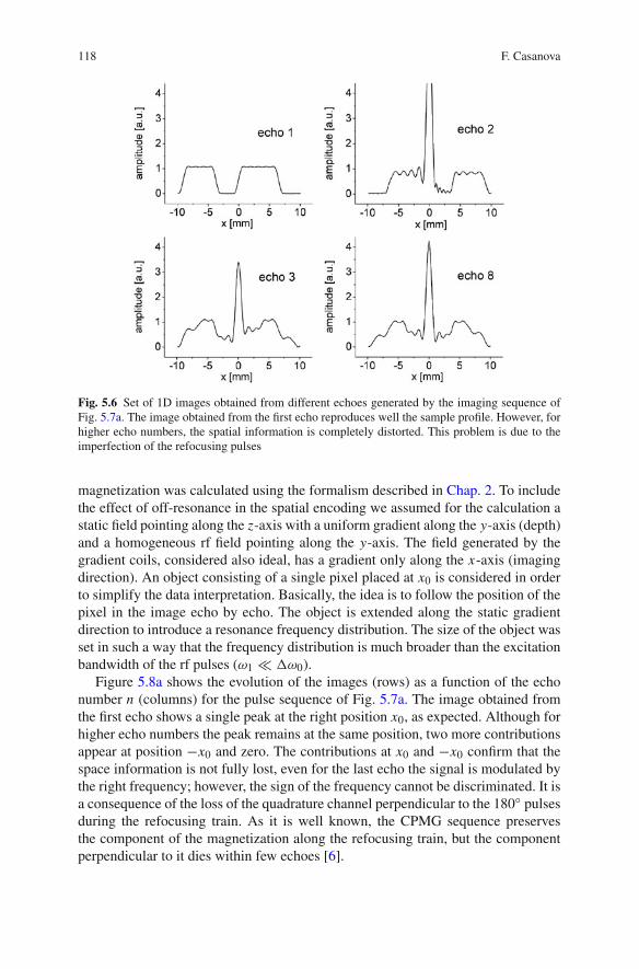
Fig. 5.7 (a) Straightforward extension from single- to multi-echo detection of the phase-encodingimaging sequence originally implemented in [4]. (b) The phase introduced by the first gradientpulse is canceled by a second one applied with opposite current. Therefore the phase distributionat the end of each evolution period is identical to the one obtained in the CPMG sequence. Bydoing so no spatial information must be preserved from echo to echo and the high performance ofthe CPMG sequence to generate a long echo decay is preserved

Although in the sequence of Fig. 5.7a the 180◦ pulses are applied 90◦ phaseshifted with respect to the first pulse, the gradient pulse rotates the magnetizationout of this direction generating a parallel and a perpendicular component. The lossof the perpendicular component (imaginary channel) leads to a mirroring of theimage. In the other hand, the contribution at zero frequency (x = 0) corresponds tosignal that is not affected by the gradient pulse. It comes from the stimulated echothat is stored as longitudinal magnetization during the application of the gradientpulse. Although the amplitude of the distortion at zero frequency is only one-half of

120 F. Casanova

Fig. 5.8 (a) Evolution of the image (rows) of a single pixel as a function of the echo numbern (columns) for the pulse sequence of Fig. 5.7a. The image obtained from the first echo shows,as expected, a single peak at the right position x0. Although for higher echo numbers the peakremains at the same position, another two contributions at −x0 and zero can be observed. (b) Byimplementing independent phase encoding of each echo (pulse sequence of Fig. 5.7b) all imagesare free of distortions

the amplitude at the correct position, the ratio becomes much larger when an objectwith many pixels is imaged. Notice that signal from every pixel of the image willcontribute to the zero frequency peak, leading in a general case to a huge distortionat the central position (Fig. 5.6). Although phase cycling could eliminate the signalarising from the stimulated echo, it would not solve the mirroring problem.

Once it was understood that the distortion was actually coming from magnetiza-tion dephasing introduced by the gradient pulse, a simple solution was presented.It used a second gradient pulse of polarity opposite to the first one to cancel thephase spread right after acquisition of the echo signal [7]. Thus, the magnetizationbefore the next refocusing pulse is exactly the same as in a normal CMPG sequence,and it can be preserved during the train. The procedure is repeated for every echoleading to the imaging sequence shown in Fig. 5.7b. Figure 5.8b shows the result ofimplementing the new sequence for the case of the single pixel object. The spatialinformation is perfectly encoded for all echoes; neither distortions at the mirrorposition nor zero frequency is observed. The amplitude of each gradient pulse canbe set equal in all the intervals, sampling the same k-space point for all the echoesof the train or it can be stepped to sample the complete k-space in a convenientway during a CPMG train decay. When the same k-space point is sampled in allthe echoes a set of experiments must be repeated, increasing the amplitude of thegradient pulses step by step to sample the complete k-space.

The echoes sampled during the decay can be added to improve the signal-to-noiseratio (Fig. 5.9a). In the case that T2 changes across the object the addition of allechoes acquired during the train decay results in a T2-weighted profile, while if aprofile is reconstructed from each echo it can be plotted as a function of the timeto determine the relaxation rate pixel by pixel. By changing the phase-encodingscheme, each echo can be used to sample a different k-space point scanning the com-plete image in a single CPMG train. As small values of k determine the amplitudeof the image, and the large ones determine the resolution, enhanced T2 contrast can


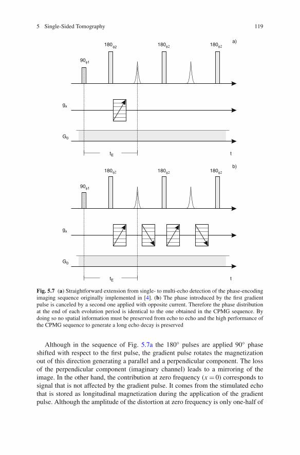
Fig. 5.9 (a) 1D images obtained by implementing the multi-echo pulse sequence shown inFig. 5.7b. On top the result obtained from the first echo (single-echo detection) and on the bot-tom from the addition of the complete echo train. (b) Taking advantage of the independent phaseencoding achieved in each echo, a RARE-type k-space sampling scheme was implemented toobtain T2-weighted 1D profiles. To compare the contrast the k-space was sampled from zero tokmax (top), and from kmax to zero (bottom)

be obtained in a single CMPG experiment by sampling the k values from maximumto zero (Fig. 5.9b). To obtain the maximum number of echoes during the CPMGsequence a short echo time is desired, but it is limited by the rise and fall times ofthe gradient pulses. The phase defined by the gradient pulse applied before eachecho must be completely canceled by the gradient pulse applied following the echo.This condition determines that the echo time must be long enough to assure thesecond gradient pulse to be zero when the next rf pulse is applied. If this is notfulfilled, a slightly different FOV is obtained from even and odd echoes, a fact thatcan be used to set the correct echo time. Depending on the T2 values, use of a currentpre-emphasis is needed to shape the current pulse.

5.3.2 CPMG-CP for Quadrature Detection

Shortly after the implementation of the RARE-like sequence a more powerfulmethod was presented [8]. In contrast to the first solution, where the magnetizationis spread and refocused before and after each echo without affecting the dynamics

122 F. Casanova

gx

gy

tEEtED t

G0

180

90 1

180

Fig. 5.10 CPMG-CP multi-echo sequence applied to sample the complete echo train decay. Bothgradient pulses are applied simultaneously during the free evolution periods of the Hahn-echosequence determining the encoding echo time tEE. To maximize the number of echoes that can begenerated during the detection period, the echo time is reduced after the formation of the first echo.The detection echo time tED is determined by the dead time of the probe

of the CPMG sequence, the second alternative exploits the fact that a CPMG trainat least preserves one component accepting that the second component is lost. Itrequires the combination of two experiments to acquire both quadrature compo-nents, but it increases the sensitivity by maximizing the number of echoes that canbe generated during the train and minimizes the power dissipated by the gradient coilsystem. The new pulse sequence (Fig. 5.10) can be understood as the combination ofa first encoding period consisting of a Hahn-echo sequence followed by a detectionperiod composed of a train of refocusing pulses.

The encoding period generates an echo signal with a phase defined by the pulsedgradients and the position of the spins. Then, for a given phase φ measured fromthe x-axis (here we assume that the Hahn echo is generated along the x-axis inthe absence of pulsed gradients, for example, applying the 90◦ with phase π/2 andthe 180◦ with phase 0) the components of the magnetization at the echo maximaare Mx = M0 cos(φ) and My = M0 sin(φ), with x- and y- directions in the rotat-ing frame (Fig. 5.11a). A first experiment executed with refocusing pulses appliedwith phase 0 (CPMG sequence) is used to sample Mx (real channel), while My

is attenuated to zero after a few pulses (Fig. 5.11b). The second experiment isidentical but the refocusing pulses are applied with phase π/2 (CP sequence) topreserve My (imaginary channel) (Fig. 5.11c). By combining the real componentof the first experiment with the imaginary of the second one the full complex signalM0(cos(φ)+i sin(φ)) is built for each echo. A typical experiment uses add–subtractphase cycling, so a minimum of four phase steps is required (see Table 5.1).


Fig. 5.11 (a) Magnetization vector at the time of the first echo maximum. The phase shift φ isproportional to position and the gradient strength. (b) During the application of the refocusingtrain with phase π/2 only My is preserved. (c) By switching the phase of the refocusing train to 0it is possible to preserve Mx

Table 5.1 Phase cycle required by the CPMG-CP sequence to sample both channels. It alsoincludes an add/subtract step

φ1 φ2 φα φrec Component

+π/2 0 0 0 Real−π/2 0 0 π Real+π/2 0 π/2 0 Imaginary−π/2 0 π/2 π Imaginary

Figure 5.12 shows a set of 1D images (obtained by numerical simulations) plot-ted as a function of the echo number for the new multi-echo detection scheme. Theconditions assumed are the same as in the previous calculations, off-resonance exci-tation and homogeneous B1. All images show the structure of the sample provingthat the space information is well preserved from echo to echo. As described inChap. 2, due to the superposition of the Hahn and the stimulated echo stored alongz by the second pulse, the CPMG train shows always a second echo larger than thefirst one. However, the sequence shown in Fig. 5.10 generates a second echo smallerthan the first one and a third echo larger than the second one. It is so because astED � tEE the first stimulated echo is lost (the second echo is only a direct echo),and the third echo is the first one where a stimulated echo (magnetization storedalong z by the first pulse of the detection train) superimposes with a Hahn echo.Notice that due to the large offset from resonance even with a homogeneous B1field, the refocusing pulses introduce a broad distribution of flip angles. Therefore,no significant changes are expected for the case of inhomogeneous B1 field.

In Table 5.2 the single-echo detection (Hahn echo) and the two multi-echo detec-tion sequences (RARE like and CPMG-CP) are compared in terms of measuringtime, average power, and total energy required. In favorable cases, where T2 is muchlonger than the echo time, the experimental time reduction obtained when movingfrom single- to the multi-echo detection can be several orders of magnitude. Theimprovement from 100 to 15 min achieved when the CPMG-CP sequence is usedinstead of the RARE-like one is due to the fact that for the first one the echo timein the detection train is limited only by the dead time of the rf probe, while in the

124 F. Casanova

Fig. 5.12 Set of 1D images acquired as a function of the echo number for the CPMG-CP multi-echo detection scheme (Fig. 5.10). All images show the structure of the object assumed for thecalculation proving that the space information is well preserved from echo to echo. The oscillationof the amplitude with the echo number is due to splitting of the signal in Hahn and stimulatedechoes, a typical behavior observed in CPMG-like sequences

Table 5.2 Comparison of the Hahn echo, RARE like, and CPMG-CP methods

Sequence Experimental time RF power (W) Gradient power (W) Energy (kJ)

Hahn echo 43 h 0.002 0.4 62RARE 100 min 0.1 47 282CPMG-CP 15 min 1.4 0.4 1.6

second one it is limited by the length of the two gradient pulses. The shorteningof the echo time increases the number of echoes that can be acquired during thetrain, maximizing the sensitivity enhancement. The important reduction of the totalenergy required is because only one instead of 2N gradient pulses is required pertrain of N echoes. This is an important issue determining the autonomy for portablesystems where the energy is stored in batteries. Besides these advantages, the mostimportant one is the ability of the CPMG-CP scheme to preserve phases defined inthe spin system prior to the application of the detection train, something that theRARE sequence cannot do. It allows that one can attach this acquisition scheme toany encoding sequence like the ones used for flow measurements described in thenext section.


5.4 Performance of the Multi-Echo Detection Scheme

5.4.1 Sensitivity Improvement

The time reduction that can be achieved with the new multi-echo technique insteadof the Hahn-echo sequence becomes significant for samples having long T2. Toshow the improvement obtained with the new sequence a silicone rubber samplewith T1 = 330 ms and T2 = 90 ms was imaged (Fig. 5.13a). It was positionedabove the sensor centered at 5 mm from the surface and a slice 1 mm thick wasselected. The sequence of Fig. 5.10 was implemented using gradient pulses 0.37 mslong and an echo time tED of 0.11 ms. The gradient amplitude was increased in 32steps sampling k-space from negative to positive values. The FoV was set to 32 mmalong both directions to obtain a spatial resolution of about 1 mm. A single scan wasused per gradient amplitude, and 800 echoes were acquired and averaged to improvethe signal-to-noise ratio. A recycling delay of 0.45 s was used between experimentsresulting in a total experimental time of 15 min to obtain a 2D image.

Fig. 5.13 (a) (Top). Geometry of a test object made of silicon rubber. (Bottom) 2D image obtainedby applying the new multi-echo acquisition scheme. Thanks to the 800 echoes generated duringthe echo train decay, a single scan per gradient amplitude was needed to sample each quadraturechannel. The echo train was sampled until the amplitude had decayed to 30% of the initial ampli-tude and before adding the echo train it was apodizated by the same decay function. The totalexperimental time to obtain the 2D images with a spatial resolution of about 1 mm was 15 min,reducing the acquisition time by a factor of 175 compared to the single-echo method, which wouldrequire 43 h. (b) Subtraction of the image of (a) from the image of a uniform object 50 × 50 mm2

used to probe the FoV defined by the RF coil. The dimensions of the selected sensitive volume are36 mm along x and 26 mm along z

126 F. Casanova

Figure 5.13a shows the cross section obtained using the new pulse sequence. Theimage reproduces the structure of the object without appreciable distortions demon-strating that 2D spatial localization can be obtained across the selected slice [8]. Toobtain a 2D cross section with the same signal-to-noise ratio but using the single-echo sequence a larger number of scans must be used. As the amplitude of the echotrain decays exponentially and is sampled up to one-third of its initial amplitude, thesensitivity improvement can be easily calculated. For this rubber sample 175 fullHahn echoes must be averaged to obtain the signal-to-noise ratio provided by themulti-echo sequence, giving an experimental time of about 43 h. The field of viewdefined by the rf coil was probed by a uniform silicon rubber sample with dimen-sions 50 × 50 mm2 along the x- and z-axes. The fast imaging method was imple-mented using the parameters of the previous experiment, but a FoV of 42 mm wasset. Figure 5.13b shows the result obtained by subtracting the image of Fig. 5.13afrom the image of the uniform object. The RF coil defines a FoV of 36 mm alongx and 26 mm along z. In case a large object is positioned on the sensor, the FoVsmust be set larger than these dimensions to avoid folding of the signal. For thesake of simplicity, objects with limited sizes along x and z will be used from thispoint on.

5.4.2 Relaxation and Diffusion Contrast

As described above, the multi-echo imaging sequence is basically obtained by com-bining a Hahn-echo sequence and a CPMG-like multi-echo detection train. Thisfeature can be exploited to produce contrast in the image using the Hahn-echosequence as a filter or directly from the CPMG decay by considering different partsof the echo train. In the previous section the complete echo train was added for sen-sitivity improvement, but this approach leads to density images only if T2 does notvary across the sample. In case a distribution of T2 values is present, a T2-weightedimage is obtained. The way to maximize the contrast is to add different parts of thetrain. If, for example, domains with known T2 values are present in the sample, theintegration limits in the decay curve can be easily set to maximize the differencebetween the two signals, but if an unknown sample is to be studied, different partsof the train can be chosen with a judicious elections of the limits based on the overallsignal decay.

An application of this method is shown in Fig. 5.14a, where it was used to dis-criminate three different rubber types present in the object. A 1 mm thick slice at5 mm from the surface and inside the object was selected. The multi-echo sequencewas applied setting tED = 0.11 ms and using 1,000 echoes to correctly samplethe longest decay present in the object. The gradient amplitude was increased in24 steps and with the FoV set to 32 mm a spatial resolution of about 1.3 mm wasobtained. The repetition time was set to 0.3 s, three times the longest T1 to avoid anyT1 weighting in the image. Eight scans were averaged for sensitivity improvement.Figure 5.14a shows different T2-weighted images reconstructed from the addition


Fig. 5.14 (a) Object geometry composed of three different kinds of rubber presenting differentrelaxation times. To produce different T2 contrast different train intervals were averaged beforeimage reconstruction. The set of images (from left to right) was obtained by adding the echoes1–8, 8–32, 100–200, and 200–400. (b) Amplitude decays corresponding to the three characteristicregions inside the object. Fitting the decaying signal in each pixel the local relaxation time wasobtained. The values shown in the picture are in agreement with the relaxation times of each rubbersample

of the echoes (from left to right) 1–8, 8–32, 32–200, and 200–400. Normalizing thehighest intensity of each image to one, the first image shows the rectangular objectwith almost uniform intensity, the second one shows the shortest T2 region with halfof the maximum intensity, while the other two regions cannot be differentiated, thethird one shows the shortest T2 with zero intensity, the middle one with the half ofthe intensity, and the longest with full intensity, and finally in the last image onlythe region with the longest T2 is visible. Instead of adding parts of the echo train toproduce contrast in the images the local relaxation time can be obtained by fittingthe amplitude decay of each pixel. In contrast with the single-echo method the com-plete decay is sampled in a single imaging experiment, reducing the dimensionalityof the experiment by one. Figure 5.14b shows the signal decays corresponding toeach region in the object together with the respective fit. From dark to light graythe obtained relaxation times are 1.9, 5, and 15 ms, in agreement with the relaxationtimes measured from each single rubber sample using a CPMG sequence.

In cases where different regions in the sample possess similar CPMG decaytimes, but different signal attenuation during the Hahn-echo sequence, the encodingecho time (tEE) can be purposely increased to enhance the contrast between them.

128 F. Casanova

W O

G

Fig. 5.15 Phantom composed of three tubes filled with water, oil, and gelatin. The imagingsequences allow to introduce contrast by diffusion by increasing the encoding echo time tEE. Fromleft to right the images were measured with tEE = 0.5, 1, 2, and 5 ms. During the detection period1,000 echoes were generated and co-added for sensitivity improvement. While the first imagedoes not show any contrast between the tubes, for longer encoding times the contrast introducessignal attenuation for the water and gelatin sample, while almost no attenuation is observed for theoil tube

This approach is ideal, for example, to produce contrast by diffusion in liquid-likesamples. In this case the signal intensity is strongly attenuated by diffusion duringthe encoding period, while for short enough detection echo times the CPMG decaysmight be similar. It must be noticed that increasing tED to enhance diffusion contrastduring the CPMG decay is disadvantageous because it leads to SNR deteriorationin the image due to a reduction in the total number of echoes that can be acquiredduring the detection period. Figure 5.15 shows images of three tubes filled withwater, oil and gelatin. They were measured using encoding times of tEE = 0.5, 1, 2,and 5 ms (from the left to the right) and 1,000 echoes during the acquisition train.It can be nicely observed that for short tEE the method allows the measurement ofdensity images, while for longer values important contrast can be produced keepingthe sensitivity improvement achieved by adding the long echo train. The method hasproven to be of great help discriminating fat and meat in biological tissue, resultsthat are presented in Chap. 8.

5.4.3 3D Imaging

Combining the 2D phase-encoding method with slice selection, 3D spatial reso-lution is achieved [8]. Figure 5.16a shows an object with a 3D structure obtainedby stacking a set of letters forming the word MOUSE cut from a sheet of 2 mmthick natural rubber. Having no spacer in between the letters the total structure is10 mm high. For a better view, Fig. 5.16b shows the letters separated one fromeach other. After calibrating the frequency dependence with the position along thedepth direction different 1 mm thick slices were selected, one inside each letter. Thenew multi-echo acquisition scheme was applied using 20 gradient steps and a FoVof 32 mm, giving a spatial resolution of about 1.6 mm. To have the same FoV atdifferent depth both gradient amplitudes were calibrated. For this rubber sample,96 echoes were added for sensitivity improvement. Using a recycle delay of 30 msand two scans an experimental time of 45 s was needed to obtain the image of thefirst letter. To compensate the loss of sensitivity due to B1 reduction as a function ofdepth, an increasing number of scans was used for the next letters needing a factor


Fig. 5.16 (a) Object made by stacking the letters of the word MOUSE cut from a rubber sheet2 mm thick. (b) Expanded view of the object obtained by drawing the letters separate from eachother to see the object structure. (c) Images of each letter obtained by applying the multi-echoimaging method and selecting a 1 mm thick slice in the center of each letter. To compensate for theloss in sensitivity due to the B1 decay, the number of scans used for each letter was increased pro-portional to depth. The total time to obtain each letter was 45, 45, 90, 120, and 180 s, respectively

of 4 for the last one. The 2D image of each letter can be observed in Fig. 5.16c.The flatness of the sensitive volume is good enough to observe no superpositionof consecutive letters, and as no distortions can be observed in any of them weconclude that the uniformity of the pulsed gradients is acceptable in the completerange.

5.5 Displacement Encoding

Nuclear magnetic resonance has proved to be a powerful tool to characterize molec-ular motion non-invasively [1, 2]. It is suited to study displacement in a wide rangeof time and length scales. For opaque materials, for which optical methods areexcluded, there are few experimental methods able to determine molecular displace-ments in any detail. NMR techniques offer a number of advantages compared toother experimental methods [9] and have been widely used in biology, medicine,and material science. NMR has enabled, for example, the measurement of vascularflow in stems and petioles at various stages of plant development, as well as vascularblood flow during the cardiac cycle. Also numerous applications in porous mediasuch as natural sandstone have helped to elucidate models that describe the transportof fluids within the porous structure [10]. Combined with high-resolution imagingmethods, it is a unique experimental method to check numerical solutions to theNavier–Stokes equation for Newtonian liquids or to validate constitutive equationsused to describe the complex rheological behavior of non-Newtonian fluids [11, 12].In contrast to other methods it is not affected by the vicinity of walls, providing, forexample, the possibility to study effects such as the wall slip observed in the velocityshear of polymer melts and solutions [13].

130 F. Casanova

A number of sequences based on the use of pulsed field gradients (PFG) havebeen implemented and tested in the homogeneous field of conventional supercon-ducting and electromagnets, but several problems appear when they are imple-mented in the extremely inhomogeneous fields of open sensors. First, dependingon the sequence, the strong static gradient G0 of the main field can introduce sig-nificant signal attenuation due to molecular self-diffusion. Second, off-resonanceexcitation and rf field inhomogeneity lead to a large number of coherence pathwayswith improper displacement encoding. Third, the low magnetic field strength andthe broadband signal inherent to these sensors yield low sensitivity and extend theexperimental times to unviable limits. In this section a modification to the PFG-stimulated spin echo of Tanner [14], the so-called 13-interval sequence proposed byCotts [15], is described. In particular, a phase cycling designed to eliminate spuriouscoherence pathways is given. This sequence reduces the signal loss due to diffusionin the presence of the strong background gradient and can be combined with themulti-echo detection CPMG-CP scheme to reduce the experimental time by severalorders of magnitude, allowing the measurement of velocity distributions in a fewminutes. Furthermore, this flow-encoding method can be combined with imagingtechniques to spatially resolve velocity distributions and to obtain 2D velocity mapsin situ.

5.5.1 PFG Methods in Inhomogeneous Fields

PFG methods measure coherent and diffusive displacement by means of spin echoes(SE) [16] and stimulated echoes (STE) [14] formed in the presence of pulsed fieldgradients. In systems where T2 is much shorter than T1, the PFG-STE sequence ofTanner has proven to be better suited than the conventional PFG-SE sequence. Fig-ure 5.17a shows Tanner’s sequence, where two gradient pulses of length δ separatedby an evolution time� are applied to introduce phase shifts φi and φf proportional tothe initial and final positions ri and rf [17]. As the magnetization is stored along thelongitudinal axis during the evolution period �, PFG-STE allows longer evolutioninterval between the encoding and decoding gradient pulses (Fig. 5.17a). In this waythe relaxation rate during the evolution period is given by T1 and not by T2 as in theSE sequence.

In the presence of a static magnetic field gradient G0, the echo signal generatedby the PFG-STE sequence is attenuated by diffusion as [14]

ln(M(t)/M0) = −γ 2 D{δ2(�+ τ − δ/3)g2

1

+ δ(2τ�+ 2τ 2 − 2/3δ2 − δ(δ1 + δ2)− (δ2

1 + δ22))g1G0

+ τ 2(�+ 2/3τ)G20

}, (5.1)

where τ is the time between the first two 90◦ pulses and δ1,2 are the times betweenthe rf and the gradient pulses. Depending on the G0 value significant attenuation can


t

tE

Encoding Detection

t

a)

b)

g1

g1

G0

G0

9090 1

180

90 1

90

90 3 90 4

180 180

Fig. 5.17 (a) Stimulated spin-echo PFG sequence to measure displacement during the free evo-lution period �. (b) 13-interval PFG-STE sequence (encoding period) that cancels the effect ofthe strong static gradient generated by the open magnet geometry. Refocusing pulses are appliedduring the coding intervals to cancel the phase spread due to the static gradient. To increase thesensitivity a train of rf pulses (detection period) is applied after formation of the stimulated echo.The echo time tED for detection is determined by the dead time of the probe

be expected [15, 18]. This fact complicates, and in some cases prevents, the use ofthis method for displacement encoding in the presence of background gradients. Toreduce the diffusive signal attenuation due to G0, Cotts et al. developed the so-called13-interval sequence, denoted as encoding period in Fig. 5.17b [15]. It includes 180◦pulses applied during the coding intervals to cancel the phase spread introduced byG0 during each of these periods, while the encoding phase is defined by means ofbipolar gradient pulses. For this sequence the signal attenuation due to moleculardiffusion is

132 F. Casanova

ln(M(t)/M0) = −γ 2 D{δ2(4�+ 6τ − 2/3δ)g2

1 + 2τδ(δ1 − δ2)g1G0

+ 4/3τ 3G20

}. (5.2)

In contrast to the PFG-STE sequence, signal attenuation due to diffusion underG0 arises only during the two encoding periods, but not during �. The sequencehas been widely applied to measure flow in heterogeneous samples such as porousmedia showing that distortions introduced by field inhomogeneities can be consid-erably reduced.

Unfortunately, the application of this sequence with an open sensor, where the B0and B1 fields are strongly inhomogeneous requires important analysis. The complexdistribution of flip angles across the sensitive volume generates a large number ofcoherence pathways (35) that must be filtered by phase cycling. In order to keep thenumber of phase steps to a minimum it is important to notice that several of thispathways will have negligible contribution and can be simply ignored. This is thecase of the magnetization evolving in the transverse plane during �. In a typicalexperiment this evolution time is much longer than τ and of the order of severalmilliseconds, so transverse magnetization is strongly attenuated by T2 and diffusion.From the pathways evolving with q3 = 0 only the six listed in Table 5.3 fulfill theecho condition described by Eq. (2.12).

The first two are both generated even when the sequence is implemented underon-resonance condition and homogeneous B1 field and superimpose during signaldetection. As the phase accumulated during a free evolution period qk is propor-tional to qk (see Chap. 2), for the case where the gradient pulses are applied with thepolarities shown in Fig. 5.17b, P1 is modulated by a phase (φi − φf) proportional tothe average displacement and P2 by a phase (−φi − φf) proportional to the averageposition. When the signal is sampled as a function of the gradient strength bothcontributions are present, and a superposition of the velocity distribution and theimage of the sample are obtained (Fig. 5.18a). To cancel the contribution of P2,the dependence of the pathways on the phase of each rf pulse must be exploited.For example, it can be eliminated stepping the phases of the third and fourth pulsesfrom 0 to π/2 and keeping the receiver phase constant [19] (Fig. 5.18b). In this case,P1 does not change, but the signal coming from P2 shift π and cancel out after twoscans.

The rest of the pathways are present only when the sequence is imple-mented under non-ideal experimental conditions, so their contribution to the final

Table 5.3 Pathways interfering during the acquisition period of the 13-interval sequence

Pathway Phase

P1 = M0,+1,−1,0,−1,+1 +φ1 − 2φ2 + φ3 − φ4 + 2φ5P2 = M0,−1,+1,0,−1,+1 −φ1 + 2φ2 − φ3 − φ4 + 2φ5P3 = M0,−1,−1,0,+1,+1 −φ1 + φ3 + φ4P4 = M0,−1,0,0,0,+1 −φ1 + φ2 + φ5P5 = M0,0,−1,0,0,+1 −φ2 + φ3 + φ5P6 = M0,0,0,0,−1,+1 −φ4 + 2φ5


0.0

0.5

1.0

–4 –2 0 2 4

–40 –20 0 20 40–40 –20 0 20 40

0.0

0.5

1.0

position [mm]am

plitu

de [a

.u.]

velocity [mm/s]

ampl

itude

[a.u

.]

velocity [mm/s]

b)a)

Fig. 5.18 (a) Simulated velocity profile for the 13-interval sequence (Fig. 5.17a). A single velocityof 20 mm/s inside a slice 2 mm thick and perpendicular to the flow direction was assumed. Not onlya single velocity is obtained, but also the image of the slice is observed. (b) The unwanted imageis completely removed by cycling the phases of the second rf pulse from 0 to π/2, keeping thereceived phase unchanged

signal depends on the particular sensor. To understand the performance of the pulsesequence, the signal response was calculated as a function of the effective flip angle(θ ) assuming a single velocity v. This simulation cycles the phases needed to can-cel the contribution of P2, which at the same time eliminates P3 (this path is noteffectively encoded by the bipolar gradients because the 180◦ pulses applied in eachcoding period do not invert the sign of the accumulated phase). Figure 5.19 showsthe velocity distribution obtained as a function of the flip angle. For θ values close to90◦ the profile is undistorted and the single velocity is at the right spectral position.Nevertheless, when θ deviates from the ideal value ( because either of B1 or Boffvariations), a spurious contribution at half the original velocity value is obtained.This peak is the magnetization encoded by only one of the two gradient pulsesduring each coding period, which is modulated with half of the correct frequency inthe q-space.

The pathway responsible for this spurious signal is the P5, which is encoded witha phase (φini/2 − φfin/2). (As q2 = −1 a positive initial phase is acquired duringq2 where the gradient pulse is negative, but a negative phase is acquired during thefifth period where q5 = +1 and the gradient pulse is negative). In order to quantifythe importance of this distortion for the conditions of a real experiment we includedin the calculations the off-resonance excitation and the real B1 distribution of therf coil. Figure 5.20a shows the obtained velocity distribution. The peak at v/2 isclearly observed and its relative amplitude is almost 50% compared to the amplitudeat the correct velocity. As observed in Fig. 5.19, the distortion is the largest for flipangles close to π/4. For this value a large component of the magnetization remainsalong the z-axis after the application of the first rf pulse and is not encoded by thefirst gradient pulse of the encoding period. This remnant component is eliminatedby cycling the phase of the first rf pulse and the phase of the receiver from 0 to π

134 F. Casanova

0 v/2 v

velocity

flipangle

Fig. 5.19 Velocity profiles obtained as a function of the flip angle. For the calculation homo-geneous static and rf fields were assumed as well as a uniform velocity v. A correct velocitydistribution is obtained for flip angles close to 90◦, while the profiles become distorted for flipangles close to 45 and 135◦

(add–subtract phase cycling) [19]. This phase cycle also eliminates P6 and the freshmagnetization created during �. Figure 5.20b shows the velocity profile obtainedby including this phase cycle in the simulation. The distortion is clearly absent. Toremove the remaining pathway P4, which is encoded with a phase proportional tohalf of the average position (−φini/2−φfin/2), φ2 must be cycled from π/2 to −π/2keeping the receiver phase constant. However, it does not appear to introduce bigdistortions, so these steps are not included in Table 5.4.

Besides the mentioned distortions that appear as a consequence of the field inho-mogeneity, the use of this technique is limited by the poor sensitivity of single-sidedsensors. In Sect. 5.2.2 the use of the multi-echo acquisition scheme CMPG-CPfor sensitivity improvement was described. Figure 5.17b shows that it can also beattached to the 13-interval sequence (encoding period). As already mentioned, the

–20 –10 0 10 20 –20 –10 0 10 20

0.0

0.5

1.0

0.0

0.5

1.0

ampl

itude

[a.u

.]

velocity [mm/s]

ampl

itude

[a.u

.]

velocity [mm/s]

b)a)

Fig. 5.20 (a) Velocity profiles calculated considering both the off-resonance due to the static gra-dient of the sensor and the B1 field distribution provided by the rf coil. Although a single velocityof 20 mm/s was assumed in the simulation, a contribution at half of this value is also observed.(b) To effectively cancel this distortion, the phase of the first rf pulse and the receiver phase werecycled from 0 to π


Table 5.4 Phase cycle to filter unwanted pathways generated when the 13-interval sequence isapplied in inhomogeneous fields

φ1 φ2 φ3 φ4 φ5 φα φrec

0 π/2 0 0 π/2 π/2 00 π/2 π/2 π/2 π/2 π/2 0π π/2 0 0 π/2 π/2 π

π π/2 π/2 π/2 π/2 π/2 π

0 π/2 0 0 π/2 0 00 π/2 π/2 π/2 π/2 0 0π π/2 0 0 π/2 0 π

π π/2 π/2 π/2 π/2 0 π

refocusing pulses only preserve the component of the echo signal parallel to therefocusing rf pulses, while the perpendicular component goes to zero after a tran-sient period. For the reconstruction of the velocity distribution both magnetizationcomponents are necessary and the loss of one of them mirrors the spectrum. Tosample both components two experiments are performed, switching the phase ofthe rf pulses of the refocusing train from 0 to π/2. In summary, the total experimentrequires a minimum of eight scans per gradient step. The phase of the first rf pulsemust be cycled from 0 to π to eliminate distortions due to the flip angle distribution,the phase of the third and fourth rf pulses from 0 to π/2 to eliminate the unwantedimage from the velocity profile, and the sequence must be repeated changing thephase of the refocusing train to sample both components of the echo signal (seeTable 5.4). It should be noticed that under strong background gradients and longenough � the unwanted pathways can be strongly attenuated because for them the13-interval sequence is actually a stimulated echo sequence (only three of the fivepulses act on the magnetization) where diffusion attenuation during � is observed.

5.5.2 Measurement of Velocity Distributions

The new flow-encoding method was implemented on the open tomograph describedin Chap. 4. Its efficiency to remove the effect of the background gradient was testedfirst. The sequence was implemented without gradient pulses, and the echo inten-sity from water doped with Cu2S was sampled as a function of � for different δvalues. The acquired decays could be fitted by a mono-exponential function with atime constant independent of δ and equal to T1 in all cases. This result proves thatthe stimulated echo stored as longitudinal magnetization during � is free of phasecontributions introduced by the static gradient.

To illustrate the performance of the method, the water flow in a thin rectangularpipe was measured. The tube, 12 mm wide, 0.6 mm high, and 200 mm long, wasplaced at 10 mm from the sensor surface. When the ratio between the height a andthe width b of the tube is b/a � 1, the velocity profile of laminar flow can be consid-ered to be flat along the long side b while it changes quadratically with the height a[20]. A volume flow rate Q of 170 ml/h was driven by a precision pump Pharmacia

136 F. Casanova

–15 –10 –5 0 5 10 15

0.0

0.5

1.0

1.5experimenttheory

ampl

itude

[a.u

.]

velocity [mm/s]–0.5 0.0 0.5 5 10 15 20

–0.5

0.0

0.5

5

10

15

20 experimentlinear fit

v NM

R[m

m/s

]

va

[mm/s]

a) b)

Fig. 5.21 (a) Velocity distribution of water flowing in a rectangular pipe obtained with the pulsesequence of Fig. 5.17b. Dots denote experimental data. The water used for the experiment wasdoped with Cu2S to reduce the T1 value to 0.9 s. The gradient pulse length δ was set to 0.5 msand the evolution period � to 200 ms. To improve the signal-to-noise ratio 2,000 echoes wereacquired with tED = 0.11 ms. The total experimental time to obtain the velocity distribution work-ing at 10 mm from the sensor surface was 5 min. For comparison the theoretical distribution wascalculated and is shown as a continuous line. (b) Correlation between the average velocity vNMRmeasured using the single-step phase-encoding PFG-STE method with the value va, determinedfrom the known flow rate and the geometry of the tube

P500 defining a maximum velocity vm = 3/2 × Q/(ab) of about 10 mm/s. Thedotted velocity profile in Fig. 5.21a was measured with the sequence of Fig. 5.17b.The q-space was sampled in 24 steps from negative to positive values and with thefield of flow set to 30 mm/s, a velocity resolution of about 1.25 mm/s was defined.To excite all the spins across the tube, the length of rf pulses was set to 7 μs defininga slice thickness of about 1.4 mm. The shortest echo time tED = 0.11 ms, limitedby the dead time of the probe, was employed. A train of 2,000 echoes was addedto improve the sensitivity by a factor of 20 compared to single-echo detection [19].Thanks to this dramatic sensitivity enhancement, only eight scans were required,determining a total time of about 5 min to measure the velocity distribution. Thetheoretical velocity profile for this pipe geometry was calculated and is shown inFig. 5.21a as well. The good agreement between experimental and theoretical curvesproves that the method is suitable to remotely measure velocity distributions, evenin these extremely inhomogeneous fields.

Single-sided sensors are usually repositioned to scan the object at different spots.In some applications only the average velocity at each spot is required. When thisis the case a single phase-encoding step can be used instead of the N steps neededto reconstruct the full propagator [21]. The sacrifice in velocity resolution leads to adirect reduction in experimental time by a factor of N/2. The procedure requires aninitial experiment without gradient pulses to measure the reference phase of the echosignal, and a second experiment with the gradient pulses to introduce a phase shift inthe echo proportional to the displacement. From this phase shift the average velocityinside the sensitive spot can be easily computed. The method was implemented tomeasure the average velocity va = Q/(ab) in the rectangular pipe. Figure 5.21b


shows the average velocity vNMR measured with the single-step PFG-STE method asa function of the average velocity calculated via the known flow rate. The excellentcorrelation proves that the method is accurate in a wide velocity range. The time tomeasure the average velocity inside the selected volume, under the same conditionsas in the previous experiment, was about 24 s.

5.6 Spatially Resolved Velocity Distributions

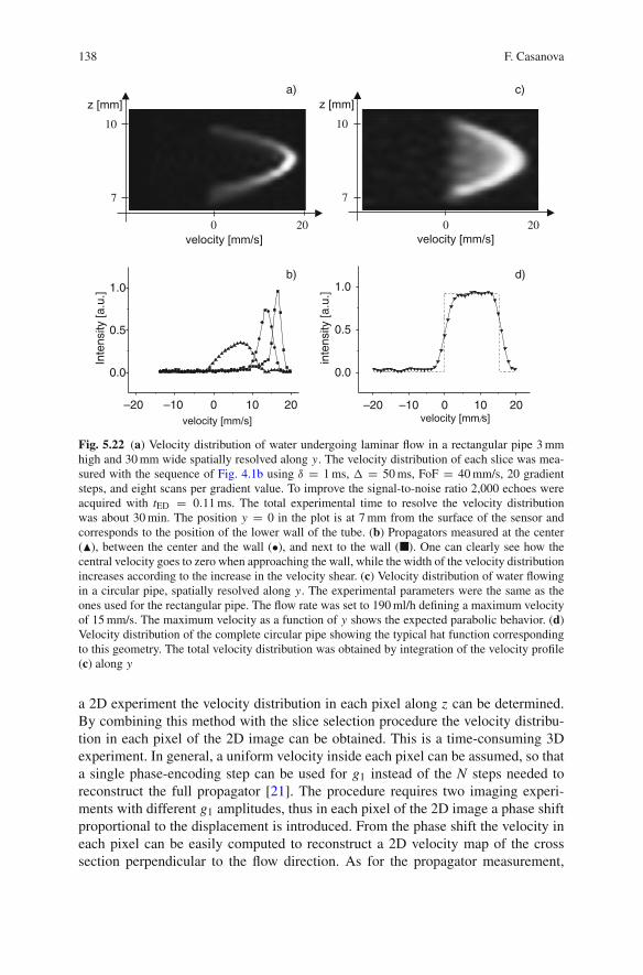
In this section the method developed to encode velocity is combined with a sliceselection procedure to spatially resolve the velocity profile in the object along thedepth direction. Flat slices at different depths can be selected by stepping the exci-tation frequency as was shown in the previous sections (Fig 5.16). To illustrate theperformance of the method, the profile of water flowing in a rectangular pipe 30 mmwide, and 3 mm high was measured. A volume flow rate of 3,600 ml/h was drivenby a precision pump, defining a maximum velocity in the pipe of about 17 mm/s.When the ratio b/a between the height and the width of the tube is much larger than1, the velocity of laminar flow can be considered to be constant along the long sideb while it changes as a quadratic function of the height a. The pipe was scannedalong y by sweeping the position of the sensitive slice in steps of 0.3 mm from 7to 10 mm, where the tube was placed. Figure 5.22a shows the spatially resolvedvelocity distribution where the parabolic profile is clearly visible [22]. Figure 5.22bshows the propagators measured at three different positions in the tube. They showhow the averaged velocity in the slice goes to zero as the slice approaches the wall,while the width of the distributions increases, in agreement with the change in thelocal shear value.

As a second example the velocity distribution of water flowing in a circular pipewith 3 mm inner diameter was scanned with the same experimental parameters asbefore. Figure 5.22c shows the propagator spatially resolved along y [22]. In con-trast to the rectangular geometry, for a circular pipe of radius R the velocity dependson both y and z as v(x, y, z) = vmax × (1 − (y2 + z2)/R2). This defines a veloc-ity distribution in each slice with velocity ranging from zero to a maximum valuethat depends on the y-position. The parabolic behavior of the maximum velocity isclearly resolved in Fig. 5.22c, where it can be also observed that the velocity proba-bility is non-zero from zero up to the maximum velocity in the slice. The completepropagator of the tube can be reconstructed by integrating the distributions alongthe depth direction. Figure 5.22d shows the characteristic hat function distributionexpected for this geometry.

5.6.1 2D Velocity Maps

Once a slice is selected, the velocity distribution can be resolved along a lateraldirection by including a pulsed field gradient gz in the sequence (Fig. 5.23) [22].Stepping the amplitudes of g1 (in this case applied along x) and gz independently in

138 F. Casanova

0 20

7

10

–20 –10 0 10 20

0.0

0.5

1.0

Inte

nsity

[a.u

.]

–20 –10 0 10 20

0.0

0.5

1.0

inte

nsity

[a.u

.]

0 20

7

10

a)

d)

c)

b)

Fig. 5.22 (a) Velocity distribution of water undergoing laminar flow in a rectangular pipe 3 mmhigh and 30 mm wide spatially resolved along y. The velocity distribution of each slice was mea-sured with the sequence of Fig. 4.1b using δ = 1 ms, � = 50 ms, FoF = 40 mm/s, 20 gradientsteps, and eight scans per gradient value. To improve the signal-to-noise ratio 2,000 echoes wereacquired with tED = 0.11 ms. The total experimental time to resolve the velocity distributionwas about 30 min. The position y = 0 in the plot is at 7 mm from the surface of the sensor andcorresponds to the position of the lower wall of the tube. (b) Propagators measured at the center(�), between the center and the wall (•), and next to the wall (�). One can clearly see how thecentral velocity goes to zero when approaching the wall, while the width of the velocity distributionincreases according to the increase in the velocity shear. (c) Velocity distribution of water flowingin a circular pipe, spatially resolved along y. The experimental parameters were the same as theones used for the rectangular pipe. The flow rate was set to 190 ml/h defining a maximum velocityof 15 mm/s. The maximum velocity as a function of y shows the expected parabolic behavior. (d)Velocity distribution of the complete circular pipe showing the typical hat function correspondingto this geometry. The total velocity distribution was obtained by integration of the velocity profile(c) along y

a 2D experiment the velocity distribution in each pixel along z can be determined.By combining this method with the slice selection procedure the velocity distribu-tion in each pixel of the 2D image can be obtained. This is a time-consuming 3Dexperiment. In general, a uniform velocity inside each pixel can be assumed, so thata single phase-encoding step can be used for g1 instead of the N steps needed toreconstruct the full propagator [21]. The procedure requires two imaging experi-ments with different g1 amplitudes, thus in each pixel of the 2D image a phase shiftproportional to the displacement is introduced. From the phase shift the velocity ineach pixel can be easily computed to reconstruct a 2D velocity map of the crosssection perpendicular to the flow direction. As for the propagator measurement,


t

tE

Encoding Detection

gvel

G0

180

90 1 90 3 90 4

180 180

gz

Fig. 5.23 Thirteen-interval stimulated spin-echo PFG sequence to measure displacement duringthe free evolution period �. The sequence includes a bipolar gradient pulse applied before thedetection train to obtain spatial resolution along z

a minimum of eight scans is required for the phase cycle to remove the distortionsand to sample the two components of the signal.

The method was implemented to map the velocity profile of a laminar water flowin a circular pipe with 6 mm inner diameter. The flow rate was set to 500 ml/h todefine a maximum velocity of about 10 mm/s. The pipe was scanned along y movingthe position of the sensitive slice in steps of 0.5 mm. A 1D profile along z of eachslice was obtained by increasing the amplitude of the pulsed gradient in 16 steps,setting a FoV of 8 mm, the same spatial resolution along both spatial directions wasdefined. Figure 5.24a shows the 2D velocity map computed from the pixel phaseshift measured with the single-step PFG-STE method. The plot clearly shows theannular pattern corresponding to the parabolic profile developed in this geometry.The agreement of the results with the theoretical profile can be judged in Fig. 5.24b,where the profiles along y and z are displayed together with the expected quadraticfunction.

The detailed information about fluid transport properties provided non-invasively, together with the simplicity of the measurement procedure, identifiessingle-sided NMR as a suitable technique to characterize flowing characteristics ofcomplex fluids. In this chapter, an alternate PFG-STE sequence suitable to encodedisplacement in the presence of strong B0 and B1 field gradients has been presented.It has been successfully implemented on a single-sided NMR sensor to measurevelocity distributions ex situ. As for imaging experiments, a key step to measurevelocity ex situ is the incorporation of the multi-echo acquisition scheme followingthe displacement-encoding period.

140 F. Casanova

–4 –2 0 2 4

0

5

10

v [m

m/s

]

position [mm]

–4 –2 0 2 4

4

6

8

10

y [mm]

z [m

m]

Fig. 5.24 (a) 2D velocity map of water flowing in a circular pipe, 6 mm in diameter. It was obtainedwith the pulse sequence of Fig. 5.23, using the single gradient step method to encode velocity. Thetotal experimental time to obtain the velocity distribution with the tube placed between 4 and10 mm from the sensor surface was 50 min. (b) Velocity profiles along y (�) and z (�) plottedtogether with the expected quadratic function (dashed line)

References

1. Callaghan PT (1991) Principles of nuclear magnatic resonance microscopy. Clarendon Press,Oxford

2. Blümich B (2000) NMR imaging of materials. Clarendon Press, Oxford3. Perlo J, Casanova F, Blümich B (2005, Sep) Profiles with microscopic resolution by single-

sided NMR. J Magn Reson 176(1):64–704. Prado PJ, Blümich B, Schmitz U (2000, June) One-dimensional imaging with a palm-size

probe. J Magn Reson 144(2):200–2065. Casanova F, Blümich B (2003, July) Two-dimensional imaging with a single-sided NMR

probe. J Magn Reson 163(1):38–456. Meiboom S, Gill D (1958) Modified spin-echo method for measuring nuclear relaxation times.

Rev Sci Instrum 29(8):688–6917. Casanova F, Perlo J, Blümich B, Kremer K (2004, Jan) Multi-echo imaging in highly inho-

mogeneous magnetic fields. J Magn Reson 166(1):76–818. Perlo J, Casanova F, Blümich B (2004, Feb) 3D imaging with a single-sided sensor: an open

tomograph. J Magn Reson 166(2):228–235


9. Xia Y, Callaghan P T, Jeffrey KR (1992, Sep) Imaging velocity profiles – flow through anabrupt contraction and expansion. Aiche J 38(9):1408–1420

10. Packer KJ, Tessier JJ (1996, Feb) The characterization of fluid transport in a porous solid bypulsed gradient stimulated echo NMR. Mol Phys 87(2):267–272

11. Arola DF, Powell RL, Barrall GA, McCarthy MJ (1999, Jan) Pointwise observations forrheological characterization using nuclear magnetic resonance imaging. J Rheol 43(1):9–30

12. Yeow YL, Taylor JW (2002, Mar) Obtaining the shear rate profile of steady laminar tube flowof newtonian and non-newtonian fluids from nuclear magnetic resonance imaging and laserdoppler velocimetry data. J Rheol 46(2):351–365

13. Xia Y, Callaghan PT (1991, Aug) Study of shear thinning in high polymer-solution usingdynamic NMR microscopy. Macromolecules 24(17):4777–4786

14. Tanner JE (1970) Use of stimulated echo in NMR-diffusion studies. J Chem Phys 52(5):2523–2526

15. Cotts RM, Hoch MJR, Sun T, Markert JT (1989, June) Pulsed field gradient stimulated echomethods for improved NMR diffusion measurements in heterogeneous systems. J Magn Reson83(2):252–266.

16. Stejskal EO, Tanner JE (1965) Spin diffusion measurements – spin echoes in presence of atime-dependent field gradient. J Chem Phys 42(1):288–292

17. Kimmich R (1997) NMR: tomography, diffusometry, relaxometry. Springer, Berlin18. Sun PZ, Seland JG, Cory D (2003, Apr) Background gradient suppression in pulsed gradient

stimulated echo measurements. J Magn Reson 161(2):168–17319. Casanova F, Perlo J, Blümich B (2004, Nov) Velocity distributions remotely measured with a

single-sided NMR sensor. J Magn Reson 171(1):124–13020. Gondret P, Rakotomalala N, Rabaud M, Salin D, Watzky P (1997, June) Viscous parallel flows

in finite aspect ratio hele-shaw cell: analytical and numerical results. Phys Fluids 9(6):1841–1843

21. Xia Y, Callaghan PT (1992, Jan) One-shot velocity microscopy – NMR imaging of motionusing a single phase-encoding step. Magn Reson Med 23(1):138–153

22. Perlo J, Casanova F, Blümich B (2005, Apr) Velocity imaging by ex situ NMR. J Magn Reson173(2):254–258

Documents

Single-Sided NMR Volume 1078 || Single-Sided Tomography