Embed Size (px)
Citation preview

Zhang, Yu (2011) Single-walled carbon nanotube modelling based on one-and two-dimensional Cosserat continua. PhD thesis, University of Nottingham.
Access from the University of Nottingham repository: http://eprints.nottingham.ac.uk/12211/1/thesis.pdf
Copyright and reuse:
The Nottingham ePrints service makes this work by researchers of the University of Nottingham available open access under the following conditions.
This article is made available under the University of Nottingham End User licence and may be reused according to the conditions of the licence. For more details see: http://eprints.nottingham.ac.uk/end_user_agreement.pdf
For more information, please contact [email protected]
THE UNIVERSITY OF NOTTINGHAM
SINGLE-WALLED CARBON NANOTUBE MODELLING BASED ON ONE- AND TWO-
DIMENSIONAL COSSERAT CONTINUA
A DISSERTATION
SUBMITTED TO THE GRADUATE SCHOOL
IN PARTIAL FULFILLMENT OF THE REQUIREMENTS
for the degree
DOCTOR OF PHILOSOPHY
Civil Engineering
By
Yu Zhang
May 2011
Abstract
This research aims to study the mechanical properties of single-walled carbon
nanotubes. In order to overcome the difficulties of spanning multi-scales from
atomistic field to macroscopic space, the Cauchy-Born rule is applied to link the
deformation of atom lattice vectors at the atomic level with the material
deformation in a macro continuum level. Single-walled carbon nanotubes are
modelled as Cosserat surfaces, and modified shell theory is adopted where a
displacement field-independent rotation tensor is introduced, which describes the
rotation of the inner structure of the surface, i.e. micro-rotation. Empirical
interatomic potentials are applied so that stress fields and modulus fields can be
computed by the derivations of potential forms from displacement fields and
rotation fields. A finite element approach is implemented. Results of simulations
for single-walled carbon nanotubes under stretching, bending, compression and
torsion are presented. In addition, Young’s modulus and Poisson ratio for graphite
sheet and critical buckling strains for single-walled carbon nanotubes are
predicted in this research.

Acknowledgements
Firstly, I express my great gratitude to my supervisor, Professor Carlo Sansour,
for his guidance and patient supervision and partly financial support through my
study.
Secondly, I would like to thank Dr. Sebastian Skatulla for his help with the
development of the program and valuable comments on the thesis.
Thirdly, I am heartily grateful to Professor Hai Sui Yu who supported and
encouraged me during the completion of the research, who is also the internal
examiner.
Also, it has to be mentioned of a massive thanks to Professor Harm Askes, who is
the external examiner, who has given great advices on the corrections on original
thesis.
Finally, my most appreciation is to my family, who have always been the greatest
motivation for me to work, study and to live my life.
Declaration
The work described in this thesis was conducted at the Centre for Structural
Engineering and Construction, School of Civil Engineering, The University of
Nottingham, between September 2005 and May 2011. I declare that the work is
my own and has not been submitted for a degree of another university.
Contents
Figures ...................................................................................................i
Tables ................................................................................................ viii
Nomenclature ..................................................................................... ix
Chapter 1 Introduction .................................................................... 1
1.1 Background ............................................................................................. 1
1.2 Structure of carbon nanotubes ................................................................. 3
1.3 Literature Review .................................................................................... 6
1.3.1 Aim: study on mechanical properties of carbon nanotubes ................ 6
1.3.1.1 Young’s modulus ........................................................................ 7
1.3.1.2 Bending, buckling and torsion .................................................. 11
1.3.2 Inspirations on methodologies .......................................................... 13
1.3.2.1 Nanomechanics ......................................................................... 13
1.3.2.2 The Cauchy-Born rule ............................................................... 15
1.3.2.3 Cosserat surface as a shell model .............................................. 21
1.4 Outline ................................................................................................... 24
Chapter 2 Modelling Methods ....................................................... 27
2.1 Main Idea............................................................................................... 27
2.2 Cauchy-Born rule .................................................................................. 31
2.2.1 Standard Cauchy-Born rule ............................................................... 31
2.2.2 Shift vector ........................................................................................ 33
2.3 The Cosserat surface as a shell model ................................................... 38
2.3.1 The deformation gradient .................................................................. 38
2.3.2 The rotation tensor ............................................................................ 41
2.3.3 Strain measures ................................................................................. 42
2.3.4 Principle of virtual work ................................................................... 44
2.4 Potentials ............................................................................................... 47
2.4.1 Atomistic potential based on a force field ......................................... 49
2.4.2 Potential form for SWCNT ............................................................... 54
2.5 The finite element approach .................................................................. 58
2.5.1 The finite element formulation .......................................................... 58
2.5.2 Updating method ............................................................................... 60
2.5.3 Four node element interpolation ....................................................... 62
Chapter 3 Atomic Chain: Cosserat Curve ................................... 64
3.1 Atomic chain modelling ........................................................................ 65
3.2 Atomic chain deformation in 2-D space ............................................... 70
3.3 Atomic chain deformation in 3-D space ............................................... 72
3.4 Results and discussions ......................................................................... 73
3.4.1 1-D to 2-D atomic chain simulation .................................................. 73
3.4.2 Simulation of 1-D atomic chain in 3-D space ................................... 76
3.4.3 The atomic chain as a dynamic rod ................................................... 80
3.4.4 Simulation of atomic chain in torsion ............................................... 87
3.4.5 Atomic ring: simulation of cross section of CNT under bending ..... 90
Chapter 4 Single-walled Carbon Nanotube: Cosserat Surface . 93
4.1 Carbon nanotube modelling .................................................................. 94
4.2 Graphite sheet: Young’s modulus and Poisson ratio .......................... 103
4.3 Cylindrical shell model: tension .......................................................... 111
4.4 Cylindrical shell model: bending ........................................................ 118
4.4.1 One end fixed bending .................................................................... 118
4.4.2 Two end fixed bending .................................................................... 122
4.4.3 Simply supported bending ............................................................... 125
4.4.4 Two end fixed bending (under uniform loading) ............................ 130
4.5 Cylindrical shell model: buckling ....................................................... 132
4.6 Cylindrical shell model: twisting ........................................................ 140
Chapter 5 Conclusions and Discussions .................................... 143
5.1 Summary and conclusions ................................................................... 143
5.2 Discussions and recommendations...................................................... 147
References ......................................................................................... 153
Appendix ........................................................................................... 165
A. Algorithm Expansion .............................................................................. 165
B. 1-D Bond Angle Formulation ................................................................. 167
C. Total Potential Expansion ....................................................................... 168
- i -
Figures
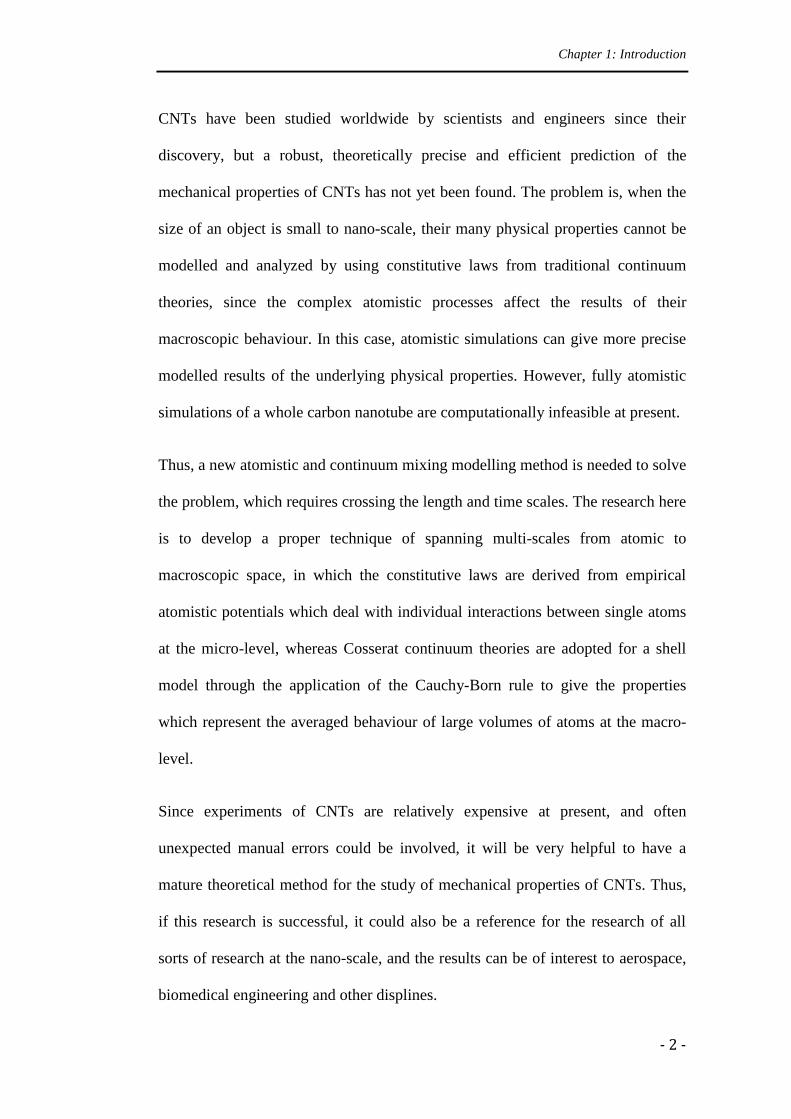
Figure 1-1: Some SWCNTs with different chiralities. (a) armchair structure (b)
zigzag structure (c) chiral structure (Dresselhaus et al. 1996) ............................... 3
Figure 1-2: Basis vectors and chiral vector ............................................................ 4
Figure 1-3: Illustration of a graphite sheet rolling to SWCNT ............................... 5
Figure 1-4: Electron micrographs of the cross section of different types of carbon
nanotube (Iijima, 1991) ........................................................................................... 6
Figure 1-5: Young’s modulus and Poisson ratio with dependence on tube
diameter. (Chang and Gao, 2003) ........................................................................... 8
Figure 1-6: Young’s modulus and shear modulus with dependence on tube
diameter. (Li and Chou, 2003) ................................................................................ 9
Figure 1-7: Young’s modulus and circular modulus with dependence on tube
diameter. (Wang et al. 2006) .................................................................................. 9
Figure 1-8: Young’s modulus and Poisson ratio with dependence on tube
diameter. (Avila and Lacerda, 2008) ...................................................................... 9
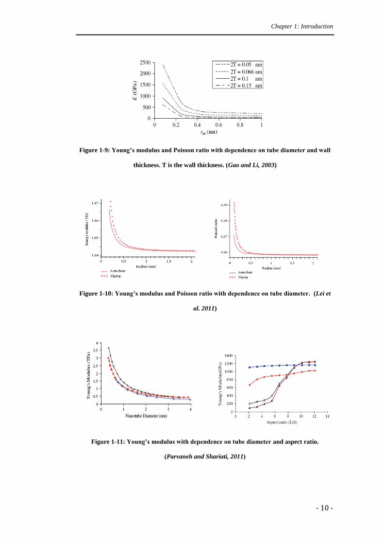
Figure 1-9: Young’s modulus and Poisson ratio with dependence on tube diameter
and wall thickness. (Gao and Li, 2003) ................................................................ 10
- ii -
Figure 1-10: Young’s modulus and Poisson ratio with dependence on tube
diameter. (Lei et al. 2011) .................................................................................... 10
Figure 1-11: Young’s modulus with dependence on tube diameter and aspect
ratio. (Parvaneh and Shariati, 2011) ................................................................... 10
Figure 1-12: Two sets of simulations of nanotube behaviour under increasing
bending strain (Huhtala et al. 2002) ..................................................................... 11
Figure 1-13: Simulation of SWCNT under axial compression (Yakobson et al.
1996)...................................................................................................................... 12
Figure 1-14: Simulation of SWCNT under torsion (Yakobson et al. 1996) ......... 12
Figure 1-15: Simulation of compressed and twisted SWCNTs (Arroyo and
Belytschko, 2004) .................................................................................................. 12
Figure 1-16: Illustration of the exponential Cauchy-Born rule (Arroyo and
Belytschko, 2003) .................................................................................................. 16
Figure 1-17: Illustration of the higher order Cauchy-Born rule (Guo et al. 2006) 19
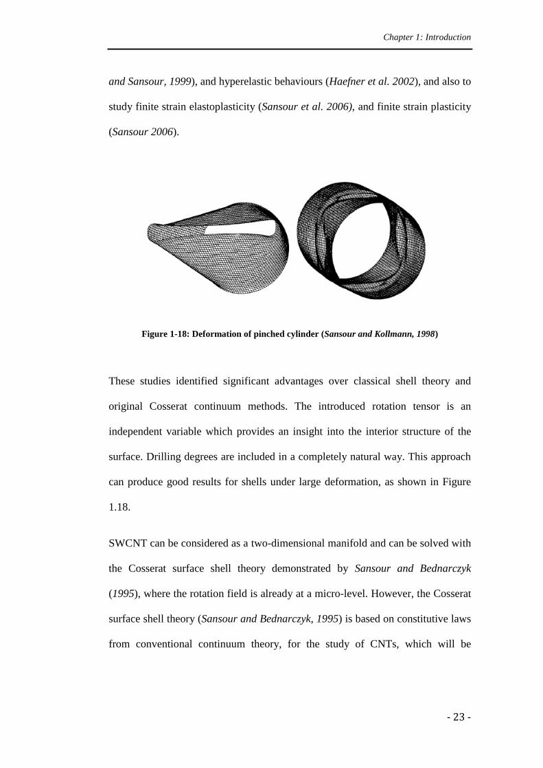
Figure 1-18: Deformation of pinched cylinder (Sansour and Kollmann, 1998) ... 23
Figure 2-1: Illustration of Cauchy-Born rule ........................................................ 32
Figure 2-2: Multi-lattice, sub-lattices, and shift vector ......................................... 34
Figure 2-3: Deformation on Cosserat surface ....................................................... 39
Figure 2-4: Opposite results in modelling critical strain of CNTs in tension by
using two generations of Brenner potential (Wu et al. 2008)................................ 48
Figure 2-5: Difference of Young’s modulus of CNTs by using two sets of
parameters in Tersoff-Brenner potential (Wang et al. 2006) ................................ 48
Figure 3-1: Sketch of 1-D atomic chain deforming in 2-D ................................... 70
Figure 3-2: Sketch of 1-D atomic chain deforming in 3-D ................................... 72
- iii -
Figure 3-3: Atomic chain model with two fixed ends under uniform load ........... 73
Figure 3-4: Deformation of atomic chain under small uniform load .................... 73
Figure 3-5: Deformation of atomic chain under large uniform load ..................... 73
Figure 3-6: Deformation of CNTs under bending (Huhtala et al. 2002) .............. 74
Figure 3-7: Cantilever atomic chain model under moment................................... 74
Figure 3-8: Deformation of atomic chain under small moment ............................ 75
Figure 3-9: Deformation of atomic chain under large moment ............................ 75
Figure 3-10: Cantilever atomic chain under uniform load .................................... 76
Figure 3-11: Cantilever atomic chain under uniform load in 3-D space ............... 77
Figure 3-12: Cantilever atomic chain under uniform load in 2-D space ............... 77
Figure 3-13: Atomic chain with two hinged ends under uniform load ................ 77
Figure 3-14: Deformation of atomic chain with two hinged ends under uniform
load in 3-D space ................................................................................................... 78
Figure 3-15: Deformation of atomic chain with two hinged ends under uniform
load in 2-D space ................................................................................................... 78
Figure 3-16: Cantilever atomic chain under moment........................................... 78
Figure 3-17: Deformation of cantilever atomic chain under moment in 3-D space
............................................................................................................................... 79
Figure 3-18: Deformation of cantilever atomic chain under moment in 2-D space
............................................................................................................................... 79
Figure 3-19: Atomic chain dynamic rod .............................................................. 80
Figure 3-20: Deformation of dynamic rod on 1-3 plane ....................................... 82
Figure 3-21: Deformation of dynamic rod on 1-2 plane ....................................... 84
Figure 3-22: Deformation of dynamic rod in isometric view ............................... 86
- iv -
Figure 3-23: Atomic chain model in torsion ......................................................... 88
Figure 3-24: A small disturbance and force to buckle .......................................... 88
Figure 3-25: Deformation of atomic chain after small disturbance ..................... 88
Figure 3-26: Simulation of atomic chain coiling up ............................................. 89
Figure 3-27: Atomistic simulation of torsion of CNT (Yakobson et al. 1996) .... 89
Figure 3-28: Transient deformations of the cross section of SWCNTs under
bending (Kutana and Giapis, 2006) ...................................................................... 91
Figure 3-29: Deformed atomic rings in simulating cross section of CNT under
bending (Vodenitcharova and Zhang, 2004)......................................................... 91
Figure 3-30: Sketch of the strategy of atomic ring in simulation of CNT in
bending .................................................................................................................. 91
Figure 3-31: Deformed atomic ring in simulating cross section of SWCNT under
bending .................................................................................................................. 92
Figure 4-1: Atom A and its first and second nearest neighbours .......................... 95
Figure 4-2: Micro-rotation on the reference plane ................................................ 96
Figure 4-3: Graphite sheet under uniform stretch loading .................................. 106
Figure 4-4: Strain and stretch loading relationship from tension method ........... 107
Figure 4-5: Graphite sheet under bending with uniform loading at the free end 108
Figure 4-6: Sketch of cylindrical shell model under tension .............................. 111
Figure 4-7: Deformation of cylindrical shell model under tension ..................... 113
Figure 4-8: Dependence of Young’s modulus on tube diameter for armchair
SWCNTs ............................................................................................................. 114
Figure 4-9: Dependence of Young’s modulus on tube diameter for zigzag
SWCNTs ............................................................................................................. 116
- v -
Figure 4-10: Dependence of Young’s modulus on tube diameter for zigzag
SWCNTs (Parvaneh and Shariati, 2011) ........................................................... 116
Figure 4-11: Comparison of Young’s modulus for armchair and zigzag SWCNTs
............................................................................................................................. 117
Figure 4-12: Comparison of Young’s modulus for armchair and zigzag SWCNTs
(Lei et al. 2011) ................................................................................................... 117
Figure 4-13: Sketch of one end fixed cylindrical shell model under bending .... 118
Figure 4-14: Deformation of one end fixed cylindrical shell under bending
(D=4.339nm; L=16nm) ....................................................................................... 118
Figure 4-15: Relationship of bending rigidity against tube diameter (one end fixed
bending) ............................................................................................................... 120
Figure 4-16: Relationship of Young’s modulus against tube diameter for
cylindrical shell mode under bending (one end fixed bending) .......................... 120
Figure 4-17: Comparison of Young’s modulus for cylindrical shell model from
tension method and bending method with different wall thickness (h) .............. 121
Figure 4-18: Young’s modulus varying with SWCNT wall thickness (2T) (Gao
and Li, 2003) ....................................................................................................... 121
Figure 4-19: Sketch of two end fixed cylindrical shell model under bending .... 122
Figure 4-20: Deformation of two end fixed cylindrical shell under bending
(D=3.390nm; L=16nm) ....................................................................................... 122
Figure 4-21: Relationship of bending rigidity against tube diameter and
comparison (two end fixed bending) ................................................................... 124
Figure 4-22: Relationship of Young’s modulus against tube diameter for
cylindrical shell mode under bending and comparison (two end fixed bending) 124
- vi -
Figure 4-23: Sketch of simply supported cylindrical shell model under bending
............................................................................................................................. 125
Figure 4-24: Deformation of two end fixed cylindrical shell under bending
(D=1.898nm; L=16nm) ....................................................................................... 125
Figure 4-25: Relationship of bending rigidity against tube diameter and
comparison .......................................................................................................... 127
Figure 4-26: Relationship of Young’s modulus against tube diameter for
cylindrical shell mode under bending and comparison (two end fixed bending) 128
Figure 4-27: Global bending and local bending of SWCNTs (Parvaneh and
Shariati, 2011) ..................................................................................................... 129
Figure 4-28: Different bending modes of SWCNTs .......................................... 129
Figure 4-29: Configurations of deflected armchair SWCNT (Yang and E, 2006)
............................................................................................................................. 130
Figure 4-30: Configurations of deflected armchair SWCNT under uniform loading
............................................................................................................................. 130
Figure 4-31: Relationship of maximum deflection and external load (Yang and E,
2006).................................................................................................................... 131
Figure 4-32: Relationship of maximum deflection and external load ................. 131
Figure 4-33: Two buckling patterns of SWCNTs under axial compression ....... 132
Figure 4-34: Simulations of buckling patterns of SWCNTs under axial
compression (Yakobson et al. 1996) ................................................................... 132
Figure 4-35: Sketch of cylindrical shell model under stretching ........................ 133
Figure 4-36: Deformation of cylindrical shell under compression (D=4.266nm;
L=8nm) ................................................................................................................ 133
- vii -
Figure 4-37: Force-strain relationship of cylindrical shell under compression with
various tube diameters ......................................................................................... 134
Figure 4-38: Critical strains of zigzag SWCNTs under compression with fixed
length ................................................................................................................... 135
Figure 4-39: Comparison of variation of critical strains with respect to tube
diameter ............................................................................................................... 135
Figure 4-40: Force-strain relationship of cylindrical shell under compression with
various tube lengths ............................................................................................. 136
Figure 4-41: Comparison of variation of critical strains with respect to aspect ratio
............................................................................................................................. 137
Figure 4-42: Deformation of cylindrical shell under compression (D=1.409nm;
L=40nm) .............................................................................................................. 138
Figure 4-43: Bending deformations of SWCNT bundle under axial compression
(Liew et al. 2006) ................................................................................................ 138
Figure 4-44: Three types of buckling modes of SWCNTs under axial compression
depending on the aspect ratios (a) results from Zhang et al. (2009) (b) present
results .................................................................................................................. 139
Figure 4-45: Sketch of cylindrical shell model under torsion ............................. 140
Figure 4-46: Deformations of cylindrical shell model under torsion .................. 140
Figure 4-47: Relationship of external torque and twisting angle ........................ 141
Figure 4-48: (a) atomistic simulation and (b) local Chauchy-Born rule result of
SWCNT under twisting (Yang and E, 2006) (c) present result ........................... 141
- viii -
Tables
Table 4-1: Comparison of Young’s modulus and tension rigidity .................... 110
Table 4-2: Dependence of Young’s modulus on tube diameter for armchair
SWCNTs ............................................................................................................. 114
Table 4-3: Dependence of Young’s modulus on tube diameter for zigzag
SWCNTs ............................................................................................................. 115
Table 4-4: Critical strains for zigzag SWCNTs with different tube diameters . 134
Table 4-5: Critical strains for zigzag SWCNTs with different aspect ratio ...... 137
- ix -
Nomenclature
undeformed lattice vector and deformed lattice vector
chiral vector
D direct derivative
D carbon nanotube diameter
permutation tensor (Levi-Civita tensor) (i, j, k = 1, 2, 3)
Cartesian co-ordinates (i = 1, 2, 3)
E Young’s modulus
external forces on the surface and on the boundary
F applied force
deformation gradient
covariant base vectors of and
Riemannian metric
h carbon nanotube effective wall thickness
axial vector of
l axial vector of L
- x -
L right multiplication of rotation tensor
tensor-like bending modulus
tensor-like stretch modulus
normal vector
external torques on the surface and on the boundary
rotation tensor
area of representative atomic cell
force tensor
couple tensor
displacement vector
first Cosserat deformation tensor
interatomic potential
strain energy density
a point on reference configuration and its position after
deformation
reference and deformed surface
strain
Ricci tensor
co-ordinates in ,
second Cosserat deformation tensor
eigenvector of
inner displacement vector
Chapter 1: Introduction
- 1 -
Chapter 1
Introduction
1.1 Background
It was a revolution in nano-science when carbon nanotubes (CNTs) were
discovered by Iijima in 1991 with their outstanding properties. Because of their
unique electrical properties and extremely high thermal conductivity, CNTs have
been used for electronics, field-emission displays, energy storage, functional
fillers in composites, and some biomedical devices (Ajayan and Zhou 2001;
Baughman et al. 2002; Endo et al. 2006). Moreover, CNTs have high elastic
modulus (>1TPa), large elastic strain - up to 5%, and large breaking strain - up to
20% (Iijima 1991). Their excellent mechanical properties could lead to many
more applications. For example, with their amazing strength and stiffness, plus the
advantage of lightness, perspective future applications of CNTs are in aerospace
engineering and virtual bio-devices.
Chapter 1: Introduction
- 2 -
CNTs have been studied worldwide by scientists and engineers since their
discovery, but a robust, theoretically precise and efficient prediction of the
mechanical properties of CNTs has not yet been found. The problem is, when the
size of an object is small to nano-scale, their many physical properties cannot be
modelled and analyzed by using constitutive laws from traditional continuum
theories, since the complex atomistic processes affect the results of their
macroscopic behaviour. In this case, atomistic simulations can give more precise
modelled results of the underlying physical properties. However, fully atomistic
simulations of a whole carbon nanotube are computationally infeasible at present.
Thus, a new atomistic and continuum mixing modelling method is needed to solve
the problem, which requires crossing the length and time scales. The research here
is to develop a proper technique of spanning multi-scales from atomic to
macroscopic space, in which the constitutive laws are derived from empirical
atomistic potentials which deal with individual interactions between single atoms
at the micro-level, whereas Cosserat continuum theories are adopted for a shell
model through the application of the Cauchy-Born rule to give the properties
which represent the averaged behaviour of large volumes of atoms at the macro-
level.
Since experiments of CNTs are relatively expensive at present, and often
unexpected manual errors could be involved, it will be very helpful to have a
mature theoretical method for the study of mechanical properties of CNTs. Thus,
if this research is successful, it could also be a reference for the research of all
sorts of research at the nano-scale, and the results can be of interest to aerospace,
biomedical engineering and other displines.
Chapter 1: Introduction
- 3 -
1.2 Structure of carbon nanotubes
Carbon nanotubes (CNTs) are tubular carbon molecules with particular properties.
Generally, they can be divided in two main categories: single-walled carbon
nanotubes (SWCNTs) and multi-walled carbon nanotubes (MWCNTs). SWCNTs
can be considered as rectangular strips of hexagonal graphite monolayers rolling
up to cylinder tubes. Two types of SWCNTs with high symmetry are normally
selected by researchers, which are zigzag SWCNTs and armchair SWCNTs.
When some of the atomic bonds are parallel to the tube axis, the CNT is called a
zigzag CNT, while if the bonds are perpendicular to the axis, it is called an
armchair CNT, and for any other structures, they are called chiral CNTs, as shown
in Figure 1.1 (Dresselhaus et al. 1996).
Figure 1-1: Some SWCNTs with different chiralities. (a) armchair structure (b) zigzag
structure (c) chiral structure (Dresselhaus et al. 1996)
Chapter 1: Introduction
- 4 -
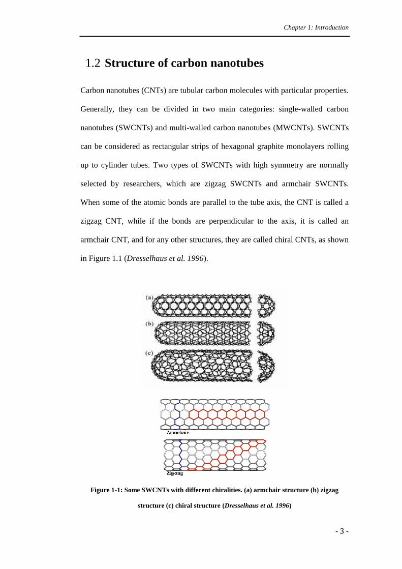
Figure 1-2: Basis vectors and chiral vector
Chiral vector is a vector that maps an atom of one end of the tube to the other.
can be an integer multiple of and , which are two basis vectors of the
graphite cell. Then we have , with integer and , and the
constructed CNT is called a CNT, as shown in Figure 1.2. It can be proved
that for armchair CNTs , and for zigzag CNTs . For example, in
Figure 1.2, the structure is designed to be a (4,0) zigzag SWCNT.
MWCNT can be considered as the structure of a bundle of concentric SWCNTs
with different diameters. The length and diameter of MWCNTs are different from
those of SWCNTs, which means, of course, their properties differ significantly.
This research concentrates on solving the mechanical properties of SWCNTs. In
further research, MWCNTs can be modelled as a collection of SWCNTs, provided
the interlayer interactions are modelled by Van der Waals forces in the simulation.
Chapter 1: Introduction
- 5 -
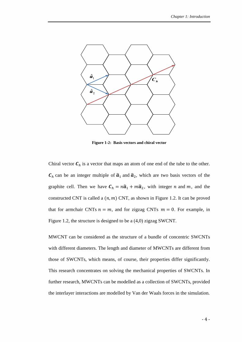
A SWCNT can be modelled as a hollow cylinder by rolling a graphite sheet as
shown in Figure 1.3. If a planar graphite sheet is considered to be an undeformed
configuration, and the SWCNT is defined as the current configuration, then the
relationship between the SWCNT and the graphite sheet can be shown to be:
where are the material co-ordinates of a point in the initial configuration
and and are the co-ordinates in the current configuration. R is the radius
of the modelled SWCNT. The relationship between the integers and the
radius of SWCNT is given by , where ,
and is the length of a non-stretched C-C bond which is given by Wu
et al. (2006).
Figure 1-3: Illustration of a graphite sheet rolling to SWCNT
As a graphite sheet can be ‘rolled’ into a SWCNT, we can ‘unroll’ the SWCNT to
a plane graphite sheet. Since a SWCNT can be considered as a rectangular strip of
hexagonal graphite monolayer rolling up to a cylindrical tube, the general idea is
that it can be modelled as a cylindrical shell, a cylinder surface, or it can pull-back
Chapter 1: Introduction
- 6 -
to be modelled as a plane sheet deforming into curved surface in three-
dimensional space. A MWCNT can be modelled as a combination of a series of
concentric SWCNTs with inter-layer interatomic reactions.
Provided the continuum shell theory captures the deformation at the macro-level,
the inner micro-structure can be described by finding the appropriate form of the
potential function which is related to the position of the atoms at the atomistic
level. Therefore, the SWCNT can be considered as a generalized continuum with
microstructure.
1.3 Literature Review
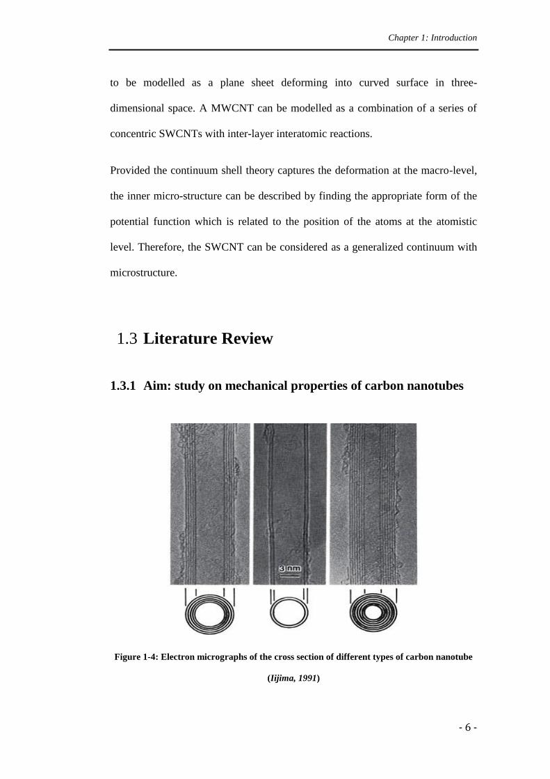
1.3.1 Aim: study on mechanical properties of carbon nanotubes
Figure 1-4: Electron micrographs of the cross section of different types of carbon nanotube
(Iijima, 1991)
Chapter 1: Introduction
- 7 -
Since the discovery of CNTs, their mechanical properties have been the subject of
many studies. Generally, CNTs can be divided into two types: single-walled
(SWCNTs) and multi-walled carbon nanotubes (MWCNTs). A transmission
electron micrograph of different types of carbon nanotube is shown in Figure 1.4.
1.3.1.1 Young’s modulus
Young’s modulus and Poisson ratio are two independent elastic constants which
are important measures of stiffness in classical elasticity theory. However, the
established definitions of elastic measures in solid mechanics may fail in CNTs,
since the spacing and the inner structure are very complex at the nano-scale.
Iijima (1991) obtained Young’s modulus of CNTs around 1TPa. Treacy et al.
(1996) observed a much higher Young’s modulus of CNTs to an axial load. A
large scatter in the value of Young’s modulus for CNTs exists, whether in
experimental results or in theoretical calculations, which varies from 0.5TPa to
6TPa. In addition, researchers also presented different points of view on how the
scale of tube diameter affects Young’s modulus of CNTs.
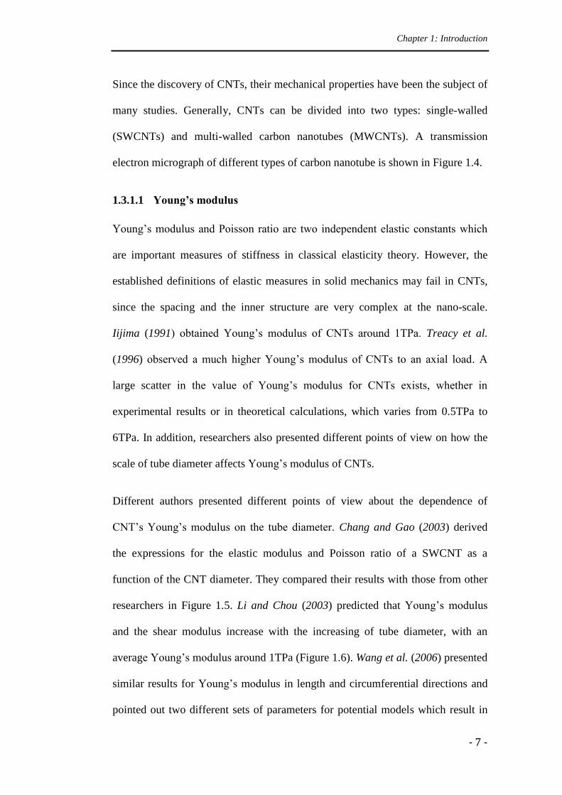
Different authors presented different points of view about the dependence of
CNT’s Young’s modulus on the tube diameter. Chang and Gao (2003) derived
the expressions for the elastic modulus and Poisson ratio of a SWCNT as a
function of the CNT diameter. They compared their results with those from other
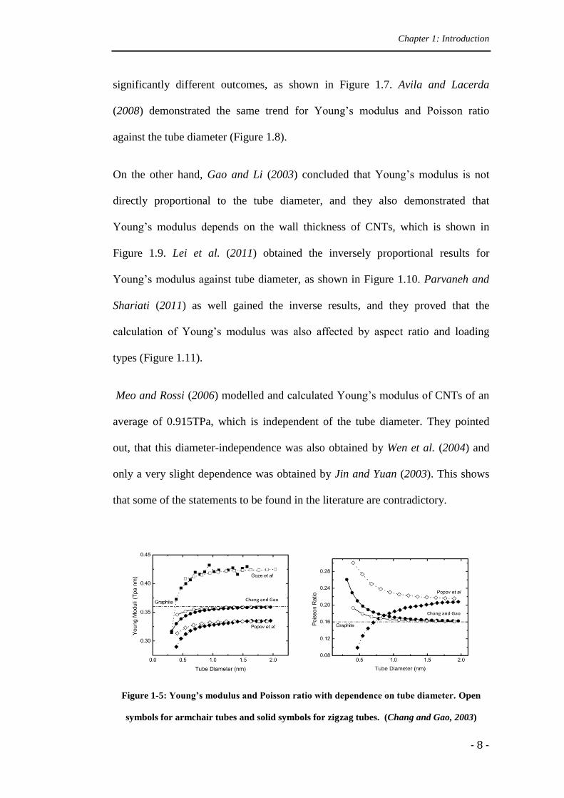
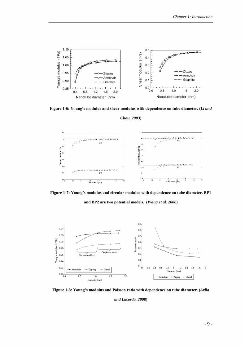
researchers in Figure 1.5. Li and Chou (2003) predicted that Young’s modulus
and the shear modulus increase with the increasing of tube diameter, with an
average Young’s modulus around 1TPa (Figure 1.6). Wang et al. (2006) presented
similar results for Young’s modulus in length and circumferential directions and
pointed out two different sets of parameters for potential models which result in
Chapter 1: Introduction
- 8 -
significantly different outcomes, as shown in Figure 1.7. Avila and Lacerda
(2008) demonstrated the same trend for Young’s modulus and Poisson ratio
against the tube diameter (Figure 1.8).
On the other hand, Gao and Li (2003) concluded that Young’s modulus is not
directly proportional to the tube diameter, and they also demonstrated that
Young’s modulus depends on the wall thickness of CNTs, which is shown in
Figure 1.9. Lei et al. (2011) obtained the inversely proportional results for
Young’s modulus against tube diameter, as shown in Figure 1.10. Parvaneh and
Shariati (2011) as well gained the inverse results, and they proved that the
calculation of Young’s modulus was also affected by aspect ratio and loading
types (Figure 1.11).
Meo and Rossi (2006) modelled and calculated Young’s modulus of CNTs of an
average of 0.915TPa, which is independent of the tube diameter. They pointed
out, that this diameter-independence was also obtained by Wen et al. (2004) and
only a very slight dependence was obtained by Jin and Yuan (2003). This shows
that some of the statements to be found in the literature are contradictory.
Figure 1-5: Young’s modulus and Poisson ratio with dependence on tube diameter. Open
symbols for armchair tubes and solid symbols for zigzag tubes. (Chang and Gao, 2003)
Chapter 1: Introduction
- 9 -
Figure 1-6: Young’s modulus and shear modulus with dependence on tube diameter. (Li and
Chou, 2003)
Figure 1-7: Young’s modulus and circular modulus with dependence on tube diameter. BP1
and BP2 are two potential models. (Wang et al. 2006)
Figure 1-8: Young’s modulus and Poisson ratio with dependence on tube diameter. (Avila
and Lacerda, 2008)
Chapter 1: Introduction
- 10 -
Figure 1-9: Young’s modulus and Poisson ratio with dependence on tube diameter and wall
thickness. T is the wall thickness. (Gao and Li, 2003)
Figure 1-10: Young’s modulus and Poisson ratio with dependence on tube diameter. (Lei et
al. 2011)
Figure 1-11: Young’s modulus with dependence on tube diameter and aspect ratio.
(Parvaneh and Shariati, 2011)
Chapter 1: Introduction
- 11 -
1.3.1.2 Bending, buckling and torsion
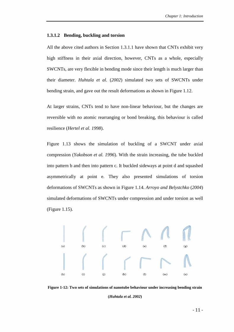
All the above cited authors in Section 1.3.1.1 have shown that CNTs exhibit very
high stiffness in their axial direction, however, CNTs as a whole, especially
SWCNTs, are very flexible in bending mode since their length is much larger than
their diameter. Huhtala et al. (2002) simulated two sets of SWCNTs under
bending strain, and gave out the result deformations as shown in Figure 1.12.
At larger strains, CNTs tend to have non-linear behaviour, but the changes are
reversible with no atomic rearranging or bond breaking, this behaviour is called
resilience (Hertel et al. 1998).
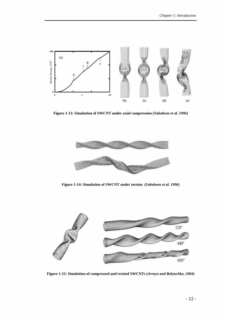
Figure 1.13 shows the simulation of buckling of a SWCNT under axial
compression (Yakobson et al. 1996). With the strain increasing, the tube buckled
into pattern b and then into pattern c. It buckled sideways at point d and squashed
asymmetrically at point e. They also presented simulations of torsion
deformations of SWCNTs as shown in Figure 1.14. Arroyo and Belystchko (2004)
simulated deformations of SWCNTs under compression and under torsion as well
(Figure 1.15).
Figure 1-12: Two sets of simulations of nanotube behaviour under increasing bending strain
(Huhtala et al. 2002)
Chapter 1: Introduction
- 12 -
Figure 1-13: Simulation of SWCNT under axial compression (Yakobson et al. 1996)
Figure 1-14: Simulation of SWCNT under torsion (Yakobson et al. 1996)
Figure 1-15: Simulation of compressed and twisted SWCNTs (Arroyo and Belytschko, 2004)
Chapter 1: Introduction
- 13 -
1.3.2 Inspirations on methodologies
1.3.2.1 Nanomechanics
Traditional continuum mechanics have been used to model CNTs in early years.
Govindjee and Sackman (1999) used a simple Bernoulli–Euler beam model and
continuum elastic theory to calculate the Young’s Modulus of CNTs. Pantano et
al. (2004) built CNT models with shell theory using continuum methods as well.
Natsuki and Endo (2004) also simulated mechanical properties of CNTs based on
a continuum shell model. Afterwards continuum cylindrical shell models were
widely applied in the buckling analysis of CNTs (He et al. 2005, Zhang et al.
2006, Yang and Wang 2007). But, as shown by Govindjee and Sackman (1999),
the mechanical properties of CNTs are distinctly dependent on the size of the
system, thus in nano-scale situations, the constitutive laws of traditional
continuum mechanics are no longer applicable. Wang et al. (2006) also proved the
dependence on scale effect in studying CNTs. They observed that solutions
obtained from classical elastic beam and shell model were significantly
overestimated, so the scale effect had to be taken into account to provide
reasonable results.
The more accurate modelling of CNTs is via atomistic methods, which considers
each atom as its fundamental unit and describes their behaviour by a series of
equations. One of the most popular atomistic models of CNTs is the empirical
potential molecular mechanics model, which considers a series of atoms as
repeating units and predicts the potential energies as a function of the positions of
atoms. Bao et al. (2004) studied Young’s moduli of CNTs based on molecular
Chapter 1: Introduction
- 14 -
dynamics (MD) simulation. Chang and Gao (2003) also presented the elastic
properties of SWCNTs through a molecular mechanics approach, and
recommended further applications of molecular mechanics in CNTs modelling.
Liew et al. (2004) also used MD simulations to describe the mechanical properties
of CNTs. In addition to the elastic properties, such as Young’s modulus and
Poisson’s ratio, they studied the plastic behaviour and the fracture of CNTs. Sun
and Zhao (2005) used a finite element model based on molecular mechanics to
calculate the strength of SWCNTs. Meo and Rossi (2006) applied molecular
mechanics based finite element approach to simulate the fracture progress in
CNTs.
Atomistic simulation is necessary for the fracture study of CNTs, because
continuum mechanics cannot capture all the details of an atomic bond breakage or
dislocation at a micro-level (Belytschko et al. 2002, Lu and Bhattacharya 2005,
Meo and Rossi 2006). Since this research is concentrating on the study of the
elastic properties of CNTs, there is no need for a full atomistic simulation of a
whole CNT which would be extremely computationally expensive and time
consuming rendering it impractical. Therefore, a new atomistic and continuum
mixing method needs to be established, which is computationally practical and
can provide more accurate physical results than a classical continuum theory.
To apply continuum mechanics to the study of CNTs, the first step is to think
about how to link the continuum behaviour of CNTs with the atomic deformations
at the nano-level. In this aspect, the inspiration came from Arroyo and Belytschko
(2003, 2004) with the idea of applying modified Cauchy-Born rule on the study of
mechanical properties of CNTs.
Chapter 1: Introduction
- 15 -
1.3.2.2 The Cauchy-Born rule
The Cauchy-Born rule is a rule to link the atomistic field to the continuum world
that describes the relations between the deformation of atom lattice vectors and
the deformation of bulk vectors. As pointed out by Arroyo and Belytschko (2003,
2004), the Cauchy–Born rule is not directly suitable to applications of CNT,
because CNT can be viewed as a curved surface, and the deformation gradient
maps the deformed vector on the tangent space of the deformed curve instead of
the real chord vector which lies on the curve. In order to achieve more accurate
results through Cauchy-Born rule, different kinds of modifications have been
created. Arroyo and Belytschko (2003, 2004) developed a so-called exponential
Cauchy-Born rule which was demonstrated naturally mapping the tangent vector
into the chord on the curved surface. Guo et al. (2006) presented a higher order
Cauchy-Born rule by preserving more higher-order terms in Taylor’s expansion to
improve the accuracy of approximation. Since modification of the Cauchy-Born
rule is an important inspiration of this research, the exponential and higher order
Cauchy-Born rules are briefly explained.
1.3.2.2.1 Exponential Cauchy-Born rule
Arroyo and Belytschko (2003, 2004) described two-dimensional manifold
deforming in three-dimensional Euclidean space. The undeformed surface
represents the planar grapheme as the reference configuration. It is
changed by the deformation map into the deformed surface . The
deformation gradient is the tangent of the configuration map , which maps
infinitesimal vectors of the undeformed plane into vectors on the tangent plane
of the deformed surface (Figure 1.16). The standard Cauchy-Born rule
Chapter 1: Introduction
- 16 -
produces vectors after deformation map on the tangent plane of the deformed
surface instead of the real chord on the curve of the surface. In order to capture the
effect of curvature in the deformed surface, Arroyo and Belytschko (2003, 2004)
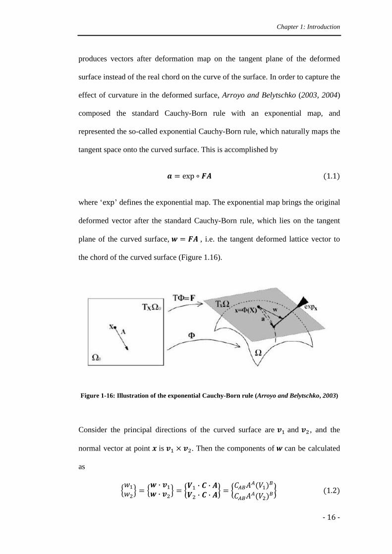
composed the standard Cauchy-Born rule with an exponential map, and
represented the so-called exponential Cauchy-Born rule, which naturally maps the
tangent space onto the curved surface. This is accomplished by
where ‘ ’ defines the exponential map. The exponential map brings the original
deformed vector after the standard Cauchy-Born rule, which lies on the tangent
plane of the curved surface, , i.e. the tangent deformed lattice vector to
the chord of the curved surface (Figure 1.16).
Figure 1-16: Illustration of the exponential Cauchy-Born rule (Arroyo and Belytschko, 2003)
Consider the principal directions of the curved surface are and , and the
normal vector at point is . Then the components of can be calculated
as
Chapter 1: Introduction
- 17 -
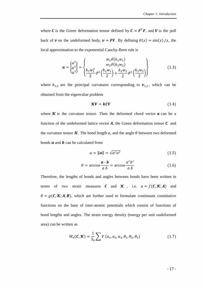
where is the Green deformation tensor defined by , and is the pull
back of on the undeformed body, . By defining , the
local approximation to the exponential Cauchy-Born rule is
where are the principal curvatures corresponding to , which can be
obtained from the eigenvalue problem
where is the curvature tensor. Then the deformed chord vector can be a
function of the undeformed lattice vector , the Green deformation tensor and
the curvature tensor . The bond length , and the angle between two deformed
bonds and can be calculated from
Therefore, the lengths of bonds and angles between bonds have been written in
terms of two strain measures and , i.e. and
, which are further used to formulate continuum constitutive
functions on the base of inter-atomic potentials which consist of functions of
bond lengths and angles. The strain energy density (energy per unit undeformed
area) can be written as

Chapter 1: Introduction
- 18 -
defines the area of a unit cell, are the bond lengths of the three bonds
connected on one atom, are the bond angles between the three bonds.
Two stress measures, a force stress tensor, where is the second Piola-Kirchhoff
stress tensor, and a moment like stress tensor , can be derived from
Lagrangian elasticity tensors can be obtained by second derivatives
These three tensors represent in-plane stiffness, bending stiffness and coupling
stiffness respectively (Arroyo and Belytschko, 2002,2003,2004). It is written
instead of due to the consideration of inner displacement functioning in the
potential form, which will be further explained in Section 2.3.2.
1.3.2.2.2 Higher order Cauchy-Born rule
Guo et al. (2006) presented an extension of the standard Cauchy-Born rule by
introducing a higher order deformation gradient. In classical continuum
mechanics deformation gradient is defined by
Instead of the standard Cauchy-Born rule , Leamy et al. (2003) defined
the deformed lattice vector as
is assumed to be a Taylor’s expansion of the deformation field
Chapter 1: Introduction
- 19 -
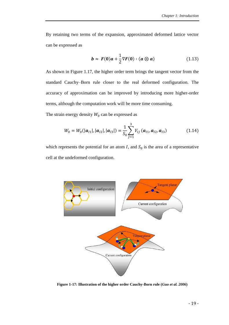
By retaining two terms of the expansion, approximated deformed lattice vector
can be expressed as
As shown in Figure 1.17, the higher order term brings the tangent vector from the
standard Cauchy–Born rule closer to the real deformed configuration. The
accuracy of approximation can be improved by introducing more higher-order
terms, although the computation work will be more time consuming.
The strain energy density can be expressed as
which represents the potential for an atom , and is the area of a representative
cell at the undeformed configuration.
Figure 1-17: Illustration of the higher order Cauchy-Born rule (Guo et al. 2006)
Chapter 1: Introduction
- 20 -
where and denote the deformed and undeformed lattice vectors. The
following relations hold
with which the strain energy density can be written as
The first Piola-Kirchhoff stress tensor and the higher-order stress tensor are
where is the generalized force defined as
Let , where
is taken as the form of interatomic potential for carbon.
The generalized stiffness is defined as
The modulus tensors can be derived as
Chapter 1: Introduction
- 21 -
Again it is written instead of because of the inclusion of inner
displacement in potential functions.
Both the above methods are based on the same idea by adding extra higher order
terms into the deformation gradient in order to approximate the real curve after
standard Cauchy-Born rule, which is different in this research where the standard
Cauchy-Born rule stays to describe the strain at the tangent plane, and
modification is made by adding a displacement field-independent rotation tensor
at each point of the surface, which describes the curvature by rotating the
deformed vector on the tangent plane into the real deformed curve itself. Thus, the
Cosserat continuum theory is introduced via the independent rotation tensor in
order to describe the curvature of the deformed surface after applying the standard
Cauchy-Born rule to the tangent vectors. Cosserat surface as a shell model is
established in this research since SWCNT can be modelled as a hollow cylindrical
shell, therefore built as a two-dimensional surface instead of a three-dimensional
solid continuum.
1.3.2.3 Cosserat surface as a shell model
SWCNTs, as well MWCNTs have been modelled as linear elastic shells (Tu and
Ou-yang, 2002, Pantano et al. 2004) or non-linear elastic shells (Arroyo and
Belytschko, 2002,2003,2004) via continuum mechanics methods. In the linear
elastic range, Young’s modulus and the wall thickness were found by fitting the
interatomic model, covering a large range from 0.5TPa to 6TPa, and from 0.06nm
to 0.6 nm.
Chapter 1: Introduction
- 22 -
Wu et al. (2008) developed a finite-deformation shell theory for CNTs based on
the interatomic potentials for carbon. Shell theory based on interatomic potentials
is the approach by all the authors above and as well as in this research. Wu et al.
(2008) set a relationship for the rates of the second Piola-Kirchhoff stress tensor
and the bending moment tensor to the increments of Green strain tensor and
curvature tensor as
where , and , are the tension, bending and coupling rigidity derived
from interatomic potentials
and it modified the constitutive model in classical continuum shell theory by
adding extra coupling terms to describe the stress-curvature and moment-strain
relations.
Sansour and Bednarczyk (1995) presented a shell theory for the Cosserat surface
which is considered as a two-dimensional manifold in Cosserat continuum, and
the surface is attached with a determined displacement field and an independent
rotation field. In classical continuum mechanics elasticity theory there are two
elastic constants involved which can be directly derived from the displacement
field, but Cosserat continuum theory introduces one more material constant that is
related to a three parametric rotation tensor attached to every particle of the
continuum, which takes into consideration size effects in the calculations. The
theory has been developed in further years to model viscoplastic shells (Kollman
Chapter 1: Introduction
- 23 -
and Sansour, 1999), and hyperelastic behaviours (Haefner et al. 2002), and also to
study finite strain elastoplasticity (Sansour et al. 2006), and finite strain plasticity
(Sansour 2006).
Figure 1-18: Deformation of pinched cylinder (Sansour and Kollmann, 1998)
These studies identified significant advantages over classical shell theory and
original Cosserat continuum methods. The introduced rotation tensor is an
independent variable which provides an insight into the interior structure of the
surface. Drilling degrees are included in a completely natural way. This approach
can produce good results for shells under large deformation, as shown in Figure
1.18.
SWCNT can be considered as a two-dimensional manifold and can be solved with
the Cosserat surface shell theory demonstrated by Sansour and Bednarczyk
(1995), where the rotation field is already at a micro-level. However, the Cosserat
surface shell theory (Sansour and Bednarczyk, 1995) is based on constitutive laws
from conventional continuum theory, for the study of CNTs, which will be
Chapter 1: Introduction
- 24 -
deviated in this research by constitutive laws derived from empirical interatomic
potentials which describe the real interactions among atoms at an atomic level.
1.4 Outline
This research is to propose a new multi-scale modelling method to simulate the
mechanical properties of SWCNTs. The central idea of the method is to consider
SWCNT as a Cosserat surface based on continuum shell theory. Constitutive laws
are derived from empirical interatomic potential functions which describe the
local potential of CNTs at the atomic level. The Cauchy-Born rule is applied to
connect the atomic description to a macroscopic space, which provides the strain
changing on the deformed surface. A shift vector is needed for the hexagonal
arrangement of atoms in SWCNT. An independent rotation tensor is employed to
compute the change of curvature of the deformed surface which is introduced in
Cosserat surface shell theory to overcome the application of the standard Cauchy-
Born rule on the study of CNTs. The Cosserat surface shell model is then
analyzed to produce results and simulations through a finite element approach.
Chapter 1 has given the background of CNTs and the previous studies of CNTs.
The literature review mainly includes research results of the linear and non-linear
elastic properties of CNTs from previous researchers, and discusses the
methodologies for studying SWCNTs. From inadequate continuum mechanics to
computationally difficult atomistic simulations, we are looking for a decent
approach to link them and give more accurate results of CNTs in a practical way.
Chapter 2 presents the whole methodologies. Section 2.1 shows the main structure
of the modelling methods. Section 2.2 explains the Cauchy-Born rule and why it
Chapter 1: Introduction
- 25 -
should be modified when studying CNTs. This section also introduces a shift
vector which should be taken into account when the Cauchy-Born rule is applied
to a non-centrosymmetric structure. Section 2.3 presents a shell theory for
Cosserat surface, in which the deformation gradient, the rotation tensor and the
strain measures are defined, and where the equilibrium equations are derived from
the principle of virtual work. Section 2.4 provides the potential forms designed for
the one-dimensional rod and two-dimensional surface to be applied in the next
two chapters. Section 2.5 provides the implementation of finite element approach
based on shell theory of the Cosserat surface. The finite element formulation is
developed, and an updating method of the rotation tensor is designed so as to be
path independent.
Chapter 3 designs an atomic chain model, and simulates the deformations from
one-dimensional to two-dimensional and to three-dimensional space. Numerical
modelling equations are given. Results are presented and compared. Simulations
of a one-dimensional embedded rod, a thread in torsion and a cross section of
CNTs in bending are demonstrated. It shows that atomic chains and CNTs have
many behaviours in common. Although the quantitative physical meaning of
atomic chain is still under development, it gives a fundamental preparation of full
graphite sheet and CNT simulations.
Chapter 4 further demonstrates the Cosserat surface as a shell model which is
applied to a two-dimensional graphite sheet deforming in-plane and out-of-plane.
Young’s modulus and Poisson ratio are predicted for the graphite sheet and the
results are compared with the literature. SWCNTs are modelled as cylindrical
shells, and deformations of SWCNTs under bending, compression and torsion are
Chapter 1: Introduction
- 26 -
simulated. Young’s modulus is predicted from cylindrical shell bending models.
Buckling strains are predicted from force-strain relationship figures for cylindrical
shell model under compression. A twisting angle against external torque force
relationship is shown for the cylindrical shell model under torsion.
Chapter 5 summarises and concludes the work carried out in this research.
Discussions about the modelling methods and the results are presented. Possible
improvements are suggested towards the end of the chapter.
Chapter 1: Introduction
- 27 -
Chapter 2
Modelling Methods
2.1 Main Idea
The aim of this research is to study the mechanical properties of SWCNTs. Two
kinds of methodologies have been established by other researchers, one being
continuum mechanics-based, and the other by atomistic simulations.
Traditional continuum mechanics have been used to model CNTs in earlier years.
Two main approaches are based on the Bernoulli–Euler beam model and the
continuum cylindrical shell model. However, as for the study of the mechanical
properties of CNTs many of the assumptions in classical continuum mechanics
are no longer applicable because of the size effect of nano-structures. Wang et al.
(2006) pointed out that the classical elastic beam and shell models provided
highly overestimated results when modelling CNTs, thus, the scale effect cannot
Chapter 2: Modelling Methods
- 28 -
be ignored, although atomistic simulations give accurate results when modelling
CNTs, the very fact that one has to calculate every atom in the system makes them
incredibly time consuming and computationally inefficient. Therefore, a bridge
linking continuum mechanics and atomistic simulations is developed.
The Cauchy-Born rule is a rule to relate the deformation of an atom bond vector at
a micro-level to the deformation of the bulk vector at a macro-level. It is
applicable for solid crystals, but it is not suitable to apply to CNTs, because the
map Cauchy-Born builds leads to a deformed vector lying on the tangent plane of
the curved surface instead of lying on the curve. However motivated by the
exponential Cauchy-Born rule (Arroyo and Belytschko 2002) and the higher order
Cauchy-Born rule (Guo et al. 2006), a modification of the standard Cauchy-Born
to applications for modelling CNTs as shells is established.
In this research an alternative way is investigated. A shell theory based on
Cosserat continua is presented to model CNTs following the work of Sansour and
Bednarczyk (1995). A displacement field-independent rotation tensor is
introduced to describe the micro-level rotation, which also makes up for the
shortcomings of the standard Cauchy-Born rule, and can take size-effects into
account. The main idea of this research is to consider SWCNT as a two-
dimensional manifold and solving it with the Cosserat surface shell theory as
demonstrated. The deformation can be described by a stretch tensor and a rotation
tensor. Responding to external force, the surface deforms providing a force stress
field and a couple stress field. A force stress tensor can be obtained from the first
derivative of the potential with respect to a stretch tensor, and a couple stress
tensor can be obtained from the first derivative of the potential with respect to a
Chapter 2: Modelling Methods
- 29 -
curvature tensor. Stretch modulus tensors can be found from the second derivative
of the potential with respect to the stretch tensor, and bending modulus tensor can
be calculated from the second derivative of potential with respect to the curvature
tensor. In order to solve for these four fields mentioned above, a way to describe
the material mechanical properties, one needs to identify the right potential forms
that are adequate at an atomistic level and applicable for continuum formulations.
Two sets of models are considered in this research. As a hypothetical example,
also being the preparation of the whole CNT modelling, an atomic chain model,
referred to as a Cosserat curve, is developed as a one-dimensional rod deforming
in a three-dimensional space. Further modelling is carried out by considering
SWCNT as a Cosserat surface deforming in a three-dimensional space. For the
atomic chain model, the energy functions are chosen from molecular mechanics,
which is also called the force field method. The total energy is determined by the
interactions of the atoms, which takes into account contributions from atom bond
stretching, bending between atom bonds and torsion energy. This model can be
considered as an atomic chain that consists of a series of carbon atoms, and C-C
bonds, which deforms in an atomic field.
For two-dimensional Cosserat surface of the SWCNT model, empirical functions
of potentials are adopted which are practical and appropriate to describe the total
potential of CNTs relatively accurately. The simplest potential functions, for
example the Morse potential, have no dependence on the environment of the
atoms, therefore not suitable to apply to a Cosserat surface. Thus we have to go
for relatively complicated potentials which incorporate the effects of atom bond
angles and bond orders, among which the Tersoff and Brenner potential (Tersoff,
Chapter 2: Modelling Methods
- 30 -
1988, Brenner, 1989) involves the variations of bond energy due to changes in the
position of an atom and also its neighbour atoms. A first generation of Tersoff and
Brenner potentials was extensively applied in the study CNTs (Belytschko et al.
2002, Zhang et al. 2002, Bao et al. 2004, Liew et al. 2004). Brenner et al. (2002)
made a few adjustments and developed a second generation of Brenner potentials,
which they claimed to be more accurate to model the real interactomic reactions.
The finite element formulation is developed on the basis of variational principles.
The stress fields and the modulus fields can thus be calculated via iteration
procedures by updating displacement fields and rotation fields, where the rotation
fields are designed to be path-independent in updating.
Section 2.2 demonstrates the Cauchy-Born rule, and also explains how the
Cauchy-Born rule links continuum systems with the atomistic world, and why it
should be modified to study surfaces when modelling CNTs. Also, an inner shift
vector is introduced due to the restrictions of the Cauchy-Born rule when applied
to the hexagonal structure of carbon cells. Section 2.3 presents the shell theory of
the Cosserat surface, where a displacement field-independent rotation tensor is
introduced, which is applied in this research instead of the modified Cauchy-Born
rule, by rotating the tangent vector which is on the tangent plane of deformed
surface into the real curve which lies on the deformed surface. Section 2.4 aims to
find the appropriate forms of the potential functions to describe the potential of
the atomic chain and the potential of a graphite sheet which is also used as a
potential for CNTs. Section 2.5 furnishes the implementation of finite element
approach of the Cosserat surface.
Chapter 2: Modelling Methods
- 31 -
2.2 Cauchy-Born rule
2.2.1 Standard Cauchy-Born rule
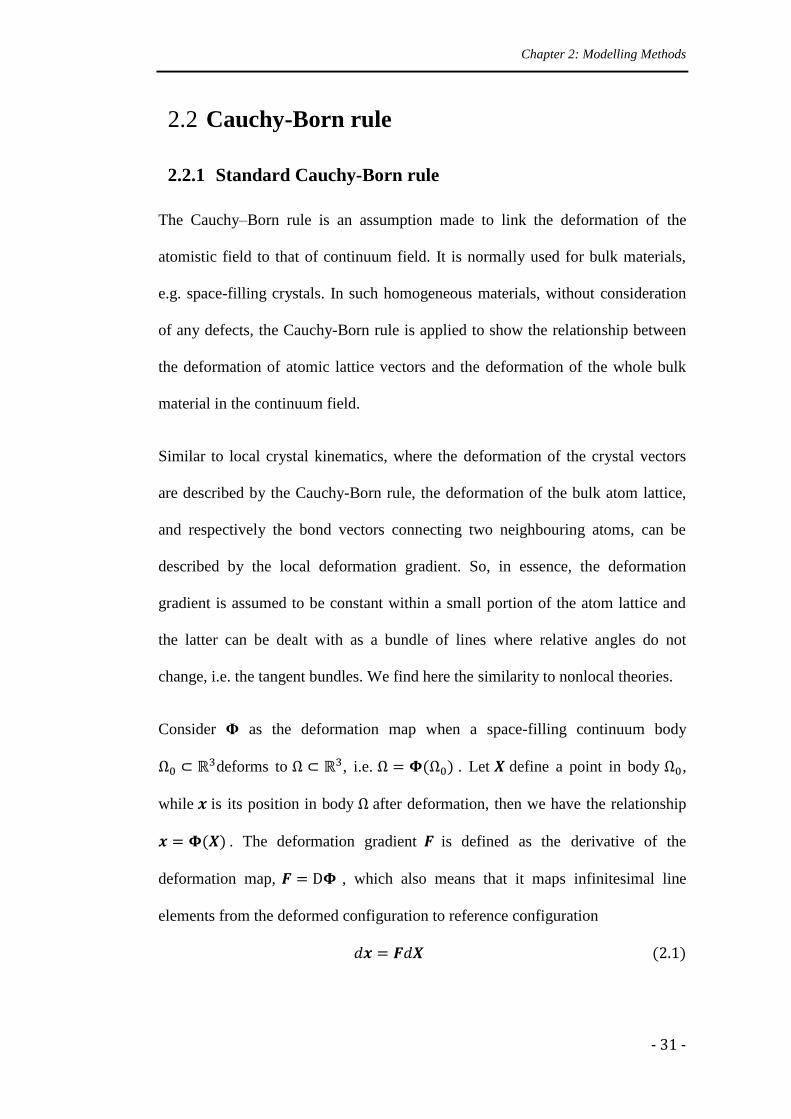
The Cauchy–Born rule is an assumption made to link the deformation of the
atomistic field to that of continuum field. It is normally used for bulk materials,
e.g. space-filling crystals. In such homogeneous materials, without consideration
of any defects, the Cauchy-Born rule is applied to show the relationship between
the deformation of atomic lattice vectors and the deformation of the whole bulk
material in the continuum field.
Similar to local crystal kinematics, where the deformation of the crystal vectors
are described by the Cauchy-Born rule, the deformation of the bulk atom lattice,
and respectively the bond vectors connecting two neighbouring atoms, can be
described by the local deformation gradient. So, in essence, the deformation
gradient is assumed to be constant within a small portion of the atom lattice and
the latter can be dealt with as a bundle of lines where relative angles do not
change, i.e. the tangent bundles. We find here the similarity to nonlocal theories.
Consider Φ as the deformation map when a space-filling continuum body
deforms to , i.e. . Let define a point in body ,
while is its position in body after deformation, then we have the relationship
. The deformation gradient is defined as the derivative of the
deformation map, , which also means that it maps infinitesimal line
elements from the deformed configuration to reference configuration
Chapter 2: Modelling Methods
- 32 -
In elasticity theory, under finite strains, the deformation of space-filling
continuum is homogeneous at the atomistic scale. Thus, the space-filling
continuum undergoes the same deformation as the atomic lattice vectors as
established by the Cauchy-Born rule:
(2.2)
where is the deformed lattice vector, and is the undeformed lattice vector in
the continuum. Equation (2.2) is the essence of the Cauchy-Born rule which
shows the link between atomistic and continuum deformations, as shown in
Figure 2.1.
Figure 2-1: Illustration of Cauchy-Born rule
However, in case of CNTs, we have to deal with a curved surface consisting of
chords, which are the bonds connecting the atoms laying in them. Although the
Cauchy-Born rule is valid for the bulk atom lattice, it does not apply to the chords
of CNTs. This is due to the fact that deformation vertical to the CNT’s axis is
accompanied by a change of curvature of the surface. This also means the angles
between the atom bonds must have changed as well. In this case, the deformation
at the surface of the CNT that is pure stretch of the chords, and can be described
Chapter 2: Modelling Methods
- 33 -
by the deformation gradient, but the out-of-plane deformation which is related to
the change of angles between connected chords, must be separately described, e.g.
by the change of curvature of the surface.
Arroyo and Belytschko (2003,2004) first pointed out, though Cauchy–Born rule is
suitable to apply for space-filling crystal material, it is not adequate to apply to
CNTs, which can be viewed as a curved surface with nano-scale thickness,
especially when it involves in large curvature effects. Because the deformation
gradient tensor maps the infinitesimal material vectors and , if SWCNT is
considered as a plane surface without thickness, the deformed lattice vector will
be falling on the tangent plane of the curved surface , which means the standard
Cauchy-Born rule gives inaccurate result of deformed lattice vector , as a
tangent vector which is tangent to the curve, instead of the accurate result of the
real chord vector which is lying on the curve. Different kinds of modifications
have been made to overcome the shortcomings mentioned above for the use of the
standard Cauchy-Born rule in the study of properties of CNTs, such as the
exponential Cauchy-Born rule, the higher order Cauchy-Born rule, the local
Cauchy-Born rule, etc., some of which have been explained in Section 1.3.2.2.
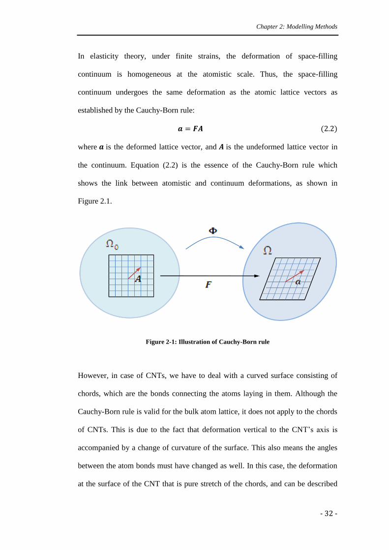
2.2.2 Shift vector
Due to the non-centrosymmetric hexagonal atomic structure of CNTs, the
standard Cauchy-Born rule cannot be applied directly for CNTs because it cannot
satisfy the inner equilibrium of the representative cell. A system is said to be
centrosymmetric when at any time for one point at position there is
always another point at position . For a centrosymmetric lattice there
has to be another lattice pointing the opposite direction from the same atom,
Chapter 2: Modelling Methods
- 34 -
which is not the case for CNTs. The Cauchy-Born rule ensures the equilibrium of
centrosymmetric lattices because the forces of paired lattices are equal and
opposite under homogeneous deformation.
The hexagonal lattice of a graphite sheet, which is called a Bravais multi-lattice, is
not centrosymmetric, however, it consists of two centrosymmetric sub-lattices.
Therefore, it is essential to introduce an in-plane shift vector as a bridge of two
centrosymmetric sub-lattices. The position vectors of multi-lattice, two
centrosymmetric sub-lattices, and an inner displacement of the atom sites are
described in Figure 2.2.
Figure 2-2: Multi-lattice, sub-lattices, and shift vector
Let define the basis vectors of a centrosymmetric sub-lattice, and
be the relative shift vector of two sub-lattices. To reach the required degrees of
freedom, an additional kinematic variable is introduced, by describing the
Chapter 2: Modelling Methods
- 35 -
perturbation of the shift vector, denoted by . The bond vectors (i=1, 2, 3) after
the perturbation are
where are the undeformed bond vectors.
Let , then the bond vectors are
The introducing of shift vector results in differences of solutions in the stress and
modulus fields for materials with centrosymmetric or non-centrosymmetric
atomic structures, which are presented in the following.
2.2.2.1 Centrosymmetric atomic structure
Let define the deformation gradient, from Cauchy-Born rule, we have
Define to be the undeformed bond vector between atom I and J. The bond
length after deformation is
The interatomic potential can be described as
where bond length and bond angle between and , denoted by ,
are
and bond length is
Chapter 2: Modelling Methods
- 36 -
Strain energy density is expressed as
where is the area of the representative atomic cell, and the force tensor can be
expressed as
2.2.2.2 Non-centrosymmetric atomic structure
Let define the inner displacement of a sub-lattice , with the undeformed lattice
vector . Since , the deformed lattice under inner perturbation and
deformation gradient can be written as
Then the bond length between atoms and becomes
Same as before the strain energy density is
The bond angle can be obtained from
Chapter 2: Modelling Methods
- 37 -
As an inner variable, can be computed by minimising the strain energy density
with respect to
which leads to
Then we have
The force tensor is now the direct derivative
The modulus tensor
This is also a footprint of the derivations for dealing with inner displacement
vector in Section 4.1. Wang et al. (2006) pointed out the results obtained without
inner displacement were closer to atomistic simulation and experimental results
than those with inner displacement. But Arroyo and Belytschko (2004) insisted
that, even so, non-relaxation results were theoretically incorrect.
Chapter 2: Modelling Methods
- 38 -
2.3 The Cosserat surface as a shell model
The central idea of Cosserat surface is to consider a thin three-dimensional
classical continuum shell as a two-dimensional Cosserat continuum manifold, i.e.
a Cosserat surface. A displacement field and a rotation field are introduced
specifically, where they are independent of each other. Cosserat continuum theory
is different from classical continuum theory by introducing a displacement field-
independent rotation tensor, which can describe the behaviour of the inner
structure within the surface, i.e. at a micro-level. Cosserat surface theory is to
apply Cosserat continuum theory into a shell model, where the first and second
strain measures are designed to be strain measures of the shell, which leads all
different formulations from original Cosserat continuum theory (Sansour and
Bednarczyk, 1995).
2.3.1 The deformation gradient
Let define a two-dimensional surface, and be the real numbers. The
map
depends on the parameter . (Here is a surface to surface map, as a
counterpart of body to body map Φ, as mentioned in Section 2.2.1.) The reference
configuration is defined by . For simplicity, we write instead
of and instead of , then we have
At time , is a point in the reference configuration and is the point in the
deformed configuration, then the relations hold
Chapter 2: Modelling Methods
- 39 -
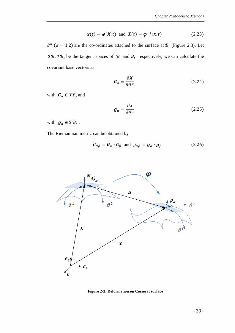
and
are the co-ordinates attached to the surface at , (Figure 2.3). Let
, be the tangent spaces of and respectively, we can calculate the
covariant base vectors as
with , and
with .
The Riemannian metric can be obtained by
and
Figure 2-3: Deformation on Cosserat surface
Chapter 2: Modelling Methods
- 40 -
The determinants of and are indicated by and . The basic skew-
symmetric three-dimensional Levi-Civita tensor, also known as the permutation
tensor, is denoted by
and
where by its Euclidean structure. Here, are set to be 1, 2 or 3. In
absolute notation, it reads
Similarly, the two-dimensional Ricci tensors are
The normal vector is defined by at the reference configuration,
where it is easily seen that . For a curvature tensor , its
components are given by . Also a Cartesian frame is considered
by , and the quantities can be obtained from
which describes the relations of the two base systems.
Chapter 2: Modelling Methods
- 41 -
The deformation gradient is defined as the tangent of the map , ,
where
, or
can be given as the tensor product
The displacement field is introduced by the displacement vector
and we have
and
where comma denotes partial derivatives.
2.3.2 The rotation tensor
One of the assumptions of the shell theory is that a displacement field as well as a
rotation field are attached to the Cosserat surface, both of which are assumed to be
independent of each other. The rotation field is introduced by an orthogonal tensor
which is described by an exponential map
with , and with to be the corresponding axial vector of .
For any , it has a closed expression
If coincides with , the relation gives
Chapter 2: Modelling Methods
- 42 -
So is an eigenvector of . If we use the rotation , where is the
identity tensor, the relation is obtained .
Furthermore, taking the derivative of the relation , one has
Notice that , where is the tangent space of , which
defines the Lie algebra (Hall, 2003), that consists of all the skew-symmetric
tensors. Let be the axial vector of , then one can get the relation
is related to which is the eigenvector of .
Variation of can be given by left or right multiplications
where and are both skew-symmetric.
Let and be the axial vectors of and , the variation of can be derived by
which means , and we have
So
Similarly it can be derived that .
2.3.3 Strain measures
The first Cosserat deformation tensor is

Chapter 2: Modelling Methods
- 43 -
And the second Cosserat deformation tensor is
Alternatively, can be written as
where ( ) denotes a double contraction; the relation holds , where
, are two second order tensors and is the trace operation.
A strain measure can be defined as that vanishes at the reference configuration
where at the reference configuration.
The strain tensors can be decomposed with respect to the tangential base system at
the reference configuration
when writing the displacement and the rotation field in terms of Cartesian
components
,
the strain measures can be finally expressed as
Chapter 2: Modelling Methods
- 44 -
2.3.4 Principle of virtual work
In a pure mechanical theory, the internal potential function for the Cosserat
surface depends on the two strain tensors and
where is the density of the surface. The force tensor and the couple tensor are
defined as
Notice that here is the Boit-like stress tensor, which is different from but related
with the first Piola-Kirchhoff stress tensor in Equation (1.18) and the second
Piola-Kirchhoff stress tensor in Equation (1.8).
For the Cosserat surface, the principle of virtual work holds
While the external virtual work is defined as
Chapter 2: Modelling Methods
- 45 -
where is the density at reference configuration, is the area element of the
curved surface , and is the line element on its boundary , and are the
forces and torques on the surface, and and are corresponding forces on the
boundary.
With these relations and
along with the geometric boundary conditions, equilibrium equations can be
derived:
The first and second variations of the strain measure are
The first and second variations of strain measure can be defined by
So
Chapter 2: Modelling Methods
- 46 -
We write and , and so we have
The vitual principle equation can be expressed as
Since
and with the use of the divergence theorem, it becomes
are the components of the external normal vector at the boundary which
lies on the tangent plane of .
Because and are free variations, we have the localized governing equations
for the equilibrium, the Euler-Lagrange equations in ,
which can be alternatively expressed as
Chapter 2: Modelling Methods
- 47 -
and we also get the natural boundary conditions on
2.4 Potentials
The mechanical properties of CNTs are largely determined by the interatomic
forces, which are governed by the chemical bonds, which are expressed in terms
of interatomic potential models. An ideal potential model should be able to
accurately describe the interactions which bind the atoms together.
Empirical potentials are used extensively, which take simple forms of atomic
positions alone, which provide great advantages in theoretical simulations. Many
interatomic potential models have been developed and reported in the literature,
some of them are simple, while some of them are relatively complicated. Using
different potential models can result in totally different results. Wu et al. (2008)
pointed out that the use of two generations of Brenner potentials results in totally
opposite results in modelling the critical strains of CNTs in tension, as shown in
Figure 2.4, where represents the axisymmetric bifurcation, and
represents the nonaxisymmetric bifurcation. Even by using the same potential
model, the use of different parameters leads to a big difference as well. Wang et
al. (2006) demonstrated the difference in modelling Young’s modulus of CNTs by
using two sets of parameters in Tersoff-Brenner potential, as shown in Figure 2.5.
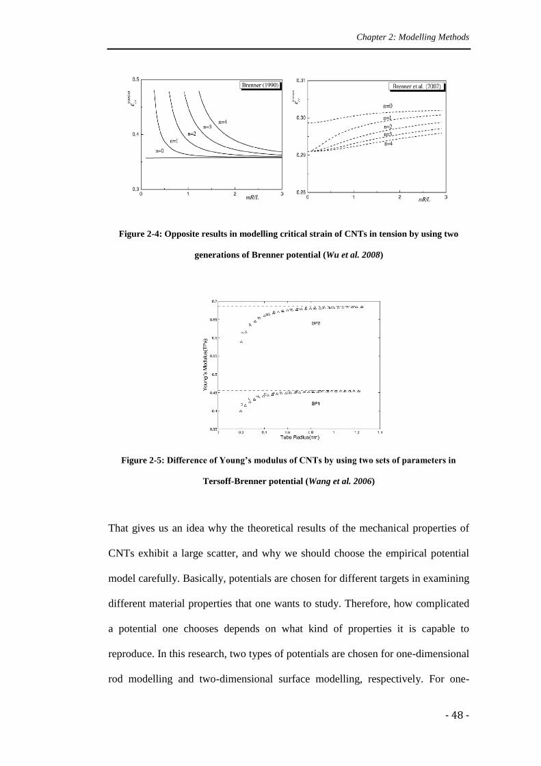
Chapter 2: Modelling Methods
- 48 -
Figure 2-4: Opposite results in modelling critical strain of CNTs in tension by using two
generations of Brenner potential (Wu et al. 2008)
Figure 2-5: Difference of Young’s modulus of CNTs by using two sets of parameters in
Tersoff-Brenner potential (Wang et al. 2006)
That gives us an idea why the theoretical results of the mechanical properties of
CNTs exhibit a large scatter, and why we should choose the empirical potential
model carefully. Basically, potentials are chosen for different targets in examining
different material properties that one wants to study. Therefore, how complicated
a potential one chooses depends on what kind of properties it is capable to
reproduce. In this research, two types of potentials are chosen for one-dimensional
rod modelling and two-dimensional surface modelling, respectively. For one-
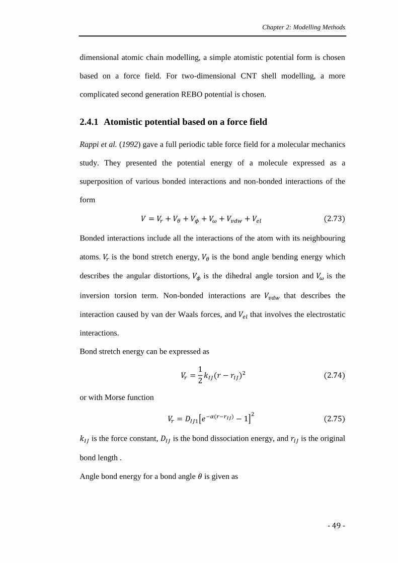
Chapter 2: Modelling Methods
- 49 -
dimensional atomic chain modelling, a simple atomistic potential form is chosen
based on a force field. For two-dimensional CNT shell modelling, a more
complicated second generation REBO potential is chosen.
2.4.1 Atomistic potential based on a force field
Rappi et al. (1992) gave a full periodic table force field for a molecular mechanics
study. They presented the potential energy of a molecule expressed as a
superposition of various bonded interactions and non-bonded interactions of the
form
Bonded interactions include all the interactions of the atom with its neighbouring
atoms. is the bond stretch energy, is the bond angle bending energy which
describes the angular distortions, is the dihedral angle torsion and is the
inversion torsion term. Non-bonded interactions are that describes the
interaction caused by van der Waals forces, and that involves the electrostatic
interactions.
Bond stretch energy can be expressed as
or with Morse function
is the force constant, is the bond dissociation energy, and is the original
bond length .
Angle bond energy for a bond angle is given as
Chapter 2: Modelling Methods
- 50 -
which simplifies to
The torsion potential for a torsion angle is also expressed as a small cosine
Fourier expansion
where is a shape factor.
The inversion term is given as
Van der Waals force interaction is described by a Lennard-Jones 6-12 type
expression
where is the distance between two non- bonded atoms.
Electrostatic interactions are expressed as
where , are the charges and is the distance in angstroms.
Li and Chou (2003) modelled the deformation of CNTs via a structural mechanics
approach, by considering the bonds between two atoms as a load bearing beam
members. They built up the potential as the sum of the total energy due to valence
of bonded interactions and nonbonded interactions
Chapter 2: Modelling Methods
- 51 -
They pointed out that the harmonic approximation is good enough to describe the
energy when the system undergoes small deformations, so they applied the
simplest harmonic forms of the energies and merged the dihedral angle torsion
term and the inversion term into a single term, expressed as
And they were the first ones to point out, through structural mechanics
calculation, that the molecular material parameters , and stand in direct
relation with the structural mechanics parameters of the beam, which is given as
where , , and are three stiffness parameters that describe the stretch,
bending, and torsion properties of the beam member. This has been applied
widely by researchers afterwards into the finite element modelling of CNTs by
setting C-C bond elastic parameters with ANSYS or ABAQUS or other
commercial finite element software.
Meo and Rossi (2006) proposed a finite element model to simulate mechanical
properties of SWCNTs, by using non-linear spring elements to model carbon
bonds.
Chapter 2: Modelling Methods
- 52 -
They pointed out the effects of and can be neglected for uniaxial
loading and small strain assumption, so they only used the first two terms in the
energy form.
The bond energy is chosen as another expression of Morse potential
with parameters for SWCNTs , and
.
The bond angle energy takes the form
with the parameters , and
.
Avila and Lacerda (2008) evaluated Young’s modulus and Poisson ratio of
SWCNTs by the approach of Li and Chou (2003) using the relation between
structural mechanics parameters and molecular material parameters. They
implemented a macro subroutine into ANSYS V.10 and chose
, and .
Dun et al. (2010) applied a stick-spiral model to calculate the constitutive law for
CNTs buckling analysis. They used the potential form
with , and .
Chapter 2: Modelling Methods
- 53 -
Shokrieh and Rafiee (2010) considered the C-C bond as a beam element and
studied Young’s modulus of CNTs by adopting the potential
with and .
Parvaneh and Shariati (2011) studied the effects of defects and loading on the
prediction of Young’s modulus of SWCNTs. They adopted the energy form
with
where and . They took the
dihedral angle torsion and out-of plane torsion into consideration.
Finally, an atomistic potential is chosen in this research by considering the bond
stretch energy and the bond angle energy. And the torsion energy is considered in
one-dimensional deformation embedded in a three-dimensional space. For one-
dimensional deformation embedded in a two-dimensional space, the potential is
taking to be
Chapter 2: Modelling Methods
- 54 -
where , and .
For one-dimensional deformation in a three-dimensional space case, the potential
is expressed as
where , ,
and .
2.4.2 Potential form for SWCNT
In early stages, the potentials used for molecular mechanics were empirical
isotropic pair potentials, e.g. Lennard-Jones potential, Morse potential, etc. They
take the form
while when . is a cut-off radius. In these models, the
potential only depends on the distance between two atoms, and does not consider
the information about the environment of the atom. For example, Morse potential
is given by
Chapter 2: Modelling Methods
- 55 -
Such potentials were used extensively because of their simplicity. However, these
models suffer a major drawback because they do not depend on the atom’s
environment, which gives no difference for a bulk atom and a surface atom.
Therefore, they are inappropriate to apply for Cosserat surface.
In order to involve the bond angle and the neighbouring atoms of a selected atom,
more complicated bond order potential forms were developed, among which
Tersoff and Brenner’s models were proved to be successful.
Brenner (1990) presented a Tersoff-Brenner interatomic potential for carbon as
For atoms and , where is the distance between atoms and , and are
the repulsive and attractive pair terms given by
The parameter and are determined from the known physical
properties of carbon. The function is merely a smooth cutoff function to limit
the range of the potential, and is given by
and is chosen as cutoff radius by Zhang et al. (2002).
The parameter represents a multi-body coupling between the bond from atom I
to atom J and the local environment of atom I, and is given by
Chapter 2: Modelling Methods
- 56 -
where is the distance between atom I and K, is the cutoff function, is
the angle between bonds I-J and I-K, and the function is given by
Two sets of parameters for carbon which is given by Brenner (1990):
1. , , , ,
, , ,
2. , , , ,
, , ,
which gives the equilibrium bond length of CNTs as 0.142 and 0.145nm from the
two sets of parameters respectively (Zhang et al. 2002).
Bao et al. (2004) applied a second-generation reactive empirical bond order
(REBO) potential energy expression for hydrocarbons presented by Brenner
(2002). In the REBO potential, the total potential energy of the system is given by
where is the distance between atoms I and J, and is a many-body empirical
bond order term. and are repulsive and attractive terms.
is a cut-off function which is given by
Chapter 2: Modelling Methods
- 57 -
which is used to cut off the interactions when atoms become too close, where
and .
Brenner et al. (2002) gave the parameters for carbons as
, , , ,
, , , ,
.
where and .
The bond order function is
where
For , , , ,
, , .
For , , , ,
, , .
For , , , ,
, , .
Chapter 2: Modelling Methods
- 58 -
where F is a tricubic spline.
with , and
for C-C bonds. is the dihedral angle among four
atoms, with and .
Since attributes to various radical energies, such as vacancies, it can be
neglected in this research, and describes the conjugate terms of the
interactions between I-J bond, which is also neglected for the computation.
2.5 The finite element approach
2.5.1 The finite element formulation
The governing equations of the Cosserat surface in shell theory have been derived
in Section 2.4. With the energy forms chosen from Section 2.5, the internal
potential can be write as .
Chapter 2: Modelling Methods
- 59 -
We can reformulate
as
To build a finite element formulation, we introduce the Euclidean vectors
and
where are the components of that is the eigenvector of the rotation tensor
.
Define as the external potential with the relation .
Equation (2.119) can now be written as
Chapter 2: Modelling Methods
- 60 -
where , similarly .
Let
then the external work can be expressed as
where vector is the generalized force corresponding to .
2.5.2 Updating method
The updating method is designed to be path independent, following the approach
presented by Sansour and Wagner (2003).
At one loading step, equilibrium equations are in displacement field and
rotation field , with changing of external loading, new state of equilibrium
established in new kinematical fields and . The update of displacement
field naturally goes like
Chapter 2: Modelling Methods
- 61 -
here, is the iteration step, and is load step.
The rotation increment can be obtained by . But
the rotation tensor itself cannot be interpolated, only its rotation parameters can.
Since at the reference configuration, let rotation vector
be given at
nodel points, where at the reference configuration. Instead of
, corresponding and can describe rotation tensor with parameters at
nodal points which can be interpolated in a classical way.
Quaternion is used to relate a product of two vectors and , expressed as
where is a complex number with .
In the quaternion language, the rotation tensor can be written as and
, and we have , which means and are not
independent.
Set
Let and at an iteration step be and , and let and for the iteration
step be and , we have
Then the updated rotation tensor is
Chapter 2: Modelling Methods
- 62 -
Then can be interpolated in the classical way.
2.5.3 Four node element interpolation
The constitutive relations are determined by derivatives of the potentials chosen in
Section 2.5. The finite element equations are based on the formulation of Equation
(2.122). Four node elements are chosen, and same bi-linear interpolations are set
for all components of and . The natural co-ordinates on the surface are
defined as
where define the co-ordinates of a point within the element.
are
the co-ordinates on the edges of the element. are the shape functions
defined as
with - - - - and - - .
For four node element, the displacement field, as well as the rotation field of the
element is in matrix
Chapter 2: Modelling Methods
- 63 -
is at the nodal points of the element. With four nodes and six degrees of
freedom on each node, , and matrix consists of all the shape functions,
.
The solution is achieved using Newton-Raphson iterative method, where the
second derivative of potential with respect to displacement field must
be evaluated, a very involved operation, the details of which are not presented
here.
Chapter 3: Atomic Chain: Cosserat Curve
- 64 -
Chapter 3
Atomic Chain: Cosserat Curve
This chapter is meant as a preparation of a full analysis of carbon nanotube (CNT)
as a cylindrical shell, where we consider a long slender CNT as an atomic chain
model and simulates the deformations of the atomic chain as a one-dimensional
straight line to a curve in two-dimensional space as well as in three-dimensional
one. The equations for Cosserat curve are derived as a step-down of the general
forms of equations in Section 2.3 for Cosserat surface. Atomic chains under
bending, torsion and dynamic loadings are studied in section 3.4. This chapter
aims to produce qualitative results in modelling CNTs’ deformations from
relatively simply one-dimensional Cosserat curve theory, meanwhile it builds a
platform for further development of the quantitative physical meanings from
atomic chain models.
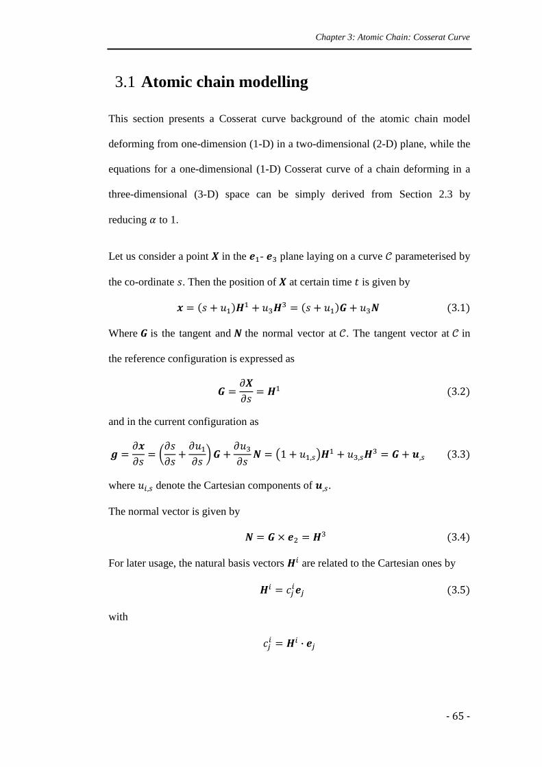
Chapter 3: Atomic Chain: Cosserat Curve
- 65 -
3.1 Atomic chain modelling
This section presents a Cosserat curve background of the atomic chain model
deforming from one-dimension (1-D) in a two-dimensional (2-D) plane, while the
equations for a one-dimensional (1-D) Cosserat curve of a chain deforming in a
three-dimensional (3-D) space can be simply derived from Section 2.3 by
reducing to 1.
Let us consider a point in the - plane laying on a curve parameterised by
the co-ordinate . Then the position of at certain time is given by
Where is the tangent and the normal vector at . The tangent vector at in
the reference configuration is expressed as
and in the current configuration as
where denote the Cartesian components of .
The normal vector is given by
For later usage, the natural basis vectors are related to the Cartesian ones by
(3.5)
with
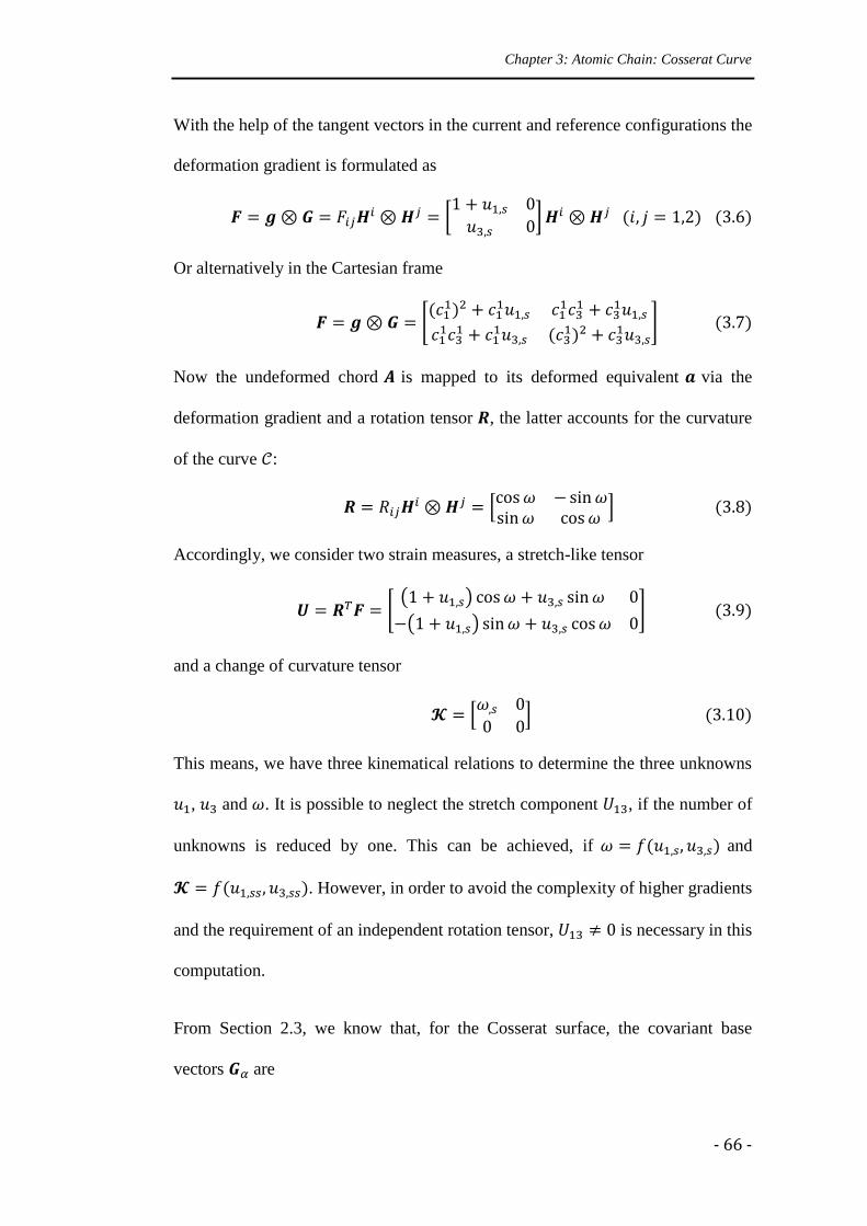
Chapter 3: Atomic Chain: Cosserat Curve
- 66 -
With the help of the tangent vectors in the current and reference configurations the
deformation gradient is formulated as
(3.6)
Or alternatively in the Cartesian frame
(3.7)
Now the undeformed chord is mapped to its deformed equivalent via the
deformation gradient and a rotation tensor , the latter accounts for the curvature
of the curve :
(3.8)
Accordingly, we consider two strain measures, a stretch-like tensor
(3.9)
and a change of curvature tensor
(3.10)
This means, we have three kinematical relations to determine the three unknowns
, and . It is possible to neglect the stretch component , if the number of
unknowns is reduced by one. This can be achieved, if and
. However, in order to avoid the complexity of higher gradients
and the requirement of an independent rotation tensor, is necessary in this
computation.
From Section 2.3, we know that, for the Cosserat surface, the covariant base
vectors are
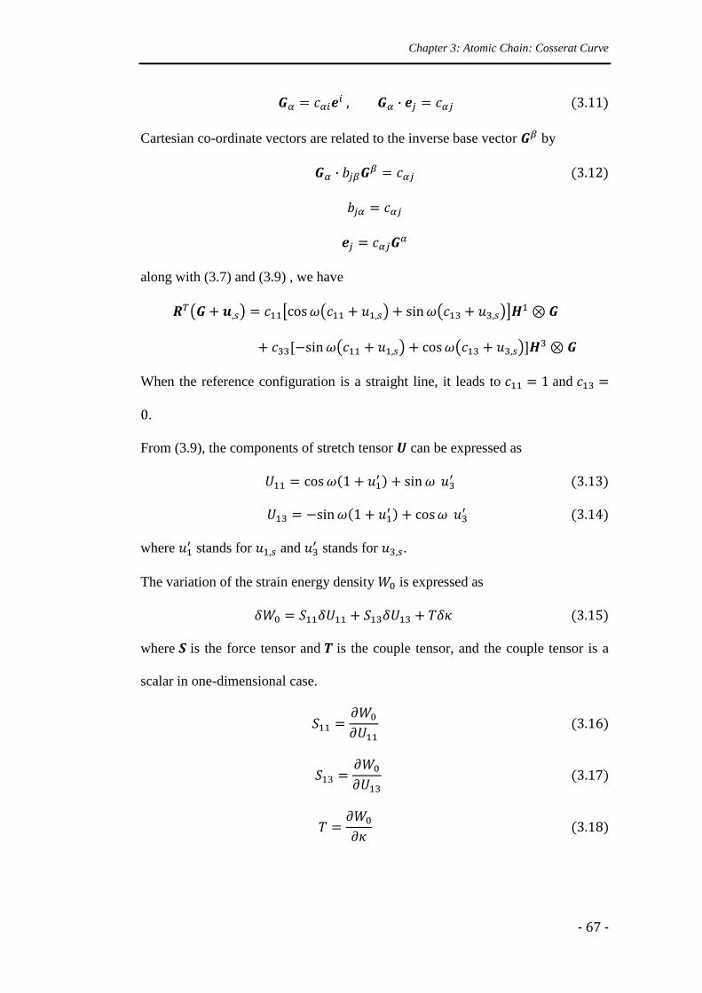
Chapter 3: Atomic Chain: Cosserat Curve
- 67 -
(3.11)
Cartesian co-ordinate vectors are related to the inverse base vector by
(3.12)
along with (3.7) and (3.9) , we have
When the reference configuration is a straight line, it leads to and
.
From (3.9), the components of stretch tensor can be expressed as
(3.13)
(3.14)
where stands for and
stands for .
The variation of the strain energy density is expressed as
(3.15)
where is the force tensor and is the couple tensor, and the couple tensor is a
scalar in one-dimensional case.
Chapter 3: Atomic Chain: Cosserat Curve
- 68 -
The variation of the strain energy density can be further obtained with the
relations between the stretch tensor, the curvature tensor and the deformed
configuration variables , and :
Similarly, the second variations can be derived
The second variation of the strain energy density is
Chapter 3: Atomic Chain: Cosserat Curve
- 69 -
where is the stretch modulus like tensor and is the bending modulus like
tensor, where in one-dimensional case is a scalar, and is the couple modulus
like tensor, which is the second derivative of the strain energy density over the
strain tensor and the curvature tensor. The component of the stretch modulus like
tensor in 11-11 direction gives the tension rigidity which is related to the tension
modulus
The tensor-like bending modulus also known as bending rigidity is related to
bending modulus
The shear modulus is related to tensor-like stretch modulus 11-13 component
The principle of virtual work with total potential holds
(3.23)
where defines the external virtual work, which is given by
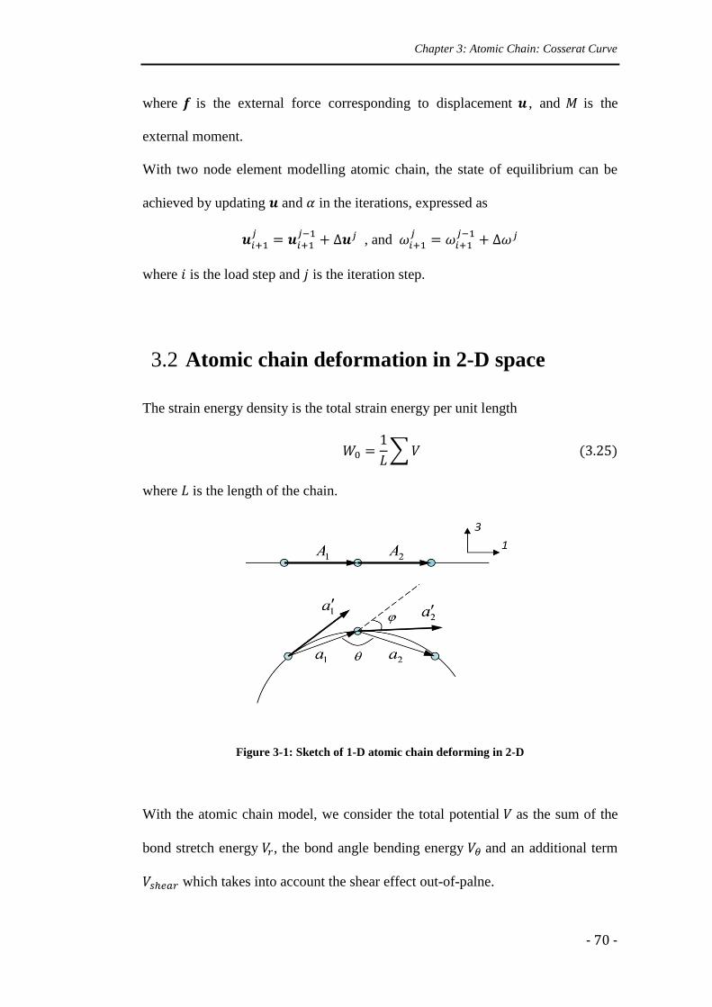
Chapter 3: Atomic Chain: Cosserat Curve
- 70 -
where is the external force corresponding to displacement , and is the
external moment.
With two node element modelling atomic chain, the state of equilibrium can be
achieved by updating and in the iterations, expressed as
, and
where is the load step and is the iteration step.
3.2 Atomic chain deformation in 2-D space
The strain energy density is the total strain energy per unit length
where is the length of the chain.
Figure 3-1: Sketch of 1-D atomic chain deforming in 2-D
With the atomic chain model, we consider the total potential as the sum of the
bond stretch energy , the bond angle bending energy and an additional term
which takes into account the shear effect out-of-palne.
Chapter 3: Atomic Chain: Cosserat Curve
- 71 -
The stretch energy is a function of the bond length , and the bending energy is a
function of the bond angle , as given by the force field mentioned in Section
2.4.1. The additional energy is a function of the shear component of the stretch
tensor .
Figure 3.1 shows a one-dimensional atomic chain deforming in two-dimensional
space. According to the Cauchy-Born rule, the deformed vector on the tangent
plane is
(3.27)
We consider the real deformed vector at the chord of the curve by a
rotation of the tangent vector through an angle . Then the length of is
(3.28)
In equation (3.26), the relation between the deformed bond length and the
reference bond length is
(3.29)
The bond angle in equation (3.26) can be obtained from
(3.30)
Then the total energy in equation (3.26) can be expressed as a function of ,
and .
The standard Cauchy-Born rule provides the change of the bond length via
Equation (3.28), and the independent rotation tensor is related to the bond angle
by Equation (3.30), the choosing of which is explained in Appendix B.

Chapter 3: Atomic Chain: Cosserat Curve
- 72 -
3.3 Atomic chain deformation in 3-D space
As shown in Figure 3.2, in a three-dimensional case, the atomic chain also
deforms in direction 2, so in comparison to the potential in Equation (3.26), we
have three more terms: is the torsion potential as mentioned in section 2.4.1, an
additional shear energy term considering the shear effect from direction 1 to
direction 2, and the spin energy for the rotation in the third dimension
(longitudinal rotation).
Figure 3-2: Sketch of 1-D atomic chain deforming in 3-D
Same as in Equation (3.24) and (3.25), the bond length and the bond angle can
be obtained by
(3.32)
The angle of the torsion is related to the second curvature variable
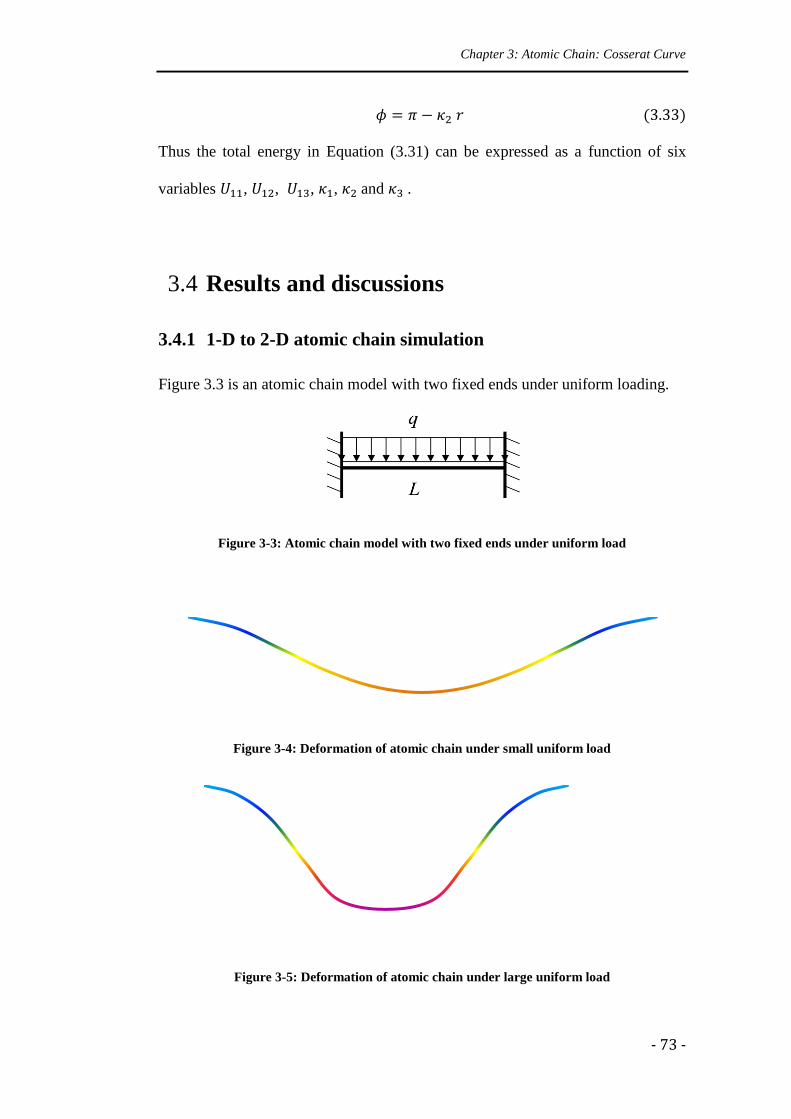
Chapter 3: Atomic Chain: Cosserat Curve
- 73 -
(3.33)
Thus the total energy in Equation (3.31) can be expressed as a function of six
variables , , , , and .
3.4 Results and discussions
3.4.1 1-D to 2-D atomic chain simulation
Figure 3.3 is an atomic chain model with two fixed ends under uniform loading.
Figure 3-3: Atomic chain model with two fixed ends under uniform load
Figure 3-4: Deformation of atomic chain under small uniform load
Figure 3-5: Deformation of atomic chain under large uniform load
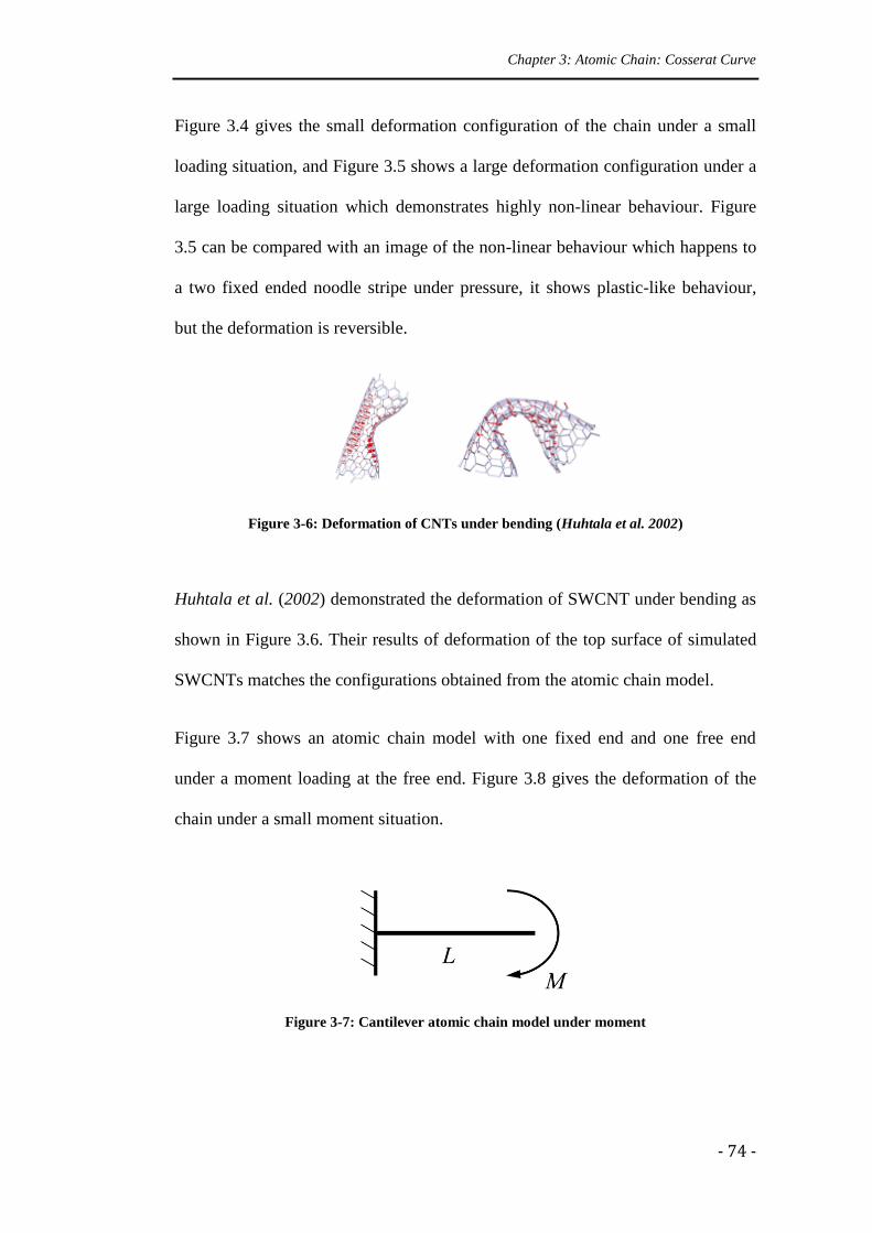
Chapter 3: Atomic Chain: Cosserat Curve
- 74 -
Figure 3.4 gives the small deformation configuration of the chain under a small
loading situation, and Figure 3.5 shows a large deformation configuration under a
large loading situation which demonstrates highly non-linear behaviour. Figure
3.5 can be compared with an image of the non-linear behaviour which happens to
a two fixed ended noodle stripe under pressure, it shows plastic-like behaviour,
but the deformation is reversible.
Figure 3-6: Deformation of CNTs under bending (Huhtala et al. 2002)
Huhtala et al. (2002) demonstrated the deformation of SWCNT under bending as
shown in Figure 3.6. Their results of deformation of the top surface of simulated
SWCNTs matches the configurations obtained from the atomic chain model.
Figure 3.7 shows an atomic chain model with one fixed end and one free end
under a moment loading at the free end. Figure 3.8 gives the deformation of the
chain under a small moment situation.
Figure 3-7: Cantilever atomic chain model under moment
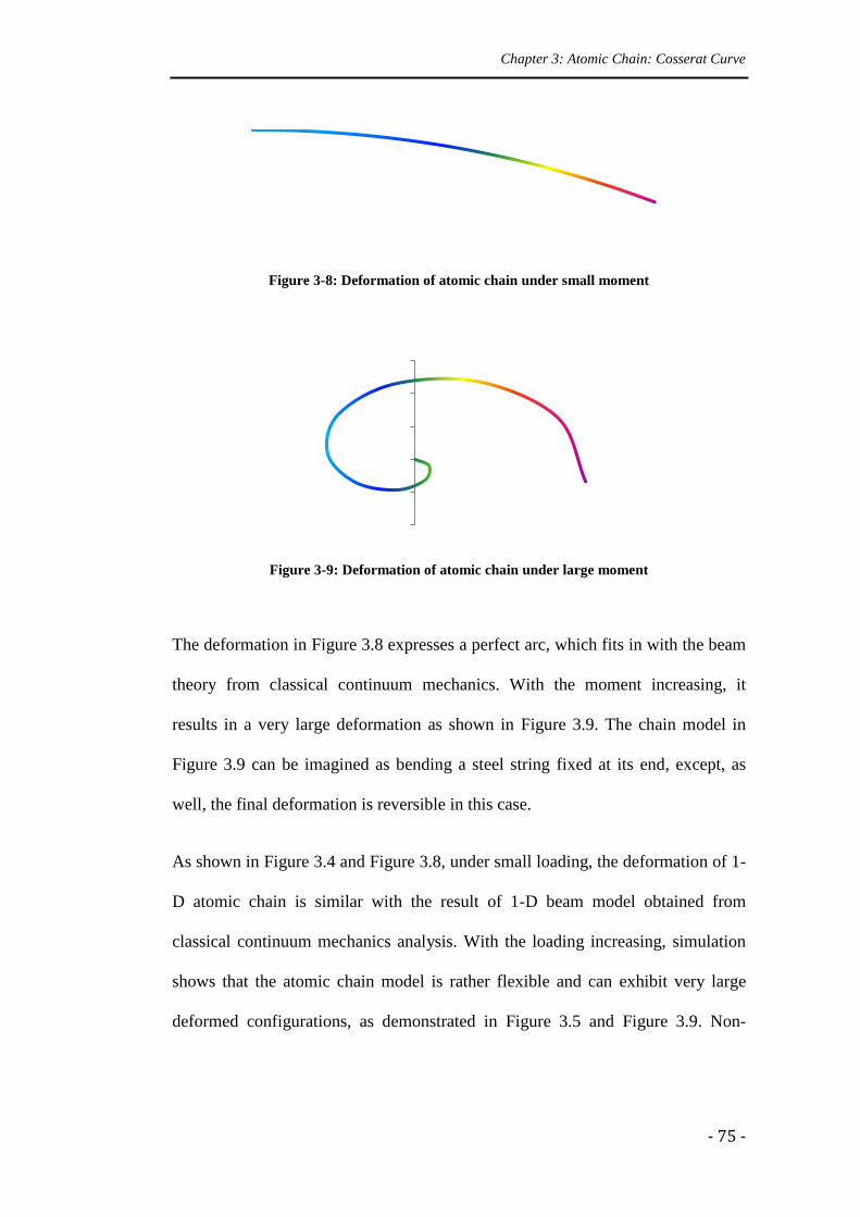
Chapter 3: Atomic Chain: Cosserat Curve
- 75 -
Figure 3-8: Deformation of atomic chain under small moment
Figure 3-9: Deformation of atomic chain under large moment
The deformation in Figure 3.8 expresses a perfect arc, which fits in with the beam
theory from classical continuum mechanics. With the moment increasing, it
results in a very large deformation as shown in Figure 3.9. The chain model in
Figure 3.9 can be imagined as bending a steel string fixed at its end, except, as
well, the final deformation is reversible in this case.
As shown in Figure 3.4 and Figure 3.8, under small loading, the deformation of 1-
D atomic chain is similar with the result of 1-D beam model obtained from
classical continuum mechanics analysis. With the loading increasing, simulation
shows that the atomic chain model is rather flexible and can exhibit very large
deformed configurations, as demonstrated in Figure 3.5 and Figure 3.9. Non-
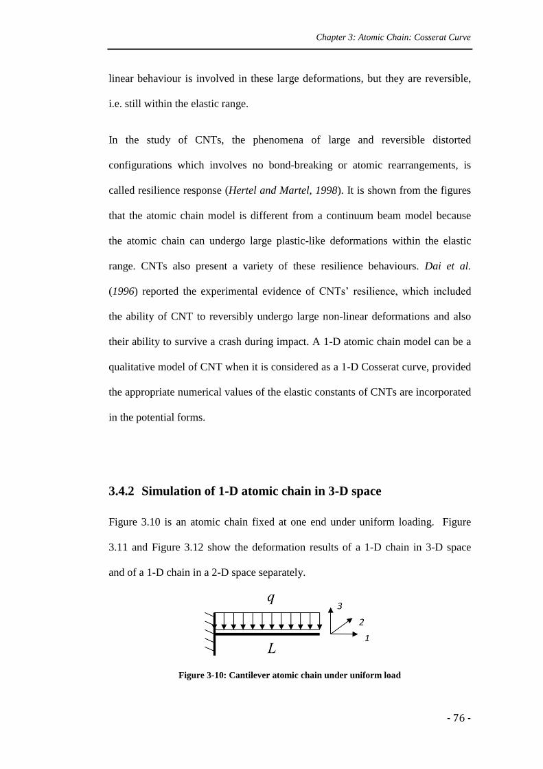
Chapter 3: Atomic Chain: Cosserat Curve
- 76 -
linear behaviour is involved in these large deformations, but they are reversible,
i.e. still within the elastic range.
In the study of CNTs, the phenomena of large and reversible distorted
configurations which involves no bond-breaking or atomic rearrangements, is
called resilience response (Hertel and Martel, 1998). It is shown from the figures
that the atomic chain model is different from a continuum beam model because
the atomic chain can undergo large plastic-like deformations within the elastic
range. CNTs also present a variety of these resilience behaviours. Dai et al.
(1996) reported the experimental evidence of CNTs’ resilience, which included
the ability of CNT to reversibly undergo large non-linear deformations and also
their ability to survive a crash during impact. A 1-D atomic chain model can be a
qualitative model of CNT when it is considered as a 1-D Cosserat curve, provided
the appropriate numerical values of the elastic constants of CNTs are incorporated
in the potential forms.
3.4.2 Simulation of 1-D atomic chain in 3-D space
Figure 3.10 is an atomic chain fixed at one end under uniform loading. Figure
3.11 and Figure 3.12 show the deformation results of a 1-D chain in 3-D space
and of a 1-D chain in a 2-D space separately.
Figure 3-10: Cantilever atomic chain under uniform load
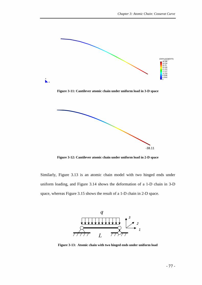
Chapter 3: Atomic Chain: Cosserat Curve
- 77 -
Figure 3-11: Cantilever atomic chain under uniform load in 3-D space
Figure 3-12: Cantilever atomic chain under uniform load in 2-D space
Similarly, Figure 3.13 is an atomic chain model with two hinged ends under
uniform loading, and Figure 3.14 shows the deformation of a 1-D chain in 3-D
space, whereas Figure 3.15 shows the result of a 1-D chain in 2-D space.
Figure 3-13: Atomic chain with two hinged ends under uniform load
-38.11
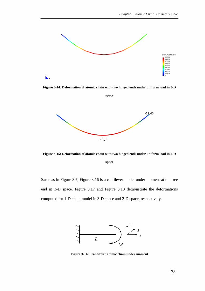
Chapter 3: Atomic Chain: Cosserat Curve
- 78 -
Figure 3-14: Deformation of atomic chain with two hinged ends under uniform load in 3-D
space
Figure 3-15: Deformation of atomic chain with two hinged ends under uniform load in 2-D
space
Same as in Figure 3.7, Figure 3.16 is a cantilever model under moment at the free
end in 3-D space. Figure 3.17 and Figure 3.18 demonstrate the deformations
computed for 1-D chain model in 3-D space and 2-D space, respectively.
Figure 3-16: Cantilever atomic chain under moment
-21.78
-12.45
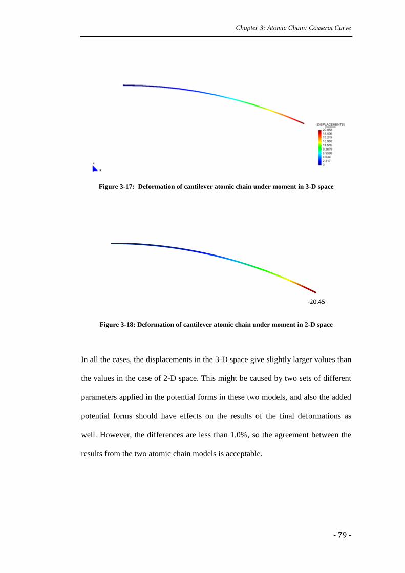
Chapter 3: Atomic Chain: Cosserat Curve
- 79 -
Figure 3-17: Deformation of cantilever atomic chain under moment in 3-D space
Figure 3-18: Deformation of cantilever atomic chain under moment in 2-D space
In all the cases, the displacements in the 3-D space give slightly larger values than
the values in the case of 2-D space. This might be caused by two sets of different
parameters applied in the potential forms in these two models, and also the added
potential forms should have effects on the results of the final deformations as
well. However, the differences are less than 1.0%, so the agreement between the
results from the two atomic chain models is acceptable.
-20.45
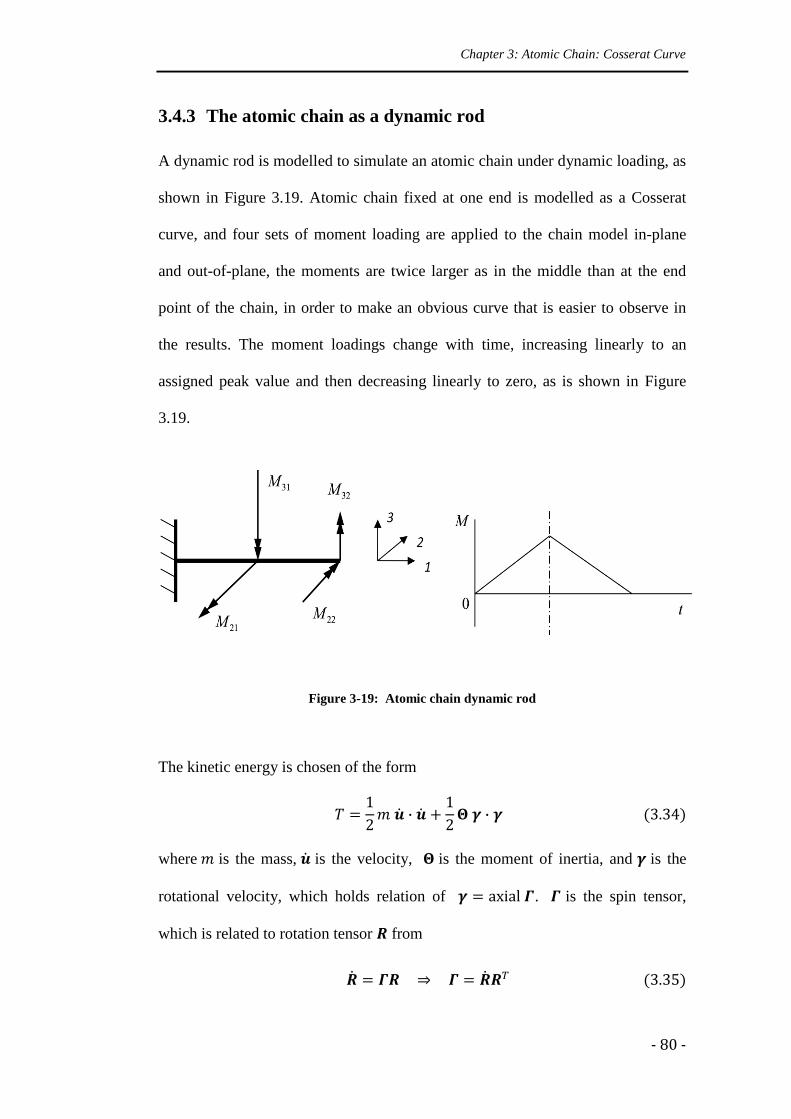
Chapter 3: Atomic Chain: Cosserat Curve
- 80 -
3.4.3 The atomic chain as a dynamic rod
A dynamic rod is modelled to simulate an atomic chain under dynamic loading, as
shown in Figure 3.19. Atomic chain fixed at one end is modelled as a Cosserat
curve, and four sets of moment loading are applied to the chain model in-plane
and out-of-plane, the moments are twice larger as in the middle than at the end
point of the chain, in order to make an obvious curve that is easier to observe in
the results. The moment loadings change with time, increasing linearly to an
assigned peak value and then decreasing linearly to zero, as is shown in Figure
3.19.
Figure 3-19: Atomic chain dynamic rod
The kinetic energy is chosen of the form
where is the mass, is the velocity, is the moment of inertia, and is the
rotational velocity, which holds relation of . is the spin tensor,
which is related to rotation tensor from
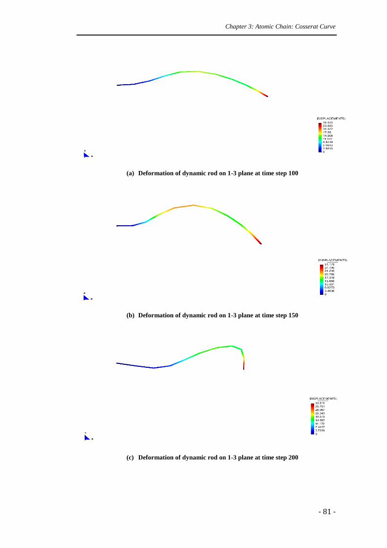
Chapter 3: Atomic Chain: Cosserat Curve
- 81 -
(a) Deformation of dynamic rod on 1-3 plane at time step 100
(b) Deformation of dynamic rod on 1-3 plane at time step 150
(c) Deformation of dynamic rod on 1-3 plane at time step 200
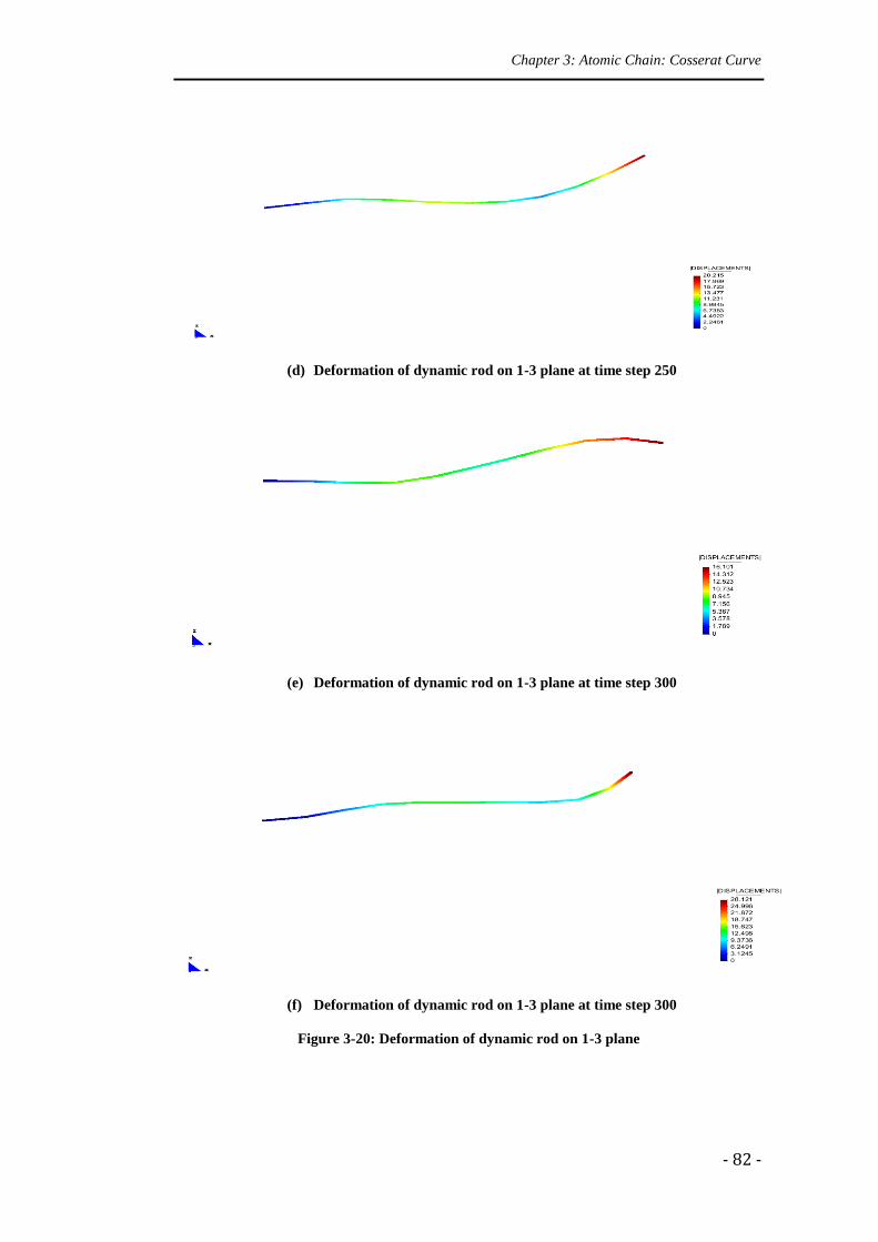
Chapter 3: Atomic Chain: Cosserat Curve
- 82 -
(d) Deformation of dynamic rod on 1-3 plane at time step 250
(e) Deformation of dynamic rod on 1-3 plane at time step 300
(f) Deformation of dynamic rod on 1-3 plane at time step 300
Figure 3-20: Deformation of dynamic rod on 1-3 plane
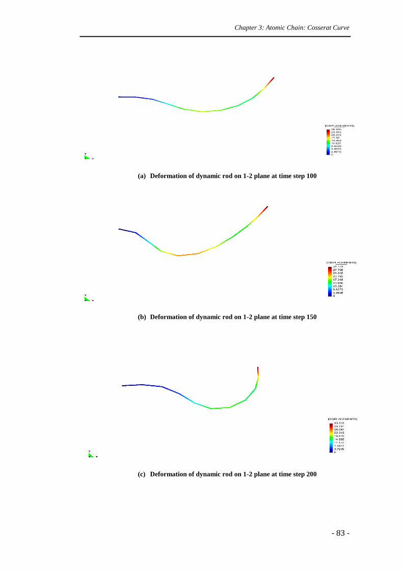
Chapter 3: Atomic Chain: Cosserat Curve
- 83 -
(a) Deformation of dynamic rod on 1-2 plane at time step 100
(b) Deformation of dynamic rod on 1-2 plane at time step 150
(c) Deformation of dynamic rod on 1-2 plane at time step 200
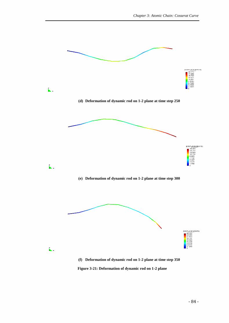
Chapter 3: Atomic Chain: Cosserat Curve
- 84 -
(d) Deformation of dynamic rod on 1-2 plane at time step 250
(e) Deformation of dynamic rod on 1-2 plane at time step 300
(f) Deformation of dynamic rod on 1-2 plane at time step 350
Figure 3-21: Deformation of dynamic rod on 1-2 plane
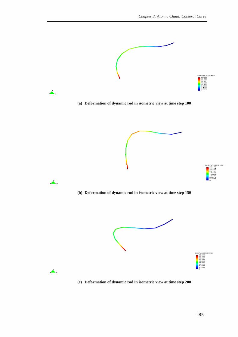
Chapter 3: Atomic Chain: Cosserat Curve
- 85 -
(a) Deformation of dynamic rod in isometric view at time step 100
(b) Deformation of dynamic rod in isometric view at time step 150
(c) Deformation of dynamic rod in isometric view at time step 200
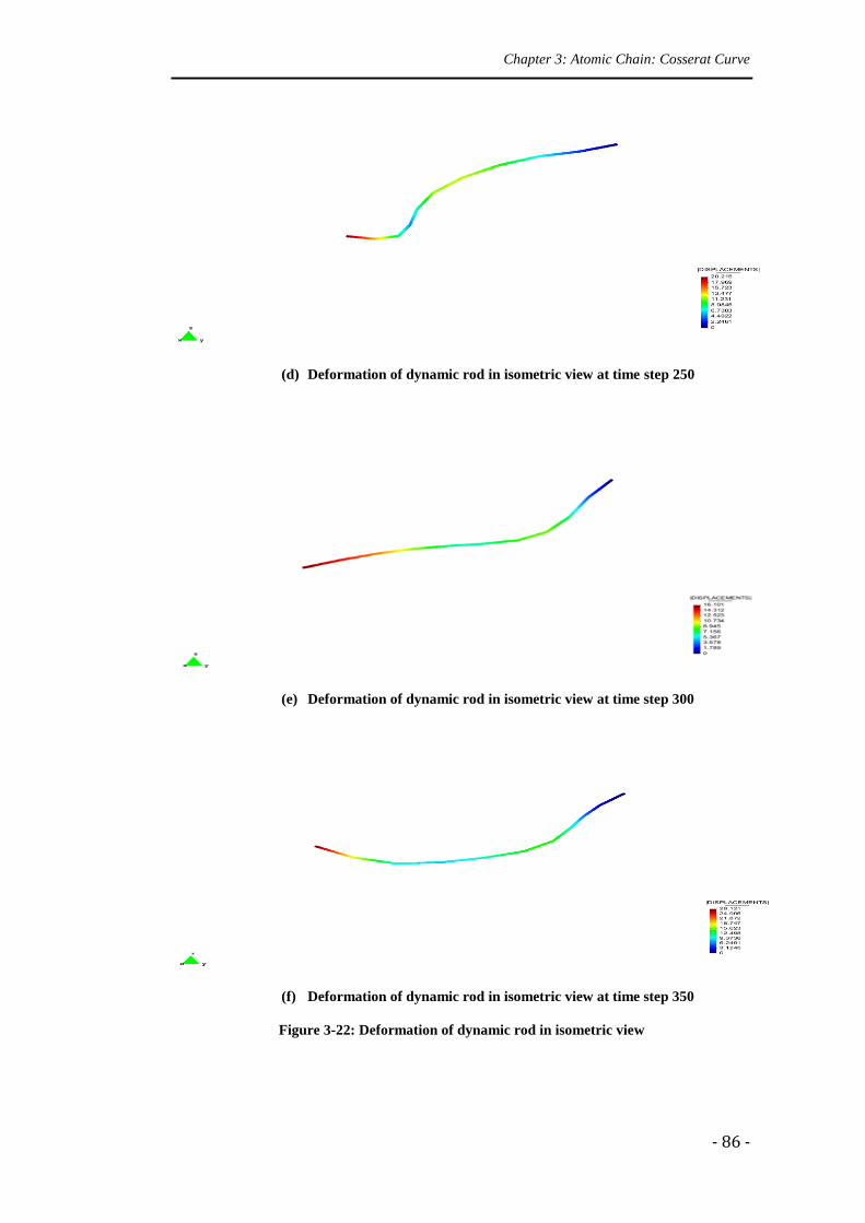
Chapter 3: Atomic Chain: Cosserat Curve
- 86 -
(d) Deformation of dynamic rod in isometric view at time step 250
(e) Deformation of dynamic rod in isometric view at time step 300
(f) Deformation of dynamic rod in isometric view at time step 350
Figure 3-22: Deformation of dynamic rod in isometric view
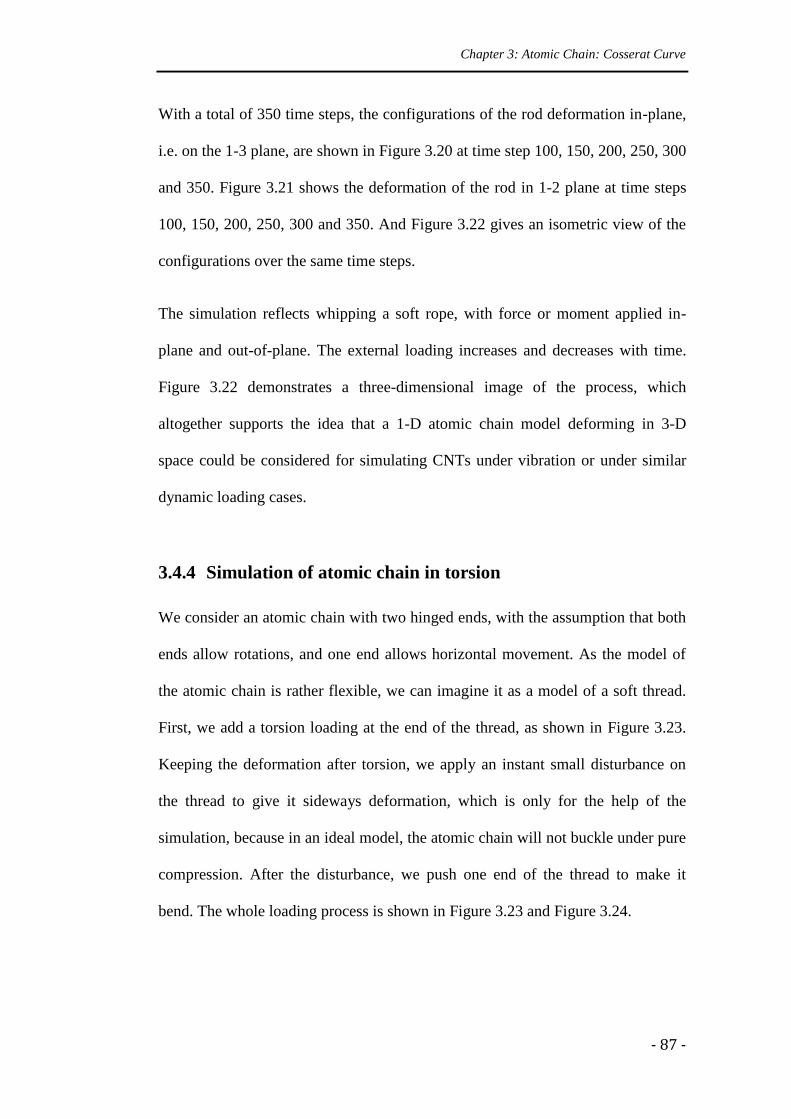
Chapter 3: Atomic Chain: Cosserat Curve
- 87 -
With a total of 350 time steps, the configurations of the rod deformation in-plane,
i.e. on the 1-3 plane, are shown in Figure 3.20 at time step 100, 150, 200, 250, 300
and 350. Figure 3.21 shows the deformation of the rod in 1-2 plane at time steps
100, 150, 200, 250, 300 and 350. And Figure 3.22 gives an isometric view of the
configurations over the same time steps.
The simulation reflects whipping a soft rope, with force or moment applied in-
plane and out-of-plane. The external loading increases and decreases with time.
Figure 3.22 demonstrates a three-dimensional image of the process, which
altogether supports the idea that a 1-D atomic chain model deforming in 3-D
space could be considered for simulating CNTs under vibration or under similar
dynamic loading cases.
3.4.4 Simulation of atomic chain in torsion
We consider an atomic chain with two hinged ends, with the assumption that both
ends allow rotations, and one end allows horizontal movement. As the model of
the atomic chain is rather flexible, we can imagine it as a model of a soft thread.
First, we add a torsion loading at the end of the thread, as shown in Figure 3.23.
Keeping the deformation after torsion, we apply an instant small disturbance on
the thread to give it sideways deformation, which is only for the help of the
simulation, because in an ideal model, the atomic chain will not buckle under pure
compression. After the disturbance, we push one end of the thread to make it
bend. The whole loading process is shown in Figure 3.23 and Figure 3.24.
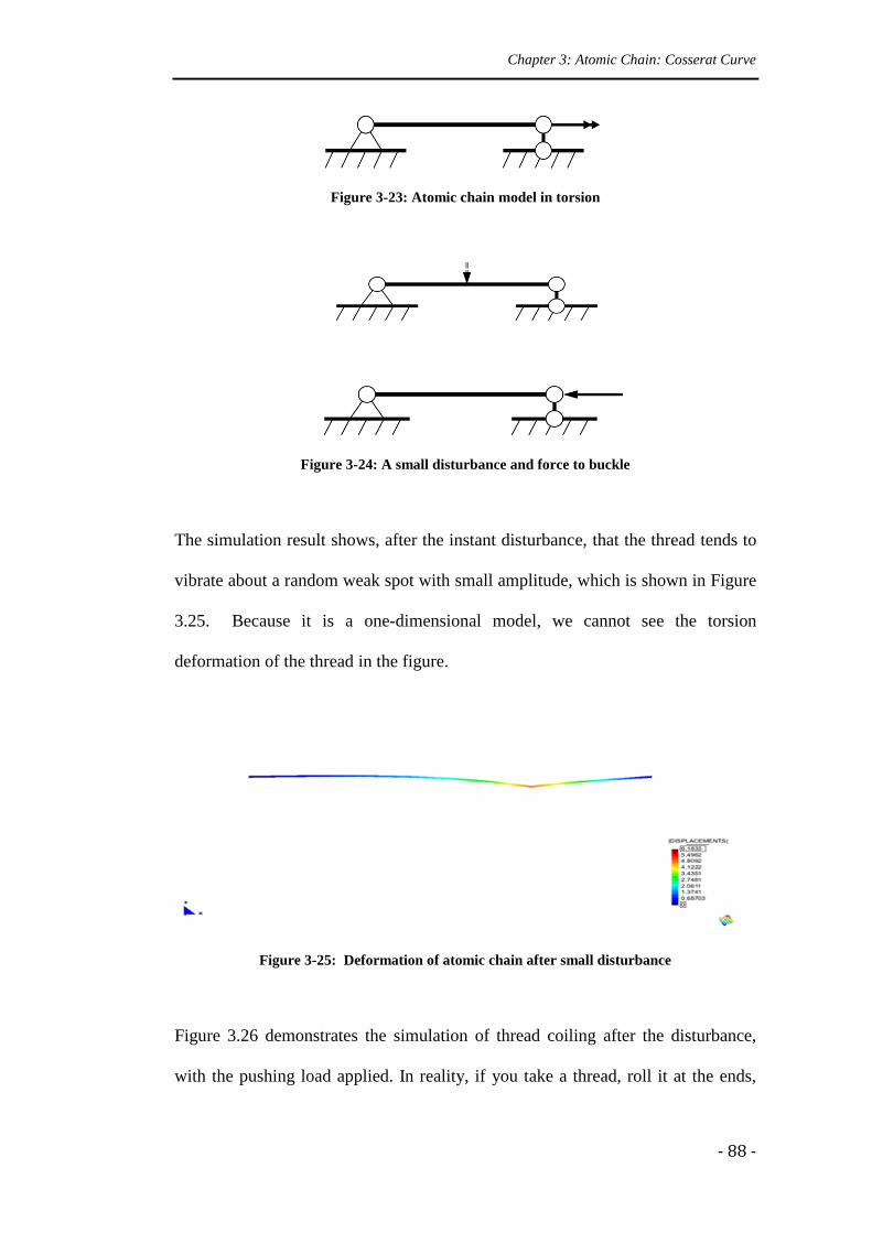
Chapter 3: Atomic Chain: Cosserat Curve
- 88 -
Figure 3-23: Atomic chain model in torsion
Figure 3-24: A small disturbance and force to buckle
The simulation result shows, after the instant disturbance, that the thread tends to
vibrate about a random weak spot with small amplitude, which is shown in Figure
3.25. Because it is a one-dimensional model, we cannot see the torsion
deformation of the thread in the figure.
Figure 3-25: Deformation of atomic chain after small disturbance
Figure 3.26 demonstrates the simulation of thread coiling after the disturbance,
with the pushing load applied. In reality, if you take a thread, roll it at the ends,
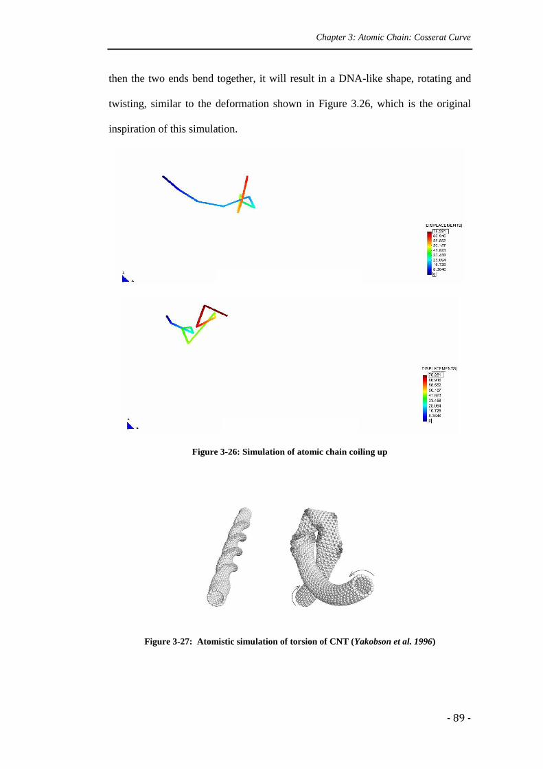
Chapter 3: Atomic Chain: Cosserat Curve
- 89 -
then the two ends bend together, it will result in a DNA-like shape, rotating and
twisting, similar to the deformation shown in Figure 3.26, which is the original
inspiration of this simulation.
Figure 3-26: Simulation of atomic chain coiling up
Figure 3-27: Atomistic simulation of torsion of CNT (Yakobson et al. 1996)
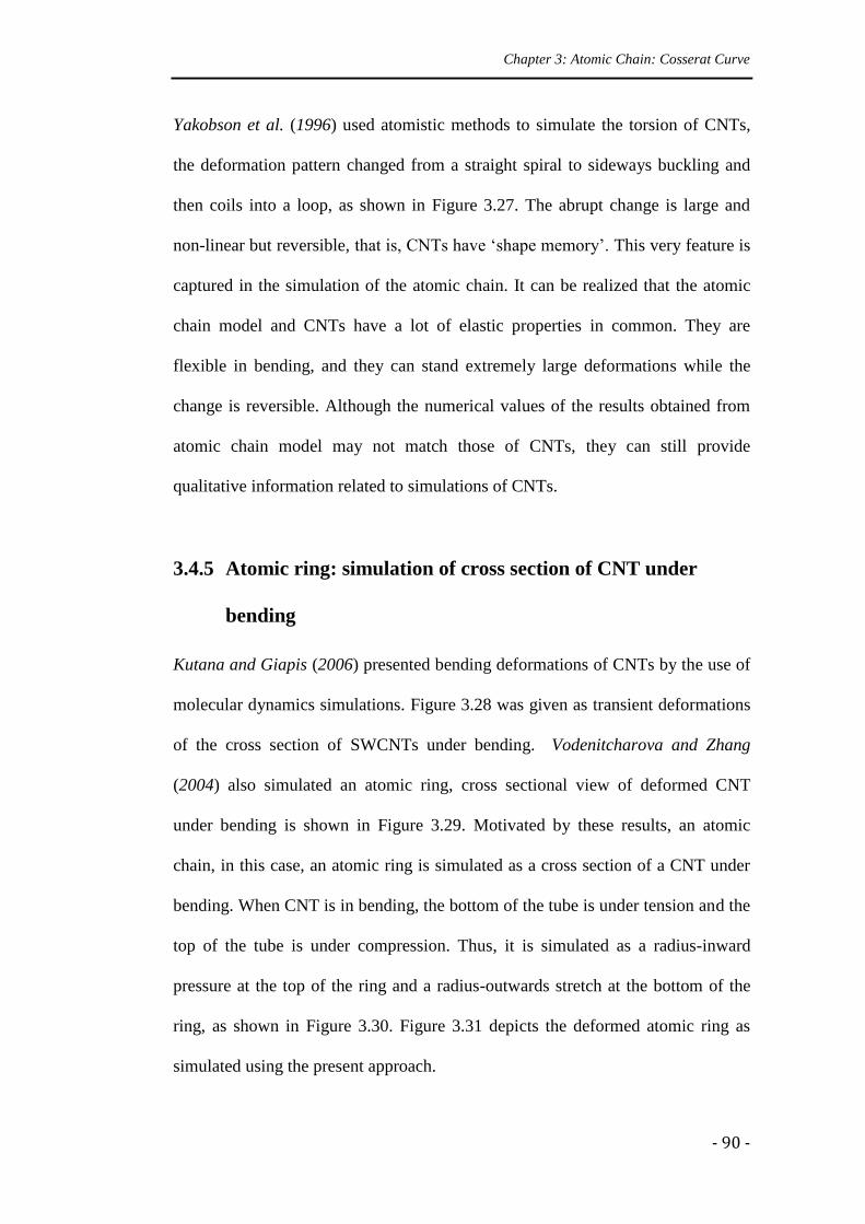
Chapter 3: Atomic Chain: Cosserat Curve
- 90 -
Yakobson et al. (1996) used atomistic methods to simulate the torsion of CNTs,
the deformation pattern changed from a straight spiral to sideways buckling and
then coils into a loop, as shown in Figure 3.27. The abrupt change is large and
non-linear but reversible, that is, CNTs have ‘shape memory’. This very feature is
captured in the simulation of the atomic chain. It can be realized that the atomic
chain model and CNTs have a lot of elastic properties in common. They are
flexible in bending, and they can stand extremely large deformations while the
change is reversible. Although the numerical values of the results obtained from
atomic chain model may not match those of CNTs, they can still provide
qualitative information related to simulations of CNTs.
3.4.5 Atomic ring: simulation of cross section of CNT under
bending
Kutana and Giapis (2006) presented bending deformations of CNTs by the use of
molecular dynamics simulations. Figure 3.28 was given as transient deformations
of the cross section of SWCNTs under bending. Vodenitcharova and Zhang
(2004) also simulated an atomic ring, cross sectional view of deformed CNT
under bending is shown in Figure 3.29. Motivated by these results, an atomic
chain, in this case, an atomic ring is simulated as a cross section of a CNT under
bending. When CNT is in bending, the bottom of the tube is under tension and the
top of the tube is under compression. Thus, it is simulated as a radius-inward
pressure at the top of the ring and a radius-outwards stretch at the bottom of the
ring, as shown in Figure 3.30. Figure 3.31 depicts the deformed atomic ring as
simulated using the present approach.
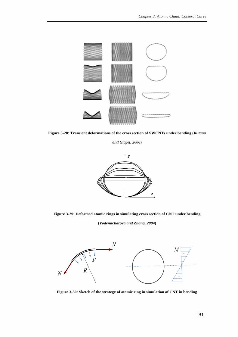
Chapter 3: Atomic Chain: Cosserat Curve
- 91 -
Figure 3-28: Transient deformations of the cross section of SWCNTs under bending (Kutana
and Giapis, 2006)
Figure 3-29: Deformed atomic rings in simulating cross section of CNT under bending
(Vodenitcharova and Zhang, 2004)
Figure 3-30: Sketch of the strategy of atomic ring in simulation of CNT in bending
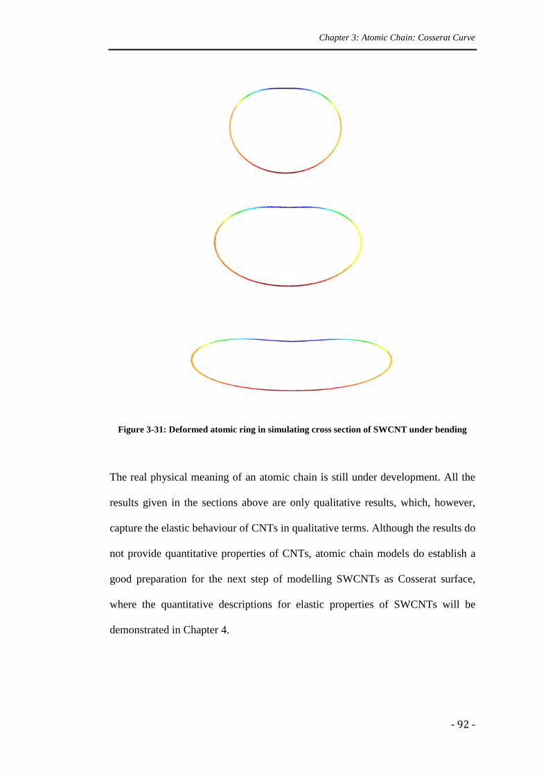
Chapter 3: Atomic Chain: Cosserat Curve
- 92 -
Figure 3-31: Deformed atomic ring in simulating cross section of SWCNT under bending
The real physical meaning of an atomic chain is still under development. All the
results given in the sections above are only qualitative results, which, however,
capture the elastic behaviour of CNTs in qualitative terms. Although the results do
not provide quantitative properties of CNTs, atomic chain models do establish a
good preparation for the next step of modelling SWCNTs as Cosserat surface,
where the quantitative descriptions for elastic properties of SWCNTs will be
demonstrated in Chapter 4.
Chapter 4: Single-walled Carbon Nanotube: Cosserat Surface
- 93 -
Chapter 4
Single-walled Carbon Nanotube:
Cosserat Surface
This chapter applies the Cosserat surface theory in modelling and simulating
carbon nanotubes’ (CNTs) behaviours. CNTs are modelled as unrolled two-
dimensional graphite sheets or as cylindrical shell models. Potential forms are
applied as described in Section 2.4, where, in this chapter, the in-plane and out-of-
plane contributions are considered for the calculation of stress fields and moment
fields. The mechanical properties of CNTs, such as Young’s modulus and Poisson
ratio are predicted as tension and bending models, and the deformations of CNTs
under bending, compression and torsion loadings are simulated in Section 4.2 to
Section 4.6.
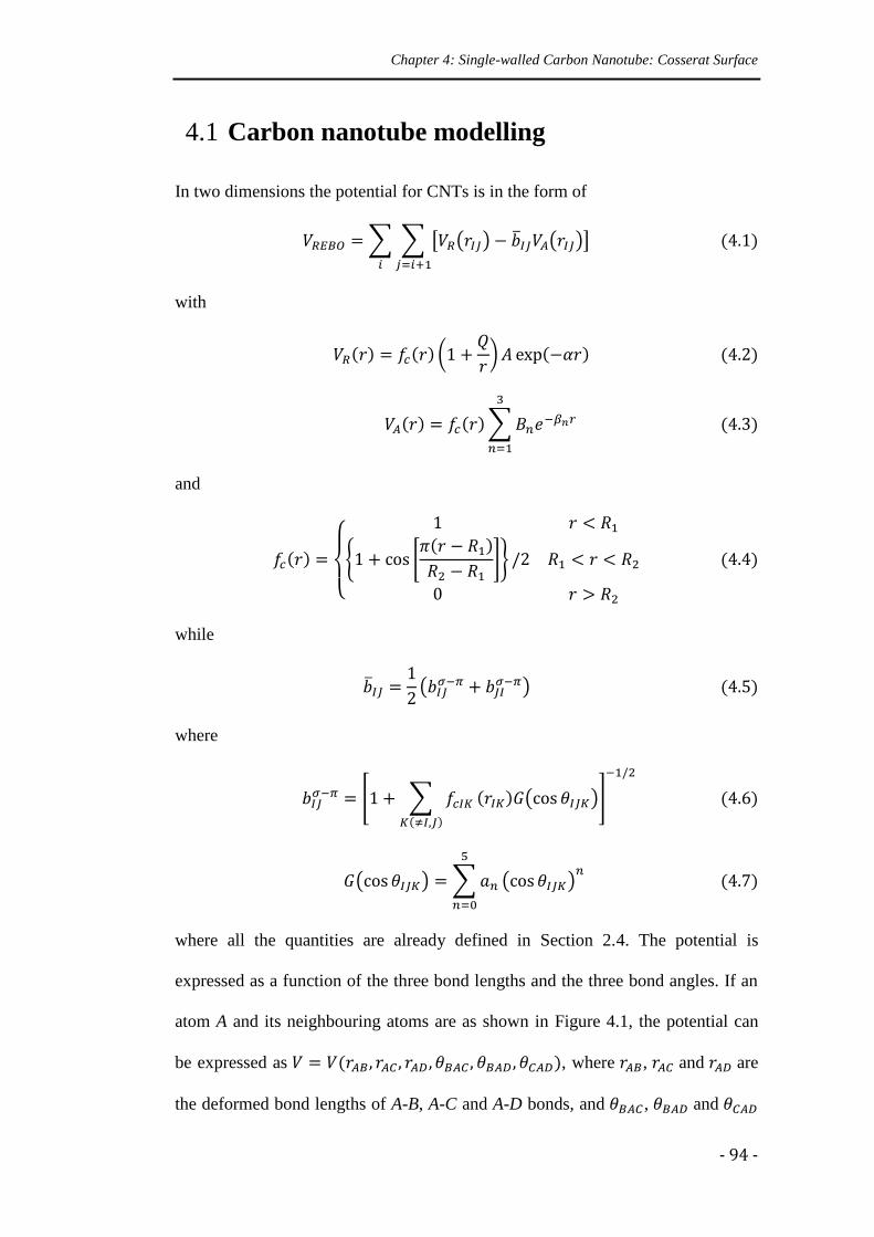
Chapter 4: Single-walled Carbon Nanotube: Cosserat Surface
- 94 -
4.1 Carbon nanotube modelling
In two dimensions the potential for CNTs is in the form of
with
and
while
where
where all the quantities are already defined in Section 2.4. The potential is
expressed as a function of the three bond lengths and the three bond angles. If an
atom A and its neighbouring atoms are as shown in Figure 4.1, the potential can
be expressed as , where , and are
the deformed bond lengths of A-B, A-C and A-D bonds, and , and
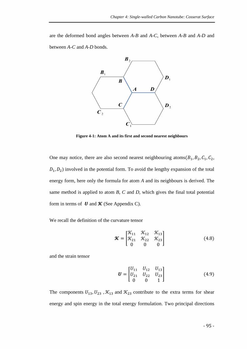
Chapter 4: Single-walled Carbon Nanotube: Cosserat Surface
- 95 -
are the deformed bond angles between A-B and A-C, between A-B and A-D and
between A-C and A-D bonds.
Figure 4-1: Atom A and its first and second nearest neighbours
One may notice, there are also second nearest neighbouring atoms ,
) involved in the potential form. To avoid the lengthy expansion of the total
energy form, here only the formula for atom A and its neighbours is derived. The
same method is applied to atom B, C and D, which gives the final total potential
form in terms of and (See Appendix C).
We recall the definition of the curvature tensor
and the strain tensor
The components and contribute to the extra terms for shear
energy and spin energy in the total energy formulation. Two principal directions
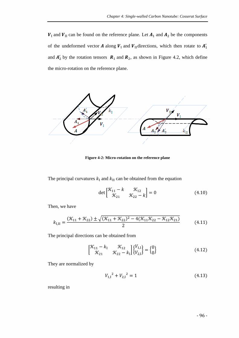
Chapter 4: Single-walled Carbon Nanotube: Cosserat Surface
- 96 -
and can be found on the reference plane. Let and be the components
of the undeformed vector along and directions, which then rotate to
and by the rotation tensors and , as shown in Figure 4.2, which define
the micro-rotation on the reference plane.
Figure 4-2: Micro-rotation on the reference plane
The principal curvatures and can be obtained from the equation
Then, we have
The principal directions can be obtained from
They are normalized by
resulting in
Chapter 4: Single-walled Carbon Nanotube: Cosserat Surface
- 97 -
Thus, the principal directions and and are obtained as
The lattice vector is the vector that the undeformed lattice vector rotates to
after applying the micro-rotation tensor, which is given by
where
Finally
Chapter 4: Single-walled Carbon Nanotube: Cosserat Surface
- 98 -
The final deformed lattice vector is obtained after rotating by then after
stretching by , which is expressed as
The vector length after stretch is
The strain energy density is the total potential of the atom over the area
where , is the undeformed bond length, and
Considering the shift vector
Since the length doesn’t change during the rotation, the deformed bond length
only depends on the strain tensor
Chapter 4: Single-walled Carbon Nanotube: Cosserat Surface
- 99 -
where ,
and are the undeformed bond vectors between A-B, A-C and
A-D atoms.
On the other hand, the bond angles are related to the curvature tensor
The bond angle between A-B and A-C bond can be obtained from
Similarly, we can get the other two bond angles from
Define the bond lengths , , as (i=1,2,3) and the bond angles ,
, as (i=1,2,3), then the potential can be expressed in terms of
and . For simplicity, we write instead of to present the strain energy
density for the rest of this section. Then the internal degree of freedom can be
determined by minimizing the strain energy density with respect to
Strain energy density W again can be written as a function of the strain tensor
and the curvature tensor
Chapter 4: Single-walled Carbon Nanotube: Cosserat Surface
- 100 -
The force tensor can be obtained from
where
The couple tensor can be calculated from
where
The tensor-like stretch modulus reads
with the relation of
one can derive
Then is obtained as
Chapter 4: Single-walled Carbon Nanotube: Cosserat Surface
- 101 -
where
The tensor-like bending modulus reads
Similarly from
Chapter 4: Single-walled Carbon Nanotube: Cosserat Surface
- 102 -
where
Chapter 4: Single-walled Carbon Nanotube: Cosserat Surface
- 103 -
In the non-linear calculation, the minimizing of the strain energy density
with respect to carries out by an updating procedure where the
change of is calculated by
By inserting into the potential, the stress fields and the modulus fields can be
calculated via a finite element method presented in Section 2.5.
4.2 Graphite sheet: Young’s modulus and Poisson
ratio
Ijimia (1991) discovered CNTs and predicted SWCNTs’ Young’s modulus to be
about 1TPa. The following years much experimental research had been carried out
to confirm CNTs’ Young’s modulus. Tension tests, bending methods, thermal
vibration tests had been applied, and the experimental results of Young’s modulus
for SWCNTs ranged from 0.81TPa to 1.28TPa (Wong et al. 1997, Krishnan et al.
1998, Salvatat et al. 1999). Meanwhile, some researchers concentrated on
theoretical studies of the elastic modulus of CNTs. Various theories and
Chapter 4: Single-walled Carbon Nanotube: Cosserat Surface
- 104 -
methodologies had been presented, and the reported numerical values for Young’s
modulus of SWCNTs ranged from 0.5TPa to 6TPa, as shown in Table 4.1. The
experimental data demonstrated a large scatter already due to the high frequencies
of errors from machines and manual processing at the nano-scale. Compared with
a range of 0.47TPa from experimental results, more surprisingly the theoretical
results have a range of scatter up to 5.5TPa. Yakobson (1996) first addressed this
ridiculous large scatter of the reported results for CNTs’ Young’s modulus, which
is now known as ‘Yakobson’s paradox’. Huang et al. (2006) discussed this issue
and identified the cause of ‘Yakobson’s paradox’ as being the ‘ill-defined’ CNTs’
wall thickness from various theories and methodologies and also different types of
loading situations.
Theoretically, the tension rigidity, or just ‘ ’, should be good enough to present
the elastic tension properties of CNTs, however, to compare with other authors’
results, here we apply the linear classical continuum mechanics assumption of
shell theory, which leads us to solve for Young’s modulus , Poisson’s ratio ,
and a case by case defined wall thickness . The tension rigidity is the 11-11
component of the stretch modulus
Poisson’s ratio is captured in the 11-22 component of the stretch modulus-like
tensor
and the bending rigidity is the dominating component in the bending modulus
defined as
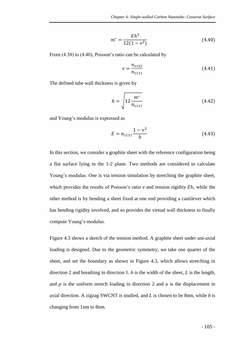
Chapter 4: Single-walled Carbon Nanotube: Cosserat Surface
- 105 -
From (4.38) to (4.40), Poisson’s ratio can be calculated by
The defined tube wall thickness is given by
and Young’s modulus is expressed as
In this section, we consider a graphite sheet with the reference configuration being
a flat surface lying in the 1-2 plane. Two methods are considered to calculate
Young’s modulus. One is via tension simulation by stretching the graphite sheet,
which provides the results of Poisson’s ratio and tension rigidity , while the
other method is by bending a sheet fixed at one end providing a cantilever which
has bending rigidity involved, and so provides the virtual wall thickness to finally
compute Young’s modulus.
Figure 4.3 shows a sketch of the tension method. A graphite sheet under uni-axial
loading is designed. Due to the geometric symmetry, we take one quarter of the
sheet, and set the boundary as shown in Figure 4.3, which allows stretching in
direction 2 and breathing in direction 1. b is the width of the sheet, L is the length,
and p is the uniform stretch loading in direction 2 and u is the displacement in
axial direction. A zigzag SWCNT is studied, and L is chosen to be 8nm, while b is
changing from 1nm to 8nm.
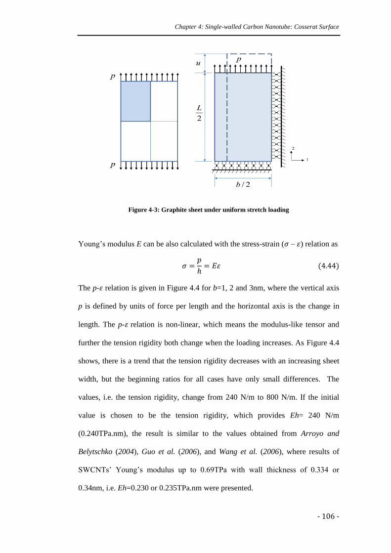
Chapter 4: Single-walled Carbon Nanotube: Cosserat Surface
- 106 -
Figure 4-3: Graphite sheet under uniform stretch loading
Young’s modulus E can be also calculated with the stress-strain ( – ) relation as
The p- relation is given in Figure 4.4 for b=1, 2 and 3nm, where the vertical axis
p is defined by units of force per length and the horizontal axis is the change in
length. The p- relation is non-linear, which means the modulus-like tensor and
further the tension rigidity both change when the loading increases. As Figure 4.4
shows, there is a trend that the tension rigidity decreases with an increasing sheet
width, but the beginning ratios for all cases have only small differences. The
values, i.e. the tension rigidity, change from 240 N/m to 800 N/m. If the initial
value is chosen to be the tension rigidity, which provides Eh= 240 N/m
(0.240TPa.nm), the result is similar to the values obtained from Arroyo and
Belytschko (2004), Guo et al. (2006), and Wang et al. (2006), where results of
SWCNTs’ Young’s modulus up to 0.69TPa with wall thickness of 0.334 or
0.34nm, i.e. Eh=0.230 or 0.235TPa.nm were presented.
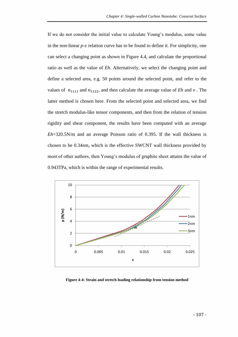
Chapter 4: Single-walled Carbon Nanotube: Cosserat Surface
- 107 -
If we do not consider the initial value to calculate Young’s modulus, some value
in the non-linear p- relation curve has to be found to define it. For simplicity, one
can select a changing point as shown in Figure 4.4, and calculate the proportional
ratio as well as the value of Eh. Alternatively, we select the changing point and
define a selected area, e.g. 50 points around the selected point, and refer to the
values of and , and then calculate the average value of Eh and . The
latter method is chosen here. From the selected point and selected area, we find
the stretch modulus-like tensor components, and then from the relation of tension
rigidity and shear component, the results have been computed with an average
Eh=320.5N/m and an average Poisson ratio of 0.395. If the wall thickness is
chosen to be 0.34nm, which is the effective SWCNT wall thickness provided by
most of other authors, then Young’s modulus of graphite sheet attains the value of
0.943TPa, which is within the range of experimental results.
Figure 4-4: Strain and stretch loading relationship from tension method
0
2
4
6
8
10
0 0.005 0.01 0.015 0.02 0.025
p (
N/m
)
𝜀
1nm
2nm
3nm
Chapter 4: Single-walled Carbon Nanotube: Cosserat Surface
- 108 -
The bending method is sketched in Figure 4.5. A cantilever graphite sheet is under
uniform loading in the third direction. A zigzag SWCNT with L = 8nm, while b is
changing from 1nm to 8nm, is investigated. The loading and displacement
relationship is also non-linear, so we use the same method to select the point and
area and find the dominating bending modulus-like tensor component from the
calculation. With the bending method, and from the relation of the bending
rigidity and tension rigidity, an average Young’s modulus of graphite sheet of
5.526TPa is calculated, with a corresponding average wall thickness of 0.058nm.
A comparison of numerical results for Young’s modulus, wall thickness and
tension rigidity of SWCNTs or graphite sheets with other authors is presented in
Table 4.1.
Figure 4-5: Graphite sheet under bending with uniform loading at the free end
It shows little differences of Young’s modulus and Possion ratio with respect to
the sheet width and sheet aspect ratio b/L in this graphite sheet computation.
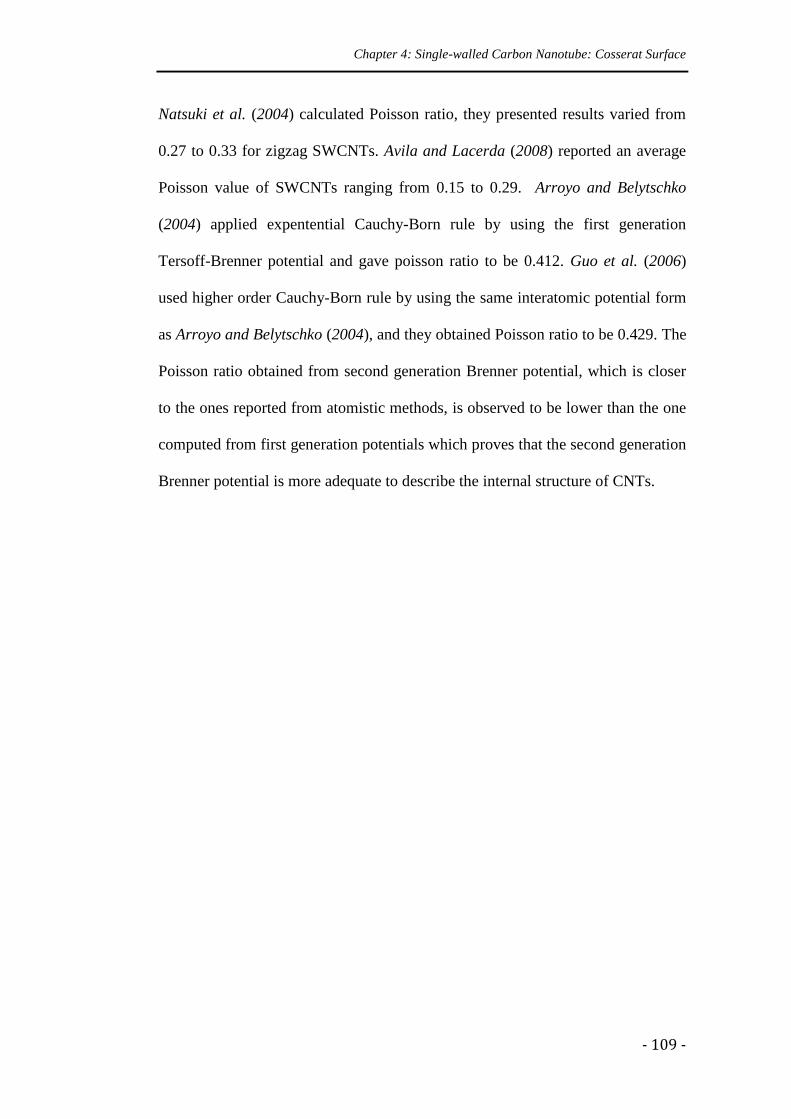
Chapter 4: Single-walled Carbon Nanotube: Cosserat Surface
- 109 -
Natsuki et al. (2004) calculated Poisson ratio, they presented results varied from
0.27 to 0.33 for zigzag SWCNTs. Avila and Lacerda (2008) reported an average
Poisson value of SWCNTs ranging from 0.15 to 0.29. Arroyo and Belytschko
(2004) applied expentential Cauchy-Born rule by using the first generation
Tersoff-Brenner potential and gave poisson ratio to be 0.412. Guo et al. (2006)
used higher order Cauchy-Born rule by using the same interatomic potential form
as Arroyo and Belytschko (2004), and they obtained Poisson ratio to be 0.429. The
Poisson ratio obtained from second generation Brenner potential, which is closer
to the ones reported from atomistic methods, is observed to be lower than the one
computed from first generation potentials which proves that the second generation
Brenner potential is more adequate to describe the internal structure of CNTs.
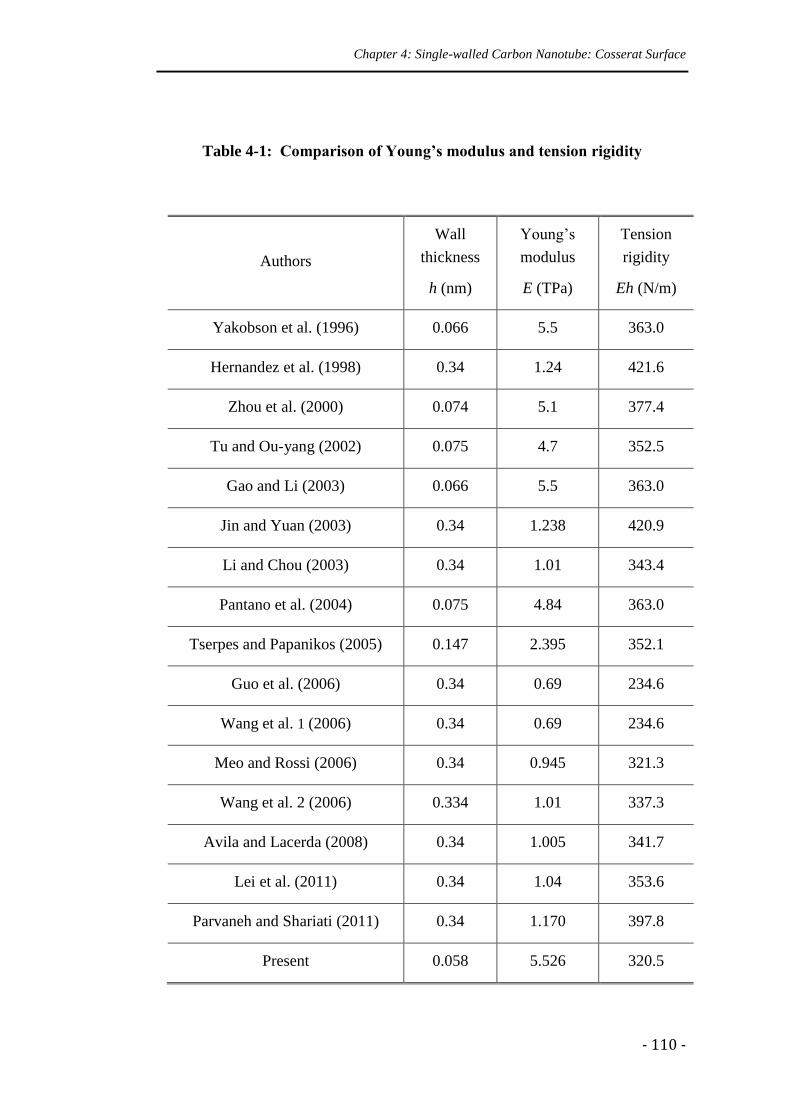
Chapter 4: Single-walled Carbon Nanotube: Cosserat Surface
- 110 -
Table 4-1: Comparison of Young’s modulus and tension rigidity
Authors
Wall
thickness
h (nm)
Young’s
modulus
E (TPa)
Tension
rigidity
Eh (N/m)
Yakobson et al. (1996) 0.066 5.5 363.0
Hernandez et al. (1998) 0.34 1.24 421.6
Zhou et al. (2000) 0.074 5.1 377.4
Tu and Ou-yang (2002) 0.075 4.7 352.5
Gao and Li (2003) 0.066 5.5 363.0
Jin and Yuan (2003) 0.34 1.238 420.9
Li and Chou (2003) 0.34 1.01 343.4
Pantano et al. (2004) 0.075 4.84 363.0
Tserpes and Papanikos (2005) 0.147 2.395 352.1
Guo et al. (2006) 0.34 0.69 234.6
Wang et al. 1 (2006) 0.34 0.69 234.6
Meo and Rossi (2006) 0.34 0.945 321.3
Wang et al. 2 (2006) 0.334 1.01 337.3
Avila and Lacerda (2008) 0.34 1.005 341.7
Lei et al. (2011) 0.34 1.04 353.6
Parvaneh and Shariati (2011) 0.34 1.170 397.8
Present 0.058 5.526 320.5
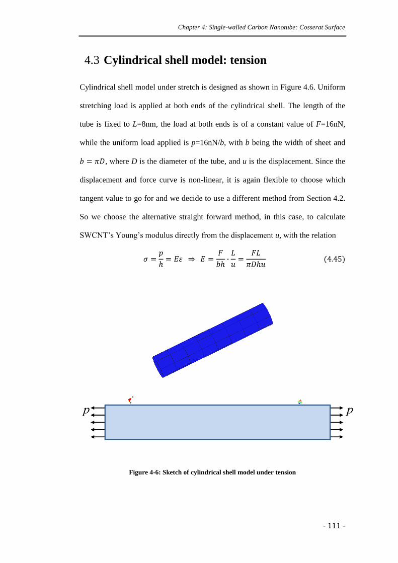
Chapter 4: Single-walled Carbon Nanotube: Cosserat Surface
- 111 -
4.3 Cylindrical shell model: tension
Cylindrical shell model under stretch is designed as shown in Figure 4.6. Uniform
stretching load is applied at both ends of the cylindrical shell. The length of the
tube is fixed to L=8nm, the load at both ends is of a constant value of F=16nN,
while the uniform load applied is p=16nN/b, with b being the width of sheet and
, where D is the diameter of the tube, and u is the displacement. Since the
displacement and force curve is non-linear, it is again flexible to choose which
tangent value to go for and we decide to use a different method from Section 4.2.
So we choose the alternative straight forward method, in this case, to calculate
SWCNT’s Young’s modulus directly from the displacement u, with the relation
Figure 4-6: Sketch of cylindrical shell model under tension
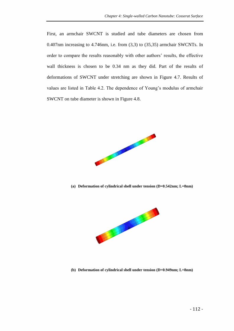
Chapter 4: Single-walled Carbon Nanotube: Cosserat Surface
- 112 -
First, an armchair SWCNT is studied and tube diameters are chosen from
0.407nm increasing to 4.746nm, i.e. from (3,3) to (35,35) armchair SWCNTs. In
order to compare the results reasonably with other authors’ results, the effective
wall thickness is chosen to be 0.34 nm as they did. Part of the results of
deformations of SWCNT under stretching are shown in Figure 4.7. Results of
values are listed in Table 4.2. The dependence of Young’s modulus of armchair
SWCNT on tube diameter is shown in Figure 4.8.
(a) Deformation of cylindrical shell under tension (D=0.542nm; L=8nm)
(b) Deformation of cylindrical shell under tension (D=0.949nm; L=8nm)
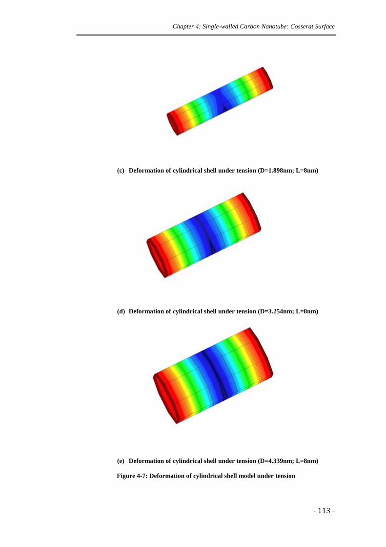
Chapter 4: Single-walled Carbon Nanotube: Cosserat Surface
- 113 -
(c) Deformation of cylindrical shell under tension (D=1.898nm; L=8nm)
(d) Deformation of cylindrical shell under tension (D=3.254nm; L=8nm)
(e) Deformation of cylindrical shell under tension (D=4.339nm; L=8nm)
Figure 4-7: Deformation of cylindrical shell model under tension
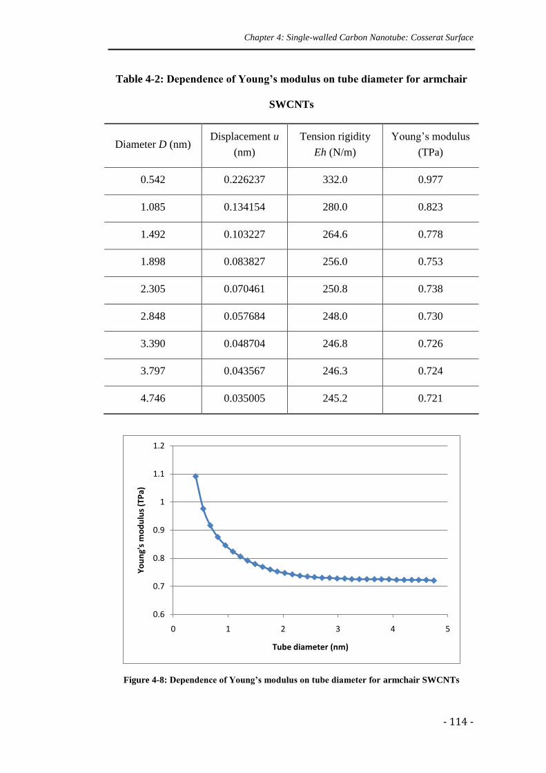
Chapter 4: Single-walled Carbon Nanotube: Cosserat Surface
- 114 -
Table 4-2: Dependence of Young’s modulus on tube diameter for armchair
SWCNTs
Diameter D (nm) Displacement u
(nm)
Tension rigidity
Eh (N/m)
Young’s modulus
(TPa)
0.542 0.226237 332.0 0.977
1.085 0.134154 280.0 0.823
1.492 0.103227 264.6 0.778
1.898 0.083827 256.0 0.753
2.305 0.070461 250.8 0.738
2.848 0.057684 248.0 0.730
3.390 0.048704 246.8 0.726
3.797 0.043567 246.3 0.724
4.746 0.035005 245.2 0.721
Figure 4-8: Dependence of Young’s modulus on tube diameter for armchair SWCNTs
0.6
0.7
0.8
0.9
1
1.1
1.2
0 1 2 3 4 5
Yo
un
g's
mo
du
lus
(TP
a)
Tube diameter (nm)
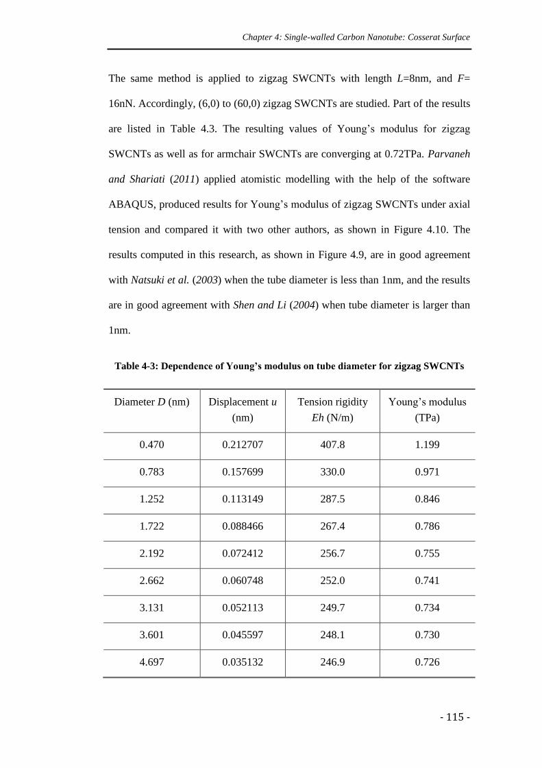
Chapter 4: Single-walled Carbon Nanotube: Cosserat Surface
- 115 -
The same method is applied to zigzag SWCNTs with length L=8nm, and F=
16nN. Accordingly, (6,0) to (60,0) zigzag SWCNTs are studied. Part of the results
are listed in Table 4.3. The resulting values of Young’s modulus for zigzag
SWCNTs as well as for armchair SWCNTs are converging at 0.72TPa. Parvaneh
and Shariati (2011) applied atomistic modelling with the help of the software
ABAQUS, produced results for Young’s modulus of zigzag SWCNTs under axial
tension and compared it with two other authors, as shown in Figure 4.10. The
results computed in this research, as shown in Figure 4.9, are in good agreement
with Natsuki et al. (2003) when the tube diameter is less than 1nm, and the results
are in good agreement with Shen and Li (2004) when tube diameter is larger than
1nm.
Table 4-3: Dependence of Young’s modulus on tube diameter for zigzag SWCNTs
Diameter D (nm) Displacement u
(nm)
Tension rigidity
Eh (N/m)
Young’s modulus
(TPa)
0.470 0.212707 407.8 1.199
0.783 0.157699 330.0 0.971
1.252 0.113149 287.5 0.846
1.722 0.088466 267.4 0.786
2.192 0.072412 256.7 0.755
2.662 0.060748 252.0 0.741
3.131 0.052113 249.7 0.734
3.601 0.045597 248.1 0.730
4.697 0.035132 246.9 0.726
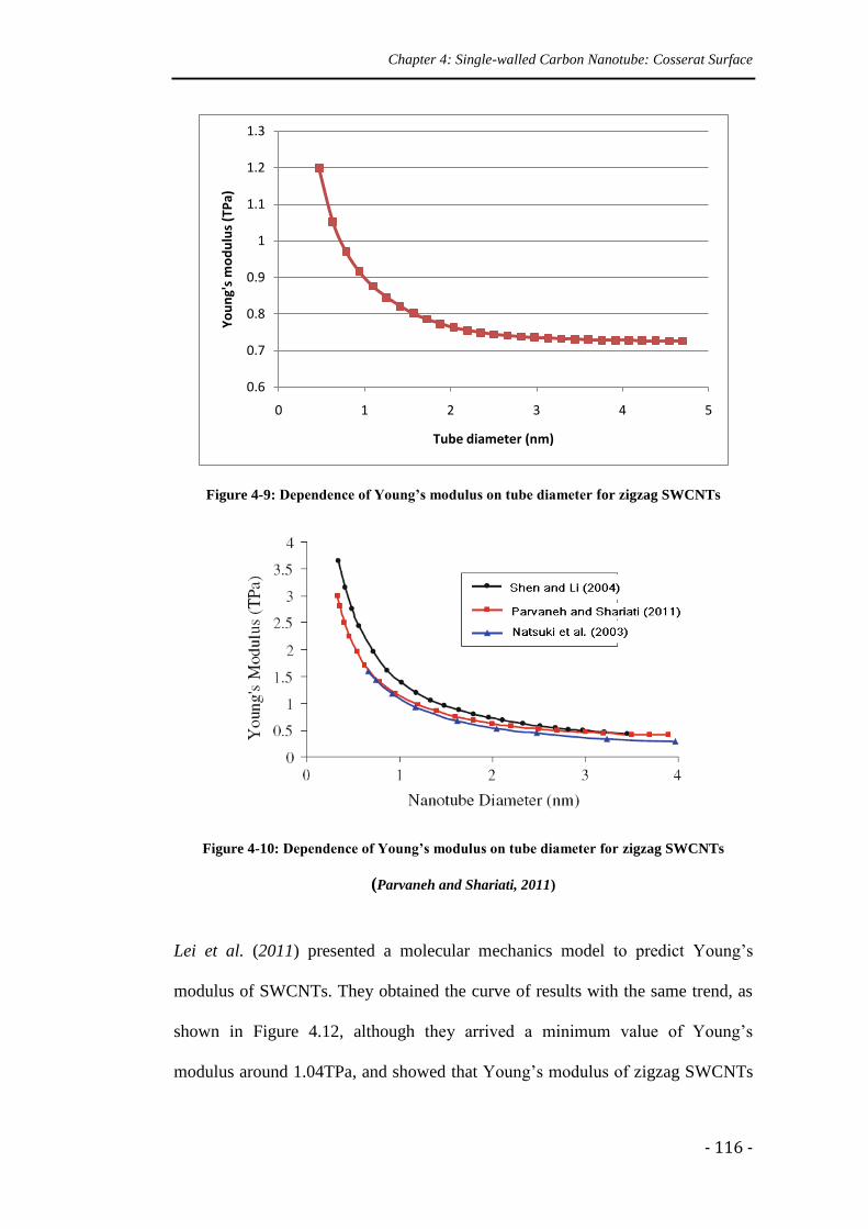
Chapter 4: Single-walled Carbon Nanotube: Cosserat Surface
- 116 -
Figure 4-9: Dependence of Young’s modulus on tube diameter for zigzag SWCNTs
Figure 4-10: Dependence of Young’s modulus on tube diameter for zigzag SWCNTs
(Parvaneh and Shariati, 2011)
Lei et al. (2011) presented a molecular mechanics model to predict Young’s
modulus of SWCNTs. They obtained the curve of results with the same trend, as
shown in Figure 4.12, although they arrived a minimum value of Young’s
modulus around 1.04TPa, and showed that Young’s modulus of zigzag SWCNTs
0.6
0.7
0.8
0.9
1
1.1
1.2
1.3
0 1 2 3 4 5
Yo
un
g's
mo
du
lus
(TP
a)
Tube diameter (nm)
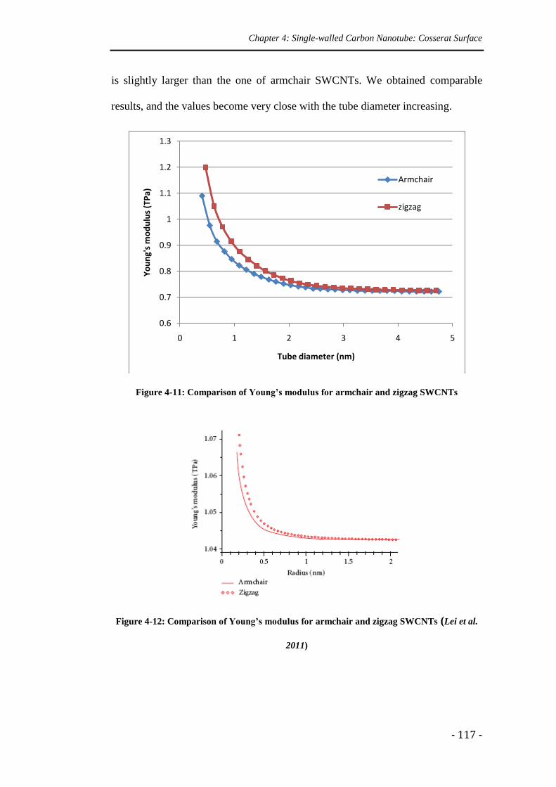
Chapter 4: Single-walled Carbon Nanotube: Cosserat Surface
- 117 -
is slightly larger than the one of armchair SWCNTs. We obtained comparable
results, and the values become very close with the tube diameter increasing.
Figure 4-11: Comparison of Young’s modulus for armchair and zigzag SWCNTs
Figure 4-12: Comparison of Young’s modulus for armchair and zigzag SWCNTs (Lei et al.
2011)
0.6
0.7
0.8
0.9
1
1.1
1.2
1.3
0 1 2 3 4 5
Yo
un
g's
mo
du
lus
(TP
a)
Tube diameter (nm)
Armchair
zigzag
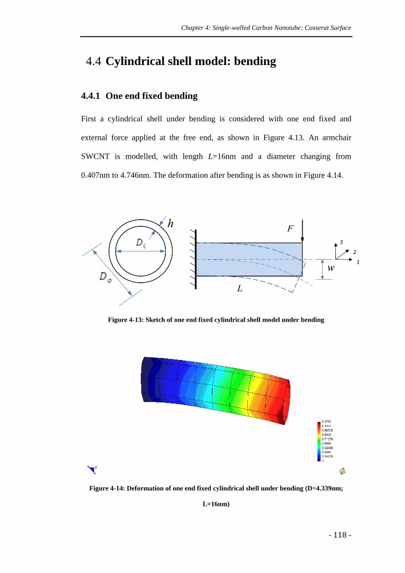
Chapter 4: Single-walled Carbon Nanotube: Cosserat Surface
- 118 -
4.4 Cylindrical shell model: bending
4.4.1 One end fixed bending
First a cylindrical shell under bending is considered with one end fixed and
external force applied at the free end, as shown in Figure 4.13. An armchair
SWCNT is modelled, with length L=16nm and a diameter changing from
0.407nm to 4.746nm. The deformation after bending is as shown in Figure 4.14.
Figure 4-13: Sketch of one end fixed cylindrical shell model under bending
Figure 4-14: Deformation of one end fixed cylindrical shell under bending (D=4.339nm;
L=16nm)
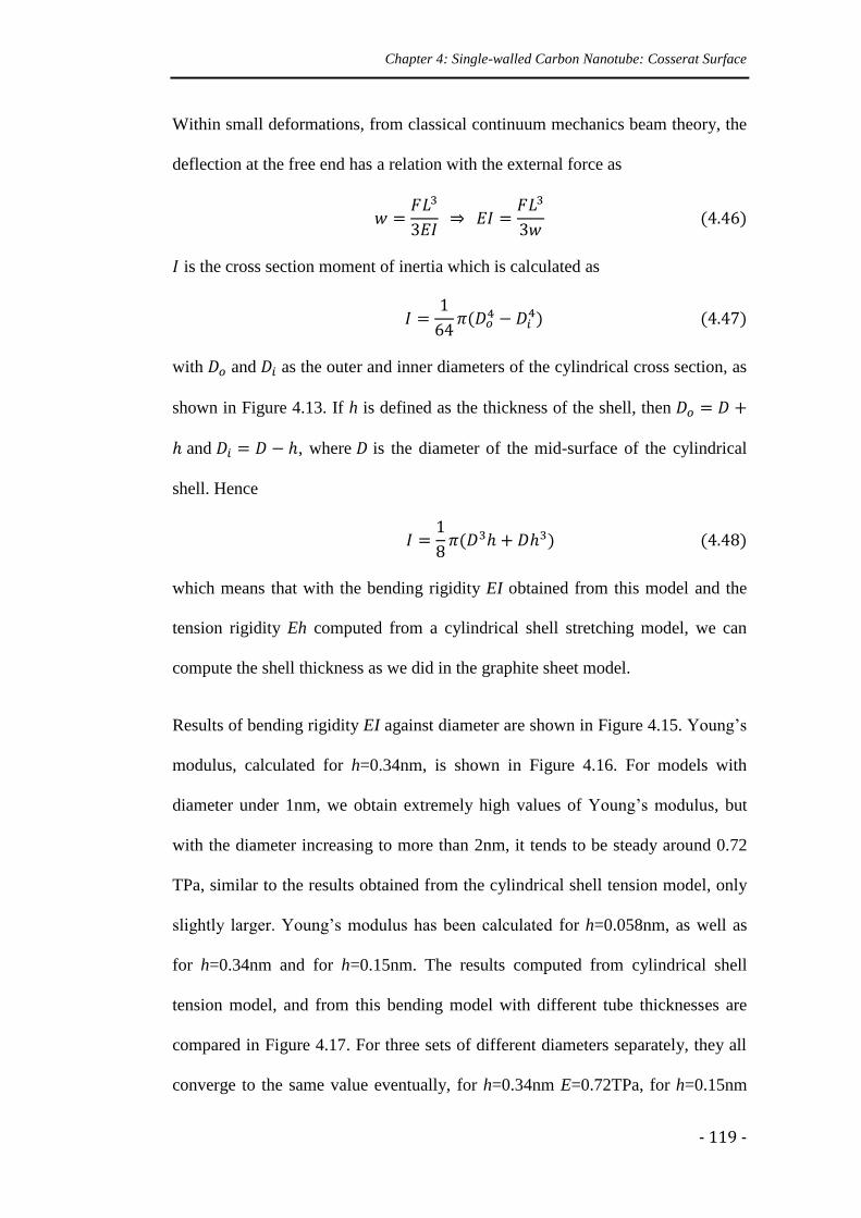
Chapter 4: Single-walled Carbon Nanotube: Cosserat Surface
- 119 -
Within small deformations, from classical continuum mechanics beam theory, the
deflection at the free end has a relation with the external force as
is the cross section moment of inertia which is calculated as
with and as the outer and inner diameters of the cylindrical cross section, as
shown in Figure 4.13. If h is defined as the thickness of the shell, then
and , where is the diameter of the mid-surface of the cylindrical
shell. Hence
which means that with the bending rigidity EI obtained from this model and the
tension rigidity Eh computed from a cylindrical shell stretching model, we can
compute the shell thickness as we did in the graphite sheet model.
Results of bending rigidity EI against diameter are shown in Figure 4.15. Young’s
modulus, calculated for h=0.34nm, is shown in Figure 4.16. For models with
diameter under 1nm, we obtain extremely high values of Young’s modulus, but
with the diameter increasing to more than 2nm, it tends to be steady around 0.72
TPa, similar to the results obtained from the cylindrical shell tension model, only
slightly larger. Young’s modulus has been calculated for h=0.058nm, as well as
for h=0.34nm and for h=0.15nm. The results computed from cylindrical shell
tension model, and from this bending model with different tube thicknesses are
compared in Figure 4.17. For three sets of different diameters separately, they all
converge to the same value eventually, for h=0.34nm E=0.72TPa, for h=0.15nm
Chapter 4: Single-walled Carbon Nanotube: Cosserat Surface
- 120 -
E=1.62TPa, and for h=0.058nm E=4.26TPa. By observing the results, it is
obvious that for predicting Young’s modulus, tension models give much more
stable results compared to bending models.
Figure 4-15: Relationship of bending rigidity against tube diameter (one end fixed bending)
Figure 4-16: Relationship of Young’s modulus against tube diameter for cylindrical shell
mode under bending (one end fixed bending)
0
2
4
6
8
10
12
0 1 2 3 4 5
Be
nd
ing
rigi
dty
(TP
a.n
m^4
)
Tube diameter (nm)
0
1
2
3
4
5
0 1 2 3 4 5
Yo
un
g's
mo
du
lus
(TP
a)
Tube diameter (nm)
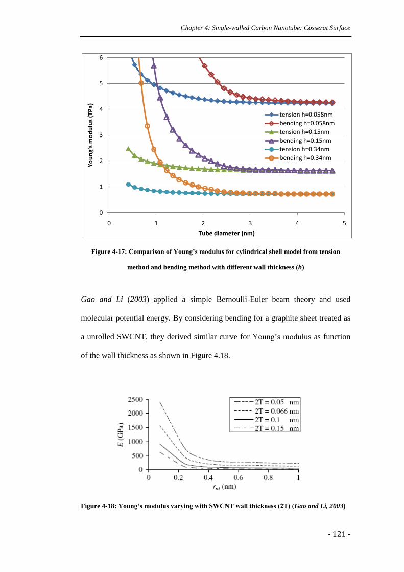
Chapter 4: Single-walled Carbon Nanotube: Cosserat Surface
- 121 -
Figure 4-17: Comparison of Young’s modulus for cylindrical shell model from tension
method and bending method with different wall thickness (h)
Gao and Li (2003) applied a simple Bernoulli-Euler beam theory and used
molecular potential energy. By considering bending for a graphite sheet treated as
a unrolled SWCNT, they derived similar curve for Young’s modulus as function
of the wall thickness as shown in Figure 4.18.
Figure 4-18: Young’s modulus varying with SWCNT wall thickness (2T) (Gao and Li, 2003)
0
1
2
3
4
5
6
0 1 2 3 4 5
Yo
un
g's
mo
du
lus
(TP
a)
Tube diameter (nm)
tension h=0.058nm
bending h=0.058nm
tension h=0.15nm
bending h=0.15nm
tension h=0.34nm
bending h=0.34nm
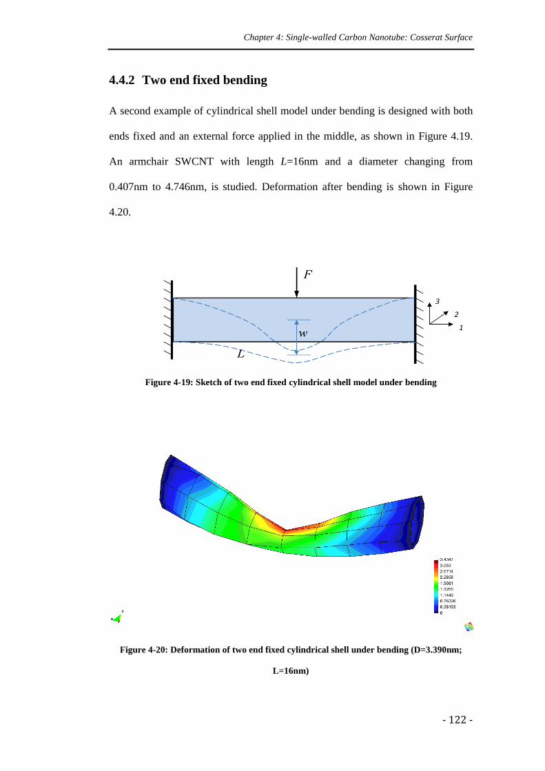
Chapter 4: Single-walled Carbon Nanotube: Cosserat Surface
- 122 -
4.4.2 Two end fixed bending
A second example of cylindrical shell model under bending is designed with both
ends fixed and an external force applied in the middle, as shown in Figure 4.19.
An armchair SWCNT with length L=16nm and a diameter changing from
0.407nm to 4.746nm, is studied. Deformation after bending is shown in Figure
4.20.
Figure 4-19: Sketch of two end fixed cylindrical shell model under bending
Figure 4-20: Deformation of two end fixed cylindrical shell under bending (D=3.390nm;
L=16nm)
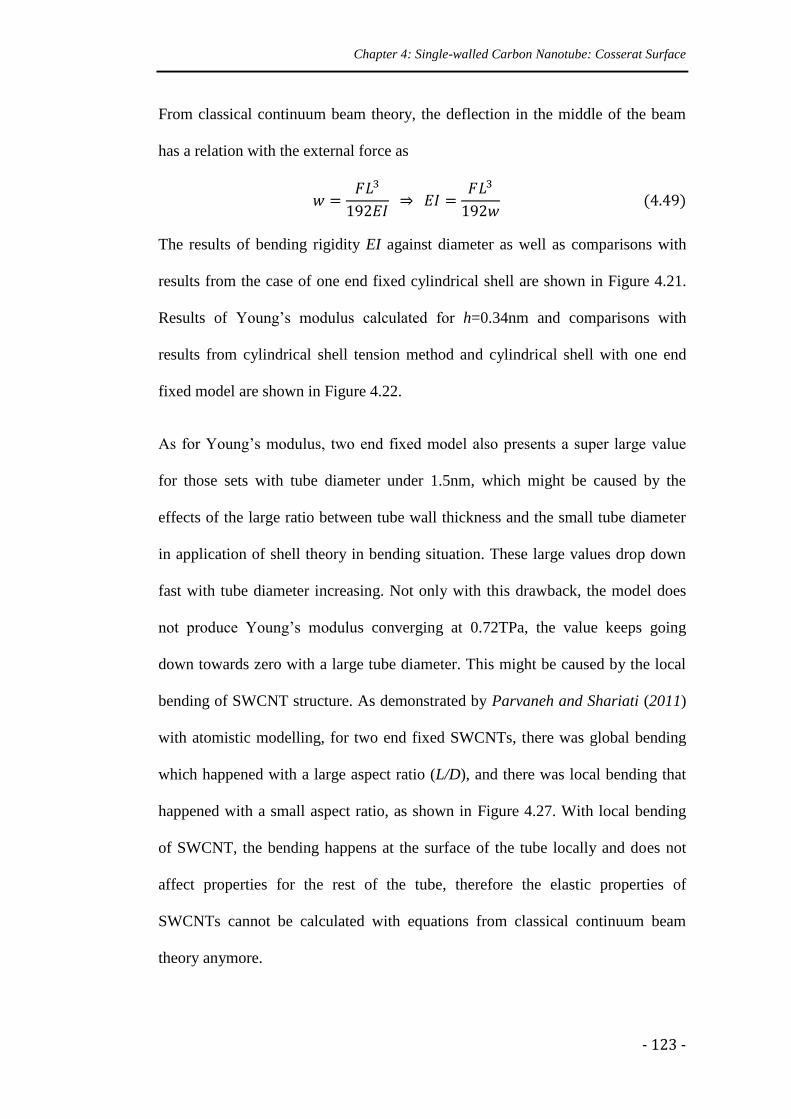
Chapter 4: Single-walled Carbon Nanotube: Cosserat Surface
- 123 -
From classical continuum beam theory, the deflection in the middle of the beam
has a relation with the external force as
The results of bending rigidity EI against diameter as well as comparisons with
results from the case of one end fixed cylindrical shell are shown in Figure 4.21.
Results of Young’s modulus calculated for h=0.34nm and comparisons with
results from cylindrical shell tension method and cylindrical shell with one end
fixed model are shown in Figure 4.22.
As for Young’s modulus, two end fixed model also presents a super large value
for those sets with tube diameter under 1.5nm, which might be caused by the
effects of the large ratio between tube wall thickness and the small tube diameter
in application of shell theory in bending situation. These large values drop down
fast with tube diameter increasing. Not only with this drawback, the model does
not produce Young’s modulus converging at 0.72TPa, the value keeps going
down towards zero with a large tube diameter. This might be caused by the local
bending of SWCNT structure. As demonstrated by Parvaneh and Shariati (2011)
with atomistic modelling, for two end fixed SWCNTs, there was global bending
which happened with a large aspect ratio (L/D), and there was local bending that
happened with a small aspect ratio, as shown in Figure 4.27. With local bending
of SWCNT, the bending happens at the surface of the tube locally and does not
affect properties for the rest of the tube, therefore the elastic properties of
SWCNTs cannot be calculated with equations from classical continuum beam
theory anymore.
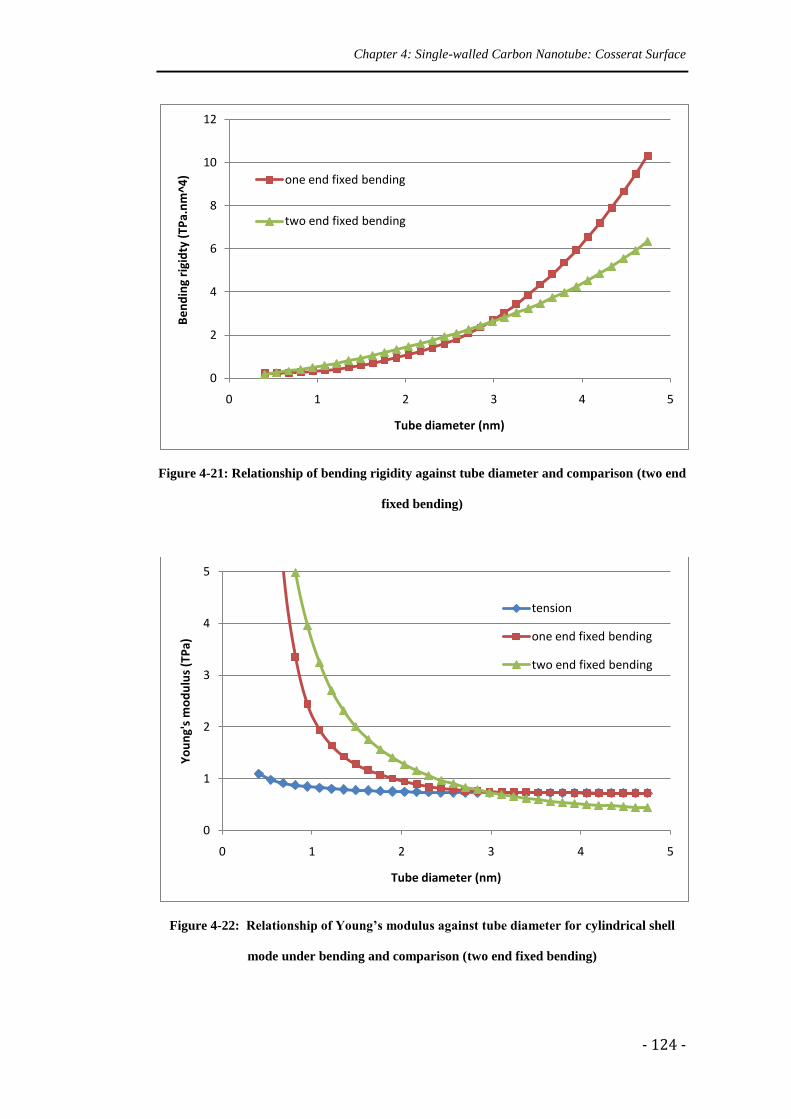
Chapter 4: Single-walled Carbon Nanotube: Cosserat Surface
- 124 -
Figure 4-21: Relationship of bending rigidity against tube diameter and comparison (two end
fixed bending)
Figure 4-22: Relationship of Young’s modulus against tube diameter for cylindrical shell
mode under bending and comparison (two end fixed bending)
0
2
4
6
8
10
12
0 1 2 3 4 5
Be
nd
ing
rigi
dty
(TP
a.n
m^4
)
Tube diameter (nm)
one end fixed bending
two end fixed bending
0
1
2
3
4
5
0 1 2 3 4 5
Yo
un
g's
mo
du
lus
(TP
a)
Tube diameter (nm)
tension
one end fixed bending
two end fixed bending
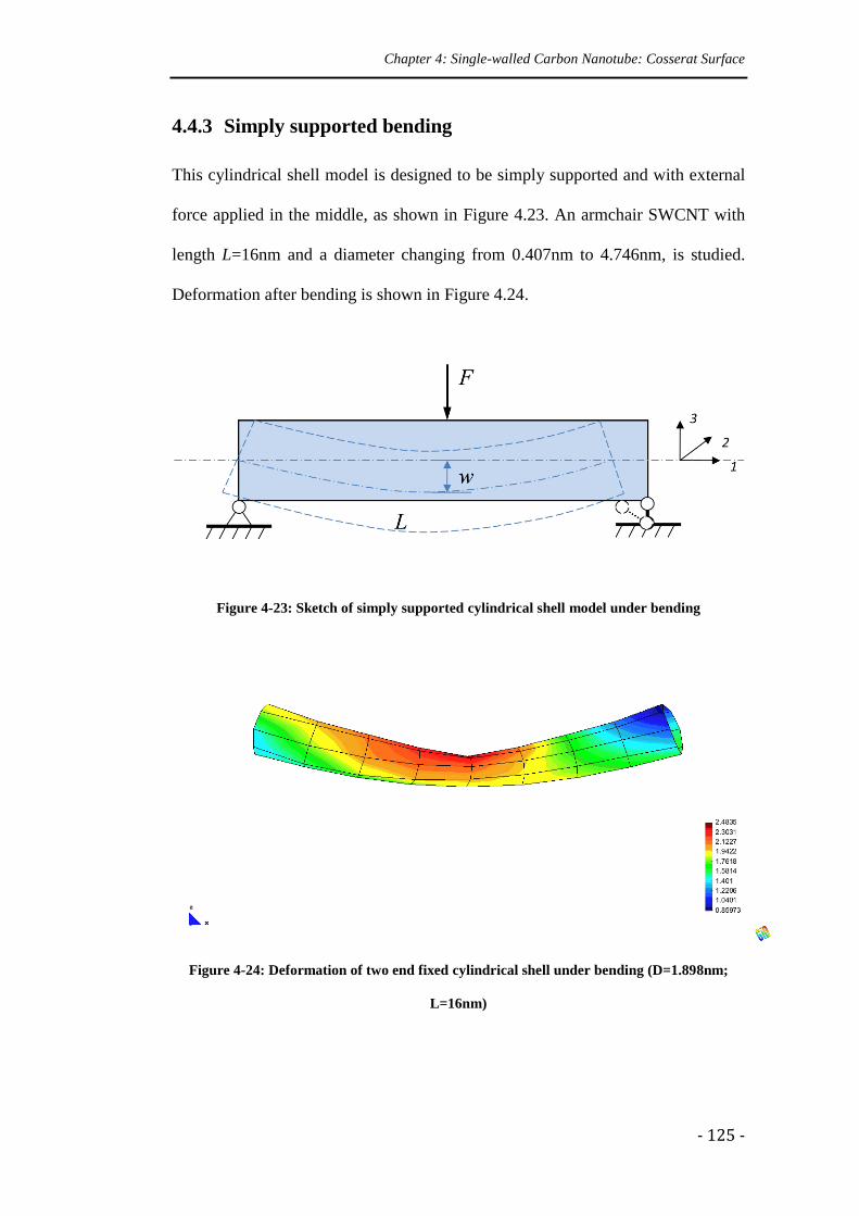
Chapter 4: Single-walled Carbon Nanotube: Cosserat Surface
- 125 -
4.4.3 Simply supported bending
This cylindrical shell model is designed to be simply supported and with external
force applied in the middle, as shown in Figure 4.23. An armchair SWCNT with
length L=16nm and a diameter changing from 0.407nm to 4.746nm, is studied.
Deformation after bending is shown in Figure 4.24.
Figure 4-23: Sketch of simply supported cylindrical shell model under bending
Figure 4-24: Deformation of two end fixed cylindrical shell under bending (D=1.898nm;
L=16nm)
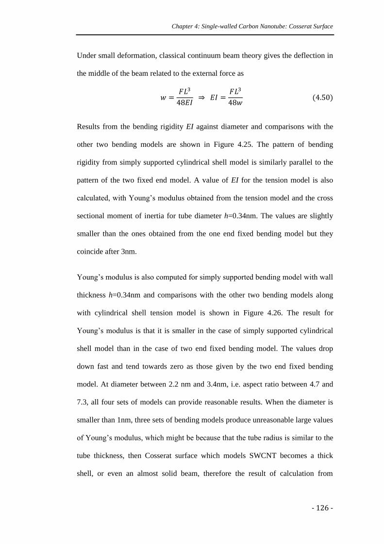
Chapter 4: Single-walled Carbon Nanotube: Cosserat Surface
- 126 -
Under small deformation, classical continuum beam theory gives the deflection in
the middle of the beam related to the external force as
Results from the bending rigidity EI against diameter and comparisons with the
other two bending models are shown in Figure 4.25. The pattern of bending
rigidity from simply supported cylindrical shell model is similarly parallel to the
pattern of the two fixed end model. A value of EI for the tension model is also
calculated, with Young’s modulus obtained from the tension model and the cross
sectional moment of inertia for tube diameter h=0.34nm. The values are slightly
smaller than the ones obtained from the one end fixed bending model but they
coincide after 3nm.
Young’s modulus is also computed for simply supported bending model with wall
thickness h=0.34nm and comparisons with the other two bending models along
with cylindrical shell tension model is shown in Figure 4.26. The result for
Young’s modulus is that it is smaller in the case of simply supported cylindrical
shell model than in the case of two end fixed bending model. The values drop
down fast and tend towards zero as those given by the two end fixed bending
model. At diameter between 2.2 nm and 3.4nm, i.e. aspect ratio between 4.7 and
7.3, all four sets of models can provide reasonable results. When the diameter is
smaller than 1nm, three sets of bending models produce unreasonable large values
of Young’s modulus, which might be because that the tube radius is similar to the
tube thickness, then Cosserat surface which models SWCNT becomes a thick
shell, or even an almost solid beam, therefore the result of calculation from
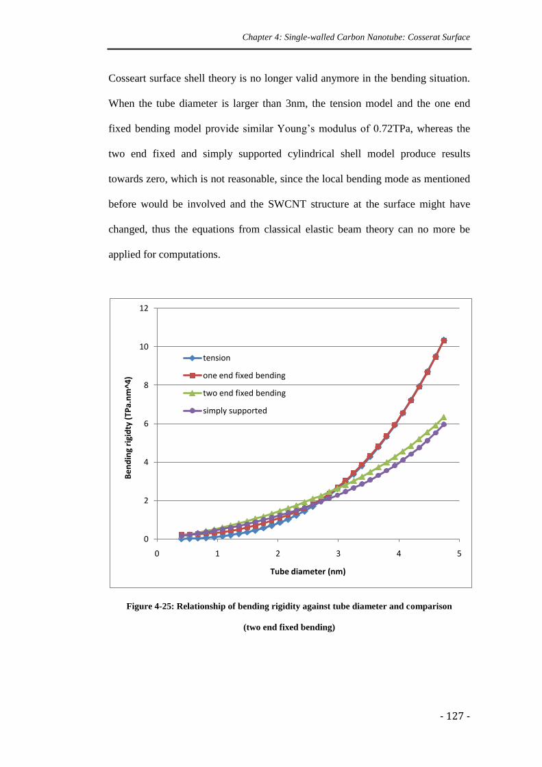
Chapter 4: Single-walled Carbon Nanotube: Cosserat Surface
- 127 -
Cosseart surface shell theory is no longer valid anymore in the bending situation.
When the tube diameter is larger than 3nm, the tension model and the one end
fixed bending model provide similar Young’s modulus of 0.72TPa, whereas the
two end fixed and simply supported cylindrical shell model produce results
towards zero, which is not reasonable, since the local bending mode as mentioned
before would be involved and the SWCNT structure at the surface might have
changed, thus the equations from classical elastic beam theory can no more be
applied for computations.
Figure 4-25: Relationship of bending rigidity against tube diameter and comparison
(two end fixed bending)
0
2
4
6
8
10
12
0 1 2 3 4 5
Be
nd
ing
rigi
dty
(TP
a.n
m^4
)
Tube diameter (nm)
tension
one end fixed bending
two end fixed bending
simply supported
Chapter 4: Single-walled Carbon Nanotube: Cosserat Surface
- 128 -
Figure 4-26: Relationship of Young’s modulus against tube diameter for cylindrical shell
mode under bending and comparison (two end fixed bending)
From all the results shown above, a conclusion is drawn with respect to the
application of shell model for SWCNT in bending, that in case of prediction of
Young’s modulus, direct tension model can provide reasonable results, and one
end fixed bending model can produce similar results with a large tube diameter,
whereas two end fixed and simply supported bending models only can be trusted
within certain range. All three sets of bending models lead to unreasonable large
values of Young’s modulus when the tube diameter is smaller than 1nm, which
indicates that bending models in calculation of Young’s modulus have to be
applied carefully, and a serious consideration should be taken before using
equations from classical beam theory or shell theory because some of the
assumptions may not be valid any more when the wall thickness and the tube
0
1
2
3
4
5
0 1 2 3 4 5
Yo
un
g's
Mo
du
lus
(TP
a)
Tube Diameter (nm)
tension
one end fixed bending
two end fixed bending
simply supported

Chapter 4: Single-walled Carbon Nanotube: Cosserat Surface
- 129 -
diameter are of the same order, or when the inner structure of SWCNT changes
during the calculation.
Parvaneh and Shariati (2011) adopted atomistic modelling and presented four
type of bending deformations with, (a) global bending of one end fixed SWCNT,
(b) local bending of two end fixed SWCNT, (c) global bending of two end fixed
SWCNT, and (d) global bending of simply supported SWCNT. We simulate the
same four types of bending modes, as shown in Figure 4.28.
Figure 4-27: Global bending and local bending of SWCNTs (Parvaneh and Shariati, 2011)
Figure 4-28: Different bending modes of SWCNTs
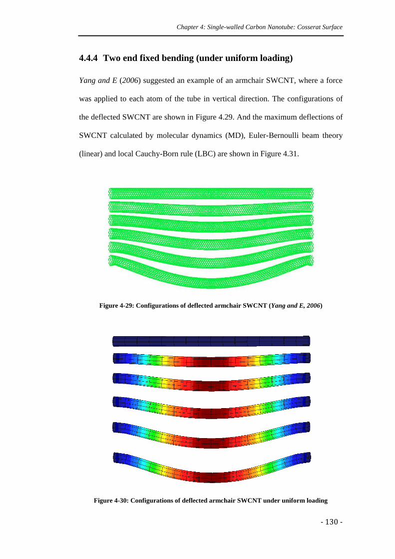
Chapter 4: Single-walled Carbon Nanotube: Cosserat Surface
- 130 -
4.4.4 Two end fixed bending (under uniform loading)
Yang and E (2006) suggested an example of an armchair SWCNT, where a force
was applied to each atom of the tube in vertical direction. The configurations of
the deflected SWCNT are shown in Figure 4.29. And the maximum deflections of
SWCNT calculated by molecular dynamics (MD), Euler-Bernoulli beam theory
(linear) and local Cauchy-Born rule (LBC) are shown in Figure 4.31.
Figure 4-29: Configurations of deflected armchair SWCNT (Yang and E, 2006)
Figure 4-30: Configurations of deflected armchair SWCNT under uniform loading
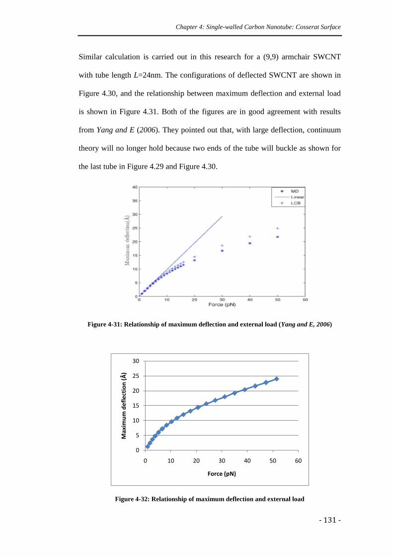
Chapter 4: Single-walled Carbon Nanotube: Cosserat Surface
- 131 -
Similar calculation is carried out in this research for a (9,9) armchair SWCNT
with tube length L=24nm. The configurations of deflected SWCNT are shown in
Figure 4.30, and the relationship between maximum deflection and external load
is shown in Figure 4.31. Both of the figures are in good agreement with results
from Yang and E (2006). They pointed out that, with large deflection, continuum
theory will no longer hold because two ends of the tube will buckle as shown for
the last tube in Figure 4.29 and Figure 4.30.
Figure 4-31: Relationship of maximum deflection and external load (Yang and E, 2006)
Figure 4-32: Relationship of maximum deflection and external load
0
5
10
15
20
25
30
0 10 20 30 40 50 60
Max
imu
m d
efl
ect
ion
(Å
)
Force (pN)
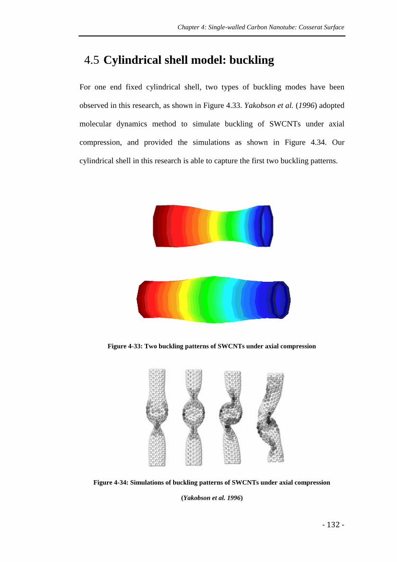
Chapter 4: Single-walled Carbon Nanotube: Cosserat Surface
- 132 -
4.5 Cylindrical shell model: buckling
For one end fixed cylindrical shell, two types of buckling modes have been
observed in this research, as shown in Figure 4.33. Yakobson et al. (1996) adopted
molecular dynamics method to simulate buckling of SWCNTs under axial
compression, and provided the simulations as shown in Figure 4.34. Our
cylindrical shell in this research is able to capture the first two buckling patterns.
Figure 4-33: Two buckling patterns of SWCNTs under axial compression
Figure 4-34: Simulations of buckling patterns of SWCNTs under axial compression
(Yakobson et al. 1996)
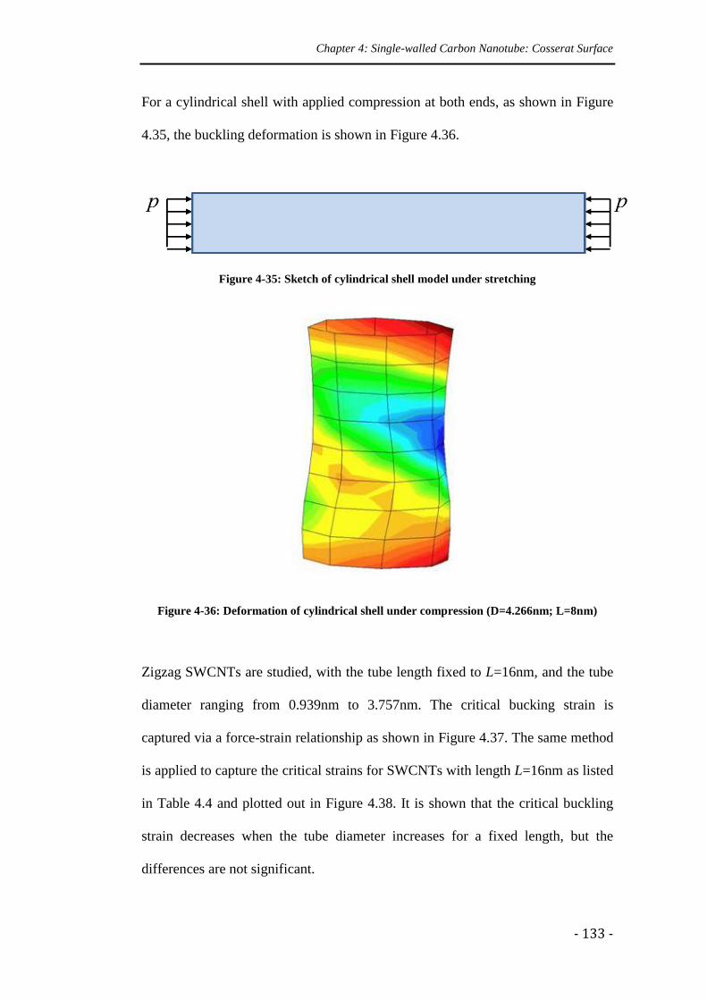
Chapter 4: Single-walled Carbon Nanotube: Cosserat Surface
- 133 -
For a cylindrical shell with applied compression at both ends, as shown in Figure
4.35, the buckling deformation is shown in Figure 4.36.
Figure 4-35: Sketch of cylindrical shell model under stretching
Figure 4-36: Deformation of cylindrical shell under compression (D=4.266nm; L=8nm)
Zigzag SWCNTs are studied, with the tube length fixed to L=16nm, and the tube
diameter ranging from 0.939nm to 3.757nm. The critical bucking strain is
captured via a force-strain relationship as shown in Figure 4.37. The same method
is applied to capture the critical strains for SWCNTs with length L=16nm as listed
in Table 4.4 and plotted out in Figure 4.38. It is shown that the critical buckling
strain decreases when the tube diameter increases for a fixed length, but the
differences are not significant.
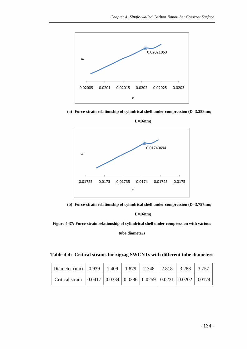
Chapter 4: Single-walled Carbon Nanotube: Cosserat Surface
- 134 -
(a) Force-strain relationship of cylindrical shell under compression (D=3.288nm;
L=16nm)
(b) Force-strain relationship of cylindrical shell under compression (D=3.757nm;
L=16nm)
Figure 4-37: Force-strain relationship of cylindrical shell under compression with various
tube diameters
Table 4-4: Critical strains for zigzag SWCNTs with different tube diameters
Diameter (nm) 0.939 1.409 1.879 2.348 2.818 3.288 3.757
Critical strain 0.0417 0.0334 0.0286 0.0259 0.0231 0.0202 0.0174
0.02021053
0.02005 0.0201 0.02015 0.0202 0.02025 0.0203
F
𝜀
0.01740694
0.01725 0.0173 0.01735 0.0174 0.01745 0.0175
F
𝜀
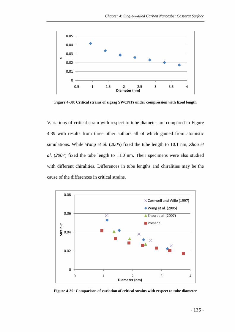
Chapter 4: Single-walled Carbon Nanotube: Cosserat Surface
- 135 -
Figure 4-38: Critical strains of zigzag SWCNTs under compression with fixed length
Variations of critical strain with respect to tube diameter are compared in Figure
4.39 with results from three other authors all of which gained from atomistic
simulations. While Wang et al. (2005) fixed the tube length to 10.1 nm, Zhou et
al. (2007) fixed the tube length to 11.0 nm. Their specimens were also studied
with different chiralities. Differences in tube lengths and chiralities may be the
cause of the differences in critical strains.
Figure 4-39: Comparison of variation of critical strains with respect to tube diameter
0
0.01
0.02
0.03
0.04
0.05
0.5 1 1.5 2 2.5 3 3.5 4
𝜀
Diameter (nm)
0
0.02
0.04
0.06
0.08
0 1 2 3 4
Stra
in 𝜀
Diameter (nm)
Cornwell and Wille (1997)
Wang et al. (2005)
Zhou et al. (2007)
Present
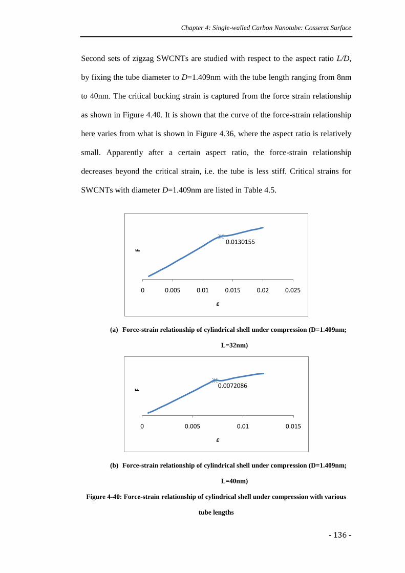
Chapter 4: Single-walled Carbon Nanotube: Cosserat Surface
- 136 -
Second sets of zigzag SWCNTs are studied with respect to the aspect ratio L/D,
by fixing the tube diameter to D=1.409nm with the tube length ranging from 8nm
to 40nm. The critical bucking strain is captured from the force strain relationship
as shown in Figure 4.40. It is shown that the curve of the force-strain relationship
here varies from what is shown in Figure 4.36, where the aspect ratio is relatively
small. Apparently after a certain aspect ratio, the force-strain relationship
decreases beyond the critical strain, i.e. the tube is less stiff. Critical strains for
SWCNTs with diameter D=1.409nm are listed in Table 4.5.
(a) Force-strain relationship of cylindrical shell under compression (D=1.409nm;
L=32nm)
(b) Force-strain relationship of cylindrical shell under compression (D=1.409nm;
L=40nm)
Figure 4-40: Force-strain relationship of cylindrical shell under compression with various
tube lengths
0.0130155
0 0.005 0.01 0.015 0.02 0.025
F
𝜀
0.0072086
0 0.005 0.01 0.015
F
𝜀
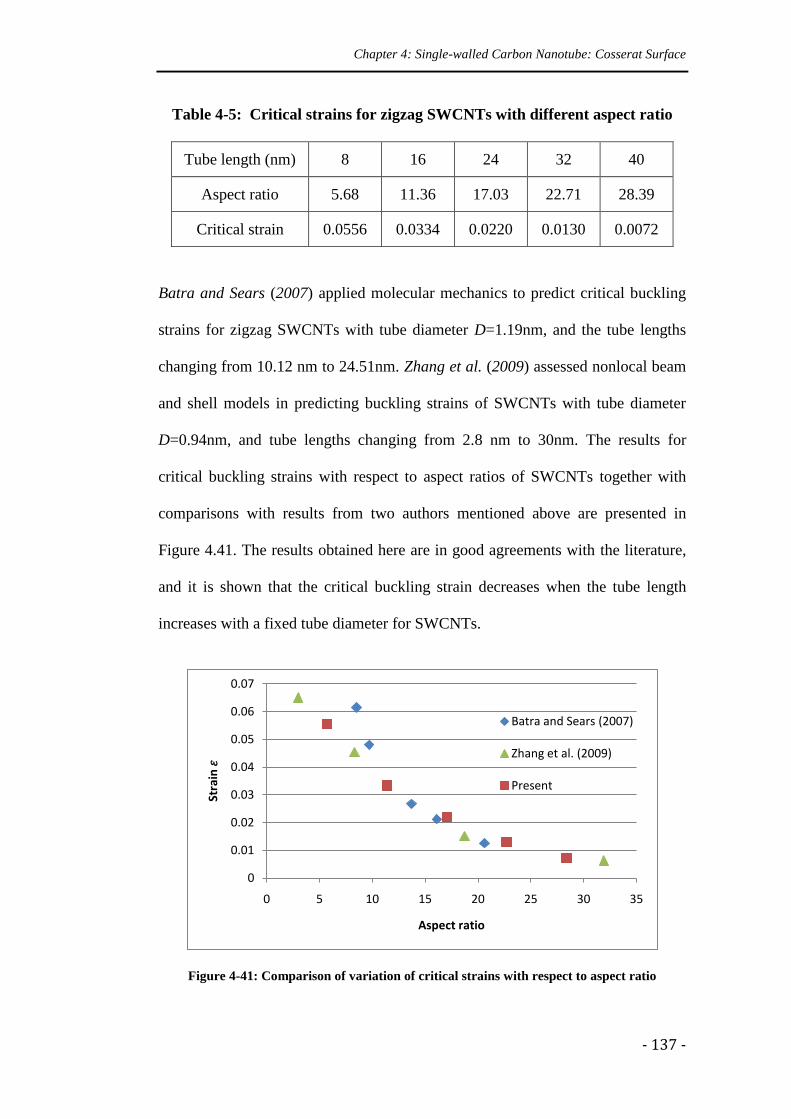
Chapter 4: Single-walled Carbon Nanotube: Cosserat Surface
- 137 -
Table 4-5: Critical strains for zigzag SWCNTs with different aspect ratio
Tube length (nm) 8 16 24 32 40
Aspect ratio 5.68 11.36 17.03 22.71 28.39
Critical strain 0.0556 0.0334 0.0220 0.0130 0.0072
Batra and Sears (2007) applied molecular mechanics to predict critical buckling
strains for zigzag SWCNTs with tube diameter D=1.19nm, and the tube lengths
changing from 10.12 nm to 24.51nm. Zhang et al. (2009) assessed nonlocal beam
and shell models in predicting buckling strains of SWCNTs with tube diameter
D=0.94nm, and tube lengths changing from 2.8 nm to 30nm. The results for
critical buckling strains with respect to aspect ratios of SWCNTs together with
comparisons with results from two authors mentioned above are presented in
Figure 4.41. The results obtained here are in good agreements with the literature,
and it is shown that the critical buckling strain decreases when the tube length
increases with a fixed tube diameter for SWCNTs.
Figure 4-41: Comparison of variation of critical strains with respect to aspect ratio
0
0.01
0.02
0.03
0.04
0.05
0.06
0.07
0 5 10 15 20 25 30 35
Stra
in𝜀
Aspect ratio
Batra and Sears (2007)
Zhang et al. (2009)
Present
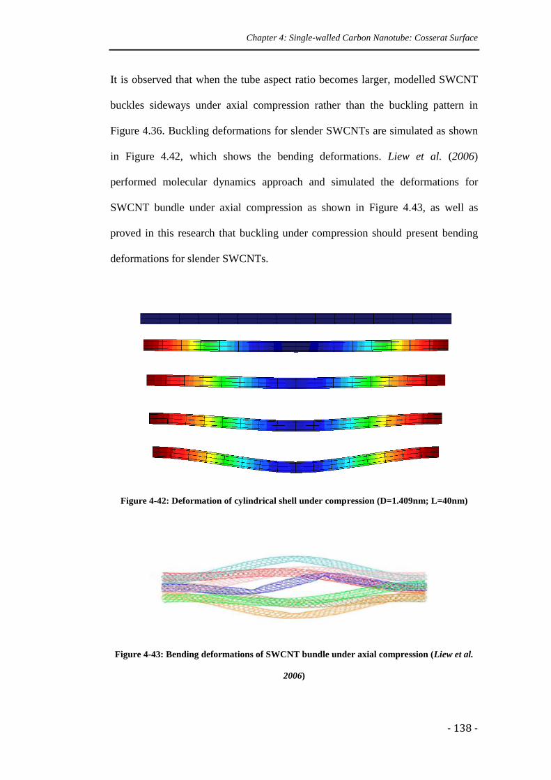
Chapter 4: Single-walled Carbon Nanotube: Cosserat Surface
- 138 -
It is observed that when the tube aspect ratio becomes larger, modelled SWCNT
buckles sideways under axial compression rather than the buckling pattern in
Figure 4.36. Buckling deformations for slender SWCNTs are simulated as shown
in Figure 4.42, which shows the bending deformations. Liew et al. (2006)
performed molecular dynamics approach and simulated the deformations for
SWCNT bundle under axial compression as shown in Figure 4.43, as well as
proved in this research that buckling under compression should present bending
deformations for slender SWCNTs.
Figure 4-42: Deformation of cylindrical shell under compression (D=1.409nm; L=40nm)
Figure 4-43: Bending deformations of SWCNT bundle under axial compression (Liew et al.
2006)
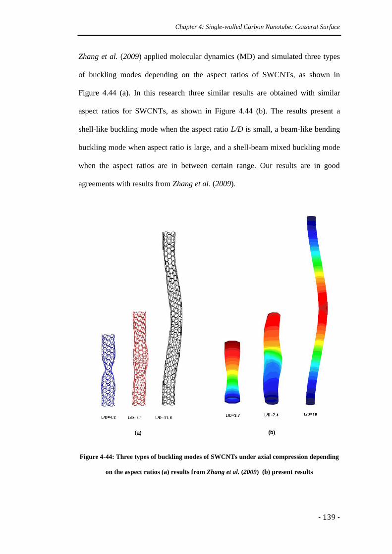
Chapter 4: Single-walled Carbon Nanotube: Cosserat Surface
- 139 -
Zhang et al. (2009) applied molecular dynamics (MD) and simulated three types
of buckling modes depending on the aspect ratios of SWCNTs, as shown in
Figure 4.44 (a). In this research three similar results are obtained with similar
aspect ratios for SWCNTs, as shown in Figure 4.44 (b). The results present a
shell-like buckling mode when the aspect ratio L/D is small, a beam-like bending
buckling mode when aspect ratio is large, and a shell-beam mixed buckling mode
when the aspect ratios are in between certain range. Our results are in good
agreements with results from Zhang et al. (2009).
Figure 4-44: Three types of buckling modes of SWCNTs under axial compression depending
on the aspect ratios (a) results from Zhang et al. (2009) (b) present results
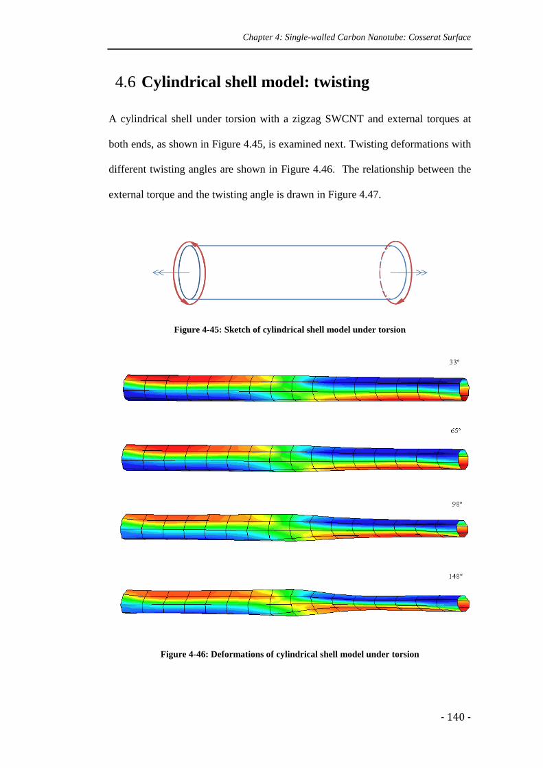
Chapter 4: Single-walled Carbon Nanotube: Cosserat Surface
- 140 -
4.6 Cylindrical shell model: twisting
A cylindrical shell under torsion with a zigzag SWCNT and external torques at
both ends, as shown in Figure 4.45, is examined next. Twisting deformations with
different twisting angles are shown in Figure 4.46. The relationship between the
external torque and the twisting angle is drawn in Figure 4.47.
Figure 4-45: Sketch of cylindrical shell model under torsion
Figure 4-46: Deformations of cylindrical shell model under torsion
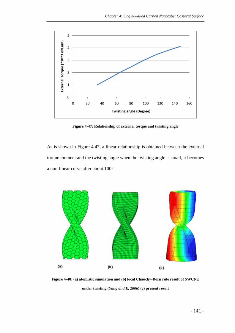
Chapter 4: Single-walled Carbon Nanotube: Cosserat Surface
- 141 -
Figure 4-47: Relationship of external torque and twisting angle
As is shown in Figure 4.47, a linear relationship is obtained between the external
torque moment and the twisting angle when the twisting angle is small, it becomes
a non-linear curve after about 100°.
Figure 4-48: (a) atomistic simulation and (b) local Chauchy-Born rule result of SWCNT
under twisting (Yang and E, 2006) (c) present result
0
1
2
3
4
5
0 20 40 60 80 100 120 140 160
Exte
rnal
To
rqu
e (
*10
^3 n
N.n
m)
Twisting angle (Degree)

Chapter 4: Single-walled Carbon Nanotube: Cosserat Surface
- 142 -
Yang and E (2006) applied local Cauchy-Born rule to simulate SWCNT under
twisting and compared the result with one from atomistic simulation as shown in
Figure 4.48 (a) and (b). With the same dimension and twisting angle studied,
which is a (9,9) armchair SWCNT with tube length L=5nm, and twisting angle
=50°, our result from the Cosserat surface shell theory is shown in Figure 4.48
(c), where it is shown that even with coarse mesh of finite elements, Cosserat
surface-based shell theory can produce reasonable results.
However, since van der Waals forces have not been included in the potential form,
deformations of modelled SWCNT under torsion beyond 148° could not be
captured, because the up and bottom surfaces are twisting towards each other, in
which case, the atoms are close enough and their interactions contribute to the
total energy that cannot be neglected, but they are not neighbours at the reference
configuration whose interactions are not described by bonded energies. Thus, for
large twisting angle deformations, as well as for severe buckling deformations and
severe bending deformations, when two surfaces deform close to each other, van
der Waals forces have to be considered in the potential.
Chapter 5: Conclusions and Discussions
- 143 -
Chapter 5
Conclusions and Discussions
5.1 Summary and conclusions
This research has presented a continuum and atomistic mixing approach to study
the mechanical properties of SWCNTs. Because of the hollow cylindrical shell
structure of SWCNT, it can be modelled as a thin shell, thus Cosserat surface as a
shell model is applied in this research to compute and simulate the mechanical
properties of SWCNTs, for the independent rotation tensor can describe the
rotation field at a micro-level, which as well accounts for a hypothetical curvature
of the deformed surface going beyond the standard Cauchy-Born rule.
Two sets of models are built in this research. As a tool, an atomic chain, which
consists of a series of atoms in a chain, is modelled as a Cosserat curve and
studied through a one-dimensional reduced Cosserat curve theory. For SWCNT,
Chapter 5: Conclusions and Discussions
- 144 -
modelled as a Cosserat surface, the mechanical properties have been studied.
Cauchy-Born rule is applied to link the deformation of the lattice vector at an
atomistic level to the tangent space of the deformation of the system at a
continuum level.
By incorporating the potential form, the stress field and modulus field can be
derived as the first and second derivatives of the potential over the displacement
and rotation fields. For the atomic chain model, interatomic potentials are defined
by a force field, which takes into account bond stretching, bond angle bending and
bond torsion energies. For SWCNT, sophisticated second generation of Brenner
potential is chosen, which contains bond stretching and bond angles as well.
Implementation of the discretization in a finite element approach is accomplished.
The stress fields and the modulus fields are calculated via an iteration procedure
where the displacement and rotation fields are updated. The rotation field is path-
independent updated.
The deformation of an atomic chain under dynamic forces is simulated.
Simulations of the atomic chain model in torsion is also presented, which shows a
vibration mode after vertical instant disturbance, and coiling up mode after
horizontal push. The result matches atomistic simulation of CNTs under torsion
by Yakobson et al. (1996). Simulation of cross section of SWCNTs under bending
is carried on by an atomic ring model. The simulation matches the results for the
deformations of a cross section of SWCNTs under bending from Vodenitcharova
and Zhang (2004) and Kutana and Giapis (2006).
Chapter 5: Conclusions and Discussions
- 145 -
It is shown that the atomic chain model can be used to simulate some behaviour of
SWCNTs, but only provides qualitative results so far. In order to apply atomic
chain model in the use of studying mechanical properties of SWCNTs, the relation
between the structure of the atomic chain and the structure of SWCNT need to be
studied and built numerically, also the potential forms and parameters need to be
modified to provide quantitatively accurate results. Despite of the fact that a lot of
improvements need to be made for atomic chain models to have physical
meanings, 1-D atomic chain as a Cosserat curve model presents a fine preparation
for further use of Cosserat surface to model and simulate SWCNTs.
For the study of SWCNTs, configuration formulas are established in addition to
introducing an inner displacement because of the non-centrosymmetric hexagonal
structure of a carbon cell. The mechanical properties of SWCNTs are then
predicted via the finite element method.
Young’s modulus and Poisson ratio are predicted for a zigzag SWCNT. With
tension method, an average tension rigidity of 320.5 N/m and an average Poisson
ratio of 0.395 are obtained, which are in good agreement with the literature. By
the bending method, the effective wall thickness of SWCNT is computed as
0.058nm, which leads to an average of Young’s modulus being 5.526TPa.
For SWCNT under stretching, results are gained that Young’s modulus is
decreasing with the increase of tube diameter. By applying wall thickness as
0.34nm, Young’s modulus is converging at 0.72TPa, by which the result of
dependence of Young’s modulus on tube diameter for zigzag SWCNTs is in good
agreement with results from Natsuki et al. (2003), Shen and Li (2004) and
Chapter 5: Conclusions and Discussions
- 146 -
Parvaneh and Shariati (2011). And it is shown that Young’s modulus of SWCNT
with zigzag structure is slightly larger than that of the armchair one, which is
agreed with the results from Lei et al. (2011).
SWCNTs under bending are simulated in three situations: one end fixed bending,
two end fixed bending and two end simply supported bending. The results have
shown that, as for the prediction of Young’s modulus of SWCNT, bending
methods have to be considered carefully, although one end fixed model can
predict similar results with cylindrical shell under tension when the tube diameter
is large enough, all three sets of bending models provide extremely large values of
Young’s modulus when the tube diameter is small, while the two end fixed model
and the two end simply supported model provide values of Young’s modulus
towards zero when the tube diameter is large. Demonstration of non-local bending
and local bending of SWCNTs are also presented.
SWCNTs under compression are simulated. Critical buckling strains have been
captured by reading the force and strain relationship. The results show that, for a
fixed tube length, critical buckling strain decreases with the tube diameter
increasing. And for a fixed tube diameter, critical buckling strain decreases when
the tube length increases. Results are in good agreement with the literature.
Twisting deformations of SWCNTs are also simulated, and a non-linear behaviour
after twisting angle of 100° is captured.
Chapter 5: Conclusions and Discussions
- 147 -
5.2 Discussions and recommendations
Shell models have been applied widely to model SWCNTs (Tu and Ou-yang,
2002, Pantano et al. 2004, Arroyo and Belytschko, 2002, 2003, 2004). But it is
hard to define Young’s modulus and shell thickness in a classical linear elastic
shell theory, where the wall thickness has been calculated from 0.066nm to
0.34nm as demonstrated in Table 4.1. In this case, Cosserat surface presented a
great advantage by avoiding the shell thickness as well as Young’s modulus itself,
but linking the tension and bending rigidities directly to interatomic potentials.
The link between atomistic deformations and continuum deformations is provided
by the Cauchy-Born rule. However, the drawback of the Cauchy-Born rule for
SWCNTs is that the deformation map maps the deformed lattice vector onto the
tangent plane of the deformed surface, which does not matter for bulk material but
has significant effects on a thin surface material such as SWCNTs, especially
when a large curvature is involved. Therefore, modifications need to be made to
the Cauchy-Born rule for its application to study SWCNTs, in which aspect,
Cosserat surface as a shell model makes perfect compatibility with the standard
Cauchy-Born rule, since in a Cosserat surface-based shell theory, a displacement
field-independent rotation tensor is introduced that describes the curvature at each
point of the surface, which relates the rotation field to the inner structure of the
surface, i.e. at a micro-level. Therefore, the Cauchy-Born rule describes the
tangent map, while the change of curvature of the deformed surface is captured by
rotation tensor which describes the micro-level rotation map.
Chapter 5: Conclusions and Discussions
- 148 -
An ideal potential model should be able to accurately describe the interactions
among atoms in a SWCNT. How accurate the empirical potentials are defined
plays a very important role on how well the results come out, because different
potential models, or even different sets of parameters in the potential form can
lead to big differences in the results, which was also pointed out by Wang et al.
(2006) and Wu et al. (2008).
In this research, we adopt interatomic potential forms based on a force field to
describe potentials for the atomic chain, which is of advantage since the atomic
chain model consists of a series of atoms, and so a force field defines all the
interactions between atoms, except that the C-C bond atomic chain model has not
been given a physical explanation, since C-C bonds have hexagonal structure in
the SWCNT structure rather than a straight line. However, an atomic chain model
presents various behaviours that are similar to SWCNT’s behaviours, so if the
relation between an atomic chain and SWCNT, or any other similar atomic
structures, can be studied and constructed and if the potential forms can be
reformulated, atomic chain models could be very handy for simulation of string-
like nanostructures.
Cosserat surface as a shell model has been built to simulate SWCNTs. Second
generation Brenner potential formulation is adopted. The first generation of
Tersoff-Brenner potential has been applied widely by previous researchers, in
most cases produced an opposite trend of the results, as shown in Figure 1.2 and
Figure 1.4, and also as shown in results from Arroyo and Belytschko (2004),
where Young’s modulus of SWCNT increases with the tube diameter increasing
and converging at around 0.69TPa. Second generation Brenner potential has not
Chapter 5: Conclusions and Discussions
- 149 -
been used as much, since the formulation is new and the adjustments make the
potential forms much more complicated, and atoms from second layer in the
neighbourhood are involved in the calculation. Extra potential terms which
describe shear effects and atom spin effects are added to assure the non-
singularity of the tangent modulus.
Most researches in recent years have applied atomistic potential forms from force
field, and built C-C bonds as a beam, rod or spring, and built-in the constitutive
law into commercial software, such as ANSYS or ABAQUS (Avila and Lacerda,
2008; Dun et al. 2010; Shokrieh and Rafiee, 2010; Parvaneh and Shariati, 2011).
The results received in this research are in good agreement with the results from
these atomistic simulations based on force field potentials. And the results of
buckling patterns and twisting patterns are still in agreement with previous
researchers who applied first generation Tersoff-Brenner potential forms, because
the change of potential forms did affect the results of Young’s modulus, but it
didn’t affect the bending, buckling and twisting patterns.
Young’s modulus and Poisson ratio has been obtained from tension and bending
methods for graphite sheet. Because the force displacement relationship Cosserat
surface-based shell theory provides is non-linear, it is rather flexible and
subjective to decide what value to go for to calculate Young’s modulus of graphite
sheet. Assume wall thickness is 0.34nm, if initial value is selected from the results
of graphite sheet tension that leads to a Young’s modulus of 0.706TPa. In this
research, we go for the other method of selecting a changing point and an area
around it to calculate an average value, in which case, it arrives an average
Young’s modulus of 0.943TPa for wall thickness 0.34nm, which is in good
Chapter 5: Conclusions and Discussions
- 150 -
agreement with the experimental results. But still, the definition of selected area is
subjective and then the result may vary from time to time.
Therefore, we decide to use another method which is straight forward to calculate
Young’s modulus for SWCNTs modelled by cylindrical shells, where we adopt
the equations from classical elastic beam theory which build a relation between
external forces and the final deflection. In which way, results of Young’s modulus
for SWCNTs obtained from the tension model are still within the range, but
results from the bending models become unreasonable. One end fixed bending
model can still provide similar results with the tension model when tube diameter
is large, while the two end fixed and the two end simply supported models result
in a Young’s modulus value towards zero when tube diameter becomes large. And
all three sets of bending models produce extremely high values of Young’s
modulus when the tube diameter is small. All these errors might be caused by two
reasons, either when the tube diameter is small enough that the size of tube
diameter and the size of tube wall thickness is similar, in which case, shell theory
cannot be applied anymore, or when the tube diameter is large enough that there is
only deformations on the surface rather than the whole system, in which case, the
equations from classical beam theory are not valid anymore. To sum up, by
applying continuum theory in calculating properties of SWCNTs, the size effects
have to be considered, and the assumptions have to be used carefully because they
may not be valid anymore in some situations, even in elastic cases.
The whole calculation, except few cases, has been carried on by 8⤫8 element
models, which includes 486 degrees of freedom for graphite sheet and only 432
degrees of freedom for cylindrical shell model, which already provide reasonable
Chapter 5: Conclusions and Discussions
- 151 -
results with good agreements with the literature. If the calculation is carried on by
more elements, i.e. finer meshes, it should be able to catch more detailed
information about the behaviour of SWCNTs.
Van der Waals force interactions have not been considered in either atomic chain
model or cylindrical shell model, which contributes to the non-bonded energies in
the total potential forms. It describes the interatomic reactions between two atoms
that are not bonded within certain range in SWCNT case, which can normally be
neglected when the bonded energies dominate the total energy, as is considered in
this research. However, non-bonded energy cannot be ignored in the study of
MWCNTs, as van der Waals forces contributes to the interactions between the
layers of CNTs, in which case we need to add van der Waals force energy, which
is normally described by Lennard-Jones potential, if we want to do further
research about MWCNTs. Van der Waals force should also not be neglected when
SWCNT is studied under severe deformation, like when the tube is under severe
bending that two ends move towards each other, the atoms from two surfaces
become close enough but bonded energy cannot define the interactions of the
close non-bonded atoms which can only be described by van der Waals force, or
when tube is under large torsion deformation, van der Waals force also needs to
be included for the atoms on two close surfaces under twisting.
Future work will focus on:
1. Check the validation of the potential forms, possible modifications will be
made to fit the potential in an atomistic level. Neglected terms need to be
checked if they would make much differences for the results. Applications
Chapter 5: Conclusions and Discussions
- 152 -
of other empirical potentials will be used and compared to find an
optimized solution.
2. Van der Waals force interactions should be considered based on Lennard-
Jones 6-12 expressions, in order to study more complicated deformations
of SWCNTs, or possibly MWCNTs. In this case, third and forth buckling
patterns, severe local bending, and large angle twisting deformations for
SWCNTs will then be simulated.
3. More elements with finer meshes need to be applied to provide more
detailed information. Nine-node elements will be used to study tensile
strength, buckling failure, fracture of CNTs, or other aspects involving
stress concentrating.
4. Quantitative properties obtained from cylindrical shell models for CNTs
will be used to calculate parameters in the potential forms for atomic chain
model, in order to check if an easy 1-D Cosserat curve model can produce
reasonable results in simulating CNTs’ behaviours.
References
- 153 -
References
Ajayan, P. M., Zhou, O.Z. (2001) Applications of carbon nanotubes, Carbon
Nanotubes, 80, 391-425.
Arroyo, M., Belytschko, T. (2002) An atomistic-based finite deformation
membrane for single layer crystalline films. Journal of the Mechanics and
Physics of Solids, 50, 1941-1977.
Arroyo, M., Belytschko, T. (2003) A finite deformation membrane based on inter-
atomic potentials for the transverse mechanics of nanotubes. Mechanics of
Materials, 35 (3-6), 193-215.
Arroyo, M., Belytschko, T. (2004) Finite crystal elasticity of carbon nanotubes
based on the exponential Cauchy-Born rule. Physical Review B, 69:115415.
Arroyo, M., Belytschko, T. (2004) Finite element methods for the non-linear
mechanics of crystalline sheets and nanotubes, International Journal for
Numerical Methods in Engineering, 59, 419-456.
Avila, A.F., Lacerda, G.S. (2008) Molecular mechanics applied to single-walled
carbon nanotubes. Materials Research, Vol. 11, No. 3, 325-333.
References
- 154 -
Avouris, P. (2002) Carbon Nanotube Electronics. Chemical Physics, 281, 429-
445.
Bao, W.X., Zhu, C.C., Cui, W.Z. (2004) Simulation of Young's modulus of
single-walled carbon nanotubes by molecular dynamics. Physica B:
Condensed Matter, 352 (1-4), 156-163.
Batra, R.C., Sears, A. (2007) Continuum models of multi-walled carbon
nanotubes. Int. J. Solids Struct., 44, 7577-7596.
Baughman, R. H., Zakhidov, A. A., Heer, W. A. (2002) Carbon nanotubes-the
route toward applications. Science, 297, 787-792.
Belytschko, T., Xiao, S.P., Schatz, G.C., Ruoff, R.S. (2002) Atomistic simulations
of nanotube fracture, Phys Rev B, 65, 235430.
Bertoni, G., Calmels, L. (2006) First-principles calculation of the electronic
structure and energy loss near edge spectra of chiral carbon nanotubes.
Micron, 37 (5), 486-491.
Brenner, D.W. (1989) Tersoff-type Potentials for Carbon, Hydrogen and
Oxygen", Mat. Res. Soc. Symp. Proc. 141, 59-64.
Brenner, D.W., Shenderova, O.A., Harrison, J.A., Stuart, S.J., Ni, B., Sinnott, S.B.
(2002) A second-generation reactive empirical bond order (REBO) potential
energy expression for hydrocarbons. J. Phys.: Condens. Matter 14, 783–802.
Buongiorno-Nardelli, M., Yakobson, B.I., Bernhold, J. (1998) Mechanism of
strain release in carbon nanotubes. Phys. Rev. Lett. 81, 4656; Phys. Rev. B. 57,
4277.
Cai, J., Bie, R. F., Tan, X. M., Lu, C. (2004) Application of the tight-binding
method to the elastic modulus of C60 and carbon nanotube. Physica B:
Condensed Matter, 344 (1-4), 99-102.
References
- 155 -
Chandraseker, K., Mukherjee, S., Mukherjee, Y. X. (2006) Modifications to the
Cauchy–Born rule: Applications in the deformation of single-walled carbon
nanotubes. International Journal of Solids and Structures, 43 (22-23), 7128-
7144.
Chang, T., Gao, H. (2003) Size-dependent elastic properties of a single-walled
carbon nanotube via a molecular mechanics model. Journal of the Mechanics
and Physics of Solids, 51, 1059-1074.
Cornwell, C.F., Wille, L.T. (1997) Proposed growth mechanism of single-walled
carbon nanotubes. Chemical Physics Letters 278, 262-266.
Dai, H., Hafner, J. H., Rinzler, A. G., Colbert, D. T., Smalley, R. E.(1996)
Nanotubes as nanoprobes in scanning probe microscopy. Nature, 384, 147-
150.
Damnjanovic, M., Milosevic, I., Vukovic, T., Sredanovic, R. (1999) Full
Symmetry, Optical Activity and Potentials of Single- and Multi-wall
Nanotubes, Phys. Rev. B. 60, 2728-2739.
Dresselhaus, M.S., Dresselhaus, G., Eklund, P. C. (1996) Science of Fullerenes
and Carbon Nanotubes. Academic Press Inc.
Duan, W. H., Wang, Q., Wang, Q., Liew, K. (2010) Modelling the Instability of
Carbon Nanotubes: From Continuum Mechanics to Molecular Dynamics.
Journal of Nanotechnology in Engineering and Medicine. Vol. 1, 011001-10.
Endo, M., Hayashi, T., Kim, Y.A., Muramatsu, H. (2006) Development and
application of carbon nanotubes. Japanese Journal of Applied Physics, 45
(6A), 4883–4892.
References
- 156 -
Gao, X. L., Li, K. (2003) Finite deformation continuum model for single-walled
carbon nanotubes. International Journal of Solids and Structures, 40(26),
7329-7337.
Govindjee, S., Sackman, J. L. (1999) On the use of continuum mechanics to
estimate the properties of nanotubes. Solid State Communications, 110 (4),
227-230.
Guo, X., Wang, J. B., Zhang, H.W. (2006) Mechanical properties of single-walled
carbon nanotubes based on higher order Cauchy–Born rule. International
Journal of Solids and Structures, 43 (5), 1276-1290.
Haefner, J., Sachse, F.B., Sansour, C., Seeman, G. (2002) Hyperelastic description
of elastomechanic properties of the heart: A new material law and its
application. Biomedical Engineering -Supplement, 47(6), 770-773.
Hall, B.C. (2003) Lie Groups, Lie Algebras, and Representations: An Elementary
Introduction, Springer, ISBN 0-387-40122-9.
Harris, P. J. F. (2009) Carbon Nanotube Science: Synthesis, Properties and
Applications. Cambridge University Press.
He, X. Q., Kitipornchai, S., Wang, C. M., Liew, K. M. (2005) Modelling of van
der Waals force for infinitesimal deformation of multi-walled carbon
nanotubes treated as cylindrical shells. International Journal of Solids and
Structures, 42 (23), 6032-6047.
He, X. Q., Kitipornchai, S., Liew, S. (2005) Buckling analysis of multi-walled
carbon nanotubes: a continuum model accounting for van der Waals
interaction. Journal of the Mechanics and Physics of Solids, 53 (2), 303-326.
Hernandez, E., Goze, C., Bernier, P. Rubio, A. (1998) Elastic properties of C and
BxCyNz Composite Nanotubes. Phys. Rev. Lett. 80, 4502–4505.
References
- 157 -
Hertel, T., Martel, R., Avouris, P. (1998) Manipulation of carbon nanotubes and
their Interaction with Surfaces. J. Phys. Chem. B 102, 910-915.
Hone, J., Llaguno, M. C., Biercuk, M. J., Johnson, A. T., Batlogg, B., Benes, Z.,
Fischer, J. E. (2002) Thermal properties of carbon nanotubes and nanotube-
based materials. Appl. Phys. A, 74, 339–343.
Huang, Y., Wu, J., Hwang, K. C. (2006) Thickness of graphene and single-wall
carbon nanotubes. Physical Review B, 74, 245413.
Huhtala, M., Kuronen, A., Kaski, K. (2002) Carbon nanotubes under bending
strain. Mat. Res. Soc. Symp. Proc. Vol. 706.
Iijima, S. (1991) Helical microtubules of graphitic carbon. Nature 354, 56–58.
Ito, T., Nishidate, K., Baba, M., Hasegawa, M. (2002) First principles calculations
for electronic band structure of single-walled carbon nanotube under uniaxial
strain. Surface Science, 514 (1-3), 222-226.
Jin, Y., Yuan, F. G. (2003) Simulation of elastic properties of single-walled
carbon nanotubes. Compos. Sci. Technol. 63, 1507.
Justo, J. F., Bazant, M. Z., Kaxiras, E., Bulatov, V. V., Yip, S. (1998) Interatomic
potential for Silicon defects and disordered phases. Physical review B, 58 (5),
2539-2550.
Kollman, F. G., Sansour, C. (1999) Theory and numerics of viscoplastic shells - a
review. Constitutive laws for engineering materials, 4, 20-23.
Krishnan, A., Dujardin, E., Ebbesen, T.W., Yianilos, P.N., Treacy, M.M. (1998)
Young’s modulus of single-walled nanotubes. Phys. Rev. B 58, 14013–14019.
Kutana, A., Giapis, K.P. (2006) A transient deformation regime in bending of
single-walled carbon nanotubes, Phys. Rev. Lett. 97, 245501.
References
- 158 -
Leamy, M. J., Chung, P. W., Namburu, R. (2003) On an exact mapping and a
higher-order Born rule for use in analyzing graphene carbon nanotubes.
Proceedings of the 11th Annual ARL-USMA Technical Symposium.
Lei, X., Natsuki, T., Shi, J. Ni, Q. Q. (2011) Analysis of carbon nanotubes on the
mechanical properties at atomic scale. Journal of Nanomaterials. 805313,10.
Li, C., Chou, T. (2003) A structural mechanics approach for the analysis of carbon
nanotubes. International Journal of Solids and Structures, 40, 2487–2499.
Liew, K.M., He, X.Q., Wong, C.H. (2004) On the study of elastic and plastic
properties of multi-walled carbon nanotubes under axial tension using
molecular dynamics simulation. Acta Materialia, 52 (9), 2521-2527.
Liew, K.M., Wong, C.H., Tan, M.J. (2006) Twisting effects of carbon nanotube
bundles subjected to axial compression and tension. Jounal of Applied
Physics, 99,114312.
Lindsay, L., Broido, D.A. (2010) Optimized Tersoff and Brenner empirical
potential parameters for lattice dynamics and phonon thermal transport in
carbon nanotubes and graphene Phys. Rev. B 81, 205441.
Liu, J. Z., Zheng, Q. S., Wang, L. F., Jiang, Q. (2005) Mechanical properties of
single-walled carbon nanotube bundles as bulk materials. Journal of the
Mechanics and Physics of Solids, 53 (1), 123-142.
Lourie, O., Cox, D. M., Wagner, H. D. (1998) Buckling and collapse of embedded
carbon nanotubes. Phys. Rev. Lett. 81, 1638–1641.
Lu, J.P. (1997) Elastic properties of carbon nanotubes and nanoropes. Physical
Review Letters, 79(7), 1297-300.
References
- 159 -
Lu, Q., Bhattacharya, B. (2005) The role of atomistic simulations in probing the
small-scale aspects of fracture - a case study on a single-walled carbon
nanotube. Engineering Fracture Mechanics, 72, (13), 2037-2071.
Meo, M., Rossi, M. (2006) Tensile failure prediction of single wall carbon
nanotube. Engineering Fracture Mechanics, 73 (17), 2589-2599.
Meo, M., Rossi, M. (2006) Prediction of Young’s modulus of single wall carbon
nanotubes by molecular-mechanics based finite element modelling.
Composites Science and Technology, 66, 1597–1605.
Natsuki, T., Endo, M. (2004) Stress simulation of carbon nanotubes in tension and
compression. Carbon, 42 (11), 2147-2151.
Natsuki, T., Tantrakarn, K., Endo, M. (2004) Prediction of elastic properties for
single-walled carbon nanotubes. Carbon, 42 (1), 39-45.
Niyogi, S., Hamon, M. A., Hu, H., Zhao, B., Bhowmik, P., Sen, R., Itkis, M. E.,
Haddon, R. C. (2002) Chemistry of single-walled carbon nanotubes. Accounts
of Chemical Research. 35 (12), 1105-1113.
Odegard, G.M., Gates, T.S., Nicholson, L.M., Wise, K.E. (2002) Equivalent
continuum modelling with application to carbon nanotubes. NASA/TM,
211454.
Omata, Y., Yamagami, Y., Tadano, K., Miyake, T., Saito, S. (2005) Nanotube
nanoscience: A molecular-dynamics study. Physica E: Low-dimensional
Systems and Nanostructures, 29 (3-4), 454-468.
Pantano, A., Parks, D. M., Boyce, M. C. (2004) Mechanics of deformation of
single- and multi-wall carbon nanotubes. Journal of the Mechanics and
Physics of Solids, 52 (4), 789-821.
References
- 160 -
Parvaneh, V., Shariati, M. (2011) Effect of defects and loading on prediction of
Young’s modulus of SWCNTs. Acta Mech, 216, 281–289.
Poncharal, P., Wang, Z. L., Ugarte, D., deHeer, W. A. (1999) Electrostatic
deflections and electromechanical resonances of carbon nanotubes, Science,
283, 1513–1516.
Rappi, A.K., Casewit, C.J., Colwell, K.S. Goddard, W.A., Skid, W.M. (1992)
UFF, a full periodic table force field for molecular mechanics and molecular
dynamics simulations. J. Am. Chem. Soc., 114, 10024-10035.
Salvetat, J., Bonard, J., Thomson, N.H., Kulik, A.J., Forro, L., Benoit, W.,
Zuppiroli, L. (1999) Mechanical properties of carbon nanotubes. Appl. Phys.
A 69, 255–260.
Sansour, C., Bednarczyk, H. (1995) The Cosserat surface as a shell model, theory
and finite-element formulation. Computer Methods in Applied Mechanics and
Engineering, 120 (1-2), 1-32.
Sansour, C., Kollmann, F.G. (1998) Large viscoplastic deformations of shells-
Theory and finite element formulation. Computational Mechanics, 21, 512-
525.
Sansour, C., Wagner, W., (2003) Multiplicative updating of the rotation tensor in
the finite element analysis of rods and shells - a path independent approach.
Computational Mechanics, 31(1-2), 153-162.
Sansour, C. (2006) On anisotropic formulations for finite strain plasticity and the
plastic spin. Oberwolfach reports, 3(1), 242.
Sansour, C., Skatulla, S. (2008) Essential boundary conditions in meshfree
methods via a modified variational principle. Applications to shell
References
- 161 -
computations, Computer Assisted Mechanics and Engineering Sciences, 15:
123-142.
Shokrieh, M.M., Rafiee, R. (2010) Prediction of Young’s modulus of graphene
sheets and carbon nanotubes using nano-scale continuum mechanics approach.
Materials and Design, 31,790–795.
Sinnott, S. B., Shenderova, O. A., White, C. T., Brenner, D. W. (1998)
Mechanical properties of nanotubule fibers and composites determined from
theoretical calculations and simulations. Carbon, 36 (1-2), 1-9.
Sun, X.K., Zhao, W.M. (2005) Prediction of stiffness and strength of single-
walled carbon nanotubes by molecular-mechanics based finite element
approach. Materials Science and Engineering A, 390 (1-2), 366-371.
Tersoff, J. (1988) Empirical Interatomic Potential for Carbon, with Application to
Amorphous Carbon, Phys. Rev. Lett. 61, 2879-2882.
Treacy, M. M. J., Ebbesen, T. W., Gibson, J. M. (1996) Exceptionally high
Young's modulus observed for individual carbon nanotubes, Nature, 381, 678.
Tserpes, K. I., Papanikos, P. (2005) Finite element modelling of single-walled
carbon nanotubes. Composites: Part B 36, 468–477.
Tu, Z., Ou-Yang, Z. (2002) Single-walled and multiwalled carbon nanotubes
viewed as elastic tubes with the effective Young’s moduli dependent on layer
number, Phys. Rev. B 65 , p. 233407.
Umeno, Y., Kitamura, T., Kushima, A. (2004) Theoretical analysis on electronic
properties of zigzag-type single-walled carbon nanotubes under radial
deformation. Computational Materials Science, 30 (3-4), 283-287.
Vodenitcharova, T., Zhang, L. C. (2004) Mechanism of bending with kinking of a
single-walled carbon nanotube. Physical Review, B 69, 115410.

References
- 162 -
Wang, J.B., Guo, X., Zhang, H.W., Wang, L., Liao, J.B. 1 (2006) Energy and
mechanical properties of single-walled carbon nanotubes predicted using the
higher order Cauchy-Born rule. Physical Review B, 73, 115428.
Wang, Q., Varadan, V. K., Quek, S. T. 2 (2006) Small scale effect on elastic
buckling of carbon nanotubes with nonlocal continuum models. Physics
Letters A, 357 (2), 130-135.
Wang, Y., Wang, X. X., Ni, X. G., Wu, H. A. (2005) Simulation of the Elastic
Response and the Buckling Modes of Single-Walled Carbon Nanotubes.
Comput. Mater. Sci., 32, 141–146.
Wong, E.W., Sheehan, P.E., Lieber, C.M. (1997) Nanobeam mechanics: elasticity,
strength, and toughness of nanorods and nanotubes. Science 277, 1971–1975.
Wu, J., Hwang, K.C., Song, J., Huang, Y. (2008) A finite deformation shell theory
for carbon nanotubes based on the interatomic potential—part II: instability
analysis. Jounal of Applied Mechanics. Vol. 75, 061007.
Wu, Y. D., Zhang, X. C., Leung, A. Y. T., Zhong, W. F. (2006) An energy-
equivalent model on studying the mechanical properties of single-walled
carbon nanotubes. Thin-Walled Structures, 44 (6), 667-676.
Yakobson, B. I., Brabec, C. J., Bernholc, J. (1996) Nanomechanics of carbon
tubes: Instabilities beyond the linear response. Phys. Rev. Lett., 76, 2511.
Yakobson, B. I., Brabec, C. J., Bernholc, J. (1996) Structural mechanics of carbon
nanotubes: from continuum elasticity to atomistic fracture. J. Computer-Aided
Materials Design, 3, 173.
Yakobson B.I., Campbell M.P., Brabec C.J., Bernholc, J. (1997) High strain rate
fracture and C-chain unraveling in carbon nanotubes. Computational material
Science, 8, 341-348.
References
- 163 -
Yang, J.Z., E, W. (2006) Generalized Cauchy-Born rules for elastic deformation
of sheets, plates, and rods: Derivation of continuum models from atomistic
models. Physical Review, B, 74, 184110.
Yang, H. K., Wang, X. (2007) Torsional buckling of multi-wall carbon nanotubes
embedded in an elastic medium. Composite Structures, 77 (2), 182-192.
Zhang, P., Huang, Y., Geubelle, P. H., Klein, P. A., Hwang, K. C. (2002) The
elastic modulus of single-wall carbon nanotubes: a continuum analysis
incorporating interatomic potentials. International Journal of Solids and
Structures, 39 (13-14), 3893-3906.
Zhang, P., Jiang, H., Huang, Y., Geubelle, P. H., Hwang, K. C. (2004) An
atomistic-based continuum theory for carbon nanotubes: analysis of fracture
nucleation. Journal of the Mechanics and Physics of Solids, 52 (5), 977-998.
Zhang, S. L., Mielke, S. L., Khare, R., Troya, D., Ruoff, R. S., Schatz, G. C.,
Belytschko, T. (2005) Mechanics of defects in carbon nanotubes: Atomistic
and multiscale simulations. Physical Review B, 71, 115403(12).
Zhang, H.W., Wang, J.B., Guo, X. (2005) Predicting the elastic properties of
single-walled carbon nanotubes. Journal of the Mechanics and Physics of
Solids. 53, 1929-1950.
Zhang, Y.Y., Wang, C. M., Tan, V. B. C. (2006) Effect of omitting terms
involving tube radii difference in shell models on buckling solutions of
DWNTs. Computational Materials Science, 37 (4), 578-581.
Zhang, Y.Y., Wang, C.M., Duan, W.H., Xiang, Y. Zong, Z. (2009) Assessment of
continuum mechanics models in predicting buckling strains of single-walled
carbon nanotubes. Nanotechnology, 20, 395707-8.
References
- 164 -
Zhou, L., Zhu, B.E., Pan, Z.Y., Wang, Y.X., Zhu, J. (2007) Reduction of the
buckling strength of carbon nanotubes resulting from encapsulation of C60
fullerenes. Nanotechnology, Vol. 18, 27, 275709.
Zhou, X., Chen, H., Zhou, J. J., Ou-Yang, Z. C. (2001) The structure relaxation of
carbon nanotube. Physica B: Condensed Matter, 304 (1-4), 86-90.
Zhou, X., Zhou, J. J., Ou-Yang, Z. C. (2000) Strain energy and Young’s modulus
of single-wall carbon nanotubes calculated from electronic energy-band
theory, Phys. Rev. B 62, p. 13692.
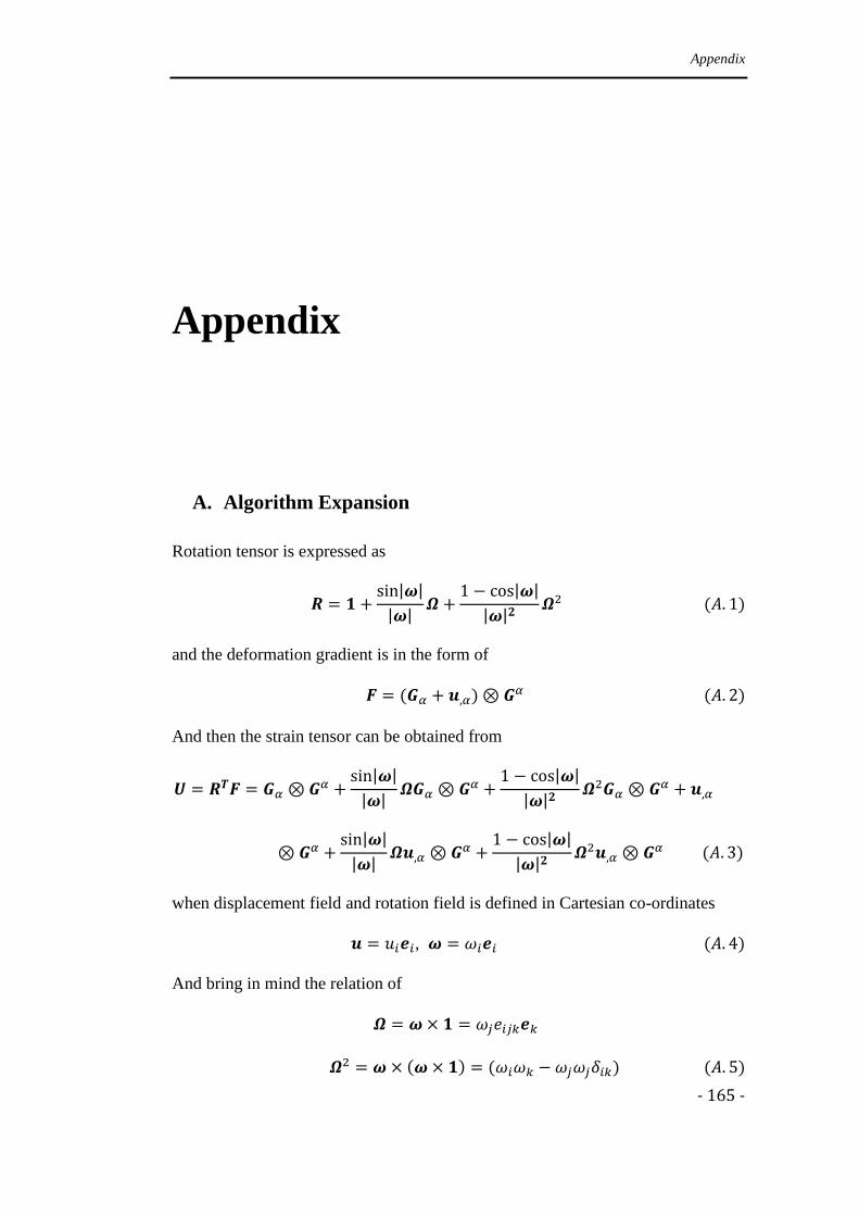
Appendix
- 165 -
Appendix
A. Algorithm Expansion
Rotation tensor is expressed as
and the deformation gradient is in the form of
And then the strain tensor can be obtained from
when displacement field and rotation field is defined in Cartesian co-ordinates
,
And bring in mind the relation of
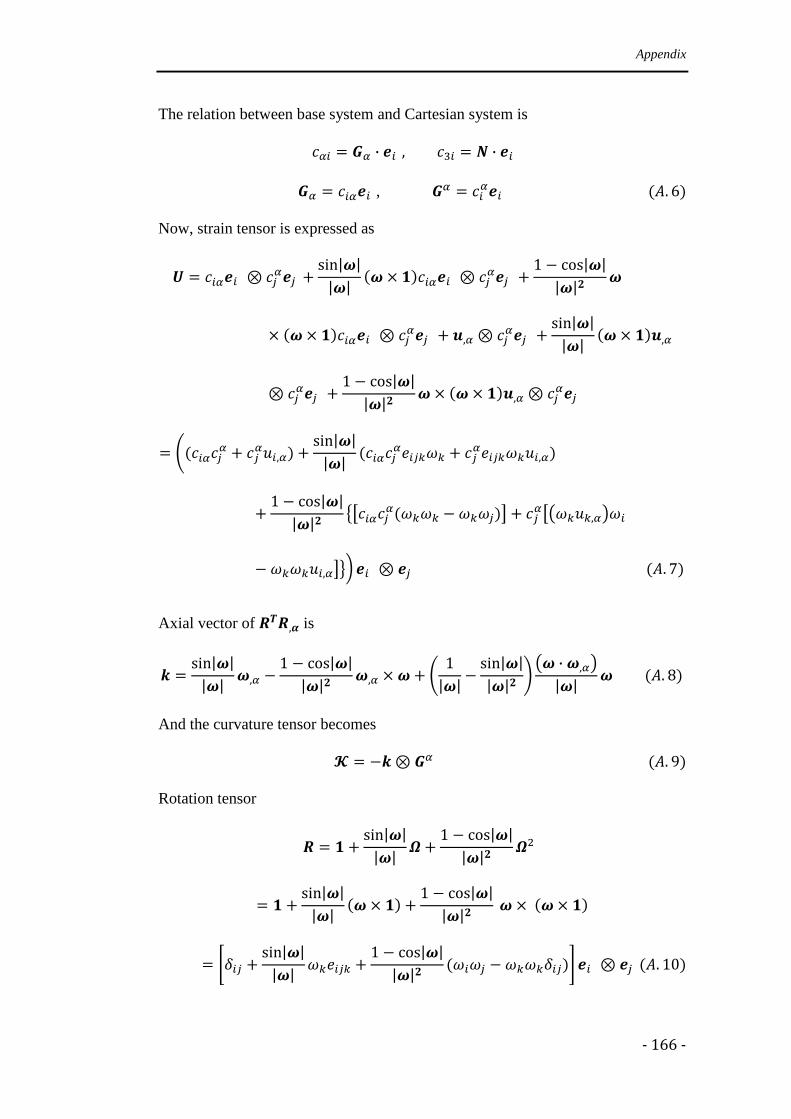
Appendix
- 166 -
The relation between base system and Cartesian system is
,
Now, strain tensor is expressed as
Axial vector of is
And the curvature tensor becomes
Rotation tensor
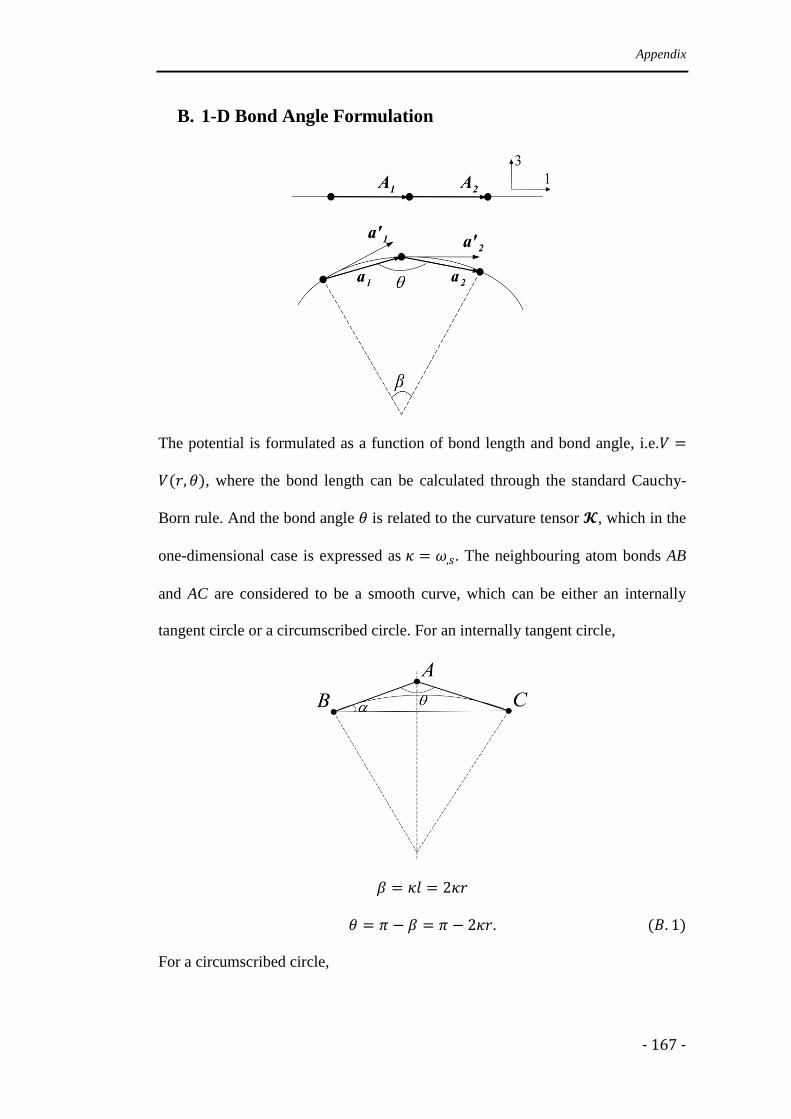
Appendix
- 167 -
B. 1-D Bond Angle Formulation
The potential is formulated as a function of bond length and bond angle, i.e.
, where the bond length can be calculated through the standard Cauchy-
Born rule. And the bond angle is related to the curvature tensor , which in the
one-dimensional case is expressed as . The neighbouring atom bonds AB
and AC are considered to be a smooth curve, which can be either an internally
tangent circle or a circumscribed circle. For an internally tangent circle,
For a circumscribed circle,
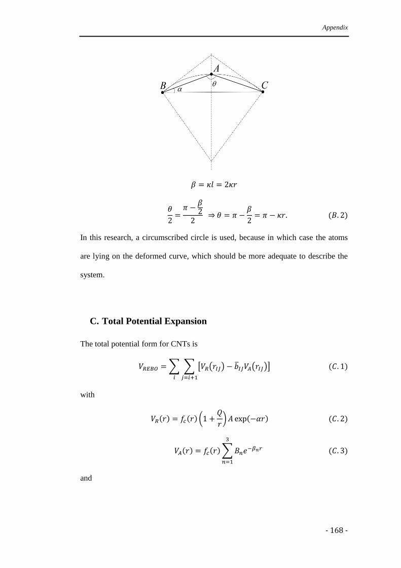
Appendix
- 168 -
In this research, a circumscribed circle is used, because in which case the atoms
are lying on the deformed curve, which should be more adequate to describe the
system.
C. Total Potential Expansion
The total potential form for CNTs is
with
and
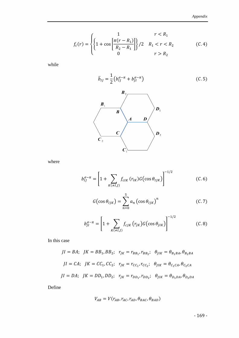
Appendix
- 169 -
while
where
In this case
Define
Appendix
- 170 -
Then the total potential is
The bond lengths are
where .
The deformed bond vectors are
And the bond angles are
where
corresponding to .
Define bond lengths , , , ,
, ,
, ,
as
(i=1,2,…,9) and bond angles , , , , , , ,
, as (i=1,2,…,9), inner displacement can be determined by
where strain energy density .
Force tensor can be obtained from
Appendix
- 171 -
Couple tensor can be expressed as
Stretch modulus-like tensor
where
And bending modulus-like tensor
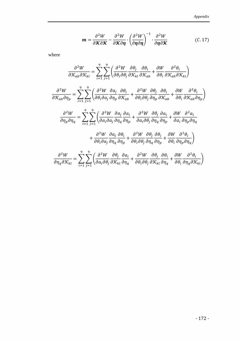
Appendix
- 172 -
where