University of California

Los Angeles

Singular Solutions and Pattern Formation inAggregation Equations

A dissertation submitted in partial satisfaction

of the requirements for the degree

Doctor of Philosophy in Mathematics

by

Hui Sun

2013

c� Copyright by

Hui Sun

2013

Abstract of the Dissertation

Singular Solutions and Pattern Formation inAggregation Equations

by

Hui Sun

Doctor of Philosophy in Mathematics

University of California, Los Angeles, 2013

Professor Andrea L. Bertozzi, Committee Chair, Chair

In this work, we study singular solutions and pattern formation in aggregation equations

and more general active scalar problems.

We derive a generalization of the Birkho↵-Rott equation to the case of active scalar prob-

lems with both gradient and divergence free structures. We present numerical simulations of

this model demonstrating how the gradient part and the divergence free part of K influence

each other and cause some nonlinear e↵ects. Examples include superfluids, classical fluids

and swarming models.

The rest of this thesis focuses on aggregation models with gradient flow structure. The

discrete version of the continuum aggregation equation is the kinematic equation xi

=

�mi

Pj 6=i

rU(|xi

� xj

|), 8 1 i N . For both discrete and continuum versions, we

use linear stability analysis of a ring equilibrium to classify the morphology of patterns

in two dimensions. Conditions are identified that assure the linear well-posedness of the

ring. In addition, weakly nonlinear theory and numerical simulations demonstrate how a

ring can bifurcate to more complex equilibria. Moreover, linear stability analysis of clusters

equilibrium patterns are also investigated in both two-dimensional and higher-dimensional

cases.

We then apply our stability results of ring patterns and clusters patterns to a family

ii

of exact collapsing similarity solutions to the aggregation equation with pairwise potential

U(r) = r�/�. It was previously observed that radially symmetric solutions are attracted to

a self-similar collapsing shell profile in infinite time for � > 2 in all dimensions. The stability

analysis for ring patterns and clusters patterns shows that the collapsing shell solution is

stable for 2 < � < 4, while always unstable and destabilizes into clusters that form a simplex

for � > 4. This holds in all spatial dimensions.

iii

The dissertation of Hui Sun is approved.

Je↵rey D. Eldredge

John B. Garnett

Russel E. Caflisch

Andrea L. Bertozzi, Committee Chair, Committee Chair

University of California, Los Angeles

2013

iv

To my family and friends

v

Table of Contents

1 Introduction . . . . . . . . . . . . . . . . . . . . . . . . . . . . . . . . . . . . . . 1

1.1 An Introduction to Aggregation Swarming Models . . . . . . . . . . . . . . . 1

1.2 Connections Between the Fluid Equations and Aggregation Problems . . . . 2

1.3 H-Stability and Singular Swarming Patterns . . . . . . . . . . . . . . . . . . 5

1.4 Finite Time Blowup and Self Similar Collapsing . . . . . . . . . . . . . . . . 8

1.4.1 Finite Time Blowup for the Discrete Case . . . . . . . . . . . . . . . 9

1.4.2 Finite Time Blowup for the Continuum Case . . . . . . . . . . . . . . 11

1.4.3 Self-Similar Collapsing . . . . . . . . . . . . . . . . . . . . . . . . . . 12

1.5 Outline for the Rest of the Thesis . . . . . . . . . . . . . . . . . . . . . . . . 12

2 Generalized Birkho↵-Rott Equation for 2D Active Scalar Equations . . 14

2.1 Derivation of the Generalized Birkho↵-Rott Equation . . . . . . . . . . . . . 14

2.2 Numerical Method . . . . . . . . . . . . . . . . . . . . . . . . . . . . . . . . 15

2.2.1 Algorithm . . . . . . . . . . . . . . . . . . . . . . . . . . . . . . . . . 16

2.2.2 Convergence Study . . . . . . . . . . . . . . . . . . . . . . . . . . . . 17

2.2.3 Verification of Method . . . . . . . . . . . . . . . . . . . . . . . . . . 18

2.3 Kernels of Mixed Type . . . . . . . . . . . . . . . . . . . . . . . . . . . . . . 25

2.3.1 Example 1: Superfluids . . . . . . . . . . . . . . . . . . . . . . . . . . 25

2.3.2 Biological Swarming . . . . . . . . . . . . . . . . . . . . . . . . . . . 35

3 Stability of Ring Patterns in R2 . . . . . . . . . . . . . . . . . . . . . . . . . 42

3.1 Discrete and Continuum Models . . . . . . . . . . . . . . . . . . . . . . . . . 42

3.2 Linear Stability of the Ring Solution in R2 . . . . . . . . . . . . . . . . . . . 43

vi

3.2.1 with Discrete Model . . . . . . . . . . . . . . . . . . . . . . . . . . . 43

3.2.2 with Continuum Model . . . . . . . . . . . . . . . . . . . . . . . . . . 45

3.2.3 Numerical Examples . . . . . . . . . . . . . . . . . . . . . . . . . . . 46

3.3 Linear Stability of the Shell Solution in Rd . . . . . . . . . . . . . . . . . . . 49

3.4 Weakly Nonlinear Analysis: Low Mode Bifurcations . . . . . . . . . . . . . . 51

3.4.1 Numerical Example . . . . . . . . . . . . . . . . . . . . . . . . . . . . 55

4 Stability of Cluster Patterns in Rd . . . . . . . . . . . . . . . . . . . . . . . . 57

4.1 Stability of Clusters in R2 . . . . . . . . . . . . . . . . . . . . . . . . . . . . 57

4.2 Stability of Clusters in General Space Dimensions . . . . . . . . . . . . . . . 60

5 Stability and Clustering of Self-Similar Solutions to Aggregation Equa-

tions . . . . . . . . . . . . . . . . . . . . . . . . . . . . . . . . . . . . . . . . . . . . 66

5.1 Similarity Transformation . . . . . . . . . . . . . . . . . . . . . . . . . . . . 67

5.2 Linear Stability of Shell Solutions . . . . . . . . . . . . . . . . . . . . . . . . 69

5.2.1 Linear Stability of Shell Solution in Rd . . . . . . . . . . . . . . . . . 69

5.2.2 Particle Simulations on Shell Stability . . . . . . . . . . . . . . . . . 70

5.3 Cluster Stability . . . . . . . . . . . . . . . . . . . . . . . . . . . . . . . . . . 75

5.3.1 Stability of Clusters in R2 . . . . . . . . . . . . . . . . . . . . . . . . 75

5.3.2 Numerical Simulations of Cluster Stability in R2 . . . . . . . . . . . . 75

5.3.3 Stability of Clusters in Rd . . . . . . . . . . . . . . . . . . . . . . . . 77

5.3.4 Numerical Simulations on Simplex Configuration . . . . . . . . . . . 77

5.4 Appendix of Chapter 5: Proof of Inequality (5.22) . . . . . . . . . . . . . . . 79

6 Conclusion and Future Works . . . . . . . . . . . . . . . . . . . . . . . . . . . 82

vii

References . . . . . . . . . . . . . . . . . . . . . . . . . . . . . . . . . . . . . . . . . 84

viii

List of Figures

1.1 Evolution of an irregular swarm patch under model (1.3), from top to bot-

tom, left to right, t = 0, 1, 2, 3, 7, 10. Reprent of C. M. Topaz and A. L.

Bertozzi, “ Swarming patterns in a two-dimensional kinematic model for bi-

ological groups” [TB], SIAM Journal on Applied Mathematics, Vol. 65, pp.

152-174, Copyright (2004) by SIAM. . . . . . . . . . . . . . . . . . . . . . . 3

1.2 H-stability diagram of Morse Potential. Reprent from M.R. D’Orsogna, Y.L.

Chuang, A.L. Bertozzi and L.S. Chayes, “Self-propelled particles with soft-

core interactions: patterns, stability and collapse” [DCBC], Physical Review

Letters, Vol. 96, 104302, Copyright (2006) by the American Physical Society. 6

1.3 Snapshots of swarms for di↵erent choices of C and l, resulting in di↵erent

kinds of patterns, including mill, clump, ring clump, and ring. Reprent from

M.R. D’Orsogna, Y.L. Chuang, A.L. Bertozzi and L.S. Chayes, “Self-propelled

particles with soft-core interactions: patterns, stability and collapse” [DCBC],

Physical Review Letters, Vol. 96, 104302, Copyright (2006) by the American

Physical Society. . . . . . . . . . . . . . . . . . . . . . . . . . . . . . . . . . 7

1.4 Phase Diagram for the first order model. Reprent from Y.-L. Chuang, Y. R.

Huang, M. R. D’Orsogna, and A. L. Bertozzi, “Multi-vehicle flocking: scalabil-

ity of cooperative control algorithms using pairwise potentials” [CHDB], IEEE

International Conference on Robotics and Automation, 2292-2299, c�2007

IEEE. . . . . . . . . . . . . . . . . . . . . . . . . . . . . . . . . . . . . . . . 8

2.1 The initial condition for the elliptically loaded example ( dashed line) and

the simulated fuselage flap configuration example (solid line). Figure (a) is a

plot of the initial circulation against ↵, and Figure (b) is a plot of the initial

density P against ↵. . . . . . . . . . . . . . . . . . . . . . . . . . . . . . . . 19

ix

2.2 The numerical solution at t = 0, 1, 2, 4 for the elliptically loaded wing example

using equations (2.8), (2.9) with (2.13). We take � = 0.05, �t=0.01, and we

use adaptive mesh refinement. . . . . . . . . . . . . . . . . . . . . . . . . . . 20

2.3 The numerical solution for the simulated fuselage flap configuration example

using equations (2.8) and (2.9). We take � = 0.1, �t=0.01, and we use

adaptive mesh refinement. . . . . . . . . . . . . . . . . . . . . . . . . . . . . 21

2.4 The numerical solution for the periodic perturbed ring example using equa-

tions (2.8), (2.9), with (2.13). We take � = 0.05, �t = 0.01, and we use

adaptive mesh refinement. . . . . . . . . . . . . . . . . . . . . . . . . . . . . 22

2.5 The comparison of the numerical solution of the radius of rings. In the above

6 pictures, a, c and e are the plot of the radius using equations (2.18) and

(2.19); b, d and f are the plot of the radius computed using equations (2.8)

and (2.9). a and b are the solutions for the one ring case; c and d are the

solutions for the two rings case; e and f are the solutions for the three rings

case. . . . . . . . . . . . . . . . . . . . . . . . . . . . . . . . . . . . . . . . . 23

2.6 Plot the evolution of the vortex density sheet at t = 1 for several values of

✓ with initial conditions (2.23). From outside to inside ✓ = �⇡/2, �5⇡/12,

�⇡/3, �⇡/4,�⇡/6, �⇡/12, and 0. The asterisks represent the point that was

initially positioned at (1, 0). . . . . . . . . . . . . . . . . . . . . . . . . . . . 26

2.7 Plot of the rotation angles at t = 1 with respect to parameter ✓. The solid

curve corresponds to the initial condition of a perturbed ring. The dashed

curve corresponds to an initial condition of an unperturbed ring. . . . . . . . 27

2.8 The solution at time t=1.5 for four di↵erent values of ✓. The asterisk indicates

the position of the point initialized at (1, 0). . . . . . . . . . . . . . . . . . . 28

2.9 Subsequent enlargements of a particular roll-up in picture (d) from Figure 2.8

using 12530 grid points. . . . . . . . . . . . . . . . . . . . . . . . . . . . . . 29

x

2.10 The solution to the periodic line problem at time t = 1, with initial condition

✏ sin(2⇡↵). (a). ✓ = �⇡/2, wind up number= 2.64; (b). ✓ = �5⇡/12, wind

up number= 5.04; (c). ✓ = �⇡/3, wind up number= 4.12; (d). ✓ = �⇡/4,wind up number= 1.60. . . . . . . . . . . . . . . . . . . . . . . . . . . . . . . 31

2.11 The solution to the linearized problem at time t = 1.3 with initial condition

✏1 sin(2⇡↵). The solid curve is for ✓ = �⇡/2; the dashed curve is for ✓ =

�5⇡/12; the dotted-dashed curve is for ✓ = �⇡/3. . . . . . . . . . . . . . . . 33

2.12 Time evolution of both the curve and density with ⌘(↵, 0) = 0.01 sin(2⇡↵)

with ✓ = �5⇡/12. This pure density perturbation leads to both a curvature

and density singularity formation. . . . . . . . . . . . . . . . . . . . . . . . . 34

2.13 The solution at time t=50 for �1 = 1 and varying values of �2. . . . . . . . . 36

2.14 The solution at time t=25 for �2 = 1 and varying values of �1. . . . . . . . . 37

2.15 By choosing parameters d and r, the spin direction of the outer arms are

di↵erent. . . . . . . . . . . . . . . . . . . . . . . . . . . . . . . . . . . . . . . 38

2.16 The initial condition as a circle, with the angular velocity it generates to a

point with distance ✏ on the right of the circle. . . . . . . . . . . . . . . . . 38

2.17 Integral I as a function of �. I(0.879)=0.000171 and I(0.878)=-0.003721,

indicating that the zero lies between 0.878 and 0.879. . . . . . . . . . . . . . 38

2.18 The solution at time t = 0, 3, 11, 15, with initial conditions (2.23) and (2.35)

with d = 1, r = 1, r = 0.2, �1 = 0.01, and �2 = 0.5 . . . . . . . . . . . . . . . 40

3.1 Simulation of (3.1) under interaction law (3.27) or (3.28) with certain param-

eter choices on a and b. . . . . . . . . . . . . . . . . . . . . . . . . . . . . . . 47

xi

3.2 Simulation of (3.1) under interaction law (3.27) or (3.28) with certain param-

eter choices. Simulation size: N = 400 individuals. First column, t = 0;

Second column, t = 2; Third column, t = 50; Forth column, t = 1000. First

row, tanh kernel (3.27), with a = 10, b = 0.1; Second row, power law kernel

(3.28), with a = 0.5, b = 6; Third row, power law kernel (3.28), with a = 0.5,

b = 4. . . . . . . . . . . . . . . . . . . . . . . . . . . . . . . . . . . . . . . . 48

3.3 The most positive eigenvalue of M(m) as defined in (3.26), for modes m

ranging from 1 to 20. Left: tanh kernel (3.27), with a = 10, b = 0.1; Middle:

power law kernel (3.28), with a = 0.5, b = 6; Right: power law kernel (3.28),

with a = 0.5, b = 4. . . . . . . . . . . . . . . . . . . . . . . . . . . . . . . . 49

3.4 Bifurcation diagram for interaction force (3.28), with p = 0.5. The solid curve

is calculated from Theorem 3.4.1. . . . . . . . . . . . . . . . . . . . . . . . . 55

4.1 regular tetrahedron on sphere . . . . . . . . . . . . . . . . . . . . . . . . . . 63

5.1 Simulations of (5.12) and (5.23) with various m and �. The ✏? on the first

row indicates that ✏k = 0 and ✏? = r0/100 for initial condition; the ✏k on the

second row indicates that ✏? = 0 and ✏k = r0/100 for initial condition. We

use N = 100 particles to perform the simulation and these structures have

varying radii from 0.35� 0.6. . . . . . . . . . . . . . . . . . . . . . . . . . . 72

5.2 Simulations for time evolution of (5.12) and (5.23) with N = 100 particles

for m = 5(first row) and m = 7( second row), and � = 40. The initial

perturbation is tangential with ✏k = r0/100. The ⇤’s are the centers of mass. 72

xii

5.3 The eigenvalues of matrix M(m) given by (5.16) and (5.17), with respect to

di↵erent modes m. This plot is for two space dimensions, but for general

space dimensions the behavior has the same qualitative features. The solid

curves are for m even; while the dashed curves are for m odd. (a) plots the

bigger eigenvalue of the two; (b) is an enlargement of a long and thin region

in (a); (c) plots the smaller eigenvalue of the two. . . . . . . . . . . . . . . . 73

5.4 We plot the behavior of c?

and ckin (5.25) for various values of m. The

dashed curves are for m even, while the solid ones are for m odd. (a) plots the

tangential eigenvalues ckin (5.25); (b) an enlargement along the the �-axis

of (a); (c) plots the normal eigenvalues c?in (5.25). In (c), all the curves

except m = 2 intersect at � = 4 with value c?= �1/3. The curve for m = 3

intersects 0 at � = 8/3, indicating that mode 3 normal perturbation changes

stability at � = 8/3. . . . . . . . . . . . . . . . . . . . . . . . . . . . . . . . 76

5.5 Numerical simulation of the m clusters problem, with m = 3, 4, 5, 6, and

� = 3, 5, 7, and 9, each hole starting with n = 20 particles with fixed-center

small random perturbation. (a) and (b) are the plot of the particles at time

⌧ = 50 and ⌧ = 10000 respectively. . . . . . . . . . . . . . . . . . . . . . . . 78

5.6 Numerical simulation of (5.12) and (5.13) with n = 150 random initial points

in Rd. Capital letters correspond to simulations done for � = 3 and lower case

letters correspond to � = 5. First Row: Figures (A1) and (a1) are the final

computed steady states in d = 3. Similarly for (B1), (b1) in d = 4 though

the plots are projected into R3 by taking the first three coordinates. (C1) and

(c1) are for d = 5 and are projections into R3 by also taking the first three

coordinates. Second Row: (A2), (a2), (B2), (b2), (C2), and (c2) are plots of

the corresponding probability distributions of the normalized inner product

of any two points in the final steady state. . . . . . . . . . . . . . . . . . . . 79

xiii

List of Tables

2.1 Convergence rate in time and space. . . . . . . . . . . . . . . . . . . . . . . 18

2.2 Ring collapsing time prediction . . . . . . . . . . . . . . . . . . . . . . . . . 25

2.3 Table of wind up numbers . . . . . . . . . . . . . . . . . . . . . . . . . . . . 30

2.4 Table of wind up numbers . . . . . . . . . . . . . . . . . . . . . . . . . . . . 37

5.1 Summary of the stability of Sd�1 with respect to the power � and mode m. . 71

5.2 Stability table for center of mass of clusters, corresponding to the second kind

of instability. It is stable if and only if the eigenvalues of A(l) defined by

(5.26) are all nonpositive. . . . . . . . . . . . . . . . . . . . . . . . . . . . . 77

5.3 Stability table for m clusters, combining both kinds of instabilities. It is stable

if and only if conditions 1 and 2 in Theorem 4.2.2 are satisfied. . . . . . . . 77

xiv

Acknowledgments

First and foremost, I would like to thank my advisor, Professor Andrea Bertozzi, for her

continuous guidance and generous support throughout my graduate studies at UCLA. She

has o↵ered me great help not only in academic research, but also in academic writing as well

as literature review. Besides, she has also encouraged me to attend many conferences and

meetings, which has greatly broaden my perspective. I feel very grateful to have her as my

Ph.D. advisor.

I am especially grateful to Professor David Uminsky at the University of San Francisco

and Professor Theodore Kolokolnikov at Dalhousie University, for their help and collabo-

ration on the research projects, and many detailed discussion, insightful suggestions, and

important contributions. Without them, this thesis would not exist. Professor Kolokolnikov

derived the linear stability analysis of the ring solutions in R2. I am also very thankful to

Dr. James VonBrecht at UCLA, who introduced me to the spherical packing problem, and

explained to me shell stability in a general dimension.

I would also like to thank many other professors for their help on various topics: Professor

Russel Caflisch and Dr. Mark Rosin on the stability analysis of the virtual cathode problem;

Professor Chris Anderson on Chebyshev grid discretization, implementation of multigrid al-

gorithms, MPI, subversion, etc.; Professor Joseph Teran on the Immersed Boundary Method,

implementation of linear elasticity in 2D and 3D, and finite element methods; Dr. Christoph

Brune on compressive sensing, optical flow estimation, and optimal control on flow estima-

tion.

I would also like to express my gratitude to the committee members for their time to

review my thesis.

In addition, I would like to thank the sta↵ in the Math department, especially Mrs.

Maggie Albert, Mrs. Martha Contreras, and Mrs. Babette Dalton, for their hearty help on

many detailed aspects of graduate life, and their everyday smiling faces.

Lastly, my special thanks go to Dr. Yanghong Huang, and Dr. Yao Yao, who have helped

xv

me in many practical ways.

xvi

Vita

1985 Born, Shaoxing, Zhejiang Province, China

2008 B.S. (Mathematics), Chinese University of Hong Kong

2010 M.A. (Mathematics), University of California, Los Angeles

Publications

T. Kolokolnikov, H. Sun, D. Uminsky, A. L. Bertozzi, Stability of Ring Patterns Arising

from Two- Dimensional Particle Interactions, Physical Review E., 84(1), 2011.

H. Sun, D. Uminsky, A. L. Bertozzi, A Generalized Birkho↵-Rott Equation for Two-

Dimensional Active Scalar Problems, SIAM J. on Applied Math., 72(1), 2012.

H. Sun, D. Uminsky, A. L. Bertozzi, Stability and Clustering of Self-Similar Solutions

of Aggregation Equations, J. Math. Phys., special issue: Incompressible Fluids, Turbulence

and Mixing, 53(11), 2012.

A. L. Bertozzi, J. Von Brecht, H. Sun, T. Kolokolnikov, D. Uminsky, Ring Patterns and

Their Bifurcations in the Model of Biological Swarms, Comm. Math. Sci., 2012, submit-

ted.

xvii

CHAPTER 1

Introduction

1.1 An Introduction to Aggregation Swarming Models

Aggregation swarming behavior is observed in nature, ranging from microscopic bacterial

colonies [DVM, VBDFFVM] to macroscopic fish schooling, locust swarming, animal flock-

ing [TT, MZDT, S4, EWG, R2, RB], as well as human crowd dynamics [HKM]. Typically

this kind of behavior exhibits certain kinds of patterns that can be modeled by pairwise

interaction laws, typically with long range attraction and short range repulsion. One rea-

sonable model for the aggregation swarming behavior is the second order kinetic model:

[DCBC, CDMBC]

dxi

dt= v

i

,

mi

dvi

dt= ↵v

i

� �|vi

|2vi

�X

j 6=i

rU(|xi

� xj

|), (1.1)

where each individual is labeled i, with position xi

, velocity vi

, and mass mi

. The terms

↵vi

and �|vi

|2vi

are the self-propulsion and drag, respectively, yielding to an equilibrium

velocityp↵/�. The pairwise potential U is a function on the positive real axis, having a

local minimum at some rc

> 0, with U 0(r) < 0 for r < rc

and U 0(r) > 0 for r > rc

thus

having long range attraction and short range repulsion. Another simplified model is the first

order kinematic model: [KSUB, VUKB, VU, KHP]

dxi

dt= �m

i

X

j 6=i

rU(|xi

� xj

|). (1.2)

This is a reduced model compared to the kinetic model (1.1), in the sense that only the

change of position instead of the change of velocity is considered. This simplified model

1

(1.2) is closely connected to the active scalar equation [C, TB, BCL]

@⇢

@t+r · (⇢v) = 0, v = r?N ⇤ ⇢+rG ⇤ ⇢, (1.3)

where ⇢ is the active scalar, typically the density of an underlying material. Using the Hodge

decomposition, the velocity field v is composed of a divergence free part r?N and a gradient

part rG. The active scalar equation (1.3) arises in problems of vortex dynamics [MB, Y],

quasi-geostrophic flow [CMT] and superfluids [DP]. Equation (1.3) is a continuum limit of

(1.2) when the number of particles approaches infinity. The case where we have both r?N

and rG nonzero for the active scalar equation (1.3) is also studied for aggregation swarming

patterns in [TB]. Adding di↵usion to (1.3), we get the Keller-Segel equation: [KS]

@⇢

@t+r · (⇢rc) = �⇢, ��c = ⇢, (1.4)

where ⇢ is the density of bacteria, and c is the density of the chemo-attractant. Here the

kernel G would be the Newtonian potential.

1.2 Connections Between the Fluid Equations and Aggregation

Problems

One of the interesting swarm patterns observed in nature is the two-dimensional vortex-like

ant mill [S4]. It is a spiral shape with shape edges and nearly uniform density, exhibiting

certain similarity to the vortex patches in fluid dynamics. In [TB], Topaz and Bertozzi has

proved that in one dimension, uniform density traveling band solutions satisfying (1.3) never

exist, unless the kernel N or G is periodic, which is not biologically meaningful because the

sensitivity of an individual usually decays with distance.

In the same paper, in two dimensional case, the spiral vortex solutions to (1.3) are con-

structed and verified numerically (see Figure 1.1). The authors consider the incompressible

kernel, i.e., with G = 0. The reason for that choice is that biological swarms are able to

move and evolve in shape while maintaining their constant density. Then they choose the

2

Figure 1.1: Evolution of an irregular swarm patch under model (1.3), from top to bottom,

left to right, t = 0, 1, 2, 3, 7, 10. Reprent of C. M. Topaz and A. L. Bertozzi, “ Swarming

patterns in a two-dimensional kinematic model for biological groups” [TB], SIAM Journal

on Applied Mathematics, Vol. 65, pp. 152-174, Copyright (2004) by SIAM.

kernel N to be Gaussian with width d

N(r) =1

d2e�

r2

d2 , (1.5)

so that by setting d ! 0, (1.3) may be written as

@⇢

@t+ ⇡r · (⇢r?⇢) = 0, (1.6)

whose density profile does not change because the motion is perpendicular to the density

gradient. By setting d ! 1, r?N = 0, (1.3) becomes ⇢t

= 0 again. The authors then

consider a solution of constant density over a compact supported domain, a swarming patch,

3

and apply Green’s formula to formulate the velocity at the boundary of the swarming patch

v(x) = ⇢0

Z

@⌦

N(|x� y|)t(y)ds(y), (1.7)

where ⇢0 is the constant density of the swarming patch, ⌦ is the domain of the patch, and

t(y) is the unit tangential vector at point y. Taking ↵ 2 [0, 2⇡] as a Lagrangian parameter

for the boundary @⌦, (1.7) can be written as

x(↵, t)

@t= ⇢0

Z

0

2⇡N(|x(↵, t)� x(↵0, t)|)x↵

(↵0, t)d↵0, (1.8)

where by setting N(r) = log(r), it represents the vortex patch equation in the incompressible

inviscid fluids. Numerical simulation of (1.3) withG = 0, N given by (1.5), and initial density

uniform over an irregular domain results in swarming patches that are observed in bacteria,

fish, ants, etc. [BCCVG, OMB, PE, RNSL, S4]

The simulations illustrate the similarity between vortex patches in incompressible inviscid

fluids and swarm patches, which both exhibit rotational motion with long filaments. This

motivates our study for swarming sheets, which is analogous to vortex sheets. A vortex

sheet is a co-dimensional one sheet in surrounding fluid, where the velocity is discontinuous.

Unlike vortex patch, where vorticity is bounded pointwisely, a vortex sheet has vorticity

concentrated as a measure. Whereas the swarming sheet has individuals collapsing on a co-

dimensional one sheet, resulting a singular density concentrated as a measure. The swarming

sheet is studied in detail in chapter 2.

The formation of the singular swarming patterns, for example, solutions concentrated

on curves and clusters, although not observed in biological swarms, still have an applica-

tion in artificial swarms. This kind of phenomenon has introduced the topic of stability

prediction with respect to size. If a well-defined spacing among individuals persists, usually

swarming size increases with particle number, in a crystallization way. However, sometimes,

the size collapses as the number of individuals increases. In [DCBC, CDMBC], the authors

apply fundamental principles from thermodynamics, H-stability, to prediction the stability

of swarms, in regards to the possible collapse as the number of individuals increases.

4

1.3 H-Stability and Singular Swarming Patterns

In [DCBC, CDMBC], the authors use the H-stability criterion to analyze the first order

model (1.1),

dxi

dt= v

i

,

mi

dvi

dt= ↵v

i

� �|vi

|2vi

�X

j 6=i

rU(|xi

� xj

|),

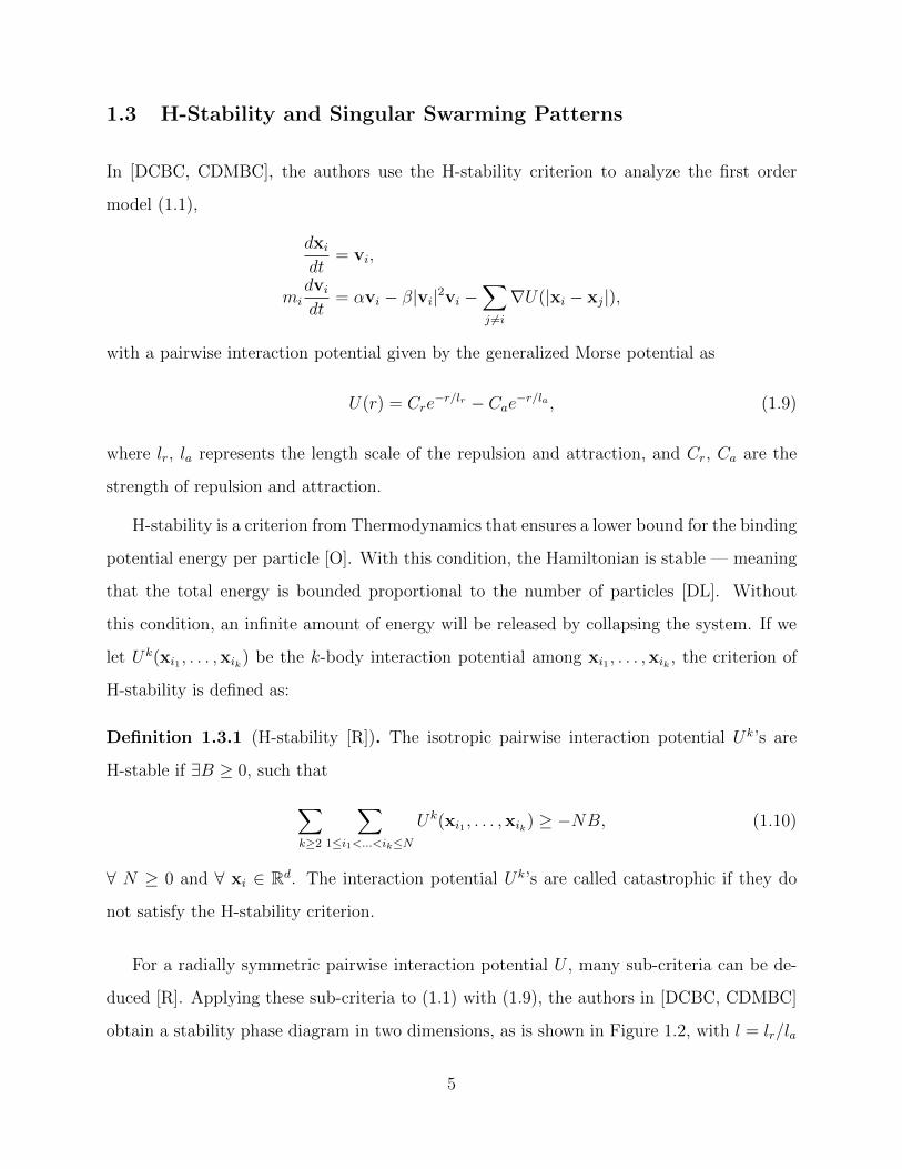
with a pairwise interaction potential given by the generalized Morse potential as

U(r) = Cr

e�r/lr � Ca

e�r/la , (1.9)

where lr

, la

represents the length scale of the repulsion and attraction, and Cr

, Ca

are the

strength of repulsion and attraction.

H-stability is a criterion from Thermodynamics that ensures a lower bound for the binding

potential energy per particle [O]. With this condition, the Hamiltonian is stable –– meaning

that the total energy is bounded proportional to the number of particles [DL]. Without

this condition, an infinite amount of energy will be released by collapsing the system. If we

let Uk(xi1 , . . . ,xik

) be the k-body interaction potential among xi1 , . . . ,xik

, the criterion of

H-stability is defined as:

Definition 1.3.1 (H-stability [R]). The isotropic pairwise interaction potential Uk’s are

H-stable if 9B � 0, such that

X

k�2

X

1i1<...<ikN

Uk(xi1 , . . . ,xik

) � �NB, (1.10)

8 N � 0 and 8 xi

2 Rd. The interaction potential Uk’s are called catastrophic if they do

not satisfy the H-stability criterion.

For a radially symmetric pairwise interaction potential U , many sub-criteria can be de-

duced [R]. Applying these sub-criteria to (1.1) with (1.9), the authors in [DCBC, CDMBC]

obtain a stability phase diagram in two dimensions, as is shown in Figure 1.2, with l = lr

/la

5

Figure 1.2: H-stability diagram of Morse Potential. Reprent from M.R. D’Orsogna, Y.L.

Chuang, A.L. Bertozzi and L.S. Chayes, “Self-propelled particles with soft-core interactions:

patterns, stability and collapse” [DCBC], Physical Review Letters, Vol. 96, 104302, Copy-

right (2006) by the American Physical Society.

and C = Cr

/Ca

. This diagram is obtained analytically, by examining the potential (1.9)

with the sub-criteria for H-stability as deduced in [R]. For details of the derivation of the

region that is H-stable or catastrophic, one may refer to [C2].

Figure 1.2 is divided into three main regions. Region V is repulsion dominant, and each

individual tends to escape from everyone else. Regions I, II, III, and IV are attraction

dominant regions, and are all catastrophic. Regions VI, VII are biologically relevant regions.

Among these regions, only regions V and VI are H-stable, with swarm patterns such as

coherent flocking or rigid-body rotation. However, in the remaining catastrophic regions,

interesting swarming patterns are observed, such as mill, clump, ring clump, ring, as plotted

6

in Figure 1.3. Whereas coherent flocking and milling are the most commonly observed animal

swarming patterns [PE, PVG, S4].

Figure 1.3: Snapshots of swarms for di↵erent choices of C and l, resulting in di↵erent kinds

of patterns, including mill, clump, ring clump, and ring. Reprent from M.R. D’Orsogna,

Y.L. Chuang, A.L. Bertozzi and L.S. Chayes, “Self-propelled particles with soft-core inter-

actions: patterns, stability and collapse” [DCBC], Physical Review Letters, Vol. 96, 104302,

Copyright (2006) by the American Physical Society.

In [CHDB], a simular stability analysis is carried out for the second order model (1.2),

with the same Morse potential (1.9). It is done through defining a Lyapunov function

and applying a weak maximum principle. The swarming patterns are classified into three

regimes: a collapsing state with all particles converging to the same point, a dispersive

state with particles dispersed into infinity, and a cohesive state with particles maintain fixed

relative distances. (see Figure 1.4).

Although H-stability predicts the scaling behavior of equilibrium configuration, never-

theless, the theory for symmetry breaking of the equilibrium configuration has not been in-

7

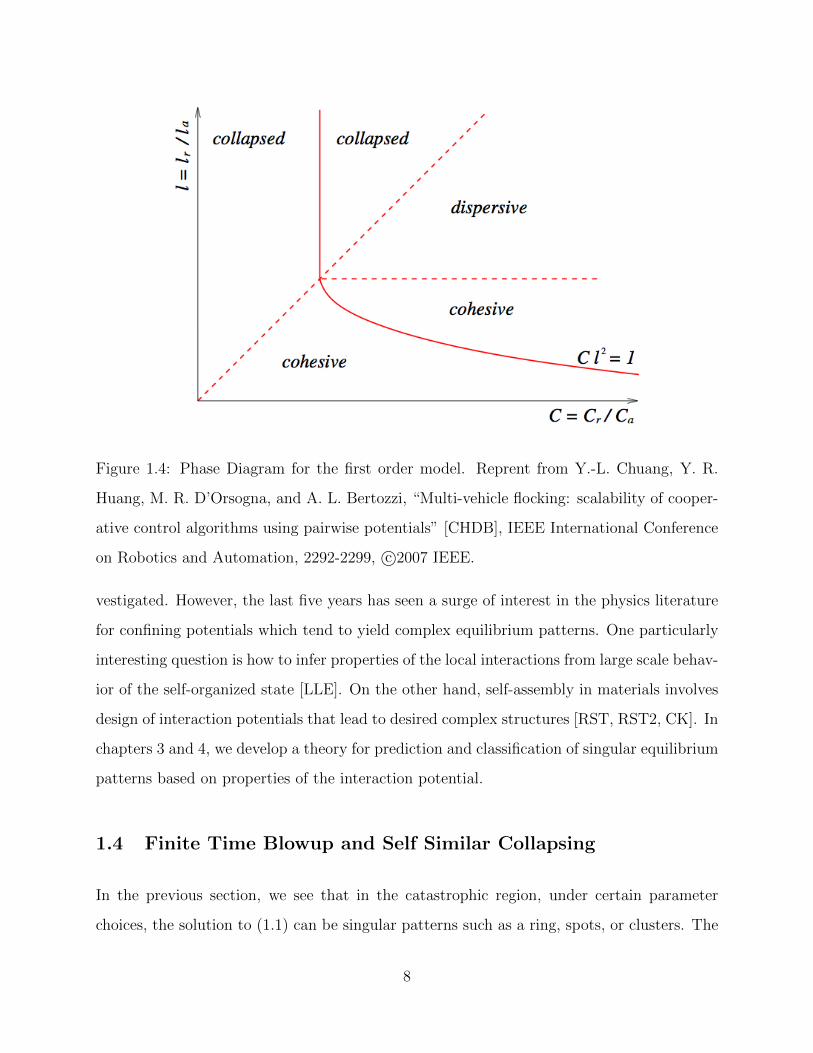
Figure 1.4: Phase Diagram for the first order model. Reprent from Y.-L. Chuang, Y. R.

Huang, M. R. D’Orsogna, and A. L. Bertozzi, “Multi-vehicle flocking: scalability of cooper-

ative control algorithms using pairwise potentials” [CHDB], IEEE International Conference

on Robotics and Automation, 2292-2299, c�2007 IEEE.

vestigated. However, the last five years has seen a surge of interest in the physics literature

for confining potentials which tend to yield complex equilibrium patterns. One particularly

interesting question is how to infer properties of the local interactions from large scale behav-

ior of the self-organized state [LLE]. On the other hand, self-assembly in materials involves

design of interaction potentials that lead to desired complex structures [RST, RST2, CK]. In

chapters 3 and 4, we develop a theory for prediction and classification of singular equilibrium

patterns based on properties of the interaction potential.

1.4 Finite Time Blowup and Self Similar Collapsing

In the previous section, we see that in the catastrophic region, under certain parameter

choices, the solution to (1.1) can be singular patterns such as a ring, spots, or clusters. The

8

formation of these kinds of singular patterns is related to blowup properties for aggregation

equations.

Recently, the finite time blow up problem of (1.3) with purely potential flow, i.e. N = 0,

has drawn much attention. The existence and uniqueness of solutions for rough initial data

and singular potential G has been proven for both one dimension [BV, BD] and n space

dimensions [L2]. Finite-time blow-up of solutions under rotationally symmetric kernels with

a Lipschitz point at the origin is also known [BL, BB]. For weak measure solutions the well-

posedness theory, uniqueness, and global existence has been recently explored [CDFLS, VB].

Furthermore, an Osgood condition on the kernel which is a necessary and su�cient condition

for infinite time blow up has also been derived [BL2, BCL].

The Osgood condition

Z 1

0

1

G0(r)dr = 1, (1.11)

is a necessary and su�cient condition for global existence of a bounded solution. If it is not

satisfied, i.e.

Z 1

0

1

G0(r)dr < 1, (1.12)

the solution blows up in finite time. Moreover, the bound on blowup time depends only on

the radius of the support of the initial data and the total mass of the solution.

The details of the blowup theorem with Osgood condition is described in the subsections

1.4.1 and 1.4.2.

1.4.1 Finite Time Blowup for the Discrete Case

In this case, one consider a particle system xi

2 Rd, with 1 i N , described by the

kinematic model (1.2). Assuming the center of mass at 0, and define

R(t) := max1jn

|xj

| = |xi

|, (1.13)

9

where xi

is the furthest particle from the center of mass. Then we have

d

dtR(t)2 = 2x

i

· dxi

dt= �2

X

j 6=i

mj

(xi

� xj

) · xi

|xi

� xj

| U 0(|xi

� xj

|). (1.14)

Since xi

is the furthest particle from the center of mass, we have (xi

� xj

) · xi

> 0, and

|(xi

� xj

)| < 2R. With the assumption that

U 0(r)

ris non-increasing for r > 0, (1.15)

we have

d

dtR(t)2 �U 0(2R(t))

R(t)

X

j 6=i

mj

(xi

� xj

) · xi

. (1.16)

Since the center of mass is at 0, we haveP

j 6=i

mj

(xi

� xj

) · xi

= MR(t)2, and hence

d

dtR(t) �M

2U 0(2R(t)). (1.17)

Since d

dt

R(t) 0 and U 0(2R(t)) � 0, with initial condition R(t = 0) = R0, we have

2

M

ZR0

0

1

U 0(2R)dR � �

ZR0

0

dt

dRdR = T ⇤, (1.18)

where T ⇤ is the blowup time. Thus, when the Osgood condition is not satisfied, we have

finite time blowup for the discrete system (1.2). The complete argument for the discrete

case is stated rigorously in the following theorem:

Theorem 1.4.1 (Collapse of the ODEs [BCL]). Consider the ODE system (1.2) satisfying

U(r)/r monotone decreasing, with U(r) defined and non-negative on (0,1). If U satisfies

the Osgood condition (1.11) then there exists a unique global-in-time forward solution with

no collisions, in which the particles converge to their center of mass in infinite time. If U

satisfies the non-Osgood condition (1.12) then there exists a unique global-in-time forward

solution with collisions, in which the particles eventually all merge at their center of mass

after finite time. In the latter case, for a given potential, an upper bound on the merger time

is a function of the radius of support of the initial data and the total mass only.

10

1.4.2 Finite Time Blowup for the Continuum Case

For the continuum case, the density is governed by (1.3)

@⇢

@t+r · (⇢v) = 0, v = r?N ⇤ ⇢+rG ⇤ ⇢,

in Rd, with N = 0. Then computing the divergence, we have

@⇢

@t+ v ·r⇢ = �⇢ div(rG ⇤ ⇢), (1.19)

which tells us that along characteristics, ⇢ is amplified by �G ⇤ ⇢. For special kind of kernel

G 2 C2, we have that

d

dtk⇢k

L

1 k�G ⇤ ⇢kL

1k⇢kL

1 (1.20)

k�GkL

1k⇢kL

1k⇢kL

1 . (1.21)

This provides an upper bound for the k⇢L

1k through Gronwall’s lemma. For potentials

satisfying Osgood condition (1.11), Bertozzi et. al. obtain the global in time L1 theorem.

Theorem 1.4.2 (Global-in time L1 and infinite time blowup for Osgood potentials [BCL]).

Consider (1.3) with the potentials N = 0 and G radially symmetric. Assume G00(r) > 0 and

that G(r)/r monotone decreasing in r. Then on the interval of existence (0, T ⇤)

d

dtk⇢k�1/d

L

1 � �C(d,M)G0(M1/dk⇢k�1/dL

1 ) (1.22)

holds. As a consequence, if G satisfies the Osgood condition (1.11) then for any compactly

supported non-negative L1 solution of the aggregation equation stays bounded for all time

and converges as t ! 1 to a Dirac mass of size M located at its center of mass cM

.

Furthermore, for potentials satisfying non-Osgood condition (1.12), Bertozzi et. al. [BCL]

derive a theorem for radially symmetric solutions.

Theorem 1.4.3 (Blow-up: radial case [BCL]). Consider equation (1.3) where the potential

N = 0 and G radially symmetric. Assume that G0(r) � 0 with G0(r) > 0 for r > 0,

11

and 9� > 0, such that G0 is monotone on [0, �). Also assume that G satisfies non-Osgood

condition (1.12). Suppose the initial data are radially symmetric, compactly supported and

bounded. Then there exists a finite time T ⇤ such that the unique weak solution ⇢(x, t) of

(1.3) satisfies

limt!T

⇤sup0⌧<t

k⇢(., ⌧)kL

q = +1 (1.23)

for all q � 2 (q > 2 for d = 2).

1.4.3 Self-Similar Collapsing

The above theorems provide a necessary and su�cient condition for finite time blowup of

solutions to kinematic model or aggregation equation,under certain conditions. Huang and

Bertozzi [HB, HB2] study the blowup behavior of (1.3) with power law kernels G(r) = r�/�.

The Osgood condition guarantees finite time blow-up for � < 2, and infinite time blow-up

for � > 2. Furthermore, it is well understood that the symmetric collapsing solutions exhibit

self similarity under this power law kernel. In chapters 4 and 5 we study the symmetry

breaking of such solutions.

1.5 Outline for the Rest of the Thesis

We explore the relation between fluids and active scalar equations in Chapter Two, with a

focus on sheet like solutions, in which the density ⇢ is concentrated on a codimension-one

surface. These are a generalization of vortex sheets to flows with both divergence free and

gradient components. In Chapter Three, we study the linear stability of ring solutions for

both the continuum model and discrete model in R2, as well as weakly nonlinear bifurcation

theory. In Chapter Four, we study the singular patterns that are formed with clusters, in

a general dimension. Furthermore, in Chapter Five, we apply our stability theory of the

singular patterns composed of shells and dots to a family of self-similar collapsing shell

solutions to the aggregation equation with power law kernel. We conclude and discuss

12

possible future research.

13

CHAPTER 2

Generalized Birkho↵-Rott Equation for 2D Active

Scalar Equations

If the kernel K of the active scalar equations

@⇢

@t+r · (⇢v) = 0, ⇢(x, 0) = ⇢0(x), (2.1)

v = K ⇤ ⇢ = r?N ⇤ ⇢+rG ⇤ ⇢, (2.2)

takes only the divergence free part r?N , whereas N(r) = ln |r|, equations (2.1) and (2.2)

becomes the vorticity equation for 2D inviscid incompressible fluids, with the active scalar

⇢ being the vorticity. The vorticity equation further reduces to Birkho↵-Rott equation

@X

@t=

1

2⇡P.V.

Z

S

(X(�, t)�X(�0, t))?

|X(�, t)�X(�0, t)|2 d�0, (2.3)

for those solutions with initial vorticity ⇢0 living on a curve, where the vortex sheet S has a

Lagrangian representation X(�, t), and circulation � is the integral of the vorticity ⇢ along

the sheet.

In this chapter, we generalize the Birkho↵-Rott equation for describing the 2D active

scalar equation when the solution is supported on 1D curve(s).

2.1 Derivation of the Generalized Birkho↵-Rott Equation

For solutions of (2.1) and (2.2) living on an 1D sheet S with a Lagrangian representation

X(↵) with ↵ 2 D, the active scalar ⇢ takes the form

⇢(x, t) =

Z

DP (↵, t)�(x�X(↵, t))|X

↵

|d↵, (2.4)

14

where the subscript ↵means derivative, and hence equation (2.1) is defined in a distributional

sense, that is, 8 2 C10 (R2, [0,1)),

Z 1

0

Z

D(

t

(X(↵, t), t) + v ·r (X(↵, t), t))P (↵, t)|X↵

|d↵dt = 0, (2.5)

with v = Xt

(↵, t) being the velocity at which the sheet evolves. Applying integration by

parts to (2.5), we arrive atZ 1

0

Z

D (X(↵, t), t) (P (↵, t)|X

↵

|)t

d↵dt = 0. (2.6)

Since (2.6) holds for any 2 C10 (R2, [0,1)), we must have

(P (↵, t)|X↵

|)t

= 0. (2.7)

A further simplification of (2.7) coupled with (2.2) gives us the generalized Birkho↵-Rott

equation

@P (↵, t)

@t+ P (↵, t)

X↵

· v↵

X↵

·X↵

= 0, (2.8)

@X(↵, t)

@t= v = K ⇤ P = r?N ⇤ P +rG ⇤ P. (2.9)

Notice that (2.7) is really conservation of mass (2.1) restricted on a curve, while it is a

generalization of Birkho↵-Rott equation in describing evolution of a sheet with a general

kernel K that is of mixed type, i.e., with both divergence free part r?N and gradient part

rG. The interactions between these two parts of K exhibit interesting nonlinear dynamics,

as we describe later in this chapter.

2.2 Numerical Method

We implement equations (2.8) and (2.9) using a fourth order Runge Kutta method in time

and centered di↵erence discretization in space. In addition, we apply an adaptive mesh

method using cubic interpolation for several of the more complicated examples in sections

2.2.3.1 where more resolution is required. We briefly present this algorithm below.

15

2.2.1 Algorithm

Throughout the section, we use N to denote the number of space discretization and M to

denote the total number of time steps. Since the spatial mesh is adaptive, N may vary from

step to step. Superscripts represent time steps, while subscripts are for spatial nodes. For

example, we use ↵n

i

to identify the value of Lagrangian parameter at the ith discretization

node, nth time step. We adopt the notations Xn, vn and Pn for vectors with entries

Xn

i

= X(↵i

, tn), vn

i

= v(↵i

, tn), and P n

i

= P (↵i

, tn),

respectively, and F1 and F2 be another two vectors with elements

F1,i(P,X,v) =@P n

j

@t= �P n

j

(Xj+1 �X

j�1) · (vj+1 � vj�1)

(Xj+1 �X

j�1) · (Xj+1 �Xj�1)

, (2.10)

F2,i(P,v) = vn

i

=X

j

K(Xn

i

�Xn

j

)P n

j

|�Xj

| =X

j

K(Xn

i

�Xn

j

)P n

j

|Xj+1 �X

j�1||↵

j+1 � ↵j�1| . (2.11)

respectively. Then the 4th order Runge Kutta algorithm is applied to (2.8) and (2.9):

1. ⇢n

1 = F2(Pn,Xn,Vn

1 ), Vn

1 = F1(Pn,Xn);

2. ⇢n

2 = F2(Pn +�t⇢n

1/2,Xn +�tVn

1/2,Vn

2 ), Vn

2 = F1(Pn +�t⇢n

1/2,Xn +�tVn

1/2);

3. ⇢n

3 = F2(Pn +�t⇢n

2/2,Xn +�tVn

2/2,Vn

3 ), Vn

3 = F1(Pn +�t⇢n

2/2,Xn +�tVn

2/2);

4. ⇢n

4 = F2(Pn +�t⇢n

3 ,Xn +�tVn

3 ,Vn

4 ), Vn

4 = F1(Pn +�t⇢n

3 ,Xn +�tVn

3 );

5. Pn+1 = Pn+�t(⇢n

1 +2⇢n

2 +2⇢n

3 +⇢n

4 )/6, Xn+1 = Xn+�t(Vn

1 +2Vn

2 +2Vn

3 +Vn

4 )/6.

After each Runge Kutta step, we update the tolerance in our adaptive mesh by first setting

✏ = min(total length of curve/N, ✏). We then consider the distance between consecutive

points |Xi+1 �X

i

|. If it is greater than ✏, we add one node ↵i+1/2 = (↵

i

+ ↵i+1)/2 between

them, with values of P (↵i+1/2) and X(↵

i+1/2) evaluated using cubic interpolation. We then

reorder the ↵i

’s to discard the half indices, so that i 2 N and ↵i

is monotone in i.

16

2.2.2 Convergence Study

To verify the convergence of our method, we use the periodic perturbation example in section

2.2.3.1 below. Since the exact solution to this example is unknown, we derive the order

of convergence by computing successive di↵erences between numerical solutions. We then

double the number of points (in time or in space respectively) and then apply equation (2.12)

to estimate the convergence rate.

For the convergence in time, let (X1,P1), (X2,P2), (X3,P3) and (X4,P4) be used to

denote the numerical solution for time discretization M = 10, 20, 40, 80 respectively, at

T = 0.1, with space discretization N = 100. Then the approximate convergence rate can be

calculated as follows

Conv. rate ⇡ log(||ei

||2/||ei+1||2)/ log 2, (2.12)

where ei

can be taken as vectors Xi

�Xi+1 or Pi

�Pi+1. Notice that subscripts i, i+1 refer

to consecutive refinements in either space or time.

For the convergence in space, we use the same notations with lower case letters (x1,p1),

(x2,p2), (x3,p3

) and (x4,p4) to denote the solution for space discretization N = 100, 200,

400, 800 respectively, at time T = 0.1, with M = 100. We use formula (2.12) to compute

the approximate convergence rate as before, except that ei

is taken to be vectors xi

�xi+1 or

pi

� pi+1

. We also compute the convergence in space with the e↵ect of cubic interpolation

by starting with the same parameter setting, and successively halving the adaptive tolerance

✏. We obtain solutions (z1,p1), (z2,p2

), (z3,p3) and (z4,p4

), and then use formula (2.12) to

compute the approximate convergence rate. From table (2.1), we can see that the convergence

is approximately 4th order in time, and 2nd order in space (as expected). We also see that

the convergence for cubic interpolation adaptive method is approximately 2nd order.

From the onset we designed a numerical scheme for this general curve evolution prob-

lem which is 4th order in time and 2nd order in space. For comparison to the simulation

of the classical vortex sheet problem many numerical schemes have been developed which

have varying convergence orders [CL, K, K2, L, P], including spectrally accurate convergent

17

Table 2.1: Convergence rate in time and space.

Convergence in time

M ||Xi

�Xi+1||2 conv. rate ||P

i

�Pi+1||2 conv. rate

10

20 6.1748e-07 7.7979e-06

40 4.6074e-08 3.7444 5.7844e-07 3.7528

80 3.1409e-09 3.8747 3.9661e-08 3.8664

Convergence in space

N ||xi

� xi+1||2 conv. rate ||p

i

� pi+1

||2 conv. rate

100

200 3.6915e-05 1.2083e-03

400 4.7733e-06 2.9511 2.7878e-04 2.1158

800 1.1654e-06 2.0342 6.9860e-05 1.9966

Convergence rate for cubic interpolation

✏ ||xi

� xi+1||2 conv. rate ||p

i

� pi+1

||2 conv. rate

0.06

0.03 4.7311e-06 2.7239e-04

0.015 1.1345e-06 2.0601 6.5691e-05 2.0519

0.0075 2.8138e-07 2.0115 1.6136e-05 2.0255

schemes [S, HLK].

2.2.3 Verification of Method

Here we test the new algorithm on well known examples. First, in section 2.2.3.1 we recom-

pute well studied solutions of vortex sheets in the literature using the new code and show

that the resulting solution are in excellent agreement to previously published results. Second,

in section 2.2.3.2 we compute concentric collapsing ring solutions in the purely aggregating

case and verify good agreement as compared to the known special solutions of the associated

18

ODE theory.

2.2.3.1 Case 1: Incompressible Vortex Sheet Examples

In this section we verify our model by implementing our method to simulate three vortex

sheet problems for the 2D Euler equations. This corresponds to setting N = 12⇡ log |r| and

G = 0 in equations (2.1) - (2.2). As mentioned previously, the motion of the vortex sheet is

governed by the Birkho↵-Rott equation (2.7) and it is well known that (2.7) is ill-posed due

to the Kelvin-Helmholtz instability, see [MB, SSBF]. Thus, in order to implement our model

to simulate equations (2.1) - (2.2) we must desingularize the kernel. Several approaches have

been developed to compute the evolution of vortex sheets [AG] which address the Kelvin-

Helmholtz instability. For our method we use Krasny’s [K] direct desingularization of the

kernel N ,

r?N�

=(X(�, t)�X(�0, t))?

|X(�, t)�X(�0, t)|2 + �2, (2.13)

where � is a regularization parameter, to compute the examples in this section.

Our first verification simulates the classical elliptically loaded wing example, [K2]. The

initial Lagrangian parameterization for the elliptically loaded wing is X(↵) = (x, y) = (2↵�1, 0), where ↵ 2 [0, 1]. The initial distribution of vorticity P is set by P = �d�/dx, where

� =p1� x2 is the circulation of the vortex sheet, as depicted in Figure 2.1.

−1 −0.5 0 0.5 10

0.5

1

1.5

2

−1 −0.5 0 0.5 1−10

−5

0

5

10(a) (b)

Figure 2.1: The initial condition for the elliptically loaded example ( dashed line) and the

simulated fuselage flap configuration example (solid line). Figure (a) is a plot of the initial

circulation against ↵, and Figure (b) is a plot of the initial density P against ↵.

19

Using our adaptive point method with error tolerance ✏ = 0.075, we initialize the sheet

using 401 points and at T = 4 the final number of points is 3171. The results are plotted in

Figure 2.2 and the observed roll-up is in excellent agreement with Figure 2 in [K2].

−1 −0.5 0 0.5 1

−0.5

0

0.5

t=0s

−0.5 0 0.5

−0.5

0

0.5t=1s

−1 −0.5 0 0.5 1−1

−0.5

0

t=2s

−1 −0.5 0 0.5 1

−1

−0.5

0

t=4s

Figure 2.2: The numerical solution at t = 0, 1, 2, 4 for the elliptically loaded wing example

using equations (2.8), (2.9) with (2.13). We take � = 0.05, �t=0.01, and we use adaptive

mesh refinement.

For our second example we apply our model to simulate the more complicated fuselage

flap configuration which was considered in [K2]. The initial conditions are chosen to simulate

20

−2 −1.5 −1 −0.5 0 0.5 1 1.5 2−0.8−0.6−0.4−0.2

0

−2 −1.5 −1 −0.5 0 0.5 1 1.5 2−1.2−1

−0.8−0.6−0.4−0.2

−2 −1.5 −1 −0.5 0 0.5 1 1.5 2−1.5

−1

−0.5

−2 −1 0 1 2−1.5

−1

−0.5

t=1s

t=2s

t=4s

t=3s

Figure 2.3: The numerical solution for the simulated fuselage flap configuration example

using equations (2.8) and (2.9). We take � = 0.1, �t=0.01, and we use adaptive mesh

refinement.

the vorticity generated from a fuselage flap and thus our initial P is chosen to be:

P (↵, 0) =

8>>>>>>>>>>>><

>>>>>>>>>>>>:

x/(1� x2), x 2 [�1,�0.7] [ [0.7, 1],

�3a3x2 � 2a2x� a1, x 2 [�0.7,�0.3],

�3b3x2 � 2b2x� b1, x 2 [�0.3, 0],

3b3x2 � 2b2x+ b1, x 2 [0,�0.3],

3a3x2 � 2a2x+ a1, x 2 [0.3, 0.7],

(2.14)

where (x(↵, 0), y(↵, 0)) = X(↵, 0) = (2↵� 1, 0) for ↵ 2 [0, 1], and ai

, bi

are chosen to ensure

21

continuity.

The initial distribution of both P and � are plotted in Figure 2.1. We once again initialize

our sheet using 401 points and at T = 4 the number of nodes is much higher (10151) due

to the increased stretching and roll-up as compared to the elliptically loaded wing example.

The results are plotted in Figure 2.3 and we once again get excellent agreement with Figure

19 in [K2].

−1 −0.5 0 0.5 1

−0.5

0

0.5

t=0s

−1 −0.5 0 0.5 1−1

−0.5

0

0.5

1t=1s

−1 0 1−1

−0.5

0

0.5

1

t=2s

−1 0 1−1

−0.5

0

0.5

1

t=3s

Figure 2.4: The numerical solution for the periodic perturbed ring example using equations

(2.8), (2.9), with (2.13). We take � = 0.05, �t = 0.01, and we use adaptive mesh refinement.

In our last example we simulate (2.8), (2.9) and (2.13), with periodic perturbations to

a uniformly distributed ring of vorticity with P (↵, 0) = 1 as our initial condition. This

example plays an important role in our later studies of both the superfluids and biological

examples found in the mixed kernels section (Section 2.3) so we first present simulations in the

purely incompressible case. We focus our attention on perturbations of radially symmetric

ring distributions in general because they seem to naturally arise as important solutions in

several di↵erent contexts, [KSUB, BCL]. The spatially periodic perturbation is chosen to be

cosine in the normal direction with 10 periods and the magnitude being 1% of the radius.

22

In this example we set the radius to 1 and thus our initial conditions are:

r(↵) = 1 + 0.01 cos(20⇡↵), P (↵, 0) = 1 (2.15)

X(↵, 0) = (x(↵, 0), y(↵, 0)) = (r(↵) cos(2⇡↵), r(↵) sin(2⇡↵)). (2.16)

We initialize with 400 points and at T = 4 the number of nodes has grown to 9670. Figure

2.4 demonstrates several stages of periodic roll-up of the ring of vorticity.

2.2.3.2 Case 2: Pure Aggregation

0 0.1 0.20

0.5

1a

radius

t0 0.1 0.20

0.5

1

t

radius

c

0 0.05 0.10

0.5

1

1.5

t

radius

e

0 0.1 0.20

0.5

1

t

radius

b

0 0.1 0.20

0.5

1d

t

radius

0 0.05 0.10

0.5

1

1.5

t

radius

f

Figure 2.5: The comparison of the numerical solution of the radius of rings. In the above 6

pictures, a, c and e are the plot of the radius using equations (2.18) and (2.19); b, d and f are

the plot of the radius computed using equations (2.8) and (2.9). a and b are the solutions for

the one ring case; c and d are the solutions for the two rings case; e and f are the solutions

for the three rings case.

We now turn our attention to a verification of our model when the flow is governed

by gradient dynamics, i.e., N = 0. For this example we focus on a model exhibiting only

23

aggregation, specifically taking the kernel K = rG where

G(r) = |r|. (2.17)

The active scalar equations with this kernel are well studied, [BL2, BCL, HB, HB2]. It was

shown in [BCL] that because the kernel (2.17) does not satisfy the Osgood condition, finite

time blow up of radially symmetric solutions occurs. In particular, we consider the family

of exact solutions of concentric delta rings studied in [BCL].

To begin, we consider concentric circles (about the origin), with radius r1, r2, . . . , rn,

and positive initial densities P1, P2,. . . , Pn

uniformly distributed over each circle. Because

kernel (2.17) is purely attractive and the density is all positive, the predicted behavior is

that the rings will contract to the origin under the flow of (2.1) - (2.2). In fact, it was shown

in [BCL] that the radius satisfies the following simple ODEs:

dri

dt= �

nX

j=0

2⇡rj

Pj

(ri

, rj

), (2.18)

where

(r, ⌧) =1

⇡

Z⇡

0

r � ⌧ cos ✓pr2 + ⌧ 2 � 2r⌧ cos ✓

d✓. (2.19)

Thus, to test our method in purely gradient dynamics, we separately simulate our model

(2.8) and (2.9) using the kernel (2.17), and then directly solve equations (2.18) - (2.19).

We plot the results in Figure 2.5. Figures 2.5a, 2.5c, and 2.5e are the plot of the radius

by directly solving (2.18) and (2.19); Figures 2.5b, 2.5d, and 2.5f are the plot of the radius

computed using equations (2.8) and (2.9). In each example, all rings have initial density

P (↵, 0) = 1. Table 2.2 shows the blow up times for each case and the agreement between

our method and the solutions to the ODEs is excellent.

24

Table 2.2: Ring collapsing time prediction

initial radius ring collapsing time.

One ring case Two rings case Three rings case

method ODE Ours ODE Ours ODE Ours

0.5 0.143 0.144 0.100 0.101

1 0.251 0.251 0.145 0.145 0.101 0.101

1.5 0.103 0.103

2.3 Kernels of Mixed Type

2.3.1 Example 1: Superfluids

We now turn our attention to examples where the kernels are of mixed type. In this section,

we consider a family of equations parameterized by ✓ that arises in the modeling of vortex

dynamics for superfluids described in [DP]. This family of equations takes the following

form:

@⇢

@t+r · (v⇢) = 0, (t,x) 2 (0,1)⇥ R2 (2.20)

v = Mr4�1⇢, ⇢|t=0 = ⇢0 (2.21)

where ⇢ is known as a vortex density function of the superfluid and M(✓) is a constant

orthogonal matrix of the form:

M(✓) =

0

@cos ✓ � sin ✓

sin ✓ cos ✓

1

A .

This model is derived from the hydrodynamic equations for Ginzburg-Landau vortices [W].

In [DP, MZ] the authors found that when cos ✓ = 0, smooth solutions to (2.20) and (2.21)

may blow up in finite time. In addition if ⇢0 changes sign, it was shown that concentration

phenomena exist in the approximate solutions sequence of (2.20) and (2.21) regardless of the

initial data’s degree of regularity. Thus it is interesting to study the vortex sheet problem

25

for (2.20) and (2.21) which is simply a generalization of the classic vortex sheet problem

studied in Section 2.2.3.1.

To match our notation, we may write (2.21) as (2.9) with

K(x) = rG(|x|)cos ✓2⇡

+r?G(|x|)sin ✓2⇡

, (2.22)

where G(r) = � ln r. We are specifically interested in using our model to better understand

the dynamics of vortex density sheets as we vary the parameter ✓. From our discussion

above it is clear that as ✓ increases from ✓ = �⇡/2 to ✓ = 0 the amount of contribution to

our kernel K from the gradient component (attraction) increases while simultaneously the

amount of incompressible component (rotation) decreases. What is surprising, though, is

that linearly increasing ✓ has several nonlinear e↵ects on the curve dynamics.

−1 −0.5 0 0.5 1−1

−0.8

−0.6

−0.4

−0.2

0

0.2

0.4

0.6

0.8

1

Figure 2.6: Plot the evolution of the vortex density sheet at t = 1 for several values of ✓

with initial conditions (2.23). From outside to inside ✓ = �⇡/2, �5⇡/12, �⇡/3, �⇡/4,�⇡/6,�⇡/12, and 0. The asterisks represent the point that was initially positioned at (1, 0).

To begin, we use our model to solve for the curve solutions by simply replacing equation

(2.20) with (2.8). Since both rG and r?G are singular, we use Krasny’s desingularization

26

method G(r) =pr2 + ✏2 with ✏ = 0.1. We take perturbations of a ring of vorticity as our

first example with the following initial conditions:

X(↵, 0) = (x(↵, 0), y(↵, 0)) = (r(↵) cos(2⇡↵), r(↵) sin(2⇡↵)), P (↵, 0) = 1, (2.23)

where r(↵) = (1+0.01 cos(20⇡↵)). We solve equations (2.8) and (2.9) with initial conditions

(2.23) for ✓ = �⇡/2, �5⇡/12, �⇡/3, �⇡/4,�⇡/6, �⇡/12, and 0, plotting in Figure 2.6 the

position of the sheet at t = 1.

−18 −16 −14 −12 −10 −8 −6 −4 −2 0−0.1

0

0.1

0.2

0.3

0.4

0.5

0.6

0.7

0.8

parameter θ (times π/36)

rota

tion

an

gle

(t

ime

s π/2

)

Figure 2.7: Plot of the rotation angles at t = 1 with respect to parameter ✓. The solid curve

corresponds to the initial condition of a perturbed ring. The dashed curve corresponds to

an initial condition of an unperturbed ring.

If we record the angular coordinates of the asterisks in Figure 2.6 to the horizontal axis

we can use this to measure the amount of angular rotation of the ring. The innermost curve

corresponds to ✓ = 0, which is the pure gradient case for the kernel, and the curve clearly

exhibits no rotation. The outermost curve corresponds to ✓ = �⇡/2, which is the purely

incompressible case for the kernel; we measure the rotation angle to be approximately 0.187⇡.

One may expect that as we move from the outermost to the innermost curve (increasing ✓

by ⇡/12 between any of the two consecutive curves) we should observe a monotonic decrease

27

in rotation angle. Instead, Figure 2.6 shows that the amount of rotation actually increases

initially (and peaks near ✓ = �⇡/3), before eventually decreasing to zero.

We separately plot this rotation angle at t = 1 as a function of ✓ for both the perturbed

ring (2.23), and an unperturbed ring in Figure 2.7, seeing that in both cases a maximum

occurs on the interior of this range of ✓. The maximum angle for the perturbed case is

0.7123, attained at ✓ ⇡ �14/36⇡; while the maximum angle for the unperturbed case is

0.5835, attained at ✓ ⇡ �11/36⇡. In general, the value of ✓ for which the maximum angle

of rotation occurs is time-dependent but for t � 0 we observe that a maximum is always

found in the interior of (�⇡/2, 0). For t su�ciently small, the maximum angle occurs at

the parameter ✓ = �⇡/2, corresponding to a purely incompressible kernel. Hence, the

incompressible kernel dominates the initial rotation dynamics but for slightly longer times

the aggregation term plays an important role.

−1 0 1

−1

−0.5

0

0.5

1

(a). θ=−π/2

−1 −0.5 0 0.5 1

−0.5

0

0.5

(b). θ=−5π/12

−0.5 0 0.5

−0.5

0

0.5

(c). θ=−π/3

−0.05 0 0.05

−0.05

0

0.05

(d). θ=−π/4

Figure 2.8: The solution at time t=1.5 for four di↵erent values of ✓. The asterisk indicates

the position of the point initialized at (1, 0).

The second aspect of the curve dynamics we would like to study as we vary ✓ is the amount

28

of roll-up that occurs as a result of the perturbation to the ring. We are also interested in

the amplification in time of the perturbation as measured from the unperturbed ring as we

vary ✓. To study these aspects we selected ✓ = �⇡/2, �5⇡/12, �⇡/3 and �⇡/4, and plotted

the position of the curve at the later time t = 1.5 in Figure 2.8.

Noting the initial position (marked by an asterisk), it becomes clear that the solutions

with ✓ = �⇡/3 and �⇡/4 rotate more than ✓ = �⇡/2. In addition, we can see in Figure

2.8 that the amplitude of the perturbation also decreases as ✓ decreases from ✓ = �⇡/2 to

✓ = �⇡/4. The amount of roll-up appears to decrease, but unfortunately it is di�cult to

see in Figure 2.8 due to the smaller amplitude. To better investigate this phenomenon we

focus in Figure 2.9 on one of the roll-ups shown in Figure 2.8 (d). What we see in Figure

Figure 2.9: Subsequent enlargements of a particular roll-up in picture (d) from Figure 2.8

using 12530 grid points.

2.9 is that there are many roll-ups seen by zooming in on the wind up structure. We remark

as well that this roll-up structure is robust and does not change when we halve either the

error tolerance, or the time step. In order to calculate the wind up numbers precisely, we

calculate the tangential angle � at each point numerically using the following formula:

�i

= arctan

✓yi+1 � y

i�1

xi+1 � x

i�1

◆. (2.24)

29

Table 2.3: Table of wind up numbers

parameter ✓ �⇡/2 �5⇡/12 �⇡/3 �⇡/4wind up number 1.5 2.45 2.92 2.47

Based on this, we calculate the absolute value of the increase of � by

d�i

= |�i+1 � �

i

|. (2.25)

In one period, the roll-up rotates first counterclockwise and then clockwise an identical

amount. Thus, since the perturbation has ten periods, we define the wind up number asP

i

d�i

/20. As seen in Table 2.3, the amount of roll-up actually increases with ✓, eventually

peaking at around ✓ = �⇡/3 where there are approximately 2.92 rounds of roll-up. The

amount of roll-up then begins to decrease. At ✓ = �⇡/4, which represents an equal amount

of incompressible part and gradient part for the kernel, there are only 2.47 rounds of roll-up

in the picture.

Thus, we find that both the maximum amount of rotation of the vortex density ring and

the amount of roll-up are not monotone functions of ✓. For a fixed time t > 0 these maxima

occur when there is a fully-mixed kernel; i.e., a contribution from both the gradient part

and the incompressible part. The amplitude of the perturbation monotonically decreases as

✓ increases from ✓ = �⇡/2 to ✓ = 0. Ultimately, as ✓ increases and the gradient flow (the

attraction) becomes the dominant contributor to the velocity field, both the roll-up and the

rotation are damped out.

To explain this behavior physically and mathematically, we consider the linear stability

analysis associated with the Kelvin-Helmholtz instability for this more general problem of

a fully-mixed kernel. Specifically, we study the linear stability theory of perturbations of

a flat constant solution on a periodic domain. Recall that the linear stability analysis of

the classic vortex sheet problem [MB] demonstrates that the kth Fourier mode grows like

e|k|t/2 which implies that the linear evolution problem is linearly ill-posed. This ill-posedness

explains the rapid development of the complicated roll-up behavior seen in section 2.2.3.1,

30

classically known as the Kelvin-Helmholtz instability. Following the calculations in [MB] we

choose the flat vortex density solution to perform this calculation.

0.1 0.2 0.3 0.4 0.5 0.6 0.7 0.8 0.9−0.1

0

0.1

0.1 0.2 0.3 0.4 0.5 0.6 0.7 0.8 0.9−0.1

0

0.1

0.1 0.2 0.3 0.4 0.5 0.6 0.7 0.8 0.9−0.1

0

0.1

0.1 0.2 0.3 0.4 0.5 0.6 0.7 0.8 0.9−0.1

0

0.1

(d)

(b)

(c)

(a)

Figure 2.10: The solution to the periodic line problem at time t = 1, with initial condition

✏ sin(2⇡↵). (a). ✓ = �⇡/2, wind up number= 2.64; (b). ✓ = �5⇡/12, wind up number= 5.04;

(c). ✓ = �⇡/3, wind up number= 4.12; (d). ✓ = �⇡/4, wind up number= 1.60.

Our initial conditions for the flat density sheet problem can be expressed as z(↵, 0) =

↵ + ⌘(↵, 0) with ↵ 2 [�1,1], where ⌘ = ⌘2 + ⌘1i is a small perturbation to the position

of the sheet. By choosing ⇢|z↵

| = 1 over a fixed period, it is clear that ⌘ also represents a

perturbation of the density which takes the form ⇢ = 1� ⌘02 +O(⌘021 ) +O(⌘022 ). ⌘1 represents

a perturbation which is perpendicular to the flat sheet. ⌘2 is a parallel perturbation and is

the leading order contribution to the density perturbation. Figure 2.10 shows the evolution

of the curve at t = 1 for several di↵erent values of ✓ where ⌘1 is a small Fourier mode 1

perturbation and ⌘2 = 0.

We observe all the same phenomena that we saw in the ring perturbation calculation: As

31

✓ increases from �⇡/2 to �⇡/4, the number of roll-ups first increases and then decreases.

Second, the roll-ups become smaller and smaller in structure as the amplitude of the pertur-

bation (measured from the flat line) lowers as ✓ increases.

For our stability calculation we use the K(x, y) = �1K1(x, y) + �2K2(x, y), where �1 =

cos ✓ and �2 = � sin ✓. By equation (2.8) it is su�cient to understand the linearized evolution

equation for z(↵, t) which has the form

@z(↵, t)

@t=�2 � �1i

2⇡iPV

Zd↵0

z(↵, t)� z(↵0, t). (2.26)

By linearizing around our flat sheet z(↵, t) = ↵ + ⌘(↵, t), we get the following equation

@⌘

@t=�2 � �1i

2H⌘0 (2.27)

where H⌘0 is the Hilbert transform of ⌘0, where ⌘0 is the derivative of ⌘ with respect to the

parameterization and ⌘ is the complex conjugate of ⌘.

Letting ⌘(↵, t) = Ak

(t)ei2⇡k↵ +Bk

(t)e�i2⇡k↵, we get the following relations

A0k

= (�1 � �2i)⇡kBk

, B0k

= (�1 � �2i)⇡kAk

, (2.28)

which yield solutions of the form:

Ak

(t) = A+k

e⇡kt + A�k

e�⇡kt, Bk

(t) = B+k

e⇡kt +B�k

e�⇡kt. (2.29)

We now select an initial condition for our perturbation that contains both a spatial pertur-

bation to the curve (perpendicular to the flat sheet) and a density perturbation (parallel to

the flat sheet in the x direction). If we choose ⌘(↵, 0) = ✏1i sin 2⇡m1↵ + ✏2 sin 2⇡m2↵ then

for k 6= m1 or m2 we get Ak

(t) = Bk

(t) = 0. Otherwise,

A+m1

=✏14(1� �1 + �2i), A�

m1=✏14(1 + �1 � �2i), (2.30)

B+m1

=✏14(�1 + �1 � �2i), B�

m1=✏14(�1� �1 + �2i), (2.31)

A+m2

= � i✏24(1� �1 + �2i), A�

m2= � i✏2

4(1 + �1 � �2i), (2.32)

B+m2

= � i✏24(�1 + �1 � �2i), B�

m2= � i✏2

4(�1� �1 + �2i). (2.33)

32

The solution to the linearized problem is then: ⌘(↵, t) =

i[✏1(sin 2⇡m1↵ cosh(⇡m1t)� �1 sin 2⇡m1↵ sinh(⇡m1t)) + ✏2�2 sin 2⇡m2↵ sinh(⇡m2t)]

+✏2(sin 2⇡m2↵ cosh(⇡m2t)� �1 sin 2⇡m2↵ sinh(⇡m2t))� ✏1�2 sin 2⇡m1↵ sinh(⇡m1t).

(2.34)

From equation (2.34), we can now explain the e↵ect of including a gradient term on the

0 0.1 0.2 0.3 0.4 0.5 0.6 0.7 0.8 0.9 1

−0.25

−0.2

−0.15

−0.1

−0.05

0

0.05

0.1

0.15

0.2

0.25

θ=−π/2θ=−5π/12θ=−π/3

Figure 2.11: The solution to the linearized problem at time t = 1.3 with initial condition

✏1 sin(2⇡↵). The solid curve is for ✓ = �⇡/2; the dashed curve is for ✓ = �5⇡/12; the

dotted-dashed curve is for ✓ = �⇡/3.

dynamics of the flat vortex density sheet and the Kelvin-Helmholtz instability. If we first

consider purely perpendicular perturbations to the vortex density sheet (corresponding to

✏2 = 0), our calculation above yields that the kth Fourier mode grows like e|k|t/2. This implies

that the linear evolution problem is still linearly ill-posed in the fully-mixed case. Hence,

just as in the classical Kelvin-Helmholtz instability, we expect a singularity in the curvature

of our solution in finite time. The linearization calculation provides the mechanism for the

dampened amplitude that we see in the nonlinear calculations in Figure 2.10.

When ✓ is a bit greater than �⇡/2, �1 is a small positive number. We can see from

equation (2.34) that this is the direct cause of the dampening out of the growth in the y

direction. This is observed in Figure 2.10 and is explicitly exhibited in the linearized solutions

plotted in Figure 2.11 for various ✓ values. We can now also argue why we observe more

33

0 0.5 10

1

2position, t=0

0 0.5 10.8

1

1.2density, t=0

0 0.5 10.95

1

1.05position, t=0.6

0 0.5 10

1

2density, t=0.6

0 0.5 10.95

1

1.05position, t=0.8

0 0.5 10

500

1000density, t=0.8

0 0.5 10.8

1

1.2position, t=1.1

0 0.5 10

5

10x 1010 density, t=1.1

Figure 2.12: Time evolution of both the curve and density with ⌘(↵, 0) = 0.01 sin(2⇡↵)

with ✓ = �5⇡/12. This pure density perturbation leads to both a curvature and density

singularity formation.

roll-up in fully-mixed kernels as opposed to just incompressible motion. At the point of a

roll-up, the dampened amplitude along with the added attractive behavior of the gradient

kernel forces the vorticity to remain closer together and aggregate at the roll-up point. Thus,

by having more “mass” in a closer proximity, the rotational rate of r�1 causes this aggregated

mass to rotate quicker than if no gradient dynamics were included.

We can also understand from equation (2.34) the linearized dynamics of a pure density

perturbation to the curve which corresponds to ✏1 = 0. The linearized solution also predicts

that the kth Fourier mode in the density grows like e|k|t/2, implying that the linear evolution

problem is also linearly ill-posed. Another e↵ect of including a gradient term is thus the

growth of singularities in the density in addition to the singularities in the curvature. In

general, an arbitrary small perturbation to the vortex density sheet will generate singularities

in both the curvature and the density; an example of this phenomenon is plotted in Figure

34

2.12. In this example, it appears that the curvature and density singularities occur at the

same spatial point. Whether curvature singularities and density singularities must occur at

the same place and time is unknown and is an interesting open question.

2.3.2 Biological Swarming

We conclude this section by turning our attention from vortex density sheets to a biological

model for swarming. In [TB], Topaz and Bertozzi study the continuum model (2.1) and

(2.2), with the Gaussian kernel Gd

(X) = 1d

2 e�|X|2/d2 . The parameter d is the relevant length

scale and Gd

is used as a biological kernel to model swarming and milling behavior for both

incompressible motion N and gradient motion G. They considered localized continuous dis-

tributions of the density but ultimately study the dynamics of the incompressible motion and

the gradient motion separately. Using our model, we study the dynamics of curve solutions

with a fully-mixed kernel of the form K = �1rGd

+ �2r?Gd

where �1 is a weight for the

gradient contribution to the kernel and �2 is a weight for the incompressible contribution to

the kernel. Using the same approach as the superfluids example, we would like to understand

how incompressible motion and gradient motion a↵ect each other by controlling the weights

�1 and �2 for each.

We study the initial value problem (2.1) and (2.2) using a perturbed density ring with

initial condition of the form (2.23), where

r(↵) = r + r cos (12⇡↵) with ↵ 2 [0, 1]. (2.35)

For our first two experiments we take d = 3 for both rGd

and r?Gd

in the kernel, and

choose r = 1, with the very large perturbation of r = 0.2. We fix the weight of the gradient

part in our first simulation to be �1 = 1, and vary the amount of the incompressible part

from �2 = 0 to �2 = 9, plotting the solution curves at t = 50 in Figure 2.13. By keeping

�1 = 1 fixed we can observe how changing the value of �2 (the incompressible motion) a↵ects

the dynamics with a fixed rate of contraction. From Figure 2.13 it is clear that the amount

of rotational shear that occurs on the “spiral arms” increases as �2 increases, as one would

35

−5 0 5x 10−5

−5

0

5x 10−5 λ2=0

−5 0 5x 10−5

−5

0

5x 10−5 λ2=0.1

−5 0 5x 10−5

−5

0

5x 10−5 λ2=0.5

−5 0 5x 10−5

−5

0

5x 10−5 λ2=1

−5 0 5x 10−5

−5

0

5x 10−5 λ2=5

−5 0 5x 10−5

−5

0

5x 10−5 λ2=9

Figure 2.13: The solution at time t=50 for �1 = 1 and varying values of �2.

expect. It is also easy to see that the rate of contraction (using the magnitude of the scale

of the curves 5 ⇥ 10�5) is identical regardless of how much incompressible part is added to

the kernel. This is also consistent with the superfluids example.

Next, we fix the incompressibility coe�cient �2 = 1 and vary the gradient coe�cient �1

to see how the increase of the gradient a↵ects the rotation and shear of the curve solutions.

Figure 2.14 gives the solutions for di↵erent �1’s at time t = 25. There are several important

features to observe in Figure 2.14. First, it is clear from the axis that as �1 increases the rate

of contraction increases as expected. Second, we note that the rotational shear of the arms

decreases and the amount of rotation of the shape increases as �1 increases. We calculate the

degree of rotation by measuring the angle from the asterisks to the point (1, 0); the values

are recorded in Table 2.4. One noticeable change in the angle occurs between �1 = 0.1 to

�1 = 0.5, where the angle of rotation changes from 1.23⇡ to 1.47⇡. Increasing values of �1

beyond �1 > 1 yields only small increases in the angle of rotation. Thus, even with a much

smoother Gaussian kernel the same theme from the the superfluids example persists: the

gradient contribution can have a strong e↵ect on the rotational dynamics but the reverse

36

−1 0 1−1

−0.5

0

0.5

1

λ1=0

−0.5 0 0.5

−0.5

0

0.5

λ1=0.1

−0.1 0 0.1−0.1

−0.05

0

0.05

0.1

λ1=0.5

−0.01 0 0.01

−5

0

5

x 10−3 λ1=1

−5 0 5x 10−5

−5

0

5x 10−5 λ1=2

−1 0 1x 10−11

−1

0

1

x 10−11 λ1=5

Figure 2.14: The solution at time t=25 for �2 = 1 and varying values of �1.

does not occur.

Table 2.4: Table of wind up numbers

Parameter �1 0 0.1 0.5 1 2 5

Rotation angle 1.0976 1.2276 1.4700 1.5358 1.5693 1.5894

Perhaps the most interesting behavior we observe in this example is that di↵erent spin

directions of the perturbation arms occur depending on the relationship between the size of

the ring r and the length scale of the kernel d. In our examples ⇢ > 0 the curve thus rotates

counterclockwise by the right hand rule. In Figure 2.15(a), which corresponds to d = 3 and

r = 1, the outer arms spin slower in the clockwise direction relative to the curve’s speed of

rotation, hence the arms appear to be “falling behind.” In contrast, Figure 2.15(b) uses the

parameters d = 1 and r = 1, producing a counterclockwise spin of the arms which is faster

than the curve’s speed of rotation. This forces the arms to “get ahead” of the curve. We

can suppose, then, that there must be a critical ratio �0 = d/r in the behavior of the spiral

arms as we increase the parameter d from 1 to 3 where the speeds match.

37

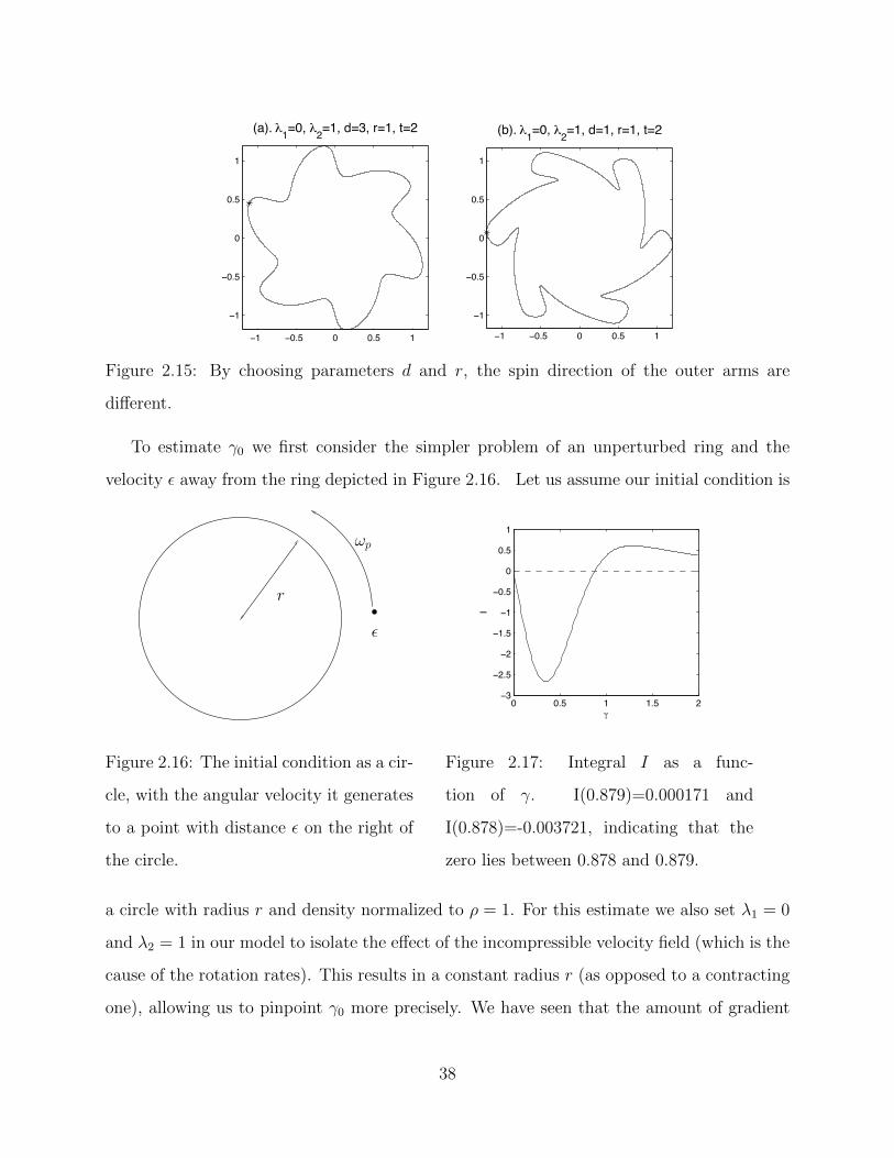
−1 −0.5 0 0.5 1

−1

−0.5

0

0.5

1

(a). λ1=0, λ2=1, d=3, r=1, t=2

−1 −0.5 0 0.5 1

−1

−0.5

0

0.5

1

(b). λ1=0, λ2=1, d=1, r=1, t=2

Figure 2.15: By choosing parameters d and r, the spin direction of the outer arms are

di↵erent.

To estimate �0 we first consider the simpler problem of an unperturbed ring and the

velocity ✏ away from the ring depicted in Figure 2.16. Let us assume our initial condition is

r

✏

!p

Figure 2.16: The initial condition as a cir-

cle, with the angular velocity it generates

to a point with distance ✏ on the right of

the circle.

0 0.5 1 1.5 2−3

−2.5

−2

−1.5

−1

−0.5

0

0.5

1

γ

I

Figure 2.17: Integral I as a func-

tion of �. I(0.879)=0.000171 and

I(0.878)=-0.003721, indicating that the

zero lies between 0.878 and 0.879.

a circle with radius r and density normalized to ⇢ = 1. For this estimate we also set �1 = 0

and �2 = 1 in our model to isolate the e↵ect of the incompressible velocity field (which is the

cause of the rotation rates). This results in a constant radius r (as opposed to a contracting

one), allowing us to pinpoint �0 more precisely. We have seen that the amount of gradient

38

in the kernel has an e↵ect on the rotational shearing but we will observe below that the

predicted �0 seems to be independent of �2.

To find the value of �0 we need to compute the angular velocity !p

of a point p = (1+✏, 0)

just outside the ring, i.e., where ✏⌧ 1; see Figure 2.16. This point represents a small radial

perturbation of the circle. If this point is moving faster than on the ring then perturbations

of the ring will result in spiral arms that shear in the counterclockwise direction relative to

the ring, as in example 2.15(b). If the point is moving slower than on the ring the spiral

arms will fall behind the ring, as in example 2.15(a). To calculate the angular velocity !p

of

the point p which is a distance ✏ from the circle we compute the integral

!p

=1

r + ✏

Z 2⇡

0

@x

Gd

(r + ✏� r cos ✓,�r sin ✓)rd✓. (2.36)

We then di↵erentiate (2.36) with respect to ✏ and we get to leading order

d!p

d✏=

2

d5· I, where I =

Z 2⇡

0

[�r

d2(1� sin ✓)2 +

d

rsin ✓]e�2(1�sin ✓) r

2

d2 d✓. (2.37)

We see that the sign of d!d✏ depends solely on � = r/d. When I < 0, i.e., d!

d✏ < 0, the

points on the arm which are closer to the circle have a faster angular velocity. Then the

arms appear to wind up in the opposite direction of the spin. When I > 0, i.e., d!

d✏

> 0, the

points on the arm which are outside the circle have a faster angular velocity, which makes

the arms appear to wind up in the same direction as the spin. Thus, our critical value �0 is

precisely when I(�0) = 0, which is the critical ratio of radius to kernel length scale. Figure

2.17 is a numerical calculation of I as a function of �. From this we see that �0 ⇡ 0.88 for

our example.

The existence of a critical �0 provides the explanation of why we see qualitatively di↵erent

dynamics in the spiral arms between Figure 2.15(a) and 2.15(b). Since the ratio r/d is what

determines the shearing behavior in our simpler problem, we can measure the accuracy of

�0 = 0.88 once we include both a nonzero �1 and �2 in our fully nonlinear perturbation

problem. By including a positive value for �1 the curve solution will attract toward the

origin. Thus, if we start with a ring whose large perturbations initially start outside of

39

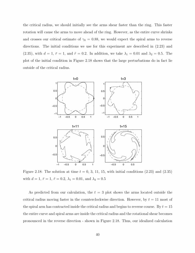
the critical radius, we should initially see the arms shear faster than the ring. This faster

rotation will cause the arms to move ahead of the ring. However, as the entire curve shrinks

and crosses our critical estimate of �0 = 0.88, we would expect the spiral arms to reverse

directions. The initial conditions we use for this experiment are described in (2.23) and

(2.35), with d = 1, r = 1, and r = 0.2. In addition, we take �1 = 0.01 and �2 = 0.5. The

plot of the initial condition in Figure 2.18 shows that the large perturbations do in fact lie

outside of the critical radius.

−1 −0.5 0 0.5 1−1

−0.5

0

0.5

1t=0

−1 −0.5 0 0.5 1−1

−0.5

0

0.5

1

t=3

−1 −0.5 0 0.5 1

−0.5

0

0.5

t=11

−0.5 0 0.5

−0.5

0

0.5

t=15

Figure 2.18: The solution at time t = 0, 3, 11, 15, with initial conditions (2.23) and (2.35)

with d = 1, r = 1, r = 0.2, �1 = 0.01, and �2 = 0.5

As predicted from our calculation, the t = 3 plot shows the arms located outside the

critical radius moving faster in the counterclockwise direction. However, by t = 11 most of

the spiral arm has contracted inside the critical radius and begins to reverse course. By t = 15

the entire curve and spiral arms are inside the critical radius and the rotational shear becomes

pronounced in the reverse direction - shown in Figure 2.18. Thus, our idealized calculation

40

for the critical radius based on the assumption of an unperturbed ring approximates the

reversal quite well, though it appears that the reversing of the spiral arm direction in the

t = 11 picture of Figure 2.18 does occur just outside of the ring.

41

CHAPTER 3

Stability of Ring Patterns in R2

3.1 Discrete and Continuum Models

In a general space dimension Rd, the N particle interaction system

dxj

dt=

1

N

X

k 6=j

f(|xj

� xk

|)(xj

� xk

), (3.1)

where rf(r) = �P 0(r) for some pairwise interaction potential P , is a gradient flow of the

energy

E(x1,x2, . . . ,xN

) =X

i,j 6=i

P (|xi

� xj

|). (3.2)

In a continuum limit as N ! 1, (3.1) takes the form of the aggregation equation

⇢t

(x, t) +r · (⇢(x, t)v(x, t)) = 0, with x 2 Rd,

v(x, t) =

Zf(x� y)(x� y)⇢(y, t)dy, (3.3)

which is also known as the active scalar equation. Here, ⇢ describes the density of particles

and v is the velocity field. By then considering a weak formulation of (3.3) where the

density aggregates on a co-dimension one shell one can derive, see [SUB, KSUB, VUKB] the

evolution equation for the material point of the shell, X(⇠), to be

Xt

= v =

Z

D

f(|X(⇠)�X(⇠0)|)(X(⇠)�X(⇠0))⇢0(⇠0)dS⇠0 , (3.4)

where parameterize the curve with Lagrangian parameter ⇠ 2 D ⇢ Rd�1.

42

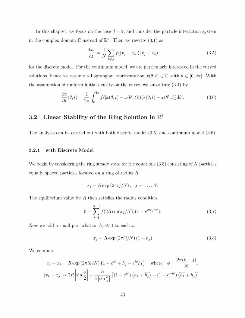
In this chapter, we focus on the case d = 2, and consider the particle interaction system

in the complex domain C instead of R2. Then we rewrite (3.1) as

dxj

dt=

1

N

X

k 6=j

f(|xj

� xk

|)(xj

� xk

) (3.5)

for the discrete model. For the continuum model, we are particularly interested in the curved

solutions, hence we assume a Lagrangian representation x(✓, t) 2 C with ✓ 2 [0, 2⇡]. With

the assumption of uniform initial density on the curve, we substitute (3.4) by

@x

@t(✓, t) =

1

2⇡

Z 2⇡

0

f(|x(✓, t)� x(✓0, t)|)(x(✓, t)� x(✓0, t))d✓0. (3.6)

3.2 Linear Stability of the Ring Solution in R2

The analysis can be carried out with both discrete model (3.5) and continuum model (3.6).

3.2.1 with Discrete Model

We begin by considering the ring steady state for the equations (3.5) consisting of N particles

equally spaced particles located on a ring of radius R,

xj

= R exp (2⇡ij/N) , j = 1 . . . N.

The equilibrium value for R then satisfies the radius condition

0 =N�1X

j=1

f(2R sin(⇡j/N))(1� ei2⇡j/N). (3.7)

Now we add a small perturbation hj

⌧ 1 to each xj

xj

= R exp (2⇡ij/N) (1 + hj

) (3.8)

We compute

xj

� xk

= R exp (2⇡ik/N)�1� ei� + h

j

� ei�hk

�where � =

2⇡(k � j)

N.

|xk

� xj

| ⇠ 2R

����sin�

2

����+R

4��sin �

2

��⇥(1� ei�)

�hk

+ hj

�+ (1� e�i�)

�hk

+ hj

�⇤.

43

Substituting (3.8) into (3.5) leads to the following linearized system,

dhj

dt=X

k

f 0✓2R

����sin�

2

����

◆R

4��sin �

2

�� [(1� ei�)�hk

+ hj

�

+ (1� e�i�)�hk

+ hj

�]�1� ei�

�

+X

k

f

✓2R

����sin�

2

����

◆ �hj

� ei�hk

�, where � =

2⇡(k � j)

N.

Next we use the identities

(1� ei�)2 = �4 sin2

✓�

2

◆ei�; (1� ei�)(1� e�i�) = 4 sin2

✓�

2

◆

to obtain

dhj

dt=X

k,k 6=j

G1(�/2)�hj

� ei�hk

�+G2(�/2)

�hk

� ei�hj

�,

where � =2⇡(k � j)

N

(3.9)

with

G1(�) =1

NRf 0 (2R |sin�|) |sin�|+ 1

Nf (2R |sin�|) ;

G2(�) =1

NRf 0 (2R |sin�|) |sin�| .

(3.10)

Use an anztaz

hj

= ⇠+(t)eim✓ + ⇠�(t)e

�im✓, ✓ = 2⇡j/N, m 2 N. (3.11)

Then

hk

= ⇠+eim✓eim� + ⇠�e

�im✓e�im�, (3.12)

and substituting (3.11), (3.12) into (3.9) and collecting like terms in eim�, e�im� leads to a

system

⇠0+ = ⇠+X

k,k 6=j

G1(�/2)�1� ei(m+1)�

�+ ⇠�

X

k,k 6=j

G2(�/2)�eim� � ei�

�(3.13)

⇠0� = ⇠�X

k,k 6=j

G1(�/2)�1� ei(�m+1)�

�+ ⇠+

X

k,k 6=j

G2(�/2)�e�im� � ei�

�(3.14)

It is easy to check that the sums in (3.13, 3.14) are all real so that the system becomes

⇠0+ = ⇠+I1(m) + ⇠�I2(m), ⇠0� = ⇠�I1(�m) + ⇠+I2(�m)

44

where

I1(m) =X

k,k 6=j

G1(�/2)�1� ei(m+1)�

�= 4

N/2X

k=1

G1(⇡k

N) sin2

✓(m+ 1) ⇡k

N

◆, (3.15)

I2(m) =X

k,k 6=j

G2(�/2)�eim� � ei�

�

= 4N/2X

k=1

G2(⇡k

N)

sin2

✓⇡k

N

◆� sin2

✓m⇡k

N

◆�. (3.16)

We thus obtain0

@ ⇠0+

⇠0

1

A = M ·0

@ ⇠+

⇠

1

A =

0

@ I1(m) I2(m)

I2(m) I1(�m)

1

A ·0

@ ⇠+

⇠

1

A (3.17)

Substituting ⇠± = b± exp (�t) we find that � is the eigenvalue of the matrix M.

3.2.2 with Continuum Model

The linear stability analysis for the ring solutions to the continuum model (3.6) is similar to

that of the discrete case. We start with the radius conditionZ ⇡

2

0

f(2R sin ✓) sin2 ✓d✓ = 0, (3.18)

which is a limit of (3.7) when N ! 1. Based on this, we assume the curved solution x(✓, t)

has a small deviation h(✓, t) ⌧ 1 from the ring steady state

x(✓, 0) = R exp (i✓)(1 + h(✓, 0)) (3.19)

In the rest of this chapter, for simplicity, we use the abbreviations x and x0 for x(✓, t) and

x(✓0, t), and h and h0 for h(✓, t) and h(✓0, t). We then have

x� x0 = R exp (i✓)�1� ei� + h� ei�h0� where � = ✓0 � ✓. (3.20)

|x� x0| ⇠ 2R

����sin�

2

����+R

4��sin �

2

��⇥(1� e�i�)

�h+ h0

�+ (1� ei�)

�h+ h0�⇤ . (3.21)

Substituting (3.20) and (3.21) into (3.6), with the same ansatz

h(✓, t) = ⇠+(t)eim✓ + ⇠�(t)e

�im✓, (3.22)

45

after similar analysis as in the discrete case, we arrive at the same linearization problem:

0

@ ⇠0+

⇠0

1

A = M ·0

@ ⇠+

⇠

1

A =

0

@ I1(m) I2(m)

I2(m) I1(�m)

1

A ·0

@ ⇠+

⇠

1

A , (3.23)

with I1(m), I2(m) defined as the limit of (3.15) and (3.16) when N ! 1. The above

discussion can be summarized into the following theorem.

Theorem 3.2.1. In the continuum model, consider the ring equilibrium of radius R given

by (3.18) for the flow (3.4). Define

I1(m) :=4

⇡

Z⇡/2

0

(Rf 0 (2R sin ✓) sin ✓ + f (2R sin ✓)) sin2((m+ 1)✓)d✓; (3.24)

I2(m) :=4

⇡

Z⇡/2

0

(Rf 0 (2R sin ✓) sin ✓)⇥sin2(✓)� sin2(m✓)

⇤d✓; (3.25)

M(m) :=

0

@ I1(m) I2(m)

I2(m) I1(�m)

1

A . (3.26)

Suppose that � 0 for all eigenvalues � of M(m) for all m 2 N. Then the ring equilibrium

is locally stable. It is unstable otherwise.

For finite N , the ring is stable if � 0 for all eigenvalues � of M(m) for all m =

1, 2, . . . N, but with I1, I2 as given by (3.15), (3.16).

3.2.3 Numerical Examples

In this section, we consider 2D particle interactions with specified interaction laws. In

particular, we consider a tanh kernel

f(r) =tanh((1� r)a) + b

r, (3.27)

and a power law kernel

f(r) = ra�1 � rb�1. (3.28)

A zoo of patterns arise if we plot the final steady states of the particle system (3.1) under

46

Figure 3.1: Simulation of (3.1) under interaction law (3.27) or (3.28) with certain parameter

choices on a and b.

interaction (3.27) with various parameter choices on a and b. In Figure 3.1, we observe pat-

terns such as rings, triangular curves, target, annulus, concentric rings, soccer ball pattern,

etc.

The evolution of the particle system (3.1) under interaction (3.27) or (3.28) with some

parameter choices are plotted in Figure 3.2. For the case where we simulate (3.1) and

(3.27), with a = 10, b = 0.1, as shown in the first row of Figure 3.2, we realize that there is a

mode two instability that distort the ring steady state into a more elliptical looking shape.

In addition, there seems to be another mode four instability that pushes the individuals

towards four high density groups. Indeed, one can apply Theorem 3.2.1 to mode m = 2, 4

and calculate the most positive eigenvalue of matrix M as defined in (3.26). As shown in the

left picture of Figure 3.3, both mode 2 and mode 4 leads to at least one positive eigenvalue

47

−1 0 1−1

0

1

−1 0 1−1

0

1

−1 0 1−1

0

1

−1 0 1−1

0

1

−1 0 1−1

0

1

−1 0 1−1

0

1

−1 0 1−1

0

1

−1 0 1−1

0

1

−1 0 1−1

0

1

−1 0 1−1

0

1

−1 0 1−1

0

1

−1 0 1−1

0

1

Figure 3.2: Simulation of (3.1) under interaction law (3.27) or (3.28) with certain parameter

choices. Simulation size: N = 400 individuals. First column, t = 0; Second column, t = 2;

Third column, t = 50; Forth column, t = 1000. First row, tanh kernel (3.27), with a = 10,

b = 0.1; Second row, power law kernel (3.28), with a = 0.5, b = 6; Third row, power law

kernel (3.28), with a = 0.5, b = 4.

for M , and hence are unstable. Interestingly, we also observe instability for many other

modes.

For the cases where we simulate (3.1) and (3.28), we have two examples plotted in Figure

3.2, one with a = 0.5, b = 6, with ring solution bifurcates into a three mode instability,

another with a = 0.5, b = 4, with ring solution a stable steady state. The corresponding

calculations of the most positive eigenvalues of M as plotted in Figure 3.3 suggest that mode

3 is unstable when a = 0.5, b = 6, and stable when a = 0.5, b = 4. These results coincide

with the numerical simulations.

48

0 5 10 15 20−0.5

0

0.5

1

0 5 10 15 20−0.6

−0.4

−0.2

0

0.2

0 5 10 15 20−0.4

−0.3

−0.2

−0.1

0

Figure 3.3: The most positive eigenvalue of M(m) as defined in (3.26), for modes m ranging

from 1 to 20. Left: tanh kernel (3.27), with a = 10, b = 0.1; Middle: power law kernel (3.28),

with a = 0.5, b = 6; Right: power law kernel (3.28), with a = 0.5, b = 4.

3.3 Linear Stability of the Shell Solution in Rd

A generalization of the linear stability theory of the shell solution in Rd with d � 3 is derived

by Brecht et. al.[VUKB]. The analysis utilizes spherical harmonics and hypergeometric

functions. In this section, we present their results without proving it. Hereby we denote a

unit spherical shell as Sd�1. Recall that in Rd, the distance between two vectors on a sphere

|X�X0| can be related to their inner product through the following formula:

|Y �Y0|2/2 = R2 �Y ·Y0, given |Y| = |Y0| = R. (3.29)

For convenience, we rewrite (3.4) as

Yt

= v =

Z

D

g

✓ |Y �Y0|22

◆(Y �Y0)dS⇠0 , (3.30)

where g

✓ |Y �Y0|22

◆= f(|Y �Y0|). (3.31)

We then denote the unit sphere as: B(⇠)e1, where B serves as a rotation matrix, e1 is a unit

vector (1, 0, · · · , 0) in Rd, and ⇠ is a parameterization of the unit sphere. The columns of the

matrix B = [b1, b2, · · · , bd] can be defined as the following: b1 is the position on the sphere,

bj

= b1⇠j�1

, the derivative of b1 with respect to ⇠j�1, and b

j

= bj

/|bj

| for 2 j d. The

49

perturbed solution can be written as:

Y(⇠) = B(⇠) · (Re1 + �(⇠)e�t), (3.32)

�(⇠) = ✏[c1Sm(⇠), c2

Sm

⇠1(⇠)

|b1|, · · · , c2

Sm

⇠d�1(⇠)

|bd�1|

], (3.33)

where R satisfies the radius condition:

Z 1

�1

g(R2(1� s))(1� s)(1� s2)d�32 ds = 0, (3.34)

and Sm is a spherical harmonic of mode m. Through the definition of B, we notice that c1

corresponds to the perturbation in the normal direction and c2 corresponds to the perturba-

tion in the tangential direction of the shell. Because of the spherical symmetry of the shell,

all tangential directions are equivalent.

The linearization of the shell solution to system (3.30) can be formulated as a scalar

eigenvalue problem[VUKB]:

�

2

4c1

c2

3

5 = Md

(m)

2

4c1

c2

3

5 =

2

4↵ + �d,m

(g1) m(d+m� 2)�d,m

(g2)

�d,m

(g2) m(d+m� 2)�d,m

(g3)/R2

3

5

2

4c1

c2

3

5 , (3.35)

with ↵ = vol(Sd�2)

Z 1

�1

(1� s2)d�32 · �g(R2(1� s)) +R2g0(R2(1� s))(1� s)2

�ds,

g1(s) = R2g0(R2(1� s))(1� s)2 � g(R2(1� s))s,

g2(s) = g(R2(1� s))(1� s), and g03(s) = �R2g(R2(1� s)). (3.36)

Here, m denotes the mode of the spherical harmonic and, for any function h smooth enough,

�d,m

(h) = vol(Sd�2)

Z 1

�1

h(s)P(d/2�1)

m

(s)(1� s2)d�32 ds, (3.37)

where P(d/2�1)

m

are Gegenbauer polynomials[S2], normalized so that Pm

(1) = 1.

The shell solution with radius R defined by (3.34) is linearly stable if � < 0 for all the

eigenvalues of Md

(m); it is unstable with mode m perturbation if � > 0 for one of the two

eigenvalues of Md

(m).

50

3.4 Weakly Nonlinear Analysis: Low Mode Bifurcations

Theorem 3.2.1 characterizes the conditions for a ring solution to be stable for the continuum

model. That is, the eigenvalues of the matrix M(m) defined in (3.26) should be both

nonpositive. For a given mode m, when one of the eigenvalues becomes zero, the stability

changes. In this section, we study the bifurcation dynamics in general using weakly nonlinear

analysis. As such, we rewrite the continuum model (3.6):

@x

@t(✓, t) =

1

2⇡

Z 2⇡

0

f(⌫, |x(✓, t)� x(✓0, t)|)(x(✓, t)� x(✓0, t))d✓0, (3.38)

where ⌫ is considered to be the bifurcation parameter. We are particularly interested in the

critical value of ⌫, i.e. ⌫ = ⌫0, which gives zero determinant ofM(m), with the corresponding

ring steady state solution

x(✓, t) = u0(✓, t) = Rei✓. (3.39)

For simplicity, in the rest of this section, we use the notation x for x(✓, t), x0 for x(✓0, t), f

for f(⌫0, |x(✓, t) � x(✓0, t)|), @⌫

f for @f/@⌫ evaluated at (⌫0, |x(✓, t) � x(✓0, t)|), and f 0, f 00,

etc. for the corresponding derivatives of f with respect to the second argument evaluated at

(⌫0, |x(✓, t) � x(✓0, t)|). Let 0 ✏ ⌧ 1 be an expansion parameter near a bifurcation point

u0,

x(✓, t) = u0(✓, t) + ✏u1(✓, t) + ✏2u2(✓, t) + ✏3u3(✓, t) + · · · , (3.40)

⌫ = ⌫0 + ✏⌫1 + ✏2⌫2 + · · · . (3.41)

At order O(✏), we obtain the linear equation

L(u1, u1) =1

⇡

Z⇡

0

(f 0R sin�+ f)(u1 � u01)d�

� e2i✓

⇡

Z⇡

0

f 0R sin�e2i�(u1 � u01)d�

=� ⌫1I0ei✓, with I0 =

4

⇡

Z⇡/2

0

R@⌫

f sin2 �d�

(3.42)

and � = (✓0 � ✓)/2. The solution to (3.42) is u1 = b1ei(m+1)✓ + b2e

�i(m�1)✓ + b0ei✓, where

[b1, b2]t 2 N (M(m)) and b0 = ⌫1c1, with c1 = �I0/(I1(0) + I2(0)). This is the eigenvalue

51

problem for the linear stability of the ring solution. Typically one measures the amplitude

that the solution deviates either radially as |b2 + b1| or tangentially as |b2 � b1|.At order O(✏2), we obtain

L(u2, u2) =

� ⌫1 (b1, b2) ·0

@ 2c1I3(m) + @⌫

I1(m) �2c1I4(m) + @⌫

I2(m)

�2c1I4(m) + @⌫

I2(m) 2c1I3(�m) + @⌫

I1(�m)

1

A ·0

@ ei(m+1)✓

e�i(m�1)✓

1

A

�0

@ b21I5(m) + b22I6(m)� b1b2I7(m)

b21I5(�m) + b22I6(�m)� b1b2I7(�m)

1

At

·0

@ ei(2m+1)✓

e�i(2m�1)✓

1

A

�✓⌫2I0 +

⌫212@⌫

I0 +�b1b2I4(m) + b21I3(m) + b22I3(�m)

�◆ei✓,

(3.43)

where

I3(m) =4

⇡

Z⇡/2

0

(2Rf 00 sin�+ 3f 02(m+ 1)� sin�d�,

I4(m) =4

⇡

Z⇡/2

0

(2Rf 00 sin�+ f 0) sin (m� 1)� sin (m+ 1)� sin�d�,

I5(m) =2

⇡

Z⇡/2

0

(3

2f 0 +Rf 00 sin�) sin2 (m+ 1)� sin (2m+ 1)�d�,

I6(m) =2

⇡

Z⇡/2

0

(�1

2f 0 +Rf 00 sin�) sin2 (m� 1)� sin (2m+ 1)�d�,

I7(m) =2

⇡

Z⇡/2

0

(3f 0 + 2Rf 00 sin�) sin (m� 1)� sin (m+ 1)� sin (2m+ 1)�d�.

Applying the Fredholm alternative to ensure that the right hand side of (3.43) is in the

range space of the linear operator L determines a unique solution u2 = b21c3ei(2m+1)✓ +

b21c4e�i(2m�1)✓ + (⌫2c1 + b21c2)e

i✓, subject to the condition that ⌫1 = 0, where

c2 = ��I1(m)I4(m)/I2(m) + I3(m) + I1(m)2I3(�m)/I2(m)2

I1(0) + I2(0),

2

4 c3

c4

3

5 = �M(2m)�1 ·2

4 I5(m) + I1(m)2I6(m)/I2(m)2 + I1(m)I7(m)/I2(m)

I5(�m) + I1(m)2I6(�m)/I2(m)2 + I1(m)I7(�m)/I2(m)

3

5

(3.44)

52

Finally, at O(✏3), we use the equation L(u3, u3) = R3(u0, u1, u2, ⌫2), to determine the rela-

tion between ⌫2 and b1, b2. Applying the Fredholm alternative to this equation,

Im�R3(u0, u1, u2, ⌫2)(I1(m)e�i(m+1)✓ + I2(m)ei(m�1)✓)

�= 0, (3.45)

which yields

⌫2 = b21

=⌧4I1(m)I2(m)� ⌧3I2(m)2

⌧1I2(m)� ⌧2I1(m) + I2(m)2@⌫

I1(m)� 2I1(m)I2(m)@⌫

+ I1(m)2@⌫

I1(�m), (3.46)

where

⌧1 = 2c1I2(m)I8(m) + 2c1I1(m)I9(m)

⌧2 = �2c1I1(m)I8(�m)� 2c1I2(m)I9(m)

⌧3 = 2c2I8(m) + 2c2I1(m)I9(m)/I2(m)

+ c3I1(m)I11(m)/I2(m) + c3I10(m) + c4I1(m)I11(�m)/I2(m) + c4I12(�m)

+ I14(m) + I1(m)I15(m)/I2(m) + I1(m)2I16(m)/I2(m)2 + I1(m)3I13(�m)/I2(m)3

⌧4 = �2c2I1(m)I8(�m)/I2(m)� 2c2I9(m)

� c4I11(�m)� c4I1(m)I10(�m)/I2(m) + c3I1(m)I11(m)/I2(m) + c3I12(m)

� I1(m)3I14(�m)/I2(m)3 � I1(m)2I15(�m)/I2(m)2 � I1(m)I16(�m)/I2(m)� I13(m)

(3.47)

53

and

I8(m) =2

⇡

Z⇡/2

0

(2Rf 00 sin�+ 3f 0) sin2 (m+ 1)� sin�d�,

I9(m) =2

⇡

Z⇡/2

0

(2Rf 00 sin�+ f 0) sin (m� 1)� sin (m+ 1)� sin�d�,

I10(m) =2

⇡

Z⇡/2

0

(2Rf 00 sin�+ 3f 0) sin2 (m+ 1)� sin (2m+ 1)�d�,

I11(m) =2

⇡

Z⇡/2

0

(2Rf 00 sin�+ 3f 0) sin (m� 1)� sin (m+ 1)� sin (2m+ 1)�d�,

I12(m) =2

⇡

Z⇡/2

0

(2Rf 00 sin�+ f 0) sin2 (m� 1)� sin (2m+ 1)�d�,

I13(m) =2

⇡

Z⇡/2

0

(2Rf 000 sin�+ 3f 00 � 3f 0

2R sin�) sin (m� 1)� sin3 (m+ 1)�d�✓,

I14(m) =2

⇡

Z⇡/2

0

(2Rf 000 sin�+ 5f 00 +3f 0

2R sin�) sin4 (m+ 1)�d�,

I15(m) =2

⇡

Z⇡/2

0

(5

3Rf 000 sin�+ 2f 00 � f 0

R sin�) sin3 (m+ 1)� sin (m� 1)�d�,

I16(m) =2

⇡

Z⇡/2

0

(5

3Rf 000 sin�+ 2f 00 +

f 0

R sin�) sin2 (m� 1)� sin2 (m+ 1)�d�.

(3.48)

We conclude this section with the following theorem:

Theorem 3.4.1. Let f(⌫, r) be an attractive-repulsive kernel, with a parameter ⌫, where

mode m perturbation is stable for ⌫ < ⌫0, unstable for ⌫ > ⌫0 and f(⌫0, r) gives the instability

threshold det(M(m)) = 0. Given the following conditions:

1. I0 6= 0

2. I1(0) + I2(0) 6= 0

3. The matrix N(m) =

0

@ 2c1I3(m) + @⌫

I1(m) �2c1I4(m) + @⌫

I2(m)

�2c1I4(m) + @⌫

I2(m) 2c1I3(�m) + @⌫

I1(�m)

1

A has nonzero

determinant.

4. The matrix M(2m) has nonzero determinant.

54

5. The denominator of in (3.46) is nonzero.

Then we have a pitchfork bifurcation for solutions of (3.38) at ⌫ = ⌫0, with bifurcation

coe�cient defined either

⌫2/|b1 + b2|2 = I2(m)2/(I1(m)� I2(m))2 (radially),

or ⌫2/|b1 � b2|2 = I2(m)2/(I1(m) + I2(m))2 (tangentially),

where ⌫2 and are defined in (3.46).

3.4.1 Numerical Example

Figure 3.4: Bifurcation diagram for interaction force (3.28), with p = 0.5. The solid curve is

calculated from Theorem 3.4.1.

We now use weakly nonlinear theory to analyze how the transition of stability occurs.

Figure 3.4 is a bifurcation diagram for interaction force (3.28), taking p = 0.5, where we

record the change of the quantity

�r = rmax

� rmin

according to the bifurcation parameter q, with rmax

and rmin

being the maximum and min-

imum of the displacement from the origin. Numerical simulation for the whole system (3.1)

are done with 100 particles with random initial condition, plotted as black dots. At q = 4.95

the steady state solution remains a stable ring; while at q = 4.98 the mode 3 becomes slightly

55

unstable and the points tend to move tangentially to break the ring into a triangular shape.

By further increasing q, the points on the curve continue to move toward a more triangular

shape. The weakly nonlinear analysis confirms that this process is in fact a supercritical

pitchfork bifurcation. We apply Theorem 3.4.1 to obtain the analytical form of the pitchfork

�r =pmax{0, ⌧ · (q � q

c

)} with qc

⇡ 4.9696 and ⌧ ⇡ 0.01188, (3.49)

which is plotted as a solid line in 3.4.

56

CHAPTER 4

Stability of Cluster Patterns in Rd

In this chapter we consider the clusters problem

Yj

= v =1

N

X

k 6=j

f(|Yj

�Yk

|) Yj

�Yk

|Yj

�Yk

|mk

(4.1)

in Rd for both d = 2 and d > 2. Given n particles in Rd, m clusters may form under a

given interaction force f when we impose the condition that n

m

2 N. Let us denote the

cluster configuration as {pd,1,p

d,2, . . . ,p

d,m}, and order the particles gathering in the ith

cluster pd,i

as Yi,j

, with j 2 {1, 2, . . . , n

m

}. In two dimensions, the positions of the clusters

p2,i will be equally distributed on the ring (see the statement of Theorem 4.1.1). Thus for

our stability analysis we consider perturbations ✏i,j on each particle such that Yi,j , so that

Yi,j = pi,j + ✏i,j .

4.1 Stability of Clusters in R2

We begin by summarizing in Theorem 4.1.1 the stability of clusters in R2 for a general

interaction kernel, f , which we then prove in the remainder of this section.

Theorem 4.1.1. Consider the discrete cluster problem (4.1) in R2 and let r satisfy the

radius condition

mX

k=1

f(2r sin⇡k

m) sin

⇡k

m= 0, (4.2)

then the m cluster configuration p2,k

=�r cos 2⇡k

m

, r sin 2⇡km

�with n

m

2 Z particles in each

cluster is stable if and only if the following two conditions are satisfied:

57

1. c? 0 and c

k 0, with c?and c

kdefined below in (4.3).

c?=

1

m

mX

k

0=1

(

f 0(2r sin ⇡k

0

m

)

2

+

f(2r sin ⇡k

0

m

)

4r sin ⇡k

0m

)

�(

f 0(2r sin ⇡k

0

m

)

2

� f(2r sin ⇡k

0

m

)

4r sin ⇡k

0m

) cos

2⇡k0

m

!,

ck=

1

m

mX

k

0=1

(

f 0(2r sin ⇡k

0

m

)

2

+

f(2r sin ⇡k

0

m

)

4r sin ⇡k

0m

)

+(

f 0(2r sin ⇡k

0

m

)

2

� f(2r sin ⇡k

0

m

)

4r sin ⇡k

0m

) cos

2⇡k0

m

!. (4.3)

2. The matrix A(l) with entries A11(l), A12(l), A21(l), A22(l) defined below in (4.4) is

non-positive definite for l 2 {0, 1, 2, . . . , ⇥m�12

⇤}.

A11(l) = A22(�l)

=

1

m

mX

k

0=1

(

f 0(2r sin ⇡k

0

m

)

2

+

f(2r sin ⇡k

0

m

)

4r sin ⇡k

0m

)(1� cos

2⇡k0(l + 1)

m),

A12(l) = A21(l)

=

1

m

mX

k

0=1

(�f 0(2r sin ⇡k

0

m

)

2

+

f(2r sin ⇡k

0

m

)

4r sin ⇡k

0m

)(cos

2⇡k0

m� cos

2⇡k0l

m). (4.4)

We prove this by classifying the cluster instabilities that may occur into two types. The

first kind of instability comes from fixing the center of mass for each cluster. Since each

particle has two principle directions of freedom, the tangential and radial directions, and

fixing the center of mass in both directions reduces two degrees of freedom for each cluster,

the total degrees of freedom for the first kind of instability is 2(n � m). The second kind

of instability comes in by considering the stability of centers of mass for the clusters by

regarding each cluster as a single particle, introducing another 2m degrees of freedom which

brings the total degrees of freedom to 2n which is the dimension of the problem. We will

classify the stability of each of these types of instabilities to prove theorem 4.1.1 .

Proof. Let ✏?k,j

represent the normal perturbation, and ✏kk,j

represent the tangential pertur-

58

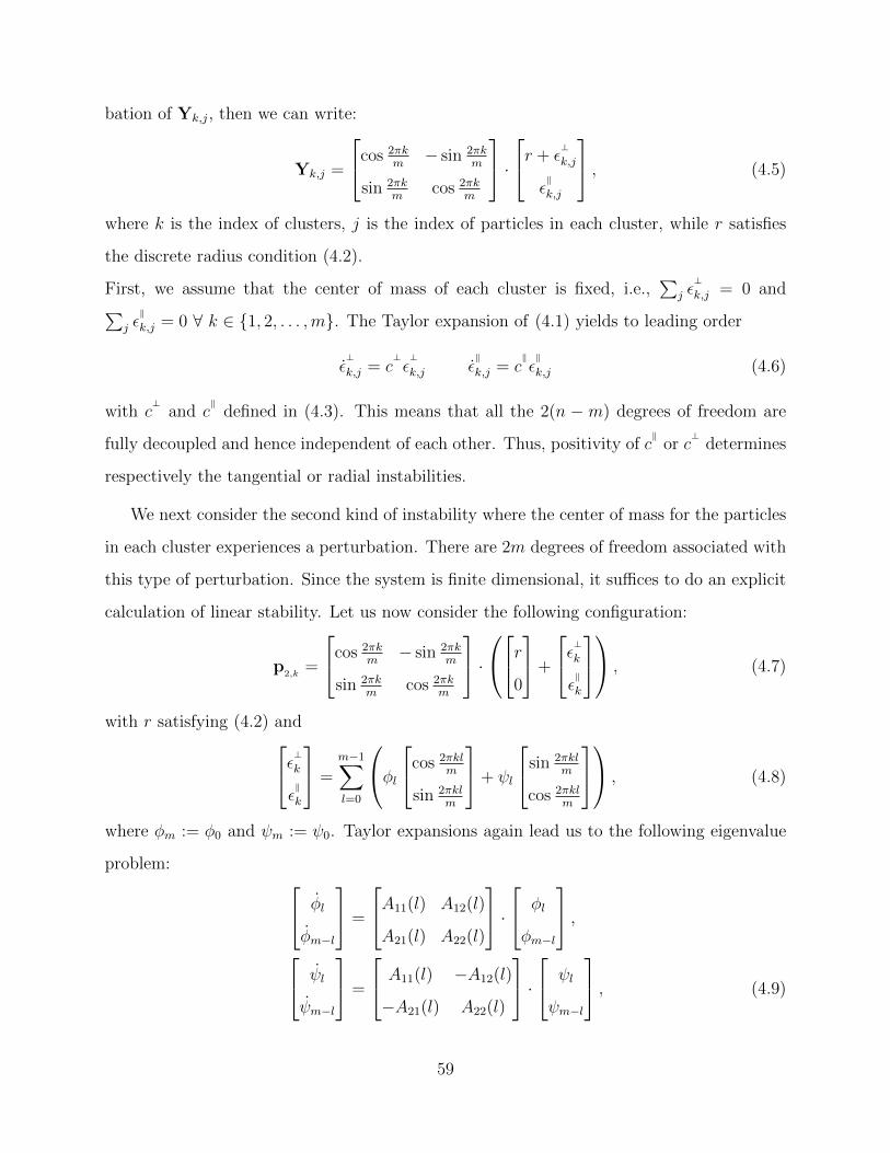
bation of Yk,j

, then we can write:

Yk,j

=

2

4cos2⇡km

� sin 2⇡km

sin 2⇡km

cos 2⇡km

3

5 ·2

4r + ✏?k,j

✏kk,j

3

5 , (4.5)

where k is the index of clusters, j is the index of particles in each cluster, while r satisfies

the discrete radius condition (4.2).

First, we assume that the center of mass of each cluster is fixed, i.e.,P

j

✏?k,j

= 0 andP

j

✏kk,j

= 0 8 k 2 {1, 2, . . . ,m}. The Taylor expansion of (4.1) yields to leading order

✏?

k,j

= c?✏?

k,j

✏k

k,j

= ck✏k

k,j

(4.6)

with c?and c

kdefined in (4.3). This means that all the 2(n � m) degrees of freedom are

fully decoupled and hence independent of each other. Thus, positivity of ckor c

?determines

respectively the tangential or radial instabilities.

We next consider the second kind of instability where the center of mass for the particles

in each cluster experiences a perturbation. There are 2m degrees of freedom associated with

this type of perturbation. Since the system is finite dimensional, it su�ces to do an explicit

calculation of linear stability. Let us now consider the following configuration:

p2,k

=

2

4cos2⇡km

� sin 2⇡km

sin 2⇡km

cos 2⇡km

3

5 ·0

@

2

4r

0

3

5+

2

4✏?k

✏kk

3

5

1

A , (4.7)

with r satisfying (4.2) and2

4✏?k

✏kk

3

5 =m�1X

l=0

0

@�l

2

4cos2⇡klm

sin 2⇡klm

3

5+ l

2

4sin2⇡klm

cos 2⇡klm

3

5

1

A , (4.8)

where �m

:= �0 and m

:= 0. Taylor expansions again lead us to the following eigenvalue

problem:2

4 �l

�m�l

3

5 =

2

4A11(l) A12(l)

A21(l) A22(l)

3

5 ·2

4 �l

�m�l

3

5 ,

2

4 l

m�l

3

5 =

2

4 A11(l) �A12(l)

�A21(l) A22(l)

3

5 ·2

4 l

m�l

3

5 , (4.9)

59

with l 2 {0, 1, . . . ⇥m�12

⇤}, where A11(l), A12(l), A21(l), A22(l) are defined in (4.4). Thus, a

necessary and su�cient condition for the second kind of stability is that A(l) is non-positive

definite with l 2 {0, 1, . . . ⇥m�12

⇤}. This completes the proof of Theorem 4.1.1.

Remark 1 (Remark). The two dimensional linear systems in (4.9) reduce to one dimension

in certain cases. For the case l = m

2 with m even or l = 0, we have l = m � l and hence

�l

= �m�l

, l

= m�l

. Furthermore, we have A11(l) = A22(l) and A12(l) = A21(l). Hence

(4.9) becomes �l

= (A11(l) + A12(l))�l

and l

= (A11(l)� A12(l)) l

, and the condition that

A11(l) +A12(l) 0 and A11(l)�A12(l) 0 is equivalent to A(l) being non-positive definite.

When l = 0, it is a direct verification that A11(l) + A12(l) < 0 and A11(l) � A12(l) = 0,

corresponding to our intuition that the expansion is stable and rotation is neutrally stable.

4.2 Stability of Clusters in General Space Dimensions

The argument of cluster stability in R2 does not extend to a higher dimensional space Rd

with m clusters. However, we may consider a simple case, in which we study the linear

stability of a simplex configuration.

Let us define the vertices of a simplex in general space dimension in the following sequen-

tial way: We begin by writing the vertices of an equilateral triangle as the following three

points:

p2,1 =(r, 0), p2,2 = (r cos ✓2, r sin ✓2),

p2,3 = (r cos ✓2,�r sin ✓2), (4.10)

with ✓2 = 2⇡/3. We can naturally express the vertices of a tetrahedron using this notation

as the following four points:

p3,1 = (r, 0, 0), p3,2 = (r cos ✓3, sin ✓3p2,1),

p3,3 =(r cos ✓3, sin ✓3p2,2), p3,4 = (r cos ✓3, sin ✓3p2,3), (4.11)

with ✓3 = arccos(�13). Let us call the vertices of an equilateral triangle p2 := {p2,1 ,p2,2 ,p2,3}

a simplex in R2, and the vertices of a regular tetrahedron p3 := {p3,1 ,p3,2 ,p3,3 ,p3,4} the

60

vertices of a simplex in R3. In higher dimensions we have the following recursive relation for

pi,j :

pi,1 = (r, 0, · · · , 0),pi,j = (r cos(✓

i

), sin(✓i

)pi�1,j�1) for j � 2, (4.12)

where ✓i

= arccos(�1i

). It is easy to verify that:

pi,j

|pi,j |· p

i,j0

|pi,j0 |

= �1

ifor j 6= j0. (4.13)

and we set pi := {pi,1 , . . . ,pi,i+1} to be the vertices of a simplex in Ri. Notice that for the

vertices of a simplex to be a steady state for (4.1), we need the distance � between any

two points pi,j and pi,j0 to be exactly the zero of f . We summarize this discussion in the

following definition.

Definition 4.2.1 (Definition). A simplex configuration solution is a configuration with

clusters {pd,1,p

d,2, . . . ,p

d,d+1} as vertices of a simplex with inter-vertex distance � > 0 where

f(�) = 0. We also enforce that at each cluster pd,i

there are an equal number particles

{Yi,j

, j 2 {1, 2, . . . , n

m

}}.

Given this definition we can now write our perturbation ansatz of our simplex solution

as:

✏i,j = Yi,j

� pd,i.

We now state our main result which is that it is enough to just study the stability in R2 to

classify the stability of simplex solutions in Rd.

Theorem 4.2.2. Consider the cluster problem (4.1) in Rd, the simplex configuration solution

is a stable configuration if and only if the following two conditions are satisfied:

1. The simplex configuration in R2 is stable under tangential perturbations ✏i,j with

X

j

✏i,j = 0, 8i.

61

2. f 0(0) + d+12 f 0(�) 0.

Remark 2 (Remark). Recall that f being repulsive at short distance and attractive at long

distance implies that there is only one non-zero root of f . Thus condition 2 of Theorem 4.2.2

is well-defined.

To prove the above theorem, we make use of the following three lemmas:

Lemma 4.2.3. The simplex configuration in Rd, d > 2 is stable under tangential perturba-

tions ✏i,j of particles Yi,j withP

j

✏i,j = 0 8 i () the simplex configuration in R2 under

tangential perturbations of each particle Yi,j withP

j

✏i,j = 0 8 i.

Lemma 4.2.4. The simplex configuration in Rd is stable under normal perturbations of

particles Yi,j withP

j

✏i,j = 0 8i () 2f 0(0) + (d+ 1)f 0(�) 0.

Lemma 4.2.5. The simplex configuration in Rd is always stable under perturbations to the

positions of each cluster pd,j.

We first provide a short proof of Theorem 4.2.2 and then prove Lemmas 4.2.3-4.2.5.

Proof of Theorem 4.2.2: A general perturbation of the simplex configuration Yi,j can be

decomposed into three parts: The first being tangential perturbations with the center of

mass for each cluster fixed, i.e,P

j

✏i,j = 0 or equivalently d+1n

Pj

Yi,j = pd,i, which have

(d�1)(n�d�1) degrees of freedom; the second being normal perturbations with the center

of mass for each cluster fixed, i.e, d+1n

Pj

Yi,j = pd,i, which have n�d�1 degrees of freedom;

and finally the third being perturbations of clusters pd,i, having d(d+1) degrees of freedom.

These three kinds of perturbations are orthogonal to one another and exhaust all the nd

degrees of freedom. The third kind of perturbation always decays because of Lemma 4.2.5

and the first and second kinds of perturbations are considered in Lemmas 4.2.3 and 4.2.4,

which give the necessary and su�cient conditions for the simplex configuration to be stable

in Theorem 4.2.2.

62

p3,1

p3,2

p3,3

p3,4

c1

c2

p3,1 p3,2

p3,3

p3,4

c1

c2

oo

Figure 4.1: regular tetrahedron on sphere

Proof of Lemma 4.2.3: To prove that the tangential perturbations of the simplex configura-

tion in R2 withP

j

✏i,j = 0 8 i are stable () the tangential perturbations of the simplex

configuration in Rd withP

j

✏i,j = 0 8 i are stable for any d, it is enough to prove the

following induction statement:

8 d � 2, the tangential perturbations of the simplex configuration in Rd withP

j

✏i,j = 0

8 i are stable () the tangential perturbations of the simplex configuration in Rd+1 withP

j

✏i,j = 0 8 i are stable.

For simplicity, we prove the above statement for the base case d = 2, as the inductive

step follows similarly to this argument. A simplex configuration in d = 3, as shown in

Figure 4.1, is constructed by adding to an equilateral triangle configuration {p3,2 ,p3,3 ,p3,4} a

cluster p3,1 (in d = 2) whose projection is right on the center of the triangle {p3,2 ,p3,3 ,p3,4},with the distance between p3,1 and p3,i being � 8 i 2 {2, 3, 4}, and then enforcing that

the number of particles in each cluster to be n

4 2 R. A general tangential perturbation

{✏i,j , i 2 {1, 2, 3, 4}, j 2 {1, 2, . . . , n4}} withP

j

✏i,j = 0 can be written as a linear composition

of tangential perturbations to the ith cluster {✏i,j , j 2 {1, 2, . . . , n4}}. So our task is now to

consider the stability of perturbations of the ith cluster withP

j

✏i,j = 0 and ✏i0,j = 0 8 i0 6= i.

To classify the stability let us return our attention to Figure 4.1 and the case i = 1 for

simplicity. Let us consider the tangential perturbations {✏1,j , i 2 {1, 2, . . . , n4}} on the point

63

p3,1 , withP

✏1,j = 0. We can further decompose ✏1,j uniquely into a tangential component

✏11,j

in the plane determined by three points p3,1 , p3,2 , p3,3 and a tangential component ✏21,j

in the plane determined by three points p3,1 , p3,3 , p3,4 . The magnitude of the perturbation

✏11,j

satisfies equation (4.6) with ck determined by (4.3) and, by Taylor expanding (4.1), the

perturbation ✏11,j

has a higher order therefore negligible e↵ect on particles Y4,j located at

the point p3,4 . Thus any perturbation {✏1,j = ✏11,j, ✏

i0,j = 0, 8i0 6= 1} with arbitrary ✏11,j

andP

j

✏11,j

= 0 is an eigenvector of the linearization of (4.1) with eigenvalue ck. The same

analysis applies for ✏21,j. In general, by analyzing perturbations {✏i,j , j 2 {1, 2, . . . , n4}} for

i 2 {2, 3, 4} similarly, we find that ✏i,j satisfies the following:

✏i,j = ck✏i,j , (4.14)

with ck determined by (4.3). In another word, any perturbation {✏i,j , i 2 {1, 2, 3, 4}, j 2{1, 2, . . . , n4}} with

Pj

✏i,j = 0 8 i is an eigenvector of the linearization of (4.6) with eigen-

value ck. The value ck as calculated for m = 3 in R2 is f 0(0)f0(�)2 . This completes the base

case of d = 2.

The induction in higher dimensions is proved similarly by adding a single new point

orthogonally to the lower dimensional simplex and then showing that the original simplex

has a higher order e↵ect on the tangential linear stability of the new vertex. The details are

left to the reader. We can thus conclude that the sign of f 0(0)+ f

0(�)2 determines the stability

of tangential perturbations in Rd withP

j

✏i,j = 0 for all d � 2.

Proof of Lemma 4.2.4. Consider the simplex configuration {pd,i

: i 2 {1, . . . , d + 1}} in

Rd with n

d+1 2 N particles {Yi,j

, j 2 {1, 2, . . . , n

d+1}} in each pd,i. Let us now consider

perturbations in the normal direction ✏i,j = ✏i,jpd,i

|pd,i |to the point Y

i,j

. The leading order

interaction of particle Yi0,j0 from particle Yi,j is 1

n

f 0(�)q

d+12d (✏

i,j

+ ✏i

0,j

0)pd,i�p

d,i0

|pd,i�pd,i0 |

. Un-

der the assumption thatP

j

0 ✏i0,j0 = 0 8 i0, we have that by summing over j0 the total

leading order interaction of particles {Yi0,j0 , j

0 2 {1, 2, . . . , n

d+1}} of pd,i0 on particle Yi,j is

1d+1f

0(�)q

d+12d ✏i,j

pd,i�pd,i0

|pd,i�pd,i0 |

. If we now sum over all i0 6= i the total leading order interaction of

all the particles {Yi0,j0 , j

0 2 {1, 2, . . . , n

d+1}} on the particleYi,j as12f

0(�)✏i,j

pd,i

|pd,i |. We can also

64

easily compute the leading order interaction of all the particles {Yi,j0 , j

0 2 {1, 2, . . . , n

d+1}}in the same cluster p

d,iof particle Yi,j is 1

d+1f0(0)✏i,j

pd,i

|pd,i |. Combing all of the above leading

order interactions {Yi0,j0 , j

0 2 {1, 2, . . . , n

d+1}} has on Yi,j , we arrive at the following:

✏i,j =2f 0(0) + (d+ 1)f 0(�)

2(d+ 1)✏i,j . (4.15)

Thus, Lemma 4.2.4 is proved.

Proof of Lemma 4.2.5: We consider perturbations to the center of mass of each cluster pd,i.

In this case we need not study the dynamics of each individual particle but instead the

interactions between the clusters pd,i. This configuration is analogous to a spring system,

with a spring joining each pair pd,i

and pd,i0 . Given that f is short range repulsive and long

range attractive, each such spring has a spring constant of � 1d+1f

0(�) > 0, and the spring

force of pd,i0 on p

d,ito leading order is 1

d+1f0(�)(|p

d,i�p

d,i0 |��)pd,i�p

d,i0

|pd,i�pd,i0 |

. We can therefore

define the energy of this system to leading order as

E(pd,1,p

d,2, . . . ,p

d,d+1)

=� 1

2

X

i

0 6=i

f 0(�)

d+ 1(|p

d,i� p

d,i0 |� �)2. (4.16)

It is now straightforward to check that (4.1) to leading order is a system that describes the

gradient flow of the energy as defined by (4.16). Thus the system settles down to a local

minima of E, which is exactly the simplex configuration.

65

CHAPTER 5

Stability and Clustering of Self-Similar Solutions to

Aggregation Equations

In this chapter we investigate the self-similar solutions to aggregation equation

⇢t

= r · (⇢r(K ⇤ ⇢)) in Rd, (5.1)

with K(r) =r�

�, (5.2)

for some � > 0. The power law kernels are of special interests because when the particles

concentrate on a small spatial scale, only leading order of the kernel K is relevant. It is well

known that smooth solutions to (5.1) blow up in finite time for � 2 (0, 2), while they blow up

in infinite time for � 2 (2,1), according to the Osgood condition[BCL]. Then in [HB, HB2],

the authors study the blowup structure of the solutions both numerically and analytically,

with the conclusion that for 0 < � < 2, smooth radially symmetric initial conditions exhibit

self-similar blowup solutions of the second kind, while for 2 < � < 1, smooth radially

symmetric solutions converge to a ��ring under similarity transformation.

In this chapter, we study the linear stability of such a self-similar ��ring solution. We

find that for 2 < � < 4, the self-similar ��ring solution is linearly stable. However, for � > 4,

the self-similar ��ring solution is linearly unstable, in fact, it destabilizes into a self-similar

simplex configuration clusters. Furthermore, cluster stability theory developed in the last

chapter indicates the linear stability of that simplex configuration clusters in this case.

66

5.1 Similarity Transformation

In this section, we apply the similarity transformation as discussed in [HB, HB2], and

then derive the evolution equations for the solution to (5.1) and (5.2) concentrating on

a co-dimension one manifold. We remark here that this weak formulation generalizes the

classical Birkho↵-Rott equation in two dimensions[SUB], and has been extended to gen-

eral dimensions[VB, VUKB] to study the stability of ground states which aggregate on

co-dimension one manifolds.

To begin, we rewrite the system (5.1) and (5.2) as:

xt

= u = �Z

Rd

K 0(|x� x0|) x� x0

|x� x0|⇢(x0)dx0 (5.3)

⇢t

= �r · (⇢u), (5.4)

where x 2 Rd, u is the velocity at any point x 2 Rd and K 0(r) = r��1. We define the

similarity variables

y = xt�, ⌧ = ln t, p = t↵⇢,

with ↵ =n

� � 2and � =

1

� � 2(5.5)

which leads to the following set of equations:

y⌧

= v

=

Z

Rd

(�|y � y0|�K 0(|y � y0|)) y � y0

|y � y0|p(y0)dy0, (5.6)

p⌧

= �r · (pv). (5.7)

Remark 3. We note here that the similarity transformation has resulted in our new evolution

equations (5.6) and (5.7) to have a repulsion-attraction interaction kernel, �|y�y0|�K 0(|y�y0|). This has the e↵ect of fixing the collapsing Sd�1 solutions to be frozen and we can then

study the stability of these constant states.

The solutions we consider are co-dimension one and thus the density concentrates on a

surface. We parameterize the surface with Lagrangian parameter ⇠ 2 D ⇢ Rd�1, and denote

67

the material point position on the surface as Y(⇠); equations (5.6) and (5.7) reduce to:

Y⌧

= v

=

Z

D

(�|Y �Y0|�K 0(|Y �Y0|)) Y �Y0

|Y �Y0|P (⇠0, ⌧)dS⇠0 (5.8)

P⌧

(⇠, ⌧) = 0, (5.9)

where the density P (⇠, ⌧) has the weak formulation:

p(y, ⌧) =

Z

D

�(y �Y(⇠0, ⌧))P (⇠0, ⌧)d⇠0. (5.10)

Equation (5.9) implies P (⇠, ⌧) = P (⇠, 0). Hence equation (5.8) can be written as:

Y⌧

= v

=

Z

D

(�|Y �Y0|�K 0(|Y �Y0|)) Y �Y0

|Y �Y0|P0(⇠0)dS⇠0 , (5.11)

where P0(⇠) is the initial density. Note that one can approximate equation (5.11) by replacing

the continuous density function as a discrete set of particles {Y(⇠i

) : i = 1, 2, . . . , N}scattering on the surface {Y(⇠) : ⇠ 2 D} with mass {m

i

= p0(⇠i

)�⇠i

: i = 1, 2, . . . , N},where {⇠

i

,�⇠i

} defines the partition of D. With the notation Yi

= Y(⇠i

), we arrive at the

following discretized particle interaction equation:

@Yj

@⌧= v =

1

N

X

k 6=j

f(|Yj

�Yk

|) Yj

�Yk

|Yj

�Yk

|mk

(5.12)

with the same interacting kernel

f(|Yj

�Yk

|) = �|Yj

�Yk

|�K 0(|Yj

�Yk

|). (5.13)

The continuous equation (5.11) allows for linear stability analysis, while the discrete equation

(5.12) provides a straightforward method for simulating the fully nonlinear problem. For

simplicity of analysis, we assume the particles are equally weighted, i.e, mk

= 1 8 k.

68

5.2 Linear Stability of Shell Solutions

5.2.1 Linear Stability of Shell Solution in Rd

In this section, we apply the theory developed in Chapter 3 on the linear stability of shell

solutions. According to section 3.3, we first define

g

✓ |Y �Y0|22

◆=

f(|Y �Y0|)|Y �Y0| = � � K 0(|Y �Y0|)

|Y �Y0| . (5.14)

Then we consider a ��shell solution with radius R, which satisfies the radius condition

Z 1

�1

g(R2(1� s))(1� s)(1� s2)d�32 ds = 0, (5.15)

Let c1 and c2 be normal perturbation and tangential perturbation respectively. Then the

linearization of the system (5.12), (5.13) and (5.14) can be formulated as a scalar eigenvalue

problem[VUKB]:

�

2

4c1

c2

3

5 = Md

(m)

2

4c1

c2

3

5 =

2

4↵ + �d,m

(g1) m(d+m� 2)�d,m

(g2)

�d,m

(g2) m(d+m� 2)�d,m

(g3)/R2

3

5

2

4c1

c2

3

5 , (5.16)

with ↵ = vol(Sd�2)

Z 1

�1

(1� s2)d�32 · �g(R2(1� s)) +R2g0(R2(1� s))(1� s)2

�ds,

g1(s) = R2g0(R2(1� s))(1� s)2 � g(R2(1� s))s,

g2(s) = g(R2(1� s))(1� s), and g03(s) = �R2g(R2(1� s)). (5.17)

Here, m denotes the mode of the spherical harmonic and, for any function h smooth enough,

�d,m

(h) = vol(Sd�2)

Z 1

�1

h(s)P(d/2�1)

m

(s)(1� s2)d�32 ds, (5.18)

where P(d/2�1)

m

are Gegenbauer polynomials[S2], normalized so that Pm

(1) = 1.

We observe that g1, g2 and g3 are essentially polynomials of 1 � s, for which we have the

following formula:

�d,m

((1� s)p) = (�1)m2p+d�2vol(Sd�2)�(p+ d�12 )�(p+ 1)�(d�1

2 )

�(m+ p+ d� 1)�(1�m+ p). (5.19)

69

The necessary and su�cient condition for the system to be stable with mode m perturbation

is that the matrix Md

(m) is negative definite - that is, the trace being negative and deter-

minant being positive. Using (5.19), we obtain the following two conditions for stability of

mode m perturbation for (5.12) and (5.14):

(i) �d,m

((1� s)�2 ) < 0,

(ii) ↵ + (2R2)��22 �

d,m

((1� s)��22 ) <

2� �

2�d,m

((1� s)�2 ). (5.20)

By applying the identity (5.19), condition (i) in (5.20) can be simplified to:

(�1)m

�(1�m+ �

2 )< 0. (5.21)

One can also show that condition (ii) in (5.20) is always satisfied for d � 2 and m � 2, as it

is equivalent to the following inequality:

(3� � � d� 1

� + d� 3) +

(�1)m+1�(�2 + d� 1)�(�2 + 1)

�(m+ �

2 + d� 1)�(1�m+ �

2 )⇥

(� � 2� (m+ �

2 + d� 2)(�2 �m)

(�2 +d�32 )�2

) < 0, (5.22)

which we prove in Appendix 5.4. We first note that the only factor which now determines the

stability is (5.21). Notice also that (5.21) is independent of the dimension d. The stability

conditions are summarized in Table 5.1. Interestingly, all the modes are stable for 2 < � 4,

indicating the linear stability of the shell solution; m = 3 gives the unstable mode for all

� > 4, indicating the linear instability of the shell solution.

5.2.2 Particle Simulations on Shell Stability

In this subsection, we investigate the di↵erent regimes of (in-)stability in R2 as predicted

from Table 5.1 to see how they manifest themselves in the nonlinear dynamics. To do so we

70

@@@@@

�

mm � 2 and even m � 2 and odd

� 2 (2, 2m� 2) and

0.5 < �/4� [�/4] < 1 stable stable

� 2 (2, 2m� 2) and

0 < �/4� [�/4] < 0.5 unstable unstable

� 2 (2, 2m� 2) and neutrally neutrally

�/4� [�/4] 2 {0, 0.5} stable stable

� > 2m� 2 stable unstable

Table 5.1: Summary of the stability of Sd�1 with respect to the power � and mode m.

apply a fourth order Runge Kutta Method to (5.12) in R2 and (5.13) with initial condition

Yk

= R

0

@ cos 2⇡kN

sin 2⇡kN

1

A+ ✏? cos2⇡mk

N

0

@ cos 2⇡kN

sin 2⇡kN

1

A

+ ✏k sin2⇡mk

N

0

@ � sin 2⇡kN

cos 2⇡kN

1

A , (5.23)

where k 2 {1, 2, . . . , N}, and R satisfies the radius condition (5.15). ✏? represents the

magnitude of the perturbation in the normal direction to the circle and ✏k represents the

magnitude of the perturbation in the tangential direction to the circle.

The simulations for eight cases are plotted in Figure 5.1. The ring solutions under m = 3,

� = 3 and m = 4, � = 3 are linearly stable, and the fully nonlinear dynamics are consistent

with this. The ring solution under m = 3, � = 7 and m = 4, � = 5 deforms to three or four

clusters as predicted by Table 5.1. However, the ring solution under normal perturbation

deforms much slower than under tangential perturbation, as is shown for m = 3 and � = 7.

Moreover, in the case m = 4, � = 5, the mode 4 normal perturbation is stable while mode 4

tangential perturbation is unstable, and the mode 3 perturbation comes in through roundo↵

error and develops into three clusters.

In Figure 5.2, we plot the time evolution of (5.12) and (5.23) with m = 5, � = 40 and

71

✏k

✏?

m = 3, � = 3

⌧ = 0 2000

m = 3, � = 7

0 100 2000

m = 4, � = 3

0 2000

m = 4, � = 7

0 1000 2000

Figure 5.1: Simulations of (5.12) and (5.23) with various m and �. The ✏? on the first row

indicates that ✏k = 0 and ✏? = r0/100 for initial condition; the ✏k on the second row indicates

that ✏? = 0 and ✏k = r0/100 for initial condition. We use N = 100 particles to perform the

simulation and these structures have varying radii from 0.35� 0.6.

⌧ = �25 400 700 1000 1200 5000

⌧ = �25 400 700 1000 1200 5000

Figure 5.2: Simulations for time evolution of (5.12) and (5.23) with N = 100 particles for

m = 5(first row) and m = 7( second row), and � = 40. The initial perturbation is tangential

with ✏k = r0/100. The ⇤’s are the centers of mass.

m = 7, � = 40. We observe that the mode 5 and 7 instabilities grow and develop into

clusters. However, in both cases the long time dynamics result in a final ground state of

clusters of 3. This can be understood from the linear theory which predicts that the mode 3

eigenvalue is much larger than those corresponding to modes 5 and 7 in the case of � close

to 4, however for larger � these eigenvalues become comparable. � = 40 guarantees that the

eigenvalues for mode 5 and 7 are comparable to that of mode 3 and thus we see transient

mode 5 and mode 7 behavior until the transition to the final ground state of a 3 cluster.

In the next section we will study the cluster stability of various clusters and we will see

that even though Table 5.1 tells us that 5 and 7 perturbations of the ring solution are both

72

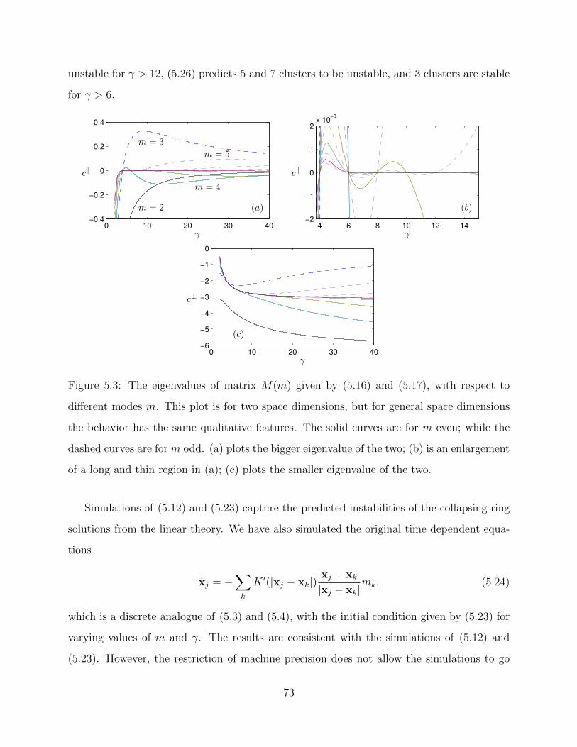
unstable for � > 12, (5.26) predicts 5 and 7 clusters to be unstable, and 3 clusters are stable

for � > 6.

0 10 20 30 40−0.4

−0.2

0

0.2

0.4

(a)m = 2

m = 3

m = 5

m = 4

�

ck

4 6 8 10 12 14−2

−1

0

1

2x 10

−3

(b)

�

ck

0 10 20 30 40−6

−5

−4

−3

−2

−1

0

(c)

�

c?

Figure 5.3: The eigenvalues of matrix M(m) given by (5.16) and (5.17), with respect to

di↵erent modes m. This plot is for two space dimensions, but for general space dimensions

the behavior has the same qualitative features. The solid curves are for m even; while the

dashed curves are for m odd. (a) plots the bigger eigenvalue of the two; (b) is an enlargement

of a long and thin region in (a); (c) plots the smaller eigenvalue of the two.

Simulations of (5.12) and (5.23) capture the predicted instabilities of the collapsing ring

solutions from the linear theory. We have also simulated the original time dependent equa-

tions

xj

= �X

k

K 0(|xj

� xk

|) xj

� xk

|xj

� xk

|mk

, (5.24)

which is a discrete analogue of (5.3) and (5.4), with the initial condition given by (5.23) for

varying values of m and �. The results are consistent with the simulations of (5.12) and

(5.23). However, the restriction of machine precision does not allow the simulations to go

73

too far in time. The simulations are not trustworthy when the collapsing ring approaches

the roundo↵ error.

The stability of all the mode m perturbations of Sd�1 as indicated by Table 5.1 agrees

exactly with the calculation of M(m) given by (5.16) and (5.17) for modes 2 to 10 for

2 < � 20. We more closely investigate the eigenvalues (and hence stability) dependence on

� in Figure 5.3. In Figure 5.3(a) we plot the bigger of the two eigenvalues, which generally

corresponds to tangential perturbations; in Figure 5.3(b) we plot the smaller of the two

eigenvalues, and mainly corresponds to the radial perturbations; and in Figure 5.3(c) we

have enlarged a thin and long region in Figure 5.3(a) that exhibits the oscillating pattern of

the behavior of the bigger eigenvalues with respect to parameter �.

In Figures 5.1 and 5.2, we see cases when Sd�1 is unstable and in each of these examples,

Sd�1 breaks up and collapses to clusters of points. In R2, the most commonly observed long

time attractor is a 3 point cluster that are 3 vertices of an equilateral triangle. In higher

dimensions this behavior continues, i.e., in R3 the generic attractor is a 4 point cluster that

forms the vertices of a tetrahedron. In the next section, we explain why we observe these

attractors by studying the stability of these cluster solutions.

74

5.3 Cluster Stability

5.3.1 Stability of Clusters in R2

By plugging in our specific kernel f defined in (5.13) to (4.3) and (4.4) in Section 4.1, we

arrive at:

c?=

1

m

mX

k

0=1

✓� � �

2(2r sin

⇡k0

m)��2 +

� � 2

2(2r sin

⇡k0

m)��2 cos

2⇡k0

m

◆,

ck=

1

m

mX

k

0=1

✓� � �

2(2r sin

⇡k0

m)��2 � � � 2

2(2r sin

⇡k0

m)��2 cos

2⇡k0

m

◆. (5.25)

8>>>>>>>>>>>>><

>>>>>>>>>>>>>:

A1,1 =1

��2 � �

2(��2)

Pm�1j=0 sin��2 ⇡j

m sin2 ⇡j(l+1)mPm�1

j=0 sin� ⇡jm

, if l 2 {0, . . . , ⇥m2⇤} and l 6= 1;

A1,2 = A2,1 = �12 +

12

Pm�1j=0 sin��2 ⇡j

m sin2 ⇡jlmPm�1

j=0 sin� ⇡jm

, if l 2 {0, . . . , ⇥m2⇤} and l 6= 1;

A2,2 =1

��2 � �

2(��2)

Pm�1j=0 sin��2 ⇡j

m sin2 ⇡j(l�1)mPm�1

j=0 sin� ⇡jm

, if l 2 {0, . . . , ⇥m2⇤} and l 6= 1;

A1,1 =1�2���2 + 2�

��2

Pm�1j=0 sin�+2 ⇡j

mPm�1j=0 sin� ⇡j

m

, if l = 1;

A1,2 = A2,1 = A2,2 = 0, if l = 1.

(5.26)

Equations (5.25) and (5.26) complete the clusters stability in R2 for f . However, since there

is no closed form ofP

m�1k

0=1 sin� ⇡k

0

m

for general � > 2, we cannot evaluate them analytically.

Therefore we numerically investigate equation (5.25) and (5.26) in the next section.

5.3.2 Numerical Simulations of Cluster Stability in R2

Figure 5.4 contains plots of (5.25) for various values of m. From the plot, we see that the

tangential stability of clusters exactly complements the stability of S1 as indicated in Figure

5.3 and Table 5.1. By comparing the stability summary Table 5.1 for S1 with the summary

Table 5.3 for cluster stability we see that, precisely when the ring is unstable (� > 4), there

is at least one cluster that is stable; yet when the ring is stable no cluster is.

Moreover when we look in Figure 5.2 (which is the large � regime) we see the 5 and 7

clusters eventually relax to the equilateral 3 cluster on longer timescales. This is understood

because the 5 and 7 clusters are saddle points which have many decaying directions but

75

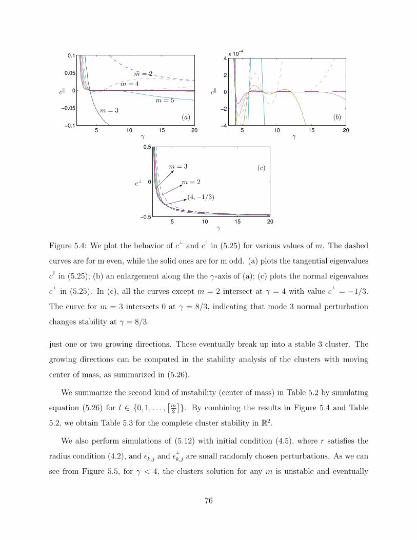
5 10 15 20−0.1

−0.05

0

0.05

0.1

(a)

m = 2

m = 3

m = 5

m = 4

�

ck

5 10 15 20−4

−2

0

2

4x 10

−4

(b)

�

ck

5 10 15 20−0.5

0

0.5

(c)

⇠⇠⇠:(4,�1/3)���*m = 2���✓m = 3

�

c?

Figure 5.4: We plot the behavior of c?and c

kin (5.25) for various values of m. The dashed

curves are for m even, while the solid ones are for m odd. (a) plots the tangential eigenvalues

ckin (5.25); (b) an enlargement along the the �-axis of (a); (c) plots the normal eigenvalues

c?in (5.25). In (c), all the curves except m = 2 intersect at � = 4 with value c

?= �1/3.

The curve for m = 3 intersects 0 at � = 8/3, indicating that mode 3 normal perturbation

changes stability at � = 8/3.

just one or two growing directions. These eventually break up into a stable 3 cluster. The

growing directions can be computed in the stability analysis of the clusters with moving

center of mass, as summarized in (5.26).

We summarize the second kind of instability (center of mass) in Table 5.2 by simulating

equation (5.26) for l 2 {0, 1, . . . , ⇥m2⇤}. By combining the results in Figure 5.4 and Table

5.2, we obtain Table 5.3 for the complete cluster stability in R2.

We also perform simulations of (5.12) with initial condition (4.5), where r satisfies the

radius condition (4.2), and ✏kk,j

and ✏?k,j

are small randomly chosen perturbations. As we can

see from Figure 5.5, for � < 4, the clusters solution for any m is unstable and eventually

76

m = 3 or m = 4 m = 5 m � 6

� 2 (2, 4] stable stable stable

� 2 (4, 6] stable stable unstable

� 2 (6,1) stable unstable unstable

Table 5.2: Stability table for center of mass of clusters, corresponding to the second kind

of instability. It is stable if and only if the eigenvalues of A(l) defined by (5.26) are all

nonpositive.

m = 3 m = 4 or m = 5 m � 6

� 2 (2, 4] unstable unstable unstable

� 2 (4, 6] stable stable unstable

� 2 (6,1) stable unstable unstable

Table 5.3: Stability table for m clusters, combining both kinds of instabilities. It is stable if

and only if conditions 1 and 2 in Theorem 4.2.2 are satisfied.

expands to a circle, but for � > 4, m clusters always deform to 3 clusters, except for some

cases when 4 < � < 6 with m 2 {4, 5} which agrees precisely with Table 5.3.

5.3.3 Stability of Clusters in Rd

We apply Theorem 4.2.2 in Chapter 4 for stability of clusters in a general dimension d. For

our particular f defined by (5.13), we have � = ��, f 0(0) = �, and f 0(�) = �1, so condition

2 of Theorem 4.2.2 reads � � 2 + 2d�1 . Thus, the simplex configuration is stable for � � 4

and unstable for 2 < � < 4.

5.3.4 Numerical Simulations on Simplex Configuration

Theorem 4.2.2 extends the simplex configuration stability in R2 to arbitrary dimensions

which allows us to conclude that for (5.12) and (5.13), the simplex configuration in Rd is

unstable for 2 < � < 4 and stable for � � 4, for d � 2.

77

� 3 5 7 9m

3

4

5

6

(a) ⌧ = 50

� 3 5 7 9m

3

4

5

6

(b) ⌧ = 10000

Figure 5.5: Numerical simulation of the m clusters problem, with m = 3, 4, 5, 6, and

� = 3, 5, 7, and 9, each hole starting with n = 20 particles with fixed-center small random

perturbation. (a) and (b) are the plot of the particles at time ⌧ = 50 and ⌧ = 10000

respectively.

To observe this phenomena we apply a Range Kutta 45 method to (5.12) with n randomly

selected points {Yi 2 Rd, i 2 {1, 2, . . . n}}. After evolving time long enough, the solution

approaches final steady state, we measure the normalized inner product of all pairs of two

points⇢

Yi

|Yi |· Y

i0

|Yi0 |, i 6= i0

�, (5.27)

and we plot both the final steady state and the probability distribution of the normalized

inner products in Figure 5.6.

It is clear from Figure 5.6 that for � = 3 (in the unstable simplex regime), Sd�1 is the

stable steady state solution for (5.12) and (5.13) while for � > 5 (in the stable simplex

regime), a the simplex solution is the attractor. We also can observe that this behavior is

independent of dimension, just as we expect. For � > 5 in Rd, we have

P✓����

Yi

|Yi |· Y

i0

|Yi0 |

+1

d

����⌧ 1

◆⇡ d

d+ 1

and P✓����

Yi

|Yi |· Y

i0

|Yi0 |

� 1

����⌧ 1

◆⇡ 1

d+ 1,

78

−0.50

0.5

−0.50

0.5

−0.5

0

0.5

−1 0 10

0.2

0.4

0.6

0.8

1

−0.20

0.2

−0.20

0.2

−0.2

0

0.2

−1 0 10

0.2

0.4

0.6

0.8

1

−0.50

0.5

−0.50

0.5

−0.5

0

0.5

−1 0 10

0.2

0.4

0.6

0.8

1

−0.20

0.2−0.20

0.2

−0.2

0

0.2

−1 0 10

0.2

0.4

0.6

0.8

1

−0.20

0.2

−0.20

0.2

−0.3−0.2−0.1

00.1

−1 0 10

0.2

0.4

0.6

0.8

1

−0.50

0.5

−0.50

0.5

−0.5

0

0.5

−1 0 10

0.2

0.4

0.6

0.8

1

(A1) (a1) (B1) (b1) (C1) (c1)

(A2) (a2) (B2) (b2) (C2) (c2)

Figure 5.6: Numerical simulation of (5.12) and (5.13) with n = 150 random initial points

in Rd. Capital letters correspond to simulations done for � = 3 and lower case letters

correspond to � = 5. First Row: Figures (A1) and (a1) are the final computed steady states

in d = 3. Similarly for (B1), (b1) in d = 4 though the plots are projected into R3 by taking

the first three coordinates. (C1) and (c1) are for d = 5 and are projections into R3 by also

taking the first three coordinates. Second Row: (A2), (a2), (B2), (b2), (C2), and (c2) are

plots of the corresponding probability distributions of the normalized inner product of any

two points in the final steady state.

indicating that our simulations are close to simplex configurations. We started these simu-

lations with random distributions of particles so these simulations suggest that the simplex

configuration may be the global attractor for any d � 2 and � � 4.

5.4 Appendix of Chapter 5: Proof of Inequality (5.22)

In proving the criteria for linear stability of Sd�1 in Section 5.2.1, the inequality (5.22) is

required. We provide a proof of this inequality here. Let us define the following quantity:

Q(�,m, d) =�(�2 + d� 1)�(�2 + 1)

�(m+ �

2 + d� 1)�(1�m+ �

2 ). (5.28)

79

Then the RHS of equation (5.22) can be written as:

(3� � � d� 1

� + n� 3) + (� � 2)(�1)m+1Q(�,m, d)

+� + 2d� 4

� + d� 3(�1)mQ(� � 2,m, d). (5.29)

The term Q(�,m, d) can be written out as the following:

Q(�,m, d) =⇧m

i=1(�

2 �m+ i)

⇧m

i=1(�

2 + d� 2 + i). (5.30)

Notice that both |�2 � m + 1| and �

2 are less than �

2 + d + m � 2, so that |Q(�,m, d)| < 1

always. Furthermore, if 2 �

2 m then |Q(�,m, d)| 1�+2d�2 and |Q(��2,m, d)| 1

�+2d�4 ;

while �

2 > m� 1 implies 0 < Q(�,m, d) < ��2m+2�+2d�2 .

We can now assert the inequality (5.22) by considering the following three cases for m � 2:

• When 4 � 2m, we have

(5.29) 3� � � d� 1

� + d� 3+

� � 2

� + 2d� 2

+� + 2n� 4

� + n� 3· 1

� + 2d� 4

=4� � � d� 2

� + d� 3� 2d

� + 2d� 2< 0

• When � > 2m, we have

(5.29) <3� � � d� 1

� + d� 3+ (� � 2)

� � 2m+ 2

� + 2d� 2

+� � 2m

� + d� 3.

80

In the case m � 3, we have

(5.29) <� d� 1

� + d� 3� (� � 2)

✓� � 4

� � 2� � � 2m+ 2

� + 2d� 2

◆

� 2m+ d� 3

� + d� 3

� d� 1

� + d� 3� (� � 2)(� � 2m+ 2)(2m+ 2d� 6)

(� � 2m+ 4)(� + 2d� 2)

� 2m+ d� 3

� + d� 3

<0;

while in the case m = 2, we have

(5.29) < � 2d(� � 2)

� + 2d� 2+

2� � 6

� + d� 3

� 2d(� � 2)

� + 2d� 2+

2� + 2d� 4

� + 2d� 2

�2 ((� � 3)(d� 1)� 1)

� + 2d� 2< 0

• When 2 < � < 4, direct calculations show that we always have (�1)m+1Q(�,m, d) < 0

and (�1)mQ(� � 2,m, d) < 0, and it is easy to see that (5.29) < 0 in this case.

The above three cases exhaust all the possibilities, and hence we conclude that the inequality

(5.22) holds for m � 2, d � 2 and � � 2.

81

CHAPTER 6

Conclusion and Future Works

In chapter 2, we derived the generalized Birkho↵-Rott equation to describe sheet-like solu-

tions of 2D active scalar problems with both gradient and divergence free flows. We present

several examples including the classical vortex sheet, superfluids, and swarming models. This

equation is applied in studying the linear wellposedness theory and weakly nonlinear theory

for the ring solutions of the kinematic aggregation model. It is interesting to understand

the stability of other sheet-like solutions, for example, concentric rings solutions. The gen-

eralized Birkho↵-Rott equation exhibits interesting interactions between the gradient and

incompressible components of the kernel. It would be interesting to understand in detail

such an interaction, for example, the relative influence on the curvature blowup time and

the density blowup time for the superfluids example.

In chapters 3 and 4, we derived the linear wellposedness theory for ring solutions and

clusters. This result has already been generalized to 3D and higher dimensions [VUKB].

However, the question of the stability analysis of a general pattern, especially a co-dimension

zero pattern still remains unknown, largely due to the di�culty of writing down the solution

form. It would be highly interesting to see the stability of the nontrivial cases in Figure

3.1. The generalization of the 2D weakly nonlinear analysis to the three dimensions is an

interesting and challenging problem because of the formulation involving spherical harmonics.

However, its solutions have the potential to predict intra-mode bifurcations, which does not

occur in 2D.

In chapters 4 and 5, We constructed a significant portion of the stability picture of the

aggregation equation with a power law interaction kernel as a dynamical system. This allows

82

us to predict when collapsing solutions will maintain spherical symmetry or when solutions

will self organize into more singular simplex configurations. However, the entire story is not

complete. Global and nonlinear stability of solutions are still open problems. Finally, the

cluster problem in arbitrary dimensions with a general (non-simplex) configuration remains

open.

83

References

[AG] C. Anderson and C. Greengard, On vortex methods, SIAM J. Numer. Anal.,22(3):413–440, 1985.

[B] G. Birkho↵, Helmholtz and Taylor Instability Hydrodynamics Instability, Proceed-ings of the Symposium on Appied Mathematics, 13, 55-76, 1962.

[BB] A. L. Bertozzi and J. Brandman, Finite-time blow-up of Linfty-weak solutions of anaggregation equation, Commun. Math. Sci., 8(1): 45-65, 2010.

[BCCVG] E. Ben-Jacob, I. Cohen, A. Czirok, T. Vicsek, and D.L. Gutnick, Chemomodula-tion of cellular movement, collective formation of vortices by swarming bacteria, andcolonial development, Phys. A, 238, 181197, 1997.

[BCL] A. L. Bertozzi, J. A. Carrillo, and T. Laurent, Blow-up in multidimensional ag-gregation equations with mildly singular interaction kernels, Nonlinearity 22: 683,2009.

[BD] M. Burger and M. Di Francesco, Large time behavior of nonlocal aggregation modelswith nonlinear di↵usion, Networks Heterog. Media 3(4): 749-785, 2008.

[BL] A. L. Bertozzi and T. Laurent, Finite-time blow-up of solutions of an aggregationequation in Rn , Commun. Math. Phys., 274(3): 717-735, 2007.

[BL2] A. L. Bertozzi and T. Laurent, The behavior of solutions of multidimensional aggre-gation equations with mildly singular interaction kernels, Chin. Ann. Math. Ser. B,30(5):463–482, 2009.

[BL2] J.L. Burchnall and A. Lakin, The theorems of Saalschutz and Dougall, Quart. J.Math. 2, 161-166, 1950.

[BCL] A. L. Bertozzi, J. A. Carrillo and T. Laurent, Blow-up in multidimensional aggrega-tion equations with mildly singular interaction kernels, Nonlinearity, 22(3):683–710,2009.

[BV] M. Bodnar and J. J. L. Velazquez, An integro-di↵erential equation arising as a limitof individual cell-based models, J. Di↵er. Equations 222(2): 341380, 2006.

[C] P. Constantin, Geometric statistics in turbulence, SIAM Rev., 36(1):73-98, 1994.

[C2] Y. Chuang, Stability and Scalability of 2D Swarming Patterns, (Ph.D. Thesis), 2006.

[CDFLS] J. A. Carillo, M. DiFrancesco, A. Figalli, T. Laurent, and D. Slepcev, Global-in-time weak measure solutions and finite-time aggregation for nonlocal interactionequations, Duke Math. J., 156: 229, 2011.

84

[CDMBC] Y. L. Chuang, M. R. D’Orsogna, D. Marthaler, A. L. Bertozzi, and L. Chayes,State transitions and the continuum limit for a 2D interacting, self-propelled particlesystem, Physica D: Nonlinear Phenomena, 232(1):pp. 33-47,2007.

[CHDB] Y.-L. Chuang, Y. R. Huang, M. R. D’Orsogna, and A. L. Bertozzi, Multi-vehicleflocking: scalability of cooperative control algorithms using pairwise potentials, IEEEInternational Conference on Robotics and Automation, 2292-2299, 2007.

[CK] H. Cohn and A. Kumar, Algorithmic design of self-assembling structures, PNAS,106(24): 95709575, 2009.

[CL] R. E. Caflisch and J. S. Lowengrub, Convergence of the vortex method for vortexsheets, SIAM Journal on Numerical Analysis, 26(5):pp. 1060–1080, 1989.

[CMT] P. Constantin, A. J. Majda and E. Tabak. Formation of strong fronts in the 2Dquasigeostrophic thermal active scalar, Nonlinearity, 7(6):1495–1533, 1994.

[DCBC] M.R. D’Orsogna, Y.L. Chuang, A.L. Bertozzi and L.S. Chayes, Self-propelled Par-ticles wit hSoft-core Interactions: Patterns, Stability and Collapse, Phys Rev Lett.,96(10), 2006.

[DL] F. J. Dyson and A. Lenard, Stability of matter I., Journal of Mathematical Physics,8:423434, 1967.

[DP] Q. Du and P. Zhang, Existence of weak solutions to some vortex density models,SIAM Journal on Mathematical Analysis, 34(6):1279–1299, 2003.

[DVM] R. Daniels, J. Vanderleyden and J. Michiels, Quorum sensing and swarming migra-tion in bacteria, FEMS Microbiology Reviews, 28(3): 261–289, 2004.

[EWG] L. Edelstein-Keshet, J. Watmough and D. Grurunbau, Do travelling band solu-tions describe cohesive swarms? an investigation for migratory locusts, Journal ofMathematical Biology, 36(6): 515549, 1998.

[HLK] T. Y. Hou, J. Lowengrub and R. Krasny, Convergence of a point vortex method forvortex sheets, SIAM Journal on Numerical Analysis, 28(2):pp. 308–320, 1991.

[HB] Y. Huang and A. L. Bertozzi, Self-similar blowup solutions to an aggregation equa-tion in Rn, SIAM Journal on Applied Mathematics, 70(7):2582–2603, 2010.

[HB2] Y. Huang and A. L. Bertozzi, Asymptotics of blowup solutions for the aggregationequation, DCDS, 17(4):1309–1331, 2012.

[HKM] D. Helbing, J. Keltsch and P. Molnr Modelling the Evolution of Human Trail Sys-tems, Nature, 388: 47-50, 1997.

[KHP] T. Kolokolnikov, Y. Huang and M. Pavlovskia, Singular patterns for an aggregationmodel with a confining potential, Physica D: Nonlinear Phenomena, 2012.

85

[KSUB] T. Kolokolnikov, H. Sun, D. Uminsky and A. L. Bertozzi, Stability of ring patternsarising from two-dimensional particle interactions, Phys. Rev. E, 84(1), 2011.

[K] R. Krasny, Desingularization of periodic vortex sheet roll-up, J. Comput. Phys.,65(2):292–313, 1986.

[K2] R. Krasny, Computation of vortex sheet roll-up in the Tre�tz plane, J. Fluid Mech.,184:123–155, 1987.

[KS] E. F. Keller and L. A. Segel, Initiation of slime mold aggregation viewed as aninstability, J. Theor. Biol., 26:399–415, 1970.

[L] A. Leonard, Vortex methods for flow simulation, J. Comput. Phys., 37(3):289–335,1980.

[L2] T. Laurent, Local and global existence for an aggregation equation, Commun.Partial Di↵er. Equ., 32(12): 1941-1964, 2007.

[LLE] R. Lukeman, Y. X. Li, L. Edelstein-Keshet, How do ducks line up in rows: inferringindividual rules from collective behaviour, PNAS, 107(28): 12576-12580, 2010.

[LRC] H. Levine, W. J. Rappel, and I. Cohen, Self-organization in systems of self-propelledparticles, Phys. Rev. E, 63(1), 2000;

[MB] A. J. Majda and A. L. Bertozzi, Vorticity and Incompressible Flow, CambridgeUniversity Press, 2002.

[MZ] N. Masmoudi and P. Zhang. Global solutions to vortex density equations arisingfrom sup-conductivity, Ann. Inst. H. Poincare Anal. Non Lineaire, 22(4):441–458,2005.

[MZDT] N. Mate, A. Zsuzsa, B. Dora and V. Tams, Hierarchical group dynamics in pigeonflocks Nature, 464, 890–893, 2010.

[O] L. Onsager, Electrostatic interaction of molecules, Journal of Mathematical Physics,43: 189196, 1939.

[OMB] A. Ordemann, F. Moss, and G. Balazsi, Motions of Daphnia in a light field: Randomwalks with a zooplankton, Nova Acta Leopoldina, 88: 87103, 2003.

[P] E. G. Puckett, A study of the vortex sheet method and its rate of convergence, SIAMJ. Sci. Stat. Comput., 10: 298-327, 1989.

[PE] J.K. Parrish and L. Edelstein-Keshet, Complexity, pattern, and evolutionary trade-o↵s in animal aggregation, Science, 284: 99101, 1999.

[PVG] J. Parrish, S. V. Viscido, and D. Grunbaum, Self-organized fish schools: an exami-nation of emergent properties, Biology Bulletin, 202:296305, 2002.

86

[R] D. Ruelle, Statistical Mechanics, Rigorous Results, New York: W.A. Benjamin,1969.

[R2] W. L. Romey, Individual di↵erences make a di↵erence in the trajectories of simulatedschools of fish, Ecological Modelling, 92(1): 65-77, 1996.

[RB] H. Reuter and B. Breckling, Selforganization of fish schools: an object- orientedmodel, Ecological Modelling, 75/76:147159, 1994.

[RNSL] W.J. Rappel, A. Nicol, A. Sarkissian, and H. Levine, Self-organized vortex state intwo-dimensional Dictyostelium dynamics, Phys. Rev. Lett., 83: 12471250, 1999.

[RST] M. C. Rechtsman, F. H. Stillinger, and S. Torquato, Optimized Interactions forTargeted Self-Assembly: Application to a Honeycomb Lattice, Phys. Rev. Lett.,95(22): 2005.

[RST2] M. C. Rechtsman, F. H. Stillinger, and S. Torquato, Synthetic diamond and wurtzitestructures self-assemble with isotropic pair interactions, Phys. Rev. E, 75(3): 2007.

[S] M. J. Shelley, A study of singularity formation in vortex-sheet motion by a spectrallyaccurate vortex method, Journal of Fluid Mechanics, 244:493-526, 1992.

[S2] G. Szego, Orthogonal polynomials, American Mathematical Society, 1975

[S3] L.J. Slater, Generalized Hypergeometric Functions, Cambridge University Press,1966.

[S4] T. C. Schneirla, Army Ants: A Study in Social Organization, Freeman & CompanyW. H., 1971.

[SB] P. Sa↵man and G. Baker, Vortex Interactions, Ann. Rev. Fluid Mech. , 11, 95-122,1979.

[SSBF] C. Sulem, P.-L. Sulem, C. Bardos and U. Frisch, Finite time analyticity for the two-and three-dimensional Kelvin-Helmholtz instability, Comm. Math. Phys., 80(4):485–516, 1981.

[SUB] H. Sun, D. Uminsky and A. L. Bertozzi, A Generalized Birkho↵Rott Equation forTwo-dimensional Active Scalar Problems, SIAM J. Appl. Math., 72:382-404, 2012.

[SUB2] H. Sun, D. Uminsky and A. L. Bertozzi, Stability and clustering of self-similarsolutions of aggregation equations, J. Math. Phys. Special Issue on IncompressibleFluids, Turbulence and Mixing, 53(11), 2012.

[TB] C. M. Topaz and A. L. Bertozzi, Swarming patterns in a two-dimensional kinematicmodel for biological groups, SIAM Journal on Applied Mathematics, 65(1):152–174,2004.

87

[TT] J. Toner and Y. Tu, Long-range order in a two-dimensional dynamical xy model:how birds fly together, Phys. Rev. Lett., 75(23): 43264329, 1995.

[VB] J. H. von Brecht and A. L. Bertozzi Well-posedness theory for aggregtion sheets,Communications in Mathematical Physics, 2012.

[VBDFFVM] N. Verstraeten, K. Braeken, B. Debkumari, M. Fauvart, J. Fransaer, J. Ver-mant and J. Michiels, Living on a surface: swarming and biofilm formation, Trendsin Microbiology, 16(10):496–506, 2008.

[VU] J. H. von Brecht and D. Uminsky, On Soccer Balls and Linearized Inverse StatisticalMechanics, Journal of Nonlinear Science, 22(6):935–959, 2012.

[VUKB] J. H. von Brecht, D. Uminsky, T. Kolokonikov and A. L. Bertozzi, Predictingpattern formation in particle interactions, M3AS, 22(supp01), 1140002, 2012.

[W] E. Weinan, Dynamics of vortex liquids in Ginzburg-Landau theories with applica-tions to superconductivity, Phys. Rev. B, 50(2):1126–1135, 1994.

[Y] V. I. Yudovich. Non-stationary flow of an ideal incompressible liquid, USSR Com-putational Mathematics and Mathematical Physics, 3(6):14071456, 1963.

88