Singular value decomposition

CSE 250B

Singular value decomposition (SVD)For symmetric matrices, e.g. covariance matrices, we’ve seen:

• Results about existence of eigenvalues and eigenvectors

• The fact that the eigenvectors form an alternative basis

• The resulting spectral decomposition, used in PCA

What about arbitrary matrices M ∈ Rp×q?

Any p× q matrix (say p ≤ q) has singular value decomposition:

M =

x xu1 · · · upy y

︸ ︷︷ ︸

p × p matrix U

σ1 · · · 0...

. . ....

0 · · · σp

︸ ︷︷ ︸

p × p matrix Λ

←−−−− v1 −−−−→...

←−−−− vp −−−−→

︸ ︷︷ ︸

p × q matrix VT

• u1, . . . , up are orthonormal vectors in Rp

• v1, . . . , vp are orthonormal vectors in Rq

• σ1 ≥ σ2 ≥ · · · ≥ σp are singular values

Matrix approximationWe can factor any p × q matrix as M = UW T :

M =

x xu1 · · · upy y

σ1 · · · 0

.... . .

...0 · · · σp

←−−−− v1 −−−−→

...←−−−− vp −−−−→

=

x xu1 · · · upy y

︸ ︷︷ ︸

p × p matrix U

←−−−− σ1v1 −−−−→...

←−−−− σpvp −−−−→

︸ ︷︷ ︸

p × q matrix WT

Concise approximation to M: for k < p, take

M̂ =

x xu1 · · · uky y

︸ ︷︷ ︸

p×k

←−−−− σ1v1 −−−−→...

←−−−− σkvk −−−−→

︸ ︷︷ ︸

k×q

Low-rank approximation of a matrix

Suppose we want to approximate a matrix M by a simpler matrixM̂. What is a suitable notion of “simple”?

• Let’s say M and M̂ are p × q, where p ≤ q.

• Treat each row of M̂ as a data point in Rq.

• One type of simplicity: data is in a low-dimensional subspace.

• If rows lie in k-dimensional subspace, say M̂ has rank k.

The rank of a matrix is the number of linearly independent rows.

Low-rank approximation: given M ∈ Rp×q and an integer k , findthe matrix M̂ ∈ Rp×q that is the best rank-k approximation to M.

That is, find M̂ so that

• M̂ has rank ≤ k

• The approximation error∑

i ,j(Mij − M̂ij)2 is minimized.

SVD gives us the best rank-k approximation M̂.

Example: topic modeling

Blei (2012):

78 COMMUNICATIONS OF THE ACM | APRIL 2012 | VOL. 55 | NO. 4

review articles

time. (See, for example, Figure 3 for topics found by analyzing the Yale Law Journal.) Topic modeling algorithms do not require any prior annotations or labeling of the documents—the topics emerge from the analysis of the origi-nal texts. Topic modeling enables us to organize and summarize electronic archives at a scale that would be impos-sible by human annotation.

Latent Dirichlet AllocationWe first describe the basic ideas behind latent Dirichlet allocation (LDA), which is the simplest topic model.8 The intu-ition behind LDA is that documents exhibit multiple topics. For example, consider the article in Figure 1. This article, entitled “Seeking Life’s Bare (Genetic) Necessities,” is about using data analysis to determine the number of genes an organism needs to survive (in an evolutionary sense).

By hand, we have highlighted differ-ent words that are used in the article. Words about data analysis, such as “computer” and “prediction,” are high-lighted in blue; words about evolutionary biology, such as “life” and “organism,” are highlighted in pink; words about genetics, such as “sequenced” and

“genes,” are highlighted in yellow. If we took the time to highlight every word in the article, you would see that this arti-cle blends genetics, data analysis, and evolutionary biology in different pro-portions. (We exclude words, such as “and” “but” or “if,” which contain little topical content.) Furthermore, know-ing that this article blends those topics would help you situate it in a collection of scientific articles.

LDA is a statistical model of docu-ment collections that tries to capture this intuition. It is most easily described by its generative process, the imaginary random process by which the model assumes the documents arose. (The interpretation of LDA as a probabilistic model is fleshed out later.)

We formally define a topic to be a distribution over a fixed vocabulary. For example, the genetics topic has words about genetics with high probability and the evolutionary biology topic has words about evolutionary biology with high probability. We assume that these topics are specified before any data has been generated.a Now for each

a Technically, the model assumes that the top-ics are generated first, before the documents.

document in the collection, we gener-ate the words in a two-stage process.

! Randomly choose a distribution over topics.

! For each word in the documenta. Randomly choose a topic from

the distribution over topics in step #1.

b. Randomly choose a word from the corresponding distribution over the vocabulary.

This statistical model reflects the intuition that documents exhibit mul-tiple topics. Each document exhib-its the topics in different proportion (step #1); each word in each docu-ment is drawn from one of the topics (step #2b), where the selected topic is chosen from the per-document distri-bution over topics (step #2a).b

In the example article, the distri-bution over topics would place prob-ability on genetics, data analysis, and

b We should explain the mysterious name, “latent Dirichlet allocation.” The distribution that is used to draw the per-document topic distribu-tions in step #1 (the cartoon histogram in Figure 1) is called a Dirichlet distribution. In the genera-tive process for LDA, the result of the Dirichlet is used to allocate the words of the document to different topics. Why latent? Keep reading.

Figure 1. The intuitions behind latent Dirichlet allocation. We assume that some number of “topics,” which are distributions over words, exist for the whole collection (far left). Each document is assumed to be generated as follows. First choose a distribution over the topics (the histogram at right); then, for each word, choose a topic assignment (the colored coins) and choose the word from the corresponding topic. The topics and topic assignments in this figure are illustrative—they are not fit from real data. See Figure 2 for topics fit from data.

. , ,

. , ,

. . .

genednagenetic

lifeevolveorganism

brainneuronnerve

datanumbercomputer. , ,

Topics DocumentsTopic proportions and

assignments

0.040.020.01

0.040.020.01

0.020.010.01

0.020.020.01

datanumbercomputer. , ,

0.020.020.01

Latent semantic indexing (LSI)

Given a large corpus of n documents:

• Fix a vocabulary, say of V words.

• Bag-of-words representation for documents: each documentbecomes a vector of length V , with one coordinate per word.

• The corpus is an n × V matrix, one row per document.

cat

dog

hous

ebo

atga

rden

· · ·Doc 1 4 1 1 0 2Doc 2 0 0 3 1 0Doc 3 0 1 3 0 0

...

Let’s find a concise approximation to this matrix M.

Latent semantic indexing, cont’d

SVD yields an approximation to M: for small k ,←−− doc 1 −−→←−− doc 2 −−→←−− doc 3 −−→

...←−− doc n −−→

︸ ︷︷ ︸

n × V matrix M

≈

←−− θ1 −−→←−− θ2 −−→←−− θ3 −−→

...←−− θn −−→

︸ ︷︷ ︸

n × k matrix Θ

←−−−− Ψ1 −−−−→...

←−−−− Ψk −−−−→

︸ ︷︷ ︸

k × V matrix Ψ

Think of this as a topic model with k topics.

• Ψj is a vector of length V describing topic j : coefficient Ψjw

is large if word w appears often in that topic.

• Each document is a combination of topics: θij is the weight oftopic j in document i .

Document i originally represented by ith row of M, a vector in RV .Instead use θi ∈ Rk , more concise “semantic” representation.

Example: Collaborative filtering

Details and images from Koren, Bell, Volinksy (2009).

Recommender systems: matching customers with products.

• Given: data on prior purchases/interests of users

• Recommend: further products of interest

Prototypical example: Netflix.

A successful approach: collaborative filtering.

• Model dependencies between different products, and betweendifferent users.

• Can give reasonable recommendations to a relatively new user.

Two strategies for collaborative filtering:

• Neighborhood methods

• Latent factor methods

Neighborhood methods

43AUGUST 2009

well-defined dimensions such as depth of character de-velopment or quirkiness; or completely uninterpretable dimensions. For users, each factor measures how much the user likes movies that score high on the correspond-ing movie factor.

Figure 2 illustrates this idea for a simplified example in two dimensions. Consider two hypothetical dimen-sions characterized as female- versus male-oriented and serious versus escapist. The figure shows where several well-known movies and a few fictitious users might fall on these two dimensions. For this model, a user’s predicted rating for a movie, relative to the movie’s average rating, would equal the dot product of the movie’s and user’s lo-cations on the graph. For example, we would expect Gus to love Dumb and Dumber, to hate The Color Purple, and to rate Braveheart about average. Note that some mov-ies—for example, Ocean’s 11—and users—for example, Dave—would be characterized as fairly neutral on these two dimensions.

MATRIX FACTORIZATION METHODSSome of the most successful realizations of latent factor

models are based on matrix factorization. In its basic form, matrix factorization characterizes both items and users by vectors of factors inferred from item rating patterns. High correspondence between item and user factors leads to a

each song in the Music Genome Project based on hundreds of distinct musical characteristics. These attributes, or genes, capture not only a song’s musical identity but also many significant qualities that are relevant to understanding listeners’ musi-cal preferences.

An alternative to content filtering relies only on past user behavior—for example, previous transactions or product ratings—without requiring the creation of explicit profiles. This approach is known as col-laborative filtering, a term coined by the developers of Tapestry, the first recom-mender system.1 Collaborative filtering analyzes relationships between users and interdependencies among products to identify new user-item associations.

A major appeal of collaborative fil-tering is that it is domain free, yet it can address data aspects that are often elusive and difficult to profile using content filter-ing. While generally more accurate than content-based techniques, collaborative filtering suffers from what is called the cold start problem, due to its inability to ad-dress the system’s new products and users. In this aspect, content filtering is superior.

The two primary areas of collaborative filtering are the neighborhood methods and latent factor models. Neighbor-hood methods are centered on computing the relationships between items or, alternatively, between users. The item-oriented approach evaluates a user’s preference for an item based on ratings of “neighboring” items by the same user. A product’s neighbors are other products that tend to get similar ratings when rated by the same user. For example, consider the movie Saving Private Ryan. Its neighbors might include war movies, Spielberg movies, and Tom Hanks movies, among others. To predict a par-ticular user’s rating for Saving Private Ryan, we would look for the movie’s nearest neighbors that this user actually rated. As Figure 1 illustrates, the user-oriented approach identifies like-minded users who can complement each other’s ratings.

Latent factor models are an alternative approach that tries to explain the ratings by characterizing both items and users on, say, 20 to 100 factors inferred from the ratings patterns. In a sense, such factors comprise a computerized alternative to the aforementioned human-created song genes. For movies, the discovered factors might measure obvious dimensions such as comedy versus drama, amount of action, or orientation to children; less

Joe

#2

#3

#1

#4

Figure 1. The user-oriented neighborhood method. Joe likes the three movies on the left. To make a prediction for him, the system finds similar users who also liked those movies, and then determines which other movies they liked. In this case, all three liked Saving Private Ryan, so that is the first recommendation. Two of them liked Dune, so that is next, and so on.

Latent factor methodsCOVER FE ATURE

COMPUTER 44

vector qi R f, and each user u is associ-ated with a vector pu R f. For a given item i, the elements of qi measure the extent to which the item possesses those factors, positive or negative. For a given user u, the elements of pu measure the extent of interest the user has in items that are high on the corresponding factors, again, posi-tive or negative. The resulting dot product, qi

T pu, captures the interaction between user u and item i—the user’s overall interest in the item’s characteristics. This approximates user u’s rating of item i, which is denoted by rui, leading to the estimate

r̂ui

= qiT pu. (1)

The major challenge is computing the map-ping of each item and user to factor vectors qi, pu R f. After the recommender system completes this mapping, it can easily esti-mate the rating a user will give to any item by using Equation 1.

Such a model is closely related to singular value decom-position (SVD), a well-established technique for identifying latent semantic factors in information retrieval. Applying SVD in the collaborative filtering domain requires factoring the user-item rating matrix. This often raises difficulties due to the high portion of missing values caused by sparse-ness in the user-item ratings matrix. Conventional SVD is undefined when knowledge about the matrix is incom-plete. Moreover, carelessly addressing only the relatively few known entries is highly prone to overfitting.

Earlier systems relied on imputation to fill in missing ratings and make the rating matrix dense.2 However, im-putation can be very expensive as it significantly increases the amount of data. In addition, inaccurate imputation might distort the data considerably. Hence, more recent works3-6 suggested modeling directly the observed rat-ings only, while avoiding overfitting through a regularized model. To learn the factor vectors (pu and qi), the system minimizes the regularized squared error on the set of known ratings:

min* *,q p ( , )u i

(rui qiTpu)

2 + (|| qi ||2 + || pu ||

2) (2)

Here, is the set of the (u,i) pairs for which rui is known (the training set).

The system learns the model by fitting the previously observed ratings. However, the goal is to generalize those previous ratings in a way that predicts future, unknown ratings. Thus, the system should avoid overfitting the observed data by regularizing the learned parameters, whose magnitudes are penalized. The constant controls

recommendation. These methods have become popular in recent years by combining good scalability with predictive accuracy. In addition, they offer much flexibility for model-ing various real-life situations.

Recommender systems rely on different types of input data, which are often placed in a matrix with one dimension representing users and the other dimension representing items of interest. The most convenient data is high-quality explicit feedback, which includes explicit input by users regarding their interest in products. For example, Netflix collects star ratings for movies, and TiVo users indicate their preferences for TV shows by pressing thumbs-up and thumbs-down buttons. We refer to explicit user feedback as ratings. Usually, explicit feedback com-prises a sparse matrix, since any single user is likely to have rated only a small percentage of possible items.

One strength of matrix factorization is that it allows incorporation of additional information. When explicit feedback is not available, recommender systems can infer user preferences using implicit feedback, which indirectly reflects opinion by observing user behavior including pur-chase history, browsing history, search patterns, or even mouse movements. Implicit feedback usually denotes the presence or absence of an event, so it is typically repre-sented by a densely filled matrix.

A BASIC MATRIX FACTORIZATION MODEL Matrix factorization models map both users and items

to a joint latent factor space of dimensionality f, such that user-item interactions are modeled as inner products in that space. Accordingly, each item i is associated with a

Gearedtowardmales

Serious

Escapist

The PrincessDiaries

Braveheart

Lethal Weapon

IndependenceDay

Ocean’s 11Sense andSensibility

Gus

Dave

Gearedtoward

females

Amadeus

The Lion King Dumb andDumber

The Color Purple

Figure 2. A simplified illustration of the latent factor approach, which characterizes both users and movies using two axes—male versus female and serious versus escapist.

The matrix factorization approach

User ratings are assembled in a large matrix M:

Star

War

sM

atrix

Cas

abla

nca

Cam

elot

God

fath

er

· · ·User 1 5 5 2 0 0User 2 0 0 3 4 5User 3 0 0 5 0 0

...

• Not rated = 0, otherwise scores 1-5.

• For n users and p movies, this has size n × p.

• Most entries unavailable: we’d like to predict these.

Idea: Use low-rank approximation of M to fill in missing entries.

User and movie factors

Best rank-k approximation is of the form M ≈ UW T :←−− user 1 −−→←−− user 2 −−→←−− user 3 −−→

...←−− user n −−→

︸ ︷︷ ︸

n × p matrix M

≈

←−− u1 −−→←−− u2 −−→←−− u3 −−→

...←−− un −−→

︸ ︷︷ ︸

n × k matrix U

x x xw1 w2 · · · wpy y y

︸ ︷︷ ︸

k × p matrix WT

Thus user i ’s rating of movie j is approximated as

Mij ≈ ui · wj

Users and movies in same “latent” k-dimensional space:

• Represent ith user by ui ∈ Rk

• Represent jth movie by wj ∈ Rk

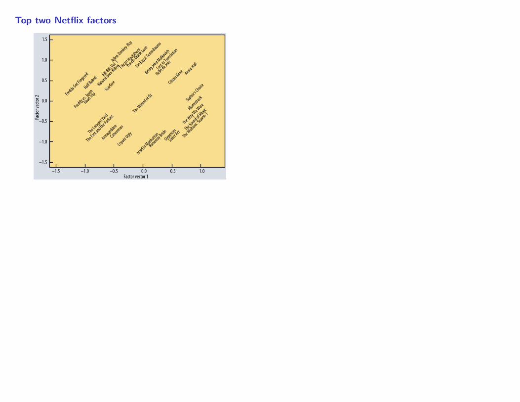
Top two Netflix factors

47AUGUST 2009

Our winning entries consist of more than 100 differ-ent predictor sets, the majority of which are factorization models using some variants of the methods described here. Our discussions with other top teams and postings on the public contest forum indicate that these are the most popu-lar and successful methods for predicting ratings.

Factorizing the Netflix user-movie matrix allows us to discover the most descriptive dimensions for predict-ing movie preferences. We can identify the first few most important dimensions from a matrix decomposition and explore the movies’ location in this new space. Figure 3 shows the first two factors from the Netflix data matrix factorization. Movies are placed according to their factor vectors. Someone familiar with the movies shown can see clear meaning in the latent factors. The first factor vector (x-axis) has on one side lowbrow comedies and horror movies, aimed at a male or adolescent audience (Half Baked, Freddy vs. Jason), while the other side contains drama or comedy with serious undertones and strong female leads (Sophie’s Choice, Moonstruck). The second factorization axis (y-axis) has independent, critically acclaimed, quirky films (Punch-Drunk Love, I Heart Huckabees) on the top, and on the bottom, mainstream formulaic films (Armaged-don, Runaway Bride). There are interesting intersections between these boundaries: On the top left corner, where indie meets lowbrow, are Kill Bill and Natural Born Kill-ers, both arty movies that play off violent themes. On the bottom right, where the serious female-driven movies meet

preferences might cause a one-time event; however, a recurring event is more likely to reflect user opinion.

The matrix factorization model can readily accept varying confidence levels, which let it give less weight to less meaningful observations. If con-fidence in observing rui is denoted as cui, then the model enhances the cost function (Equation 5) to account for confidence as follows:

min* * *, ,p q b

( , )u i

cui(rui µ bu bi

puTqi)

2 + (|| pu ||2 + || qi ||

2 + bu

2 + bi2) (8)

For information on a real-life ap-plication involving such schemes, refer to “Collaborative Filtering for Implicit Feedback Datasets.”10

NETFLIX PRIZE COMPETITION

In 2006, the online DVD rental company Netflix announced a con-test to improve the state of its recommender system.12 To enable this, the company released a training set of more than 100 million ratings spanning about 500,000 anony-mous customers and their ratings on more than 17,000 movies, each movie being rated on a scale of 1 to 5 stars. Participating teams submit predicted ratings for a test set of approximately 3 million ratings, and Netflix calculates a root-mean -square error (RMSE) based on the held-out truth. The first team that can improve on the Netflix algo-rithm’s RMSE performance by 10 percent or more wins a $1 million prize. If no team reaches the 10 percent goal, Netflix gives a $50,000 Progress Prize to the team in first place after each year of the competition.

The contest created a buzz within the collaborative fil-tering field. Until this point, the only publicly available data for collaborative filtering research was orders of magni-tude smaller. The release of this data and the competition’s allure spurred a burst of energy and activity. According to the contest website (www.netflixprize.com), more than 48,000 teams from 182 different countries have down-loaded the data.

Our team’s entry, originally called BellKor, took over the top spot in the competition in the summer of 2007, and won the 2007 Progress Prize with the best score at the time: 8.43 percent better than Netflix. Later, we aligned with team Big Chaos to win the 2008 Progress Prize with a score of 9.46 percent. At the time of this writing, we are still in first place, inching toward the 10 percent landmark.

–1.5 –1.0 –0.5 0.0 0.5 1.0

–1.5

–1.0

–0.5

0.0

0.5

1.0

1.5

Factor vector 1

Facto

r vec

tor 2

Freddy Got Fingered

Freddy vs. Jason

Half Baked

Road Trip

The Sound of Music

Sophie’s Choice

Moonstruck

Maid in Manhattan

The Way We Were

Runaway Bride

Coyote Ugly

The Royal Tenenbaums

Punch-Drunk Love

I Heart Huckabees

Armageddon

Citizen Kane

The Waltons: Season 1

Stepmom

Julien Donkey-Boy

Sister Act

The Fast and the Furious

The Wizard of Oz

Kill Bill:

Vol. 1

ScarfaceNatural Born Killers

Annie Hall

Belle de JourLost i

n Translation

The Longest Yard

Being John Malkovich

Catwoman

Figure 3. The first two vectors from a matrix decomposition of the Netflix Prize data. Selected movies are placed at the appropriate spot based on their factor vectors in two dimensions. The plot reveals distinct genres, including clusters of movies with strong female leads, fraternity humor, and quirky independent films.