Embed Size (px)
Citation preview
Skin Strain Field Analysis of the Human Ankle Joint
Sara Sofia Pereira Marreiros
Dissertação para obtenção do Grau de Mestre em
Engenharia Biomédica
Júri
Presidente: Professor Doutor Hélder Carriço Rodrigues
Orientadores: Professor Doutor Jorge Manuel Mateus Martins
Professor Doutor Miguel Pedro Tavares da Silva
Professor Doutor João Nuno Marques Parracho Guerra da Costa
Vogais: Professor Doutor João Orlando Marques Gameiro Folgado
Professor Doutor Mamede de Carvalho
Novembro 2010
FACULDADE DE MEDICINA Universidade de Lisboa


I
Acknowledgments
I thank to:
Prof. Miguel Silva
Prof. Jorge Martins
Prof. João Folgado
Diana Lopes
Marta Faria
Ana Coito
Pedro Custódio
Sérgio Gonçalves
Paulo Melo
Daniel Lopes
Miguel Guerreiro
Antónia and Fernando Marreiros
And to all of my friends and colleges from IST

II
III
Resumo
As Linhas de Não Extensão (LoNE do inglês lines of non-extension) representam as direcções na
pele onde, durante o movimento humano, esta não deforma. O uso das LoNE no projecto de uma
ortótese que irá actuar como uma segunda pele é uma nova abordagem para a correcção do pé
pendente.
O principal objectivo deste trabalho é, obter o mapa de deformações da pele do tornozelo e do
pé, para os movimentos mais amplos do tornozelo, e encontrar as direcções das LoNE nesta mesma
região. A recolha dos dados relativos à deformação da pele foi feita recorrendo a um sistema de
quatro câmaras de infravermelhos que calcula as posições espaciais de marcadores reflectores
colocados sobre a pele. O cálculo do tensor das deformações da pele para os movimentos
analisados, flexão plantar e dorsiflexão, foi realizado por um software de elementos finitos. Foi
desenvolvido um programa computacional que utiliza os cálculos realizados pelo software para
calcular as magnitudes e as direcções das tensões principais na pele. Este mesmo programa utiliza
os resultados anteriores para calcular as direcções de deformação mínima na pele. Estes cálculos
foram realizados para os movimentos mais amplos e as direcções encontradas foram consideradas
válidas para movimentos com amplitudes intermédias. Finalmente as LoNE, encontradas a partir dos
resultados obtidos, foram desenhadas. Obtiveram-se sete conjuntos de linhas de não extensão na
região analisada.
Palavras-Chave: Linhas de Não Extensão, Segunda Pele, Pé Pendente, Campo de Tensões na Pele,
Movimento do Tornozelo, Ortoteses do Pé e do Tornozelo.

IV

V
Abstract
The Lines of Non-Extension (LoNE) represent the skin’s directions where, during human motion, the
skin doesn’t deform. The use of the LoNE in the design of an orthosis that will act like a second skin is
a new approach for the drop-foot pathology correction.
The main purpose of this work is to obtain the strain field maps of the ankle and foot’s skin, for
the ankle’s large movements, and find the directions of the LoNE in the same region. The acquisition
of the skin’s deformations data were performed with a system of four infrared cameras that calculate
the spatial position of reflective markers placed on the skin. The skin’s strain tensor calculus from the
analyzed movements, plantar flexion and dorsiflexion, were performed by a finite element software. A
computational program was developed that uses the calculus performed by this software and
calculates the magnitude and direction of the principal skin strains. The developed program uses the
previous results to calculate the directions of minimum skin strain. All the directions were obtained for
the larger movements and they were considered valid for the movements with intermediate
amplitudes. Finally, the LoNE found based in the obtained results were drawn and seven sets of lines
on non-extension were obtained in the analyzed skin’s region.
Keywords: Lines of Non-Extension, Second Skin, Drop-foot, Skin’s Strain Field, Ankle Motion, Ankle-
Foot Orthoses.

VI

VII
Table of Contents
1. Introduction .............................................................................................................................................. 1
1.1 Motivation ................................................................................................................................ 1
1.2 Objectives ................................................................................................................................ 2
1.3 Literature Review ..................................................................................................................... 2
1.4 Contributions............................................................................................................................ 3
1.5 Thesis Organization ................................................................................................................. 4
2. Human Motion ......................................................................................................................................... 5
2.1 Lower limb’s anatomy .............................................................................................................. 5
2.2 Reference Terminology of the human body ............................................................................ 6
2.3 Terminology of the Joint’s Movements .................................................................................... 8
2.4 Human gait cycle ..................................................................................................................... 9
2.5 Ankle Joint ............................................................................................................................. 11
2.5.1 Ankle movements during Gait Cycle ..............................................................................11
2.5.2 Ankle Muscle Control ......................................................................................................12
Dorsiflexors ................................................................................................................................. 12
Plantar Flexors ............................................................................................................................ 13
2.5.3 Ankle Pathologies ...........................................................................................................13
Drop-foot ..................................................................................................................................... 13
3. Ankle-Foot Orthoses (AFO) ................................................................................................................... 17
3.1 Ankle-Foot Orthoses .............................................................................................................. 17
3.1.1 Rigid Ankle Foot Orthoses (AFOs) .................................................................................17
3.1.2 Articulated Ankle-Foot Orthoses .....................................................................................17
3.1.3 Dynamic Ankle-Foot Orthoses (DAFOs) ........................................................................18
3.1.4 Active Ankle-Foot Orthoses ............................................................................................19
4. Human Skin ........................................................................................................................................... 21
4.1 Histology of the Human Skin ................................................................................................. 21
4.2 Biomechanical Properties of the Skin .................................................................................... 22
4.3 Langer’s Lines ....................................................................................................................... 24
4.4 Lines of Non-Extension (LoNE) ............................................................................................. 25
5. Strain Field Analysis .............................................................................................................................. 29

VIII
5.1 Kinematics of Deformation .................................................................................................... 29
5.2 Mohr’s Circle .......................................................................................................................... 31
6. Laboratory Procedure and Developed Program.................................................................................... 33
6.1 Acquisition system ................................................................................................................. 33
6.2 Marker Placement ................................................................................................................. 34
6.3 Analyzed Movements ............................................................................................................ 35
6.4 Data Treatment and Analysis ................................................................................................ 36
6.4.1 Data acquisition using the Qualisys Track Manager (QTM) software ............................36
6.4.2 Data organization and pre processing in MATLAB ........................................................36
6.4.3 Calculus of the strain tensor using ABAQUS and FORTRAN ........................................38
6.4.4 Principal Strain Directions and Lines of Non-Extension (LoNE) ....................................39
7. Results and Discussion ......................................................................................................................... 43
7.1 Skin’s Strain Field .................................................................................................................. 45
7.2 Directions of Minimum Skin Stretch ...................................................................................... 48
7.3 Lines of Non-Extension ......................................................................................................... 54
7.4 Comparison of results with previous works ........................................................................... 59
8. Conclusions and Future Developments ................................................................................................ 61
8.1 Conclusions ........................................................................................................................... 61
8.2 Future Developments ............................................................................................................ 63
References ................................................................................................................................................. 65
Appendix A ................................................................................................................................................. 69
Appendix B ................................................................................................................................................. 71
IX
List of Figures
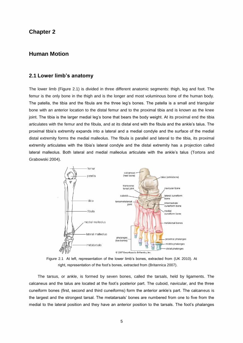
Figure 2.1 At left, representation of the lower limb’s bones, extracted from (UK 2010). At right,
representation of the foot’s bones, extracted from (Britannica 2007). .................................................... 5
Figure 2.2 Representation of the foot’s arches, extracted from (Fitness 2009) ...................................... 6
Figure 2.3 Representation of anatomical reference position and the three anatomical reference planes:
transverse, frontal and sagittal planes (Vaughan, Davis et al. 1992). ..................................................... 7
Figure 2.4 Representation of the ankle joint movements on a parallel plane to the sagittal plane:
dorsiflexion and plantar flexion (Hall 1991). ............................................................................................ 8
Figure 2.5 Representation of the ankle joint movements in the frontal plane: eversion and inversion
(Hall 1991). .............................................................................................................................................. 8
Figure 2.6 Representation of the normal gait cycle in a eight years old boy (Vaughan, Davis et al.
1992). ..................................................................................................................................................... 10
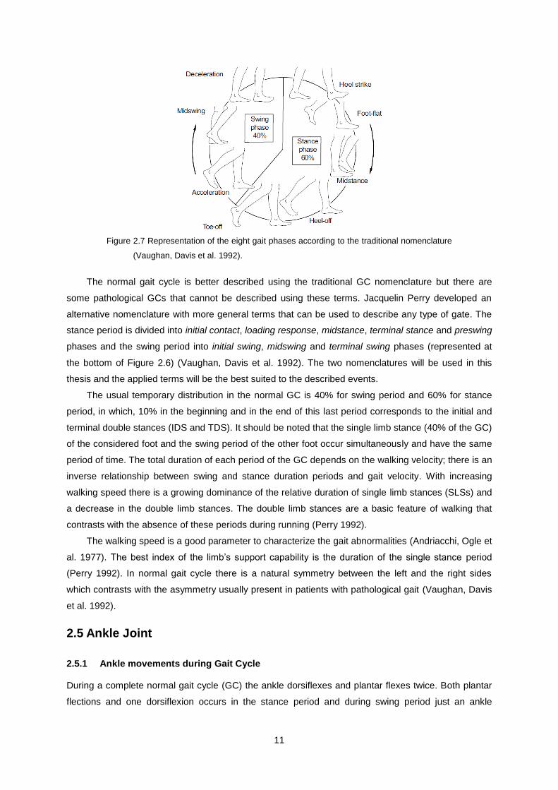
Figure 2.7 Representation of the eight gait phases according to the traditional nomenclature
(Vaughan, Davis et al. 1992). ................................................................................................................ 11
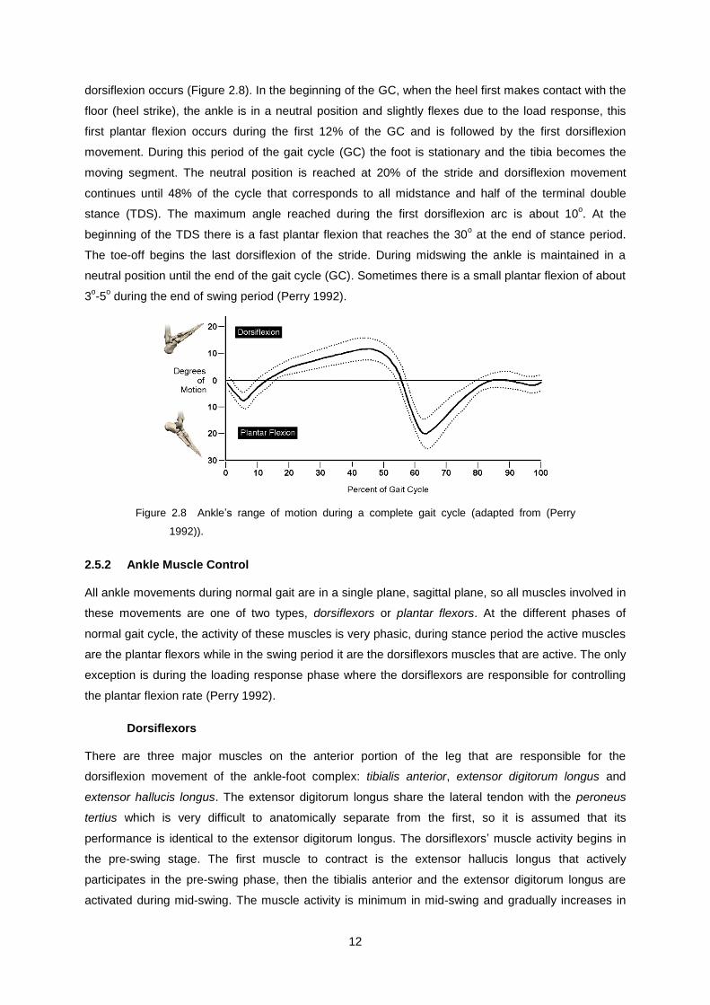
Figure 2.8 Ankle’s range of motion during a complete gait cycle (adapted from (Perry 1992)). .......... 12
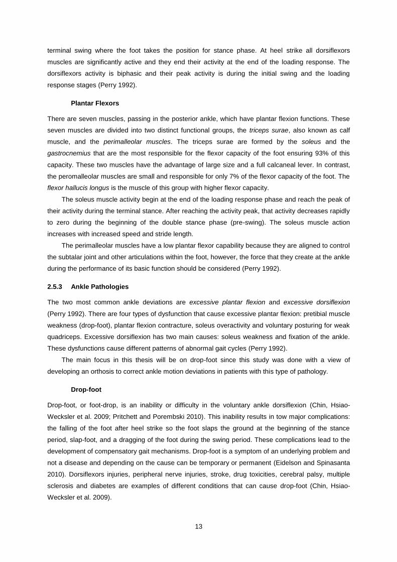
Figure 3.1 Example of two articulated AFOs with plantar flexion stop and free dorsiflexion (Romkes
and Brunner 2002; Fatone, Gard et al. 2009). ...................................................................................... 18
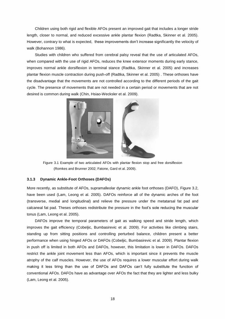
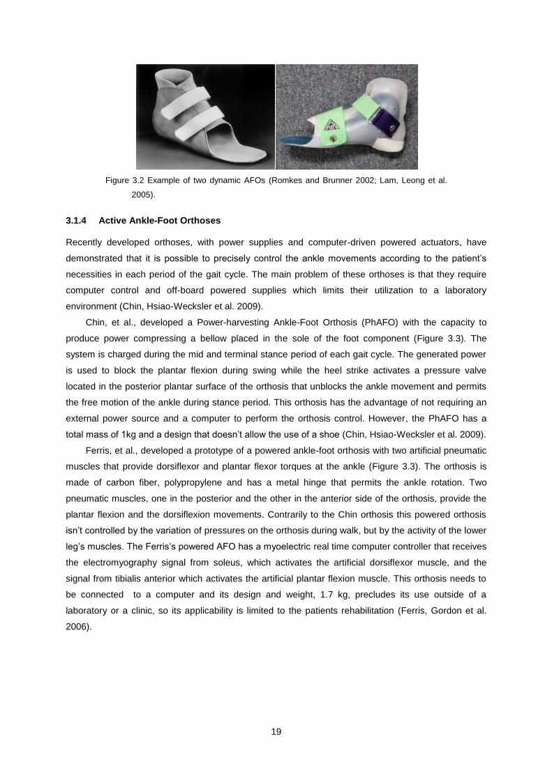
Figure 3.2 Example of two dynamic AFOs (Romkes and Brunner 2002; Lam, Leong et al. 2005). ..... 19
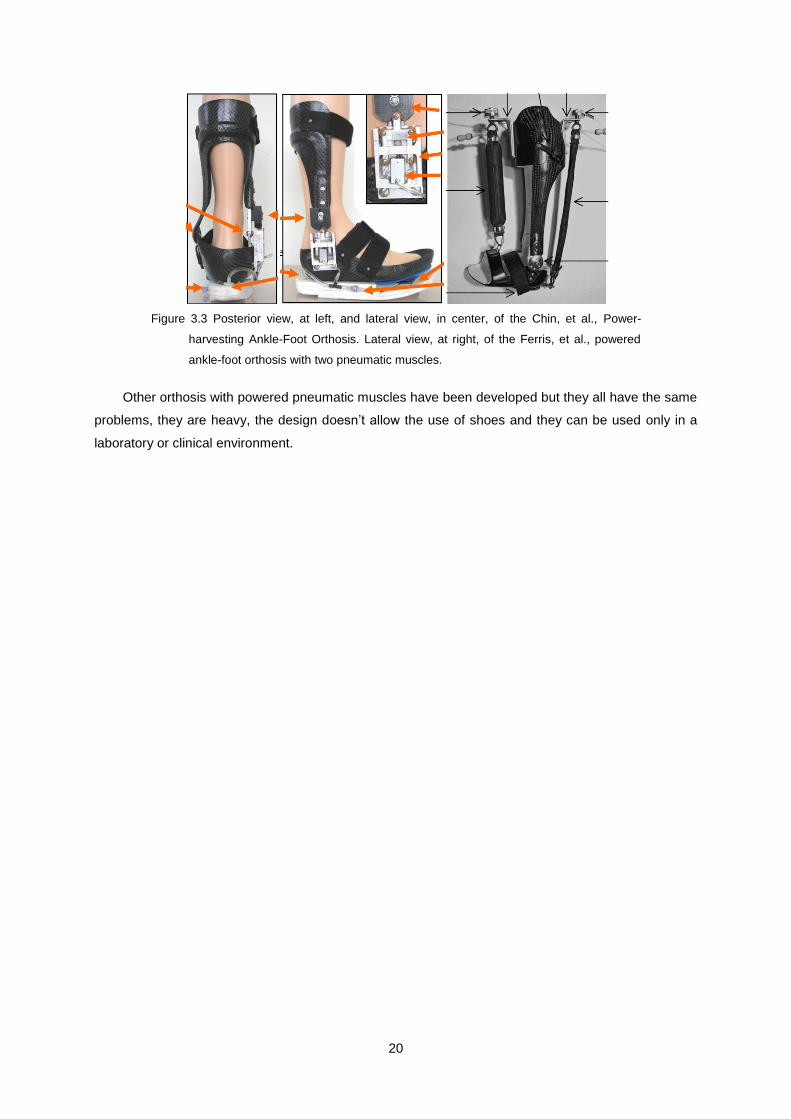
Figure 3.3 Posterior view, at left, and lateral view, in center, of the Chin, et al., Power-harvesting
Ankle-Foot Orthosis. Lateral view, at right, of the Ferris, et al., powered ankle-foot orthosis with two
pneumatic muscles. ............................................................................................................................... 20
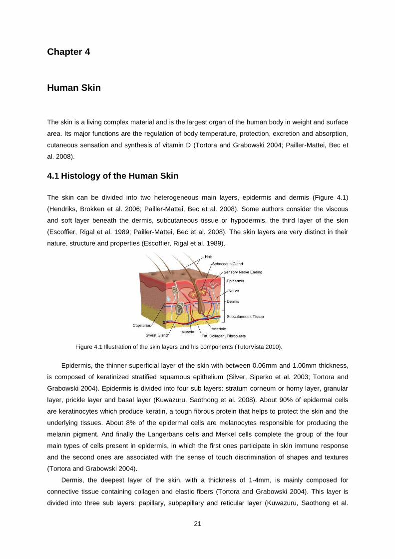
Figure 4.1 Illustration of the skin layers and his components (TutorVista 2010). ................................. 21
Figure 4.2 Representation of the stress-strain curve behavior of human skin in uniaxial tension, on the
left, and in biaxial tension, on the right (Silver, Siperko et al. 2003). .................................................... 23
Figure 4.3 Representation of the Langer’s Lines in anterior (A) and posterior (B) views of the human
body (Dictionary 2010). ......................................................................................................................... 25
Figure 4.4 Schematic representation of the Iberall’s method to draw the directions of the lines of non-
extension (LoNE). At the left, Iberall’s LoNE for the right lower limb. At the right, the warped circle is
represented by a continuous line, the warped ellipse by a dashed line and the LoNE by red dashed
arrows (Bethke 2005). ........................................................................................................................... 26
Figure 4.5 At the left, test done by Iberall, using inextensible cables, to demonstrate that there are
lines on the human body surface that don’t stretch during human motion. At the right, Iberall’s lines of
non-extension for the lower limb (Iberall 1964). .................................................................................... 27
Figure 4.6 Directions of minimum normal strain during knee flexion, obtained by Bethke. A) Anterior
leg’s view. B) Posterior leg’s view (Newman 2005). ............................................................................. 27
Figure 4.7 MIT prototype of the lines of non-extension, made of Kevlar inextensible fibers. A) From left
to right, anterior, lateral and posterior views of the prototype. B) Knee flexion using the MIT prototype
(Newman 2005). .................................................................................................................................... 28
X
Figure 4.8 At left, anterior view of the lines of non-extension of the human’s body (Newman and
Hoffman 2003). At right, Prof. Dava Newman wearing a Bio-Suit mockup (Steger 2005). ................... 28
Figure 5.1 2D representation of polar decomposition of the deformation gradient , eigenvalues and
eigenvectors (Simões 2009). ................................................................................................................. 31
Figure 5.2 a) Representation of a plane state of strain. b) Representation of Mohr’s circle for plane
strain. ..................................................................................................................................................... 32
Figure 6.1 At left, disposition (in arc) of the four infrared cameras and a plastic cube marking the
acquisition volume. The picture was taken during the static calibration of the cameras. At right, one of
the infrared ProReflexTM
MCU500 cameras used in motion capture. ................................................... 33
Figure 6.2 Markers grid on the right foot’s skin of subject 1. From left to right: lateral, medial, posterior
and anterior foot’s view. ......................................................................................................................... 34
Figure 6.3 Typical plantar flexion (TPF), at left, and typical dorsiflexion (TDF), at right. ...................... 35
Figure 6.4 Ground plantar flexion (GPF), at left and ground dorsiflexion (GDF), at right. .................... 36
Figure 6.5 At left, original mesh. At Right, refined mesh where the edge of each element was divided
into four parts. ........................................................................................................................................ 37
Figure 6.6 Schematic representation of the triangular elements in the initial and deformed shape, their
position relatively to the global axis system and the orientation of the element’s positive normal. ...... 38
Figure 7.1 Representation of the longitudinal and circumferential directions on the foot. The red lines
represent the directions defined as longitudinal and the green lines the directions defined as
circumferential (adapted from (Winandy 2009)). ................................................................................... 44
Figure 7.2 At left, principal strains’ field for the typical plantar flexion (TPF) represented in the
deformed configuration 100PF. At right, the directions of minimum strain. Both analyses were
performed with the original mesh (not refined), in the right lateral view and yellow diamond indicates
the lateral malleolus location. ................................................................................................................ 44
Figure 7.3 Right foot’s strains’ field represented in 100TPF configuration (refined mesh, subject 1). At
left, medial view of skin’s strain field, the yellow diamond indicates the medial malleolus. At second
from the left, posterior view of skin’s strain field, the yellow diamond indicates the lateral malleolus. At
third from the left, lateral view of skin’s strain field, the diamond indicates the lateral malleolus. At the
right, anterior view of skin’s strain field. ................................................................................................. 45
Figure 7.4 Right foot’s strains’ field for the 100GPF deformed shape (refined mesh, subject 2). At left,
medial view of skin’s strain field, the diamond indicates the medial malleolus. At right, lateral view of
skin’s strain field, the diamond indicates the lateral malleolus. ............................................................. 46
Figure 7.5 Right foot’s strains’ field represented in 100TDF (complete typical dorsiflexion, subject 1).
At left, medial view of skin’s strain field, the yellow diamond indicates the medial malleolus. At right,
lateral view of skin’s strain field, the diamond indicates the lateral malleolus. ...................................... 47
Figure 7.6 Directions of minimum stretch during 100TPF (right foot, subject 1). Each line of the
crosses corresponds to one direction of non-extension, and each of the single lines corresponds to the
direction of minimum stretch (extension or compression. A) Medial foot’s view, the yellow diamond
corresponds to the medial malleolus. B) Posterior foot’s view, the yellow diamond corresponds to the
XI
lateral malleolus location. C) Lateral foot’s view, the yellow diamond corresponds to the lateral
malleolus location. D) Anterior foot’s view. ............................................................................................ 49
Figure 7.7 Directions of minimum strain during 100TDF (right foot, subject 1). Each line of the crosses
correspond to one direction of non-extension and each of the single lines correspond to the direction
of minimum stretch (extension or compression). At left, medial foot’s view, the yellow diamond
corresponds to the medial malleolus’ location. At right, lateral foot’s view, the yellow diamond
corresponds to the lateral malleolus’ location. ...................................................................................... 53
Figure 7.8 The seven sets of lines of non-extension (LoNE) drawn in the field of minimum strains of
the right foot and distal leg of subject 1. At left, medial foot’s and leg’s view. At center, posterior foot’s
and leg’s view. At right, lateral foot’s and leg’s view. The L1 is represented by the blue lines, L2 by the
orange, L3 by the dark green, L4 by the purple, L5 by the pink, L6 by the brown and the L7 by the light
green lines. The yellow diamond represents the malleolus location. .................................................... 58
Figure 7.9 At upper left, Iberall’s LoNE for the lower limb (Iberall 1970). At upper right, representation
of the anterior view of the Bio-Suit’s LoNE (Newman and Hoffman 2003). At bottom left, medial view of
the right foot’s LoNE obtained in this study. At bottom left, lateral view of the right foot’s LoNE obtained
in this study. ........................................................................................................................................... 60
Figure A. 1 Lateral view of the directions of minimum strain from subject 1. A) 20TPF movement. B)
40TPF movement. C) 60TPF movement. D) 80TPF movement. E) 100TPF movement. .................... 69
Figure B. 1 Right foot’s strains’ field represented in 100TPF (complete typical plantar flexion, refined
mesh, subject 2). At left, medial view of skin’s strain field, the yellow diamond indicates the medial
malleolus. At center, posterior view of skin’s strain field, the green triangle indicates the ~2cm
posterior position the lateral malleolus. At right, lateral view of skin’s strain field, the diamond indicates
the lateral malleolus. .............................................................................................................................. 71
Figure B. 2 Right foot’s strains’ field for the 100GPF deformed shape (refined mesh, subject 1). Lateral
view of skin’s strain field, the diamond indicates the lateral malleolus. ................................................ 71
Figure B. 3 Right foot’s strains’ field represented in 100TDF (complete typical dorsiflexion, refined
mesh, subject 2). At left, medial view of skin’s strain field, the yellow diamond indicates the medial
malleolus. At center, posterior view of skin’s strain field, the green triangle indicates the ~2cm
posterior position the lateral malleolus. At right, lateral view of skin’s strain field, the diamond indicates
the lateral malleolus. .............................................................................................................................. 72
Figure B. 4 Directions of minimum stretch during 100TPF (complete typical plantar flexion, right foot,
subject 2). Each line of the crosses correspond to one direction of non-extension and each of the
single lines correspond to the direction of minimum stretch (extension or compression), when were not
found directions of non-extension on the element. At left, medial foot’s view, the yellow diamond
corresponds to the medial malleolus’ location. At center, posterior foot’s view, the green triangle
indicates the ~2cm posterior position the lateral malleolus. At right, lateral foot’s view, the yellow
diamond corresponds to the lateral malleolus location. ........................................................................ 72
XII
Figure B. 5 Directions of minimum stretch during 100TDF (complete typical dorsiflexion, right foot,
subject 2). Each line of the crosses correspond to one direction of non-extension and each of the
single lines correspond to the direction of minimum stretch (extension or compression), when were not
found directions of non-extension on the element. At left, medial foot’s view, the yellow diamond
corresponds to the medial malleolus’ location. At center, posterior foot’s view, the green triangle
indicates the ~2cm posterior position the lateral malleolus. At right, lateral foot’s view, the yellow
diamond corresponds to the lateral malleolus location. ........................................................................ 73
XIII
List of Tables
Table 6.1 Representation of the three possible cases of skin deformation. The black circle represents
the initial (undeformed) shape, the blue ellipse represents the deformed shape and the orange arrow
the direction(s) of minimum strain for each case. For each case the corresponding Mohr’s circle
representation is presented. .................................................................................................................. 41
Table 7.1 Color code used in the representation of the skin’s strain field and corresponding Mohr’s
circle representation for each strain case. ............................................................................................. 43
Table 7.2 Values of maximum and minimum deformation obtained in 100TPF (complete typical plantar
flexion) for both subjects. ....................................................................................................................... 45
Table 7.3 Values of maximum and minimum deformation obtained in 100TDF (complete typical
dorsiflexion) for both subjects. ............................................................................................................... 47
Table 7.4 Foot and leg regions where the directions of minimum strain are perfectly consistent
between the elements. Identification, illustration and respective anatomical description of the skin’s
regions. Analyses from typical plantar flexion, subject 1. ...................................................................... 50
Table 7.5 Foot and leg regions where the directions of minimum strain have some inconsistencies
between the elements of the original mesh. Identification, illustration and anatomical description of the
skin’s regions. Analyses from typical plantar flexion, subject 1............................................................. 51
Table 7.6 Sets of LoNE obtained for the leg and foot. Lines’ sets identification and medial, posterior
and lateral view of each set, represented in the anatomical reference position. Right foot of the subject
1, directions of minimum strain from 100TPF........................................................................................ 55

XIV

XV
Abbreviations
2D Two-Dimensions
3D Three-Dimensions
20DF 20% of the complete dorsiflexion movement
40DF 40% of the complete dorsiflexion movement
60DF 60% of the complete dorsiflexion movement
80DF 80% of the complete dorsiflexion movement
100DF Complete Dorsiflexion Movement
20PF 20% of the complete plantar flexion movement
40PF 40% of the complete plantar flexion movement
60PF 60% of the complete plantar flexion movement
80PF 80% of the complete plantar flexion movement
100PF Complete Plantar Flexion Movement
AFO Ankle-Foot Orthosis
CMT Charcot-Marie-Tooth
DAFO Dynamic Ankle-Foot Orthosis
DC Direct Current
DoF Degrees of Freedom
FDS First Double Support
FES Functional Electrical Stimulation
GC Gait Cycle
GDF Ground Dorsiflexion
GPF Ground Plantar Flexion
IC Initial Contact
IDS Initial Double Stance
KAFO Knee-Ankle-Foot Orthosis
LoNE Lines of Non-Extension
MIT Massachusetts Institute of Technology
PhAFO Power-harvesting Ankle-Foot Orthosis
QTM Qualisys Track Manager
SLS Single Limb Stance
TDF Typical Dorsiflexion
TDS Terminal Double Stance
TPF Typical Plantar Flexion
USA United States of America
USAF United States Air Force

XVI

XVII
List of Symbols
Occupied region, for a rigid body, at the initial configuration
3D Global Axis System
Time
Point’s position in the Euclidian space at the initial configuration
Point’s position in the Euclidian space at the deformed configuration in time
Function of the particle’s motion
Point’s displacement vector
Relative position between two points at the initial configuration
Length between two points at the initial configuration
Relative position between two points at the deformed configuration
Length between two points at the deformed configuration
Deformation Gradient
c(t) Displacement of the rigid body
Rotation Tensor
Right Stretch Tensor
Left Stretch Tensor
Principal Stretches
Eigenvectors of the Right Stretch Tensor
Eigenvectors of the Left Stretch Tensor
Nominal Strain Tensor (in the deformed configuration)
Identity Tensor
Element’s (identification) Number
Engineering Shear Strain
Element’s Local Axis System
Element’s Strain Tensor
Center of the Circle
Radius of the Circle
Maximum Principal Strain
Minimum Principal Strain
Rotation angle to obtain the principals trains directions
Rotation angle to obtain a direction with a certain strain
Strain value
Marker’s (identification) Number
Element’s Positive Normal in the Initial Configuration (global system)
Element’s Positive Normal in the Deformed Configuration (global system)
Element’s Maximum Principal Direction (local axis system)
Element’s Minimum Principal Direction (local axis system)

XVIII
First Direction of Minimum Strain (in modulus, local axis system)
Second Direction of Minimum Strain (in modulus, local axis system)
1
Chapter 1
1. Introduction
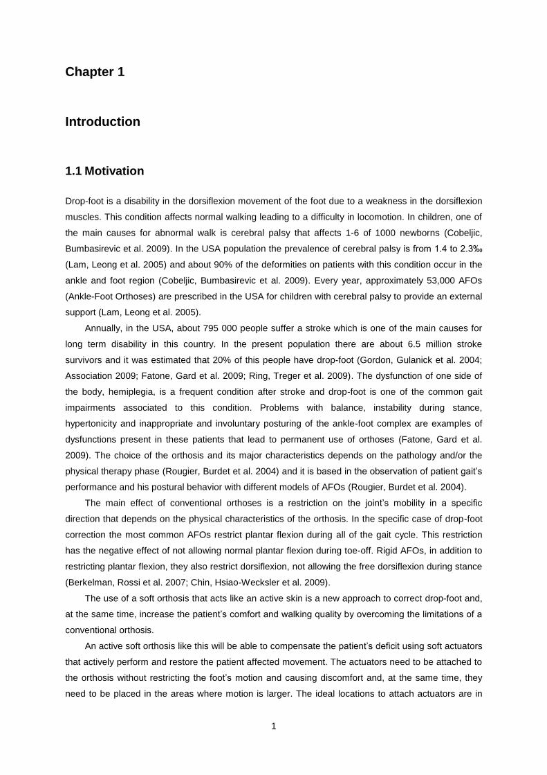
1.1 Motivation
Drop-foot is a disability in the dorsiflexion movement of the foot due to a weakness in the dorsiflexion
muscles. This condition affects normal walking leading to a difficulty in locomotion. In children, one of
the main causes for abnormal walk is cerebral palsy that affects 1-6 of 1000 newborns (Cobeljic,
Bumbasirevic et al. 2009). In the USA population the prevalence of cerebral palsy is from 1.4 to 2.3‰
(Lam, Leong et al. 2005) and about 90% of the deformities on patients with this condition occur in the
ankle and foot region (Cobeljic, Bumbasirevic et al. 2009). Every year, approximately 53,000 AFOs
(Ankle-Foot Orthoses) are prescribed in the USA for children with cerebral palsy to provide an external
support (Lam, Leong et al. 2005).
Annually, in the USA, about 795 000 people suffer a stroke which is one of the main causes for
long term disability in this country. In the present population there are about 6.5 million stroke
survivors and it was estimated that 20% of this people have drop-foot (Gordon, Gulanick et al. 2004;
Association 2009; Fatone, Gard et al. 2009; Ring, Treger et al. 2009). The dysfunction of one side of
the body, hemiplegia, is a frequent condition after stroke and drop-foot is one of the common gait
impairments associated to this condition. Problems with balance, instability during stance,
hypertonicity and inappropriate and involuntary posturing of the ankle-foot complex are examples of
dysfunctions present in these patients that lead to permanent use of orthoses (Fatone, Gard et al.
2009). The choice of the orthosis and its major characteristics depends on the pathology and/or the
physical therapy phase (Rougier, Burdet et al. 2004) and it is based in the observation of patient gait’s
performance and his postural behavior with different models of AFOs (Rougier, Burdet et al. 2004).
The main effect of conventional orthoses is a restriction on the joint’s mobility in a specific
direction that depends on the physical characteristics of the orthosis. In the specific case of drop-foot
correction the most common AFOs restrict plantar flexion during all of the gait cycle. This restriction
has the negative effect of not allowing normal plantar flexion during toe-off. Rigid AFOs, in addition to
restricting plantar flexion, they also restrict dorsiflexion, not allowing the free dorsiflexion during stance
(Berkelman, Rossi et al. 2007; Chin, Hsiao-Wecksler et al. 2009).
The use of a soft orthosis that acts like an active skin is a new approach to correct drop-foot and,
at the same time, increase the patient’s comfort and walking quality by overcoming the limitations of a
conventional orthosis.
An active soft orthosis like this will be able to compensate the patient’s deficit using soft actuators
that actively perform and restore the patient affected movement. The actuators need to be attached to
the orthosis without restricting the foot’s motion and causing discomfort and, at the same time, they
need to be placed in the areas where motion is larger. The ideal locations to attach actuators are in
2
places where we can place inextensible wires without restring the foot’s motions. Arthur Iberall
introduced the concept of lines of non-extension (LoNE), lines on the skin that, during human motion,
only suffer distortion and no deformation. These lines are the ideal places to pass the orthosis’
inextensible wires (Iberall 1964). To identify the locations of the LoNE it is necessary to map the skin’s
train field and calculate the orientations of these lines.
1.2 Objectives
The purpose of this thesis is to obtain the skin strain field map at the ankle joint by calculating the
directions and magnitudes of the principal strains and finding the directions of the lines of non-
extension (LoNE). The results shall provide useful information for the development of a new active
orthosis that will act as a second skin in the drop-foot correction. In this study, we determine the
direction of the skin’s lines where inextensible wires for the orthosis actuators’ attachment can be
placed without restricting foot’s motion, and we identify the skin’s areas where larger deformation
exists during the normal gait cycle. The directions and magnitudes of the principal strains provide
important information for the orthosis actuators’ location and for their performance throughout the
different periods of the gait cycle.
1.3 Literature Review
Drop-foot is a condition where the dorsiflexion movement is compromised due to a weakness in the
dorsiflexors muscles. This condition has as principal causes: dorsiflexors injuries, peripheral nerve
injuries, stroke, cerebral palsy, multiple sclerosis and diabetes (Chin, Hsiao-Wecksler et al. 2009).
People with drop-foot have a pathological gait characterized by the lack of dorsiflexion during
swing period and a foot slap in the initial stance, more precisely, in heel strike (Geboers, Drost et al.
2002). This inability to perform dorsiflexion leads to the development of compensatory gait
mechanisms in order to avoid the dragging toe on the ground. People with drop-foot have a larger flex
movement of the hip during swing period and a lower walking velocity, cadence and step length (Don,
Serrao et al. 2007). There are three main approaches for the drop-foot correction: the use of ankle-
foot orthoses (AFOs), functional electrical stimulation (FES) and tendon transfer from the posterior
tibial muscle (Simonsen, Moesby et al. 2010). The AFOs are the main focus of this work.
Traditionally AFOs for drop-foot correction consists in a unique orthotic piece of material that
maintains the foot in a zero angle position (anatomic reference position) in order to stop plantar
flexion. This type of AFOs, besides correcting drop-foot, also restrict foot’s movements that aren’t
affected, like plantar flexion in pre-swing and passive dorsiflexion during mid-stance which leads to an
unnatural gait (Berkelman, Rossi et al. 2007; Chin, Hsiao-Wecksler et al. 2009). Articulated AFOs are
an alternative to rigid AFOs, they act like rigid AFOs in the plantar flexion stop but they allow passive
dorsiflexion during mid-stance; however they also don’t allow normal plantar flexion in pre-swing
(Radtka, Skinner et al. 2005).
A new alternative to traditional orthoses, which is still in development, are the active orthoses.
Active orthoses are powered orthoses that produce motion to help patients to perform the normal
3
segment’s movements during walking for each gait cycle period. The first patent of an active orthosis
is from 1935. It was a leg brace that elevates the knee using a crank at the hip. The first controllable
active orthosis is from 1942. It was a hydraulic-actuated orthosis that added power at the hip and knee
(Dollar and Hugh Herr 2007). In 1981 an active ankle-foot orthosis (AFO), was presented by Jaukovic,
which has a DC motor placed in an anterior position to the user’s leg that performs ankle’s flexion and
extension. Ferris’s powered AFO with two artificial pneumatic muscles (Ferris, Gordon et al. 2006),
Chin’s power-harvesting AFO (Chin, Hsiao-Wecksler et al. 2009) and MIT active AFO (Blaya and Herr
2004) are some examples of the most recent developments in this area. Most of these new orthoses
are still confined to a laboratory use due to its dependency from an external computer control,
powered supplies and their weight (Chin, Hsiao-Wecksler et al. 2009).
In the design of a new medical device that contacts with the skin it is important to have in
consideration the skin-device interface (Kwiatkowska, Franklin et al. 2009). The shear stress at the
skin-device interface leads to repeated micro-traumas that can result in chronic wounding (Sanders,
Goldstein et al. 1995; Holt, Tripathi et al. 2008). Many studies about the skin’s biomechanical
properties have been made. In 1861, Karl Lenger was the first to report that skin’s collagen fibrils have
a natural orientation. He mapped the lines of maximum pre-stress in the human body, through
punched out circular holes on cadavers for observing the directions of the ellipses in which they
became (Langer 1978). The oldest in vivo studies to measure skin’s deformation were performed by
measuring the uni- and bi-axial tension (Abas 1982; Abas 1994). More recent studies, using 3D
motion capture, directly measure skin’s deformation (Bethke 2005; Mahmud, Holt et al. 2010).
In the late sixties, Arthur Iberall was the first to suggest the existence of a network of non-extension
lines covering all human skin’s surface. He noticed that in some skin’s directions, during human
motion, distortion and no deformation are suffered. Iberall, during his research in the US Air force,
proved that we can pass inextensible wires over these skin’s lines without restrict the free human
motion (Iberall 1964). Following Iberall, a master student Kristen Bethke at MIT, using more
sophisticate methods for acquisition and analysis of the human skin strain, mapped the lines of non-
extension in the leg (Bethke 2005). Both Iberall and Bethke studies were conducted with a view to
improve mobility in astronauts’ spacesuits and none of them studied the strains field at the human
ankle.
The work developed in this thesis is the first to map the network of lines of non-extension about
the human ankle and the only one that used this approach for the development of a new orthosis that
acts like a second skin.
1.4 Contributions
The contributions of this thesis are:
To implement a computational routine that automates the analysis of the principals’ strains
field and minimum strains field of the skin.
To map the foot and ankle skin’s strains field for both plantar flexion and dorsiflexion
movements.
4
To identify the directions in the foot and ankle’s surface where the skin doesn’t deform, during
the walk.
1.5 Thesis Organization
This thesis is organized in 8 chapters. In the first chapter the motivation and objectives of this thesis
are presented as well as a review of the work that was done in this area. In chapter 2 the human gait
motion is described giving greater emphasis to the analyses of the lower limb, in particular, the ankle
joint. In chapter 3 the existing AFOs for drop-foot correction and their characteristics, advantages and
disadvantages are presented. In chapter 4 the anatomical and biomechanical skin’s characteristics
and important skin’s studies for the development of this thesis are presented. In chapter 5 the strain
calculus theory is presented. The entire laboratorial procedure, data acquisition and computational
analysis are described in chapter 6. The results from this study and their discussion are presented in
chapter 7. In chapter 8 the most important conclusions of this thesis are presented and possible
guidelines for future works are suggested.
This work was developed under the scope of the FCT project DACHOR-Multibody Dynamics And
Control of Active Hybrid Orthoses (MIT-Pt/BS-HHMS/0042/2008).
5
Chapter 2
2. Human Motion
2.1 Lower limb’s anatomy
The lower limb (Figure 2.1) is divided in three different anatomic segments: thigh, leg and foot. The
femur is the only bone in the thigh and is the longer and most voluminous bone of the human body.
The patella, the tibia and the fibula are the three leg’s bones. The patella is a small and triangular
bone with an anterior location to the distal femur and to the proximal tibia and is known as the knee
joint. The tibia is the larger medial leg’s bone that bears the body weight. At its proximal end the tibia
articulates with the femur and the fibula, and at its distal end with the fibula and the ankle’s talus. The
proximal tibia’s extremity expands into a lateral and a medial condyle and the surface of the medial
distal extremity forms the medial malleolus. The fibula is parallel and lateral to the tibia, its proximal
extremity articulates with the tibia’s lateral condyle and the distal extremity has a projection called
lateral malleolus. Both lateral and medial malleolus articulate with the ankle’s talus (Tortora and
Grabowski 2004).
Figure 2.1 At left, representation of the lower limb’s bones, extracted from (UK 2010). At
right, representation of the foot’s bones, extracted from (Britannica 2007).
The tarsus, or ankle, is formed by seven bones, called the tarsals, held by ligaments. The
calcaneus and the talus are located at the foot’s posterior part. The cuboid, navicular, and the three
cuneiform bones (first, second and third cuneiforms) form the anterior ankle’s part. The calcaneus is
the largest and the strongest tarsal. The metatarsals’ bones are numbered from one to five from the
medial to the lateral position and they have an anterior position to the tarsals. The foot’s phalanges
6
have an anterior position to the metatarsals. The great toe, or big toe, is formed by two phalange, the
other four toes are formed by three phalanges each (proximal, medial and distal phalange) (Tortora
and Grabowski 2004).
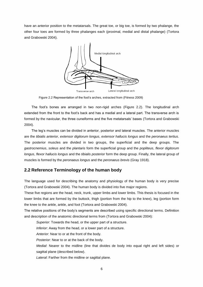
Figure 2.2 Representation of the foot’s arches, extracted from (Fitness 2009)
The foot’s bones are arranged in two non-rigid arches (Figure 2.2). The longitudinal arch
extended from the front to the foot’s back and has a medial and a lateral part. The transverse arch is
formed by the navicular, the three cuneiforms and the five metatarsals’ bases (Tortora and Grabowski
2004).
The leg’s muscles can be divided in anterior, posterior and lateral muscles. The anterior muscles
are the tibialis anterior, extensor digitorum longus, extensor hallucis longus and the peronaeus tertius.
The posterior muscles are divided in two groups, the superficial and the deep groups. The
gastrocnemius, soleus and the plantaris form the superficial group and the popliteus, flexor digitorum
longus, flexor hallucis longus and the tibialis posterior form the deep group. Finally, the lateral group of
muscles is formed by the peronaeus longus and the peronaeus brevis (Gray 1918).
2.2 Reference Terminology of the human body
The language used for describing the anatomy and physiology of the human body is very precise
(Tortora and Grabowski 2004). The human body is divided into five major regions.
These five regions are the head, neck, trunk, upper limbs and lower limbs. This thesis is focused in the
lower limbs that are formed by the buttock, thigh (portion from the hip to the knee), leg (portion form
the knee to the ankle, ankle, and foot (Tortora and Grabowski 2004).
The relative positions of the body’s segments are described using specific directional terms. Definition
and description of the anatomic directional terms from (Tortora and Grabowski 2004):
Superior: Towards the head, or the upper part of a structure.
Inferior: Away from the head, or a lower part of a structure.
Anterior: Near to or at the front of the body.
Posterior: Near to or at the back of the body.
Medial: Nearer to the midline (line that divides de body into equal right and left sides) or
sagittal plane (described below).
Lateral: Farther from the midline or sagittal plane.
7
Proximal: Nearer to the attachment of a limb to the trunk, near to the point of origin or the
beginning.
Distal: Farther to the attachment of a limb to the trunk, farther from the point of origin or the
beginning.
Superficial: Toward or on the surface of the body.
Deep: Away from the surface of the body.
All human motions are described relative to the anatomical reference position, anatomical
reference planes and anatomical reference axes using specific direction terms.
By convention the body in the anatomical position reference is in an erect standing position with
the arms hanging relaxed at the body sides, the palms of the hands facing forwards and the feet
slightly apart (Figure 2.3) (Hall 1991).
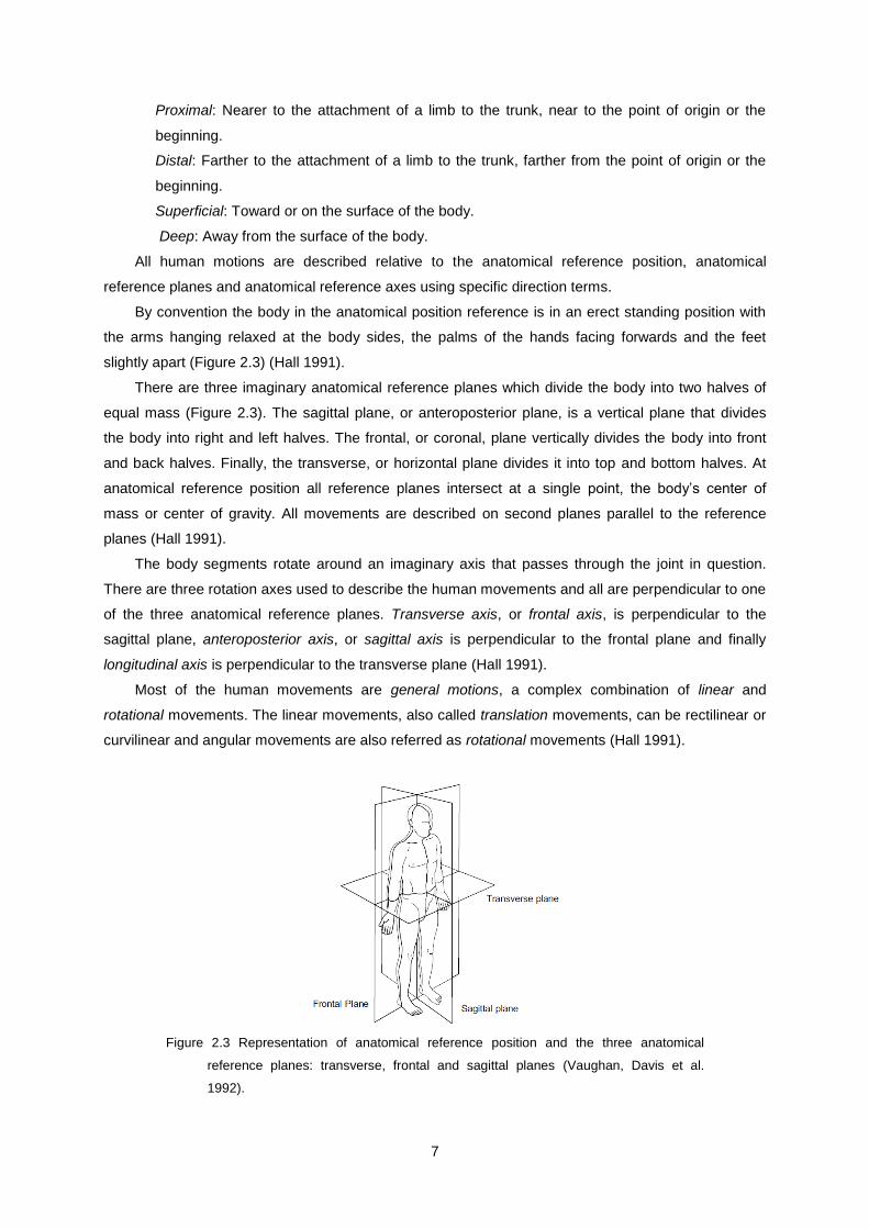
There are three imaginary anatomical reference planes which divide the body into two halves of
equal mass (Figure 2.3). The sagittal plane, or anteroposterior plane, is a vertical plane that divides
the body into right and left halves. The frontal, or coronal, plane vertically divides the body into front
and back halves. Finally, the transverse, or horizontal plane divides it into top and bottom halves. At
anatomical reference position all reference planes intersect at a single point, the body’s center of
mass or center of gravity. All movements are described on second planes parallel to the reference
planes (Hall 1991).
The body segments rotate around an imaginary axis that passes through the joint in question.
There are three rotation axes used to describe the human movements and all are perpendicular to one
of the three anatomical reference planes. Transverse axis, or frontal axis, is perpendicular to the
sagittal plane, anteroposterior axis, or sagittal axis is perpendicular to the frontal plane and finally
longitudinal axis is perpendicular to the transverse plane (Hall 1991).
Most of the human movements are general motions, a complex combination of linear and
rotational movements. The linear movements, also called translation movements, can be rectilinear or
curvilinear and angular movements are also referred as rotational movements (Hall 1991).
Figure 2.3 Representation of anatomical reference position and the three anatomical
reference planes: transverse, frontal and sagittal planes (Vaughan, Davis et al.
1992).
8
2.3 Terminology of the Joint’s Movements
By convention all body segments are considered at zero degrees in the anatomical reference position.
The rotation movements of the body segments are named according to the motion direction and
measured according to the angle formed between the body segment’s position and anatomical
position (Hall 1991).
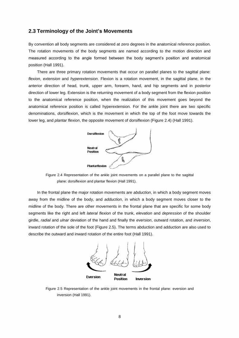
There are three primary rotation movements that occur on parallel planes to the sagittal plane:
flexion, extension and hyperextension. Flexion is a rotation movement, in the sagittal plane, in the
anterior direction of head, trunk, upper arm, forearm, hand, and hip segments and in posterior
direction of lower leg. Extension is the returning movement of a body segment from the flexion position
to the anatomical reference position, when the realization of this movement goes beyond the
anatomical reference position is called hyperextension. For the ankle joint there are two specific
denominations, dorsiflexion, which is the movement in which the top of the foot move towards the
lower leg, and plantar flexion, the opposite movement of dorsiflexion (Figure 2.4) (Hall 1991).
Figure 2.4 Representation of the ankle joint movements on a parallel plane to the sagittal
plane: dorsiflexion and plantar flexion (Hall 1991).
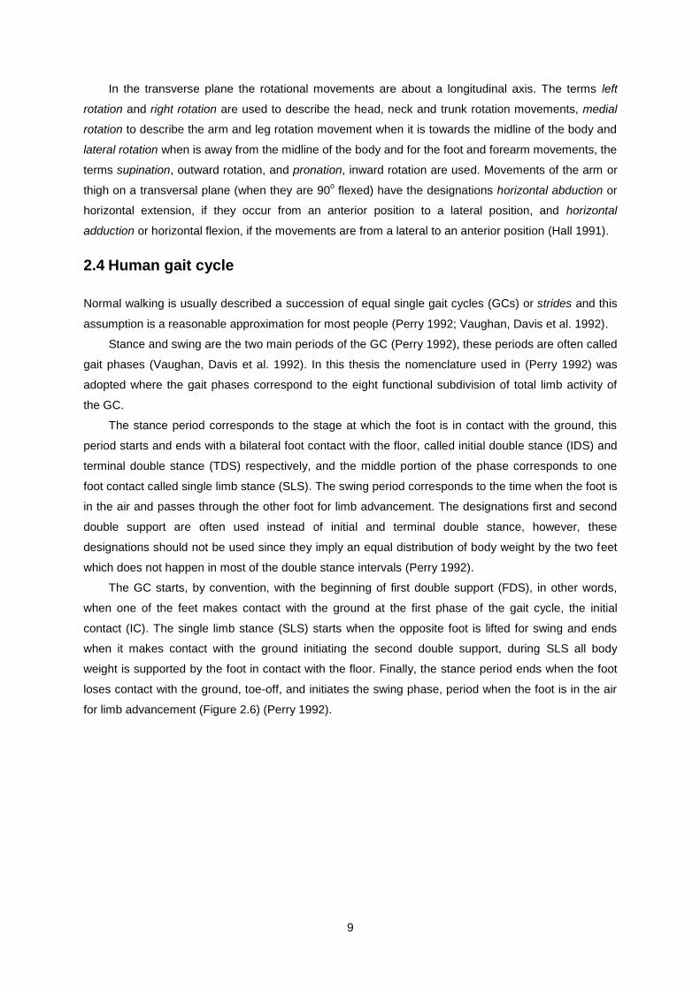
In the frontal plane the major rotation movements are abduction, in which a body segment moves
away from the midline of the body, and adduction, in which a body segment moves closer to the
midline of the body. There are other movements in the frontal plane that are specific for some body
segments like the right and left lateral flexion of the trunk, elevation and depression of the shoulder
girdle, radial and ulnar deviation of the hand and finally the eversion, outward rotation, and inversion,
inward rotation of the sole of the foot (Figure 2.5). The terms abduction and adduction are also used to
describe the outward and inward rotation of the entire foot (Hall 1991).
Figure 2.5 Representation of the ankle joint movements in the frontal plane: eversion and
inversion (Hall 1991).
9
In the transverse plane the rotational movements are about a longitudinal axis. The terms left
rotation and right rotation are used to describe the head, neck and trunk rotation movements, medial
rotation to describe the arm and leg rotation movement when it is towards the midline of the body and
lateral rotation when is away from the midline of the body and for the foot and forearm movements, the
terms supination, outward rotation, and pronation, inward rotation are used. Movements of the arm or
thigh on a transversal plane (when they are 90o flexed) have the designations horizontal abduction or
horizontal extension, if they occur from an anterior position to a lateral position, and horizontal
adduction or horizontal flexion, if the movements are from a lateral to an anterior position (Hall 1991).
2.4 Human gait cycle
Normal walking is usually described a succession of equal single gait cycles (GCs) or strides and this
assumption is a reasonable approximation for most people (Perry 1992; Vaughan, Davis et al. 1992).
Stance and swing are the two main periods of the GC (Perry 1992), these periods are often called
gait phases (Vaughan, Davis et al. 1992). In this thesis the nomenclature used in (Perry 1992) was
adopted where the gait phases correspond to the eight functional subdivision of total limb activity of
the GC.
The stance period corresponds to the stage at which the foot is in contact with the ground, this
period starts and ends with a bilateral foot contact with the floor, called initial double stance (IDS) and
terminal double stance (TDS) respectively, and the middle portion of the phase corresponds to one
foot contact called single limb stance (SLS). The swing period corresponds to the time when the foot is
in the air and passes through the other foot for limb advancement. The designations first and second
double support are often used instead of initial and terminal double stance, however, these
designations should not be used since they imply an equal distribution of body weight by the two feet
which does not happen in most of the double stance intervals (Perry 1992).
The GC starts, by convention, with the beginning of first double support (FDS), in other words,
when one of the feet makes contact with the ground at the first phase of the gait cycle, the initial
contact (IC). The single limb stance (SLS) starts when the opposite foot is lifted for swing and ends
when it makes contact with the ground initiating the second double support, during SLS all body
weight is supported by the foot in contact with the floor. Finally, the stance period ends when the foot
loses contact with the ground, toe-off, and initiates the swing phase, period when the foot is in the air
for limb advancement (Figure 2.6) (Perry 1992).

10
Figure 2.6 Representation of the normal gait cycle in a eight years old boy (Vaughan, Davis
et al. 1992).
Depending on the author there are different nomenclatures for the eight phases of the human
GC. Traditionally, the stance period is divided into five phases and the swing period into three phases.
These phase designations are based in the movement of the foot and the traditional nomenclature
(Vaughan, Davis et al. 1992) is described above and represented in Figure 2.7.
Phases of Stance Period
Heel strike: Marks the beginning of gait cycle and correspond to the moment where the body’s
center of gravity is at the lowest position.
Foot-flat: Time when the plantar surface of the foot touches de ground.
Midstance: Corresponds to the point when the swinging foot passes the stance foot. At this point
the body’s gravity center is in the highest position.
Heel-off: Moment when the heel loses contact with the ground.
Toe-off: Corresponds to the end of stance period, the foot loses the contact with the ground.
Phases of Swing Period
Acceleration: It begins when the foot leaves the ground and the hip flexor muscles are activated to
accelerate the leg forward.
Midswing: Point when the foot passes directly besides the stance leg. Occurs at the same time of
contralateral’s foot midstance.
Deceleration: Time when the muscles action results in a deceleration of leg movement and in a foot
stabilization for the next heel strike.
11
Figure 2.7 Representation of the eight gait phases according to the traditional nomenclature
(Vaughan, Davis et al. 1992).
The normal gait cycle is better described using the traditional GC nomenclature but there are
some pathological GCs that cannot be described using these terms. Jacquelin Perry developed an
alternative nomenclature with more general terms that can be used to describe any type of gate. The
stance period is divided into initial contact, loading response, midstance, terminal stance and preswing
phases and the swing period into initial swing, midswing and terminal swing phases (represented at
the bottom of Figure 2.6) (Vaughan, Davis et al. 1992). The two nomenclatures will be used in this
thesis and the applied terms will be the best suited to the described events.
The usual temporary distribution in the normal GC is 40% for swing period and 60% for stance
period, in which, 10% in the beginning and in the end of this last period corresponds to the initial and
terminal double stances (IDS and TDS). It should be noted that the single limb stance (40% of the GC)
of the considered foot and the swing period of the other foot occur simultaneously and have the same
period of time. The total duration of each period of the GC depends on the walking velocity; there is an
inverse relationship between swing and stance duration periods and gait velocity. With increasing
walking speed there is a growing dominance of the relative duration of single limb stances (SLSs) and
a decrease in the double limb stances. The double limb stances are a basic feature of walking that
contrasts with the absence of these periods during running (Perry 1992).
The walking speed is a good parameter to characterize the gait abnormalities (Andriacchi, Ogle et
al. 1977). The best index of the limb’s support capability is the duration of the single stance period
(Perry 1992). In normal gait cycle there is a natural symmetry between the left and the right sides
which contrasts with the asymmetry usually present in patients with pathological gait (Vaughan, Davis
et al. 1992).
2.5 Ankle Joint
2.5.1 Ankle movements during Gait Cycle
During a complete normal gait cycle (GC) the ankle dorsiflexes and plantar flexes twice. Both plantar
flections and one dorsiflexion occurs in the stance period and during swing period just an ankle
12
dorsiflexion occurs (Figure 2.8). In the beginning of the GC, when the heel first makes contact with the
floor (heel strike), the ankle is in a neutral position and slightly flexes due to the load response, this
first plantar flexion occurs during the first 12% of the GC and is followed by the first dorsiflexion
movement. During this period of the gait cycle (GC) the foot is stationary and the tibia becomes the
moving segment. The neutral position is reached at 20% of the stride and dorsiflexion movement
continues until 48% of the cycle that corresponds to all midstance and half of the terminal double
stance (TDS). The maximum angle reached during the first dorsiflexion arc is about 10o. At the
beginning of the TDS there is a fast plantar flexion that reaches the 30o at the end of stance period.
The toe-off begins the last dorsiflexion of the stride. During midswing the ankle is maintained in a
neutral position until the end of the gait cycle (GC). Sometimes there is a small plantar flexion of about
3o-5
o during the end of swing period (Perry 1992).
Figure 2.8 Ankle’s range of motion during a complete gait cycle (adapted from (Perry
1992)).
2.5.2 Ankle Muscle Control
All ankle movements during normal gait are in a single plane, sagittal plane, so all muscles involved in
these movements are one of two types, dorsiflexors or plantar flexors. At the different phases of
normal gait cycle, the activity of these muscles is very phasic, during stance period the active muscles
are the plantar flexors while in the swing period it are the dorsiflexors muscles that are active. The only
exception is during the loading response phase where the dorsiflexors are responsible for controlling
the plantar flexion rate (Perry 1992).
Dorsiflexors
There are three major muscles on the anterior portion of the leg that are responsible for the
dorsiflexion movement of the ankle-foot complex: tibialis anterior, extensor digitorum longus and
extensor hallucis longus. The extensor digitorum longus share the lateral tendon with the peroneus
tertius which is very difficult to anatomically separate from the first, so it is assumed that its
performance is identical to the extensor digitorum longus. The dorsiflexors’ muscle activity begins in
the pre-swing stage. The first muscle to contract is the extensor hallucis longus that actively
participates in the pre-swing phase, then the tibialis anterior and the extensor digitorum longus are
activated during mid-swing. The muscle activity is minimum in mid-swing and gradually increases in
13
terminal swing where the foot takes the position for stance phase. At heel strike all dorsiflexors
muscles are significantly active and they end their activity at the end of the loading response. The
dorsiflexors activity is biphasic and their peak activity is during the initial swing and the loading
response stages (Perry 1992).
Plantar Flexors
There are seven muscles, passing in the posterior ankle, which have plantar flexion functions. These
seven muscles are divided into two distinct functional groups, the triceps surae, also known as calf
muscle, and the perimalleolar muscles. The triceps surae are formed by the soleus and the
gastrocnemius that are the most responsible for the flexor capacity of the foot ensuring 93% of this
capacity. These two muscles have the advantage of large size and a full calcaneal lever. In contrast,
the peromalleolar muscles are small and responsible for only 7% of the flexor capacity of the foot. The
flexor hallucis longus is the muscle of this group with higher flexor capacity.
The soleus muscle activity begin at the end of the loading response phase and reach the peak of
their activity during the terminal stance. After reaching the activity peak, that activity decreases rapidly
to zero during the beginning of the double stance phase (pre-swing). The soleus muscle action
increases with increased speed and stride length.
The perimalleolar muscles have a low plantar flexor capability because they are aligned to control
the subtalar joint and other articulations within the foot, however, the force that they create at the ankle
during the performance of its basic function should be considered (Perry 1992).
2.5.3 Ankle Pathologies
The two most common ankle deviations are excessive plantar flexion and excessive dorsiflexion
(Perry 1992). There are four types of dysfunction that cause excessive plantar flexion: pretibial muscle
weakness (drop-foot), plantar flexion contracture, soleus overactivity and voluntary posturing for weak
quadriceps. Excessive dorsiflexion has two main causes: soleus weakness and fixation of the ankle.
These dysfunctions cause different patterns of abnormal gait cycles (Perry 1992).
The main focus in this thesis will be on drop-foot since this study was done with a view of
developing an orthosis to correct ankle motion deviations in patients with this type of pathology.
Drop-foot
Drop-foot, or foot-drop, is an inability or difficulty in the voluntary ankle dorsiflexion (Chin, Hsiao-
Wecksler et al. 2009; Pritchett and Porembski 2010). This inability results in tow major complications:
the falling of the foot after heel strike so the foot slaps the ground at the beginning of the stance
period, slap-foot, and a dragging of the foot during the swing period. These complications lead to the
development of compensatory gait mechanisms. Drop-foot is a symptom of an underlying problem and
not a disease and depending on the cause can be temporary or permanent (Eidelson and Spinasanta
2010). Dorsiflexors injuries, peripheral nerve injuries, stroke, drug toxicities, cerebral palsy, multiple
sclerosis and diabetes are examples of different conditions that can cause drop-foot (Chin, Hsiao-
Wecksler et al. 2009).

14
A study realized by Romildo Don, et al., in patients with Charcot-Marie-Tooth (CMT) analyzed in
detail the change in gait caused by drop-foot. CMT is a genetic disease that affects the nerves which
control the muscles. The muscles in the body extremities become weakened due to the loss of
stimulation in the effected nerves (Association 2010). Drop-foot and plantar flexion failure are common
pathologies in patients with CMT and we could analyze the gait cycle of these patients in order to
characterize the gait changes present in these pathologies (Don, Serrao et al. 2007).
This study shows that the patients suffering from drop-foot and plantar flexion failure display
characteristic gait changes due to the functional deficits. The most significant differences between
patients affected by drop-foot and plantar flexion failure and patients without pathological gait are at
the kinematic and the kinetic performance of the ankle. In the pathological gait group a decrease in
step length, cadence and swing velocity was observed. Both the swing and the stance phase are
affected in these patients. In order to maintain an adequate step length the patients perform a large
dorsiflexion movement during stance phase due to the excessively plantar flexed ankle at the
beginning of the loading response phase, this dorsiflexion movement is obtained restricting the plantar
flexor angular impulse which in turn limits the ankle dorsiflexion during mid-stance. The changes
observed at the ankle explain the low values of ankle plantar flexion during toe-off and the request of
both cotralateral hip extensor angular impulse and ipsilateral hip flexor angular impulse. This study
also revealed that patients with only drop-foot and patients with both drop-foot and plantar flexion
failure developed different compensatory gait mechanisms (Don, Serrao et al. 2007).
Patient with only drop-foot pathology display a lack of dorsiflexors angular impulse resulting in an
uncontrolled landing of the foot on the floor, slap-foot, during the load response phase. At mid-stance
phase the passive ankle dorsiflexion is increased in order to maintain the body progression, this
increased dorsiflexion is obtained by delaying the plantar flexor muscles activation which culminates in
a reduction of plantar flexor angular impulse. In addition to these changes an increase in hip extension
and a higher knee angular impulse value during stance are also observed. The greater hip extension
is necessary to compensate the increased dorsiflexion in order to maintain the body progress and
balance. The necessary propulsive energy to the toe-off is obtained by an increased plantar flexion
angular impulse during push-off and an increase in hip angular impulse which is also important in the
enhanced hip flexion during swing phase. During swing phase, patients present an increased hip and
knee flexion in order to compensate the characteristic drop-foot in this phase. This motor strategy
performed by the patients is reflected in a larger duration of the swing period, however, the step length
is maintained in normal values. Another consequence of this compensatory gait strategy is the
increased energy consumption during walk (Don, Serrao et al. 2007).
Patients with both drop-foot and plantar flexion failure have some different compensatory gait
strategies from patients who only have drop-foot. As in the previous group these patients also have an
excessively plantar flexed ankle at the initial contact but with a lower angle degree and they use their
hip extensor muscles more than their knee extensors to perform load acceptance. Other similar
features in both groups are the increase of passive dorsiflexion during mid-stance and the decrease of
the plantar flexor angular impulse, however these characteristics are more pronounced in this group
due to the plantar flexor failure. The decrease of hip extension can be explained by the failure of the

15
decelerating action of the plantar flexors which leads to a restriction on the body forwards progression
in order to maintain the anterior-posterior balance. The plantar flexor failure is clearly noticed during
push-off sub-phase where there is a marked decrease in both angular impulse and plantar flexion
range of motion which is, considering the body support, partly compensated by the increased knee
extensor angular impulse. In contrast to the previous group there is not an increase of the hip flexor
angular impulse to compensate the propulsion deficit which is probably due to the different
compensatory gait adopted during swing phase. When compared with the patients from last group
they present a reduced hip and knee flexion during swing phase and an increased hip abduction and
pelvic elevation during swing phase. These compensatory gait mechanism lead to a very slow gait
characterized by a reduced step length and reduced cadence and a broad support area. In relation to
energy expenditure, when compared with previous group, there is a greater energy recovery and a
lower energy consumption (Don, Serrao et al. 2007).

16

17
Chapter 3
3. Ankle-Foot Orthoses (AFO)
3.1 Ankle-Foot Orthoses
An orthosis is an external device, designed to control or correct the movement of a body member
affected from a morphological alteration or a function deficit. An efficient orthosis should only interfere
in the control and improvement of the movement that is compromised by a functional deficit, without
interfering with the other movements (Chin, Hsiao-Wecksler et al. 2009). The first foot orthoses just
restricted the foot’s freedom of movements in order to keep the foot in a desired position and
redistributed the weight-bearing to improve comfort and protection (Lockard 1988).
3.1.1 Rigid Ankle Foot Orthoses (AFOs)
Rigid orthoses are prescribed to passively control the dynamics of the ankle both in the stance and
swing phases (Lam, Leong et al. 2005; Cobeljic, Bumbasirevic et al. 2009). Rigid AFOs, also called
fixed or solid AFOs, keep the foot in an adequate dorsiflexion angle and restrict the plantar flexion
movement (Radtka, Skinner et al. 2005; Cobeljic, Bumbasirevic et al. 2009). The performance of these
orthoses is dependent of the material properties, and their geometry defines the characteristics of the
motion control (Chin, Hsiao-Wecksler et al. 2009). These orthoses limit the normal forward movement
of the tibia during stance, resulting in an excessive plantar flexion and an earlier heel rise during the
stance period (Radtka, Skinner et al. 2005).
Rigid AFOs are made of thermoplastic materials (Cobeljic, Bumbasirevic et al. 2009) such as
polypropylene (Radtka, Skinner et al. 2005). This material and the rigid AFOs design doesn’t allow
free motion of the foot (Chin, Hsiao-Wecksler et al. 2009). Conventional AFOs have a weight between
300-600 g, and require the use of a shoe (Chin, Hsiao-Wecksler et al. 2009).
3.1.2 Articulated Ankle-Foot Orthoses
In some syndromes or diseases like Charcot-Marie-Tooth (CMT), drop-foot is usually present but the
muscles that control other ankle movements as the plantar flexors muscles are not affected. In these
cases an ideal AFO should allow a free ankle dorsiflexion and plantar flexion during stance and just
prevent the plantar flexion during swing and heel strike (Chin, Hsiao-Wecksler et al. 2009). Most of the
used orthoses in the treatment of drop-foot are efficient in blocking plantar flexion during swing but
they don’t allow free ankle motion during the stance period (Chin, Hsiao-Wecksler et al. 2009).
One alternative to the rigid AFOs, and increasingly recommended by clinicians, is the articulated,
or hinged AFOs, with a plantar flexion stop mechanism (Figure 3.1). These orthoses allow a normal
dorsiflexion movement during stance and control the excessive plantar flexion during swing and heel
strike (Radtka, Skinner et al. 2005).
18
Children using both rigid and flexible AFOs present an improved gait that includes a longer stride
length, closer to normal, and reduced excessive ankle plantar flexion (Radtka, Skinner et al. 2005).
However, contrary to what is expected, these improvements don’t increase significantly the velocity of
walk (Bohannon 1986).
Studies with children who suffered from cerebral palsy reveal that the use of articulated AFOs,
when compared with the use of rigid AFOs, reduces the knee extensor moments during early stance,
improves normal ankle dorsiflexion in terminal stance (Radtka, Skinner et al. 2005) and increases
plantar flexion muscle contraction during push-off (Radtka, Skinner et al. 2005) . These orthoses have
the disadvantage that the movements are not controlled according to the different periods of the gait
cycle. The presence of movements that are not needed in a certain period or movements that are not
desired is common during walk (Chin, Hsiao-Wecksler et al. 2009).
Figure 3.1 Example of two articulated AFOs with plantar flexion stop and free dorsiflexion
(Romkes and Brunner 2002; Fatone, Gard et al. 2009).
3.1.3 Dynamic Ankle-Foot Orthoses (DAFOs)
More recently, as substitute of AFOs, supramalleolar dynamic ankle foot orthoses (DAFO), Figure 3.2,
have been used (Lam, Leong et al. 2005). DAFOs reinforce all of the dynamic arches of the foot
(transverse, medial and longitudinal) and relieve the pressure under the metatarsal fat pad and
calcaneal fat pad. Theses orthoses redistribute the pressure in the foot’s sole reducing the muscular
tonus (Lam, Leong et al. 2005).
DAFOs improve the temporal parameters of gait as walking speed and stride length, which
improves the gait efficiency (Cobeljic, Bumbasirevic et al. 2009). For activities like climbing stairs,
standing up from sitting positions and controlling perturbed balance, children present a better
performance when using hinged AFOs or DAFOs (Cobeljic, Bumbasirevic et al. 2009). Plantar flexion
in push off is limited in both AFOs and DAFOs, however, this limitation is lower in DAFOs. DAFOs
restrict the ankle joint movement less than AFOs, which is important since it prevents the muscle
atrophy of the calf muscles. However, the use of AFOs requires a lower muscular effort during walk
making it less tiring than the use of DAFOs and DAFOs can’t fully substitute the function of
conventional AFOs. DAFOs have as advantage over AFOs the fact that they are lighter and less bulky
(Lam, Leong et al. 2005).
19
Figure 3.2 Example of two dynamic AFOs (Romkes and Brunner 2002; Lam, Leong et al.
2005).
3.1.4 Active Ankle-Foot Orthoses
Recently developed orthoses, with power supplies and computer-driven powered actuators, have
demonstrated that it is possible to precisely control the ankle movements according to the patient’s
necessities in each period of the gait cycle. The main problem of these orthoses is that they require
computer control and off-board powered supplies which limits their utilization to a laboratory
environment (Chin, Hsiao-Wecksler et al. 2009).
Chin, et al., developed a Power-harvesting Ankle-Foot Orthosis (PhAFO) with the capacity to
produce power compressing a bellow placed in the sole of the foot component (Figure 3.3). The
system is charged during the mid and terminal stance period of each gait cycle. The generated power
is used to block the plantar flexion during swing while the heel strike activates a pressure valve
located in the posterior plantar surface of the orthosis that unblocks the ankle movement and permits
the free motion of the ankle during stance period. This orthosis has the advantage of not requiring an
external power source and a computer to perform the orthosis control. However, the PhAFO has a
total mass of 1kg and a design that doesn’t allow the use of a shoe (Chin, Hsiao-Wecksler et al. 2009).
Ferris, et al., developed a prototype of a powered ankle-foot orthosis with two artificial pneumatic
muscles that provide dorsiflexor and plantar flexor torques at the ankle (Figure 3.3). The orthosis is
made of carbon fiber, polypropylene and has a metal hinge that permits the ankle rotation. Two
pneumatic muscles, one in the posterior and the other in the anterior side of the orthosis, provide the
plantar flexion and the dorsiflexion movements. Contrarily to the Chin orthosis this powered orthosis
isn’t controlled by the variation of pressures on the orthosis during walk, but by the activity of the lower
leg’s muscles. The Ferris’s powered AFO has a myoelectric real time computer controller that receives
the electromyography signal from soleus, which activates the artificial dorsiflexor muscle, and the
signal from tibialis anterior which activates the artificial plantar flexion muscle. This orthosis needs to
be connected to a computer and its design and weight, 1.7 kg, precludes its use outside of a
laboratory or a clinic, so its applicability is limited to the patients rehabilitation (Ferris, Gordon et al.
2006).
20
Figure 3.3 Posterior view, at left, and lateral view, in center, of the Chin, et al., Power-
harvesting Ankle-Foot Orthosis. Lateral view, at right, of the Ferris, et al., powered
ankle-foot orthosis with two pneumatic muscles.
Other orthosis with powered pneumatic muscles have been developed but they all have the same
problems, they are heavy, the design doesn’t allow the use of shoes and they can be used only in a
laboratory or clinical environment.
21
Chapter 4
4. Human Skin
The skin is a living complex material and is the largest organ of the human body in weight and surface
area. Its major functions are the regulation of body temperature, protection, excretion and absorption,
cutaneous sensation and synthesis of vitamin D (Tortora and Grabowski 2004; Pailler-Mattei, Bec et
al. 2008).
4.1 Histology of the Human Skin
The skin can be divided into two heterogeneous main layers, epidermis and dermis (Figure 4.1)
(Hendriks, Brokken et al. 2006; Pailler-Mattei, Bec et al. 2008). Some authors consider the viscous
and soft layer beneath the dermis, subcutaneous tissue or hypodermis, the third layer of the skin
(Escoffier, Rigal et al. 1989; Pailler-Mattei, Bec et al. 2008). The skin layers are very distinct in their
nature, structure and properties (Escoffier, Rigal et al. 1989).
Figure 4.1 Illustration of the skin layers and his components (TutorVista 2010).
Epidermis, the thinner superficial layer of the skin with between 0.06mm and 1.00mm thickness,
is composed of keratinized stratified squamous epithelium (Silver, Siperko et al. 2003; Tortora and
Grabowski 2004). Epidermis is divided into four sub layers: stratum corneum or horny layer, granular
layer, prickle layer and basal layer (Kuwazuru, Saothong et al. 2008). About 90% of epidermal cells
are keratinocytes which produce keratin, a tough fibrous protein that helps to protect the skin and the
underlying tissues. About 8% of the epidermal cells are melanocytes responsible for producing the
melanin pigment. And finally the Langerbans cells and Merkel cells complete the group of the four
main types of cells present in epidermis, in which the first ones participate in skin immune response
and the second ones are associated with the sense of touch discrimination of shapes and textures
(Tortora and Grabowski 2004).
Dermis, the deepest layer of the skin, with a thickness of 1-4mm, is mainly composed for
connective tissue containing collagen and elastic fibers (Tortora and Grabowski 2004). This layer is
divided into three sub layers: papillary, subpapillary and reticular layer (Kuwazuru, Saothong et al.
22
2008). The superficial part of the dermis, about one-fifth of the total dermis layer thickness and formed
by the two first sub layers, is composed by areolar connective tissue containing thin collagen and rich
elastic fibers, its surface area is highly increased by small fingerlike projections called dermal papillae
and hold on a lot of water (Kuwazuru, Saothong et al. 2008). The deepest part of the dermis, reticular
layer, is composed by a dense irregular connective tissue that contains bundles of collagen and some
coarse elastic fibers. Between these fibers there are adipose cells, hair follicles, nerves, oil glands and
sweat glands. The collagen and the elastic fibers present in the reticular region give strength,
extensibility (ability to stretch) and elasticity (ability to return to the original shape after stretching) to
the skin (Cua, Wilhelm et al. 1990; Tortora and Grabowski 2004; Kuwazuru, Saothong et al. 2008; Liu
and Yeung 2008).
4.2 Biomechanical Properties of the Skin
The mechanical behavior of the different components of skin and how they influence the mechanical
properties of each layer are fundamental in understanding the complex mechanical properties of the
human skin.
Collagen fibers are the main component of the dermis layer, about 77% of the fat-free dry weight,
and form an irregular network of wavy coiled fibers oriented almost parallel with the skin surface. This
component has a high stiffness and a low extensibility. Elastin fibers are the second main component
of the dermis, represent about 4% of the fat-free dry weight, are less stiff than the collagen and show
reversible strains of more than 100% (Hendriks 2005; Liu and Yeung 2008). Reticular fibers represent
0.4% of the fat-free dry weight and its mechanical properties are not exactly known (Hendriks 2005).
The extracellular matrix, or ground substance, is responsible for the viscoelastic behavior of the
dermis and does not contribute to the tensile strength of the dermis (Hendriks 2005).
One of the major functions of the skin is the protection against external mechanical aggressions
through the reversible deformation of its structure (Liu and Yeung 2008; Pailler-Mattei, Bec et al.
2008). Many non-invasive techniques have been developed to measure the properties of the human
skin. The most used techniques are suction (Cua, Wilhelm et al. 1990), torsion, traction, extensometry
and elastic wave propagation; however, the data obtained with the last two is highly dependent on the
experimental conditions (Holt, Tripathi et al. 2008; Pailler-Mattei, Bec et al. 2008).
In vivo human skin is mechanically heterogeneous (i.e., properties vary on the anatomic region),
anisotropic (i.e., mechanical properties depend on the direction), viscoelastic (i.e., skin stress is a
function of time and strain), non linear and under tension and its properties are affected by many
factors such as age, gender, race, anatomic region, physiological conditions, hormonal status, skin
disorders and the use of different skin care products (Escoffier, Rigal et al. 1989; Vexler, Polyansky et
al. 1999; Bethke 2005; Hendriks 2005). Furthermore, the mechanical behavior of the superficial layer
of the epidermis, the stratum corneum, is strongly influenced by the environmental conditions, such as
temperature and humidity (Hendriks, Brokken et al. 2006).
The main studies about the skin’s mechanical properties are focused on the mechanical behavior
of the collagen-rich dermis (Hendriks, Brokken et al. 2006). These they show that the mechanical
properties of the skin depend mainly of dermal and hypodermal collagen and the network of elastic
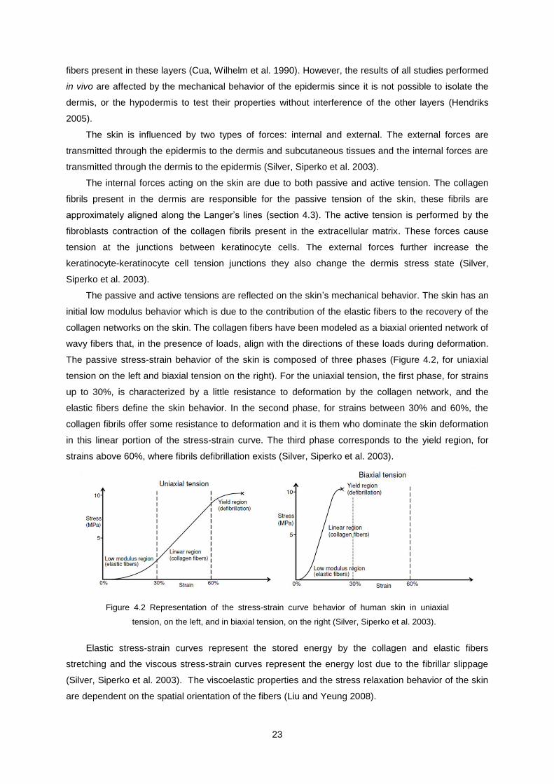
23
fibers present in these layers (Cua, Wilhelm et al. 1990). However, the results of all studies performed
in vivo are affected by the mechanical behavior of the epidermis since it is not possible to isolate the
dermis, or the hypodermis to test their properties without interference of the other layers (Hendriks
2005).
The skin is influenced by two types of forces: internal and external. The external forces are
transmitted through the epidermis to the dermis and subcutaneous tissues and the internal forces are
transmitted through the dermis to the epidermis (Silver, Siperko et al. 2003).
The internal forces acting on the skin are due to both passive and active tension. The collagen
fibrils present in the dermis are responsible for the passive tension of the skin, these fibrils are
approximately aligned along the Langer’s lines (section 4.3). The active tension is performed by the
fibroblasts contraction of the collagen fibrils present in the extracellular matrix. These forces cause
tension at the junctions between keratinocyte cells. The external forces further increase the
keratinocyte-keratinocyte cell tension junctions they also change the dermis stress state (Silver,
Siperko et al. 2003).
The passive and active tensions are reflected on the skin’s mechanical behavior. The skin has an
initial low modulus behavior which is due to the contribution of the elastic fibers to the recovery of the
collagen networks on the skin. The collagen fibers have been modeled as a biaxial oriented network of
wavy fibers that, in the presence of loads, align with the directions of these loads during deformation.
The passive stress-strain behavior of the skin is composed of three phases (Figure 4.2, for uniaxial
tension on the left and biaxial tension on the right). For the uniaxial tension, the first phase, for strains
up to 30%, is characterized by a little resistance to deformation by the collagen network, and the
elastic fibers define the skin behavior. In the second phase, for strains between 30% and 60%, the
collagen fibrils offer some resistance to deformation and it is them who dominate the skin deformation
in this linear portion of the stress-strain curve. The third phase corresponds to the yield region, for
strains above 60%, where fibrils defibrillation exists (Silver, Siperko et al. 2003).
Figure 4.2 Representation of the stress-strain curve behavior of human skin in uniaxial
tension, on the left, and in biaxial tension, on the right (Silver, Siperko et al. 2003).
Elastic stress-strain curves represent the stored energy by the collagen and elastic fibers
stretching and the viscous stress-strain curves represent the energy lost due to the fibrillar slippage
(Silver, Siperko et al. 2003). The viscoelastic properties and the stress relaxation behavior of the skin
are dependent on the spatial orientation of the fibers (Liu and Yeung 2008).
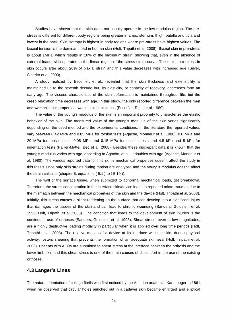
24
Studies have shown that the skin does not usually operate in the low modulus region. The pre-
stress is different for different body regions being greater in arms, sternum, thigh, patella and tibia and
lowest in the back. Skin isotropy is highest in body regions where pre-stress have highest values. The
biaxial tension is the dominant load in human skin (Holt, Tripathi et al. 2008). Biaxial skin in pre-stress
is about 1MPa, which results in 10% of the maximum strain, showing that, even in the absence of
external loads, skin operates in the linear region of the stress-strain curve. The maximum stress in
skin occurs after about 20% of biaxial strain and this value decreases with increased age (Silver,
Siperko et al. 2003).
A study realized by Escoffier, et al., revealed that the skin thickness and extensibility is
maintained up to the seventh decade but, its elasticity, or capacity of recovery, decreases form an
early age. The viscous characteristic of the skin deformation is maintained throughout life, but the
creep relaxation time decreases with age. In this study, the only reported difference between the men
and women’s skin properties, was the skin thickness (Escoffier, Rigal et al. 1989).
The value of the young’s modulus of the skin is an important propriety to characterize the elastic
behavior of the skin. The measured value of the young’s modulus of the skin varies significantly
depending on the used method and the experimental conditions. In the literature the reported values
vary between 0.42 MPa and 0.85 MPa for torsion tests (Agache, Monneur et al. 1980), 0.6 MPa and
20 MPa for tensile tests, 0.05 MPa and 0.15 MPa for suction tests and 4.5 kPa and 8 kPa for
indentation tests (Pailler-Mattei, Bec et al. 2008). Besides these discrepant data it is known that the
young’s modulus varies with age, according to Agache, et al., it doubles with age (Agache, Monneur et
al. 1980). The various reported data for this skin’s mechanical properties doesn’t affect the study in
this thesis since only skin strains during motion are analyzed and the young’s modulus doesn’t affect
the strain calculus (chapter 5, equations ( 5.1 ) to ( 5.19 )).
The wall of the surface tissue, when submitted to abnormal mechanical loads, get breakdown.
Therefore, the stress concentration in the interface skin/device leads to repeated micro-traumas due to
the mismatch between the mechanical properties of the skin and the device (Holt, Tripathi et al. 2008).
Initially, this stress causes a slight reddening on the surface that can develop into a significant injury
that damages the tissues of the skin and can lead to chronic wounding (Sanders, Goldstein et al.
1995; Holt, Tripathi et al. 2008). One condition that leads to the development of skin injuries is the
continuous use of orthoses (Sanders, Goldstein et al. 1995). Shear stress, even at low magnitudes,
are a highly destructive loading modality in particular when it is applied over long time periods (Holt,
Tripathi et al. 2008). The relative motion of a device at its interface with the skin, during physical
activity, fosters shearing that prevents the formation of an adequate skin seal (Holt, Tripathi et al.
2008). Patients with AFOs are submitted to shear stress at the interface between the orthosis and the
lower limb skin and this shear stress is one of the main causes of discomfort in the use of the existing
orthoses.
4.3 Langer’s Lines
The natural orientation of collage fibrils was first noticed by the Austrian anatomist Karl Lenger in 1861
when he observed that circular holes punched out in a cadaver skin became enlarged and elliptical
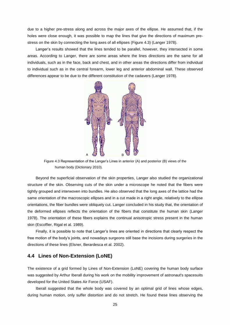
25
due to a higher pre-stress along and across the major axes of the ellipse. He assumed that, if the
holes were close enough, it was possible to map the lines that give the directions of maximum pre-
stress on the skin by connecting the long axes of all ellipses (Figure 4.3) (Langer 1978).
Langer’s results showed that the lines tended to be parallel, however, they intersected in some
areas. According to Langer, there are some areas where the lines directions are the same for all
individuals, such as in the face, back and chest, and in other areas the directions differ from individual
to individual such as in the central forearm, lower leg and anterior abdominal wall. These observed
differences appear to be due to the different constitution of the cadavers (Langer 1978).
Figure 4.3 Representation of the Langer’s Lines in anterior (A) and posterior (B) views of the
human body (Dictionary 2010).
Beyond the superficial observation of the skin properties, Langer also studied the organizational
structure of the skin. Observing cuts of the skin under a microscope he noted that the fibers were
tightly grouped and interwoven into bundles. He also observed that the long axes of the lattice had the
same orientation of the macroscopic ellipses and in a cut made in a right angle, relatively to the ellipse
orientations, the fiber bundles were obliquely cut. Langer concluded in his study that, the orientation of
the deformed ellipses reflects the orientation of the fibers that constitute the human skin (Langer
1978). The orientation of these fibers explains the continual anisotropic stress present in the human
skin (Escoffier, Rigal et al. 1989).
Finally, it is possible to note that Langer’s lines are oriented in directions that clearly respect the
free motion of the body’s joints, and nowadays surgeons still base the incisions during surgeries in the
directions of these lines (Elsner, Berardesca et al. 2002).
4.4 Lines of Non-Extension (LoNE)
The existence of a grid formed by Lines of Non-Extension (LoNE) covering the human body surface
was suggested by Arthur Iberall during his work on the mobility improvement of astronaut's spacesuits
developed for the United States Air Force (USAF).
Iberall suggested that the whole body was covered by an optimal grid of lines whose edges,
during human motion, only suffer distortion and do not stretch. He found these lines observing the
26
elastic deformation suffered by circles drawn on the human skin. During human motion, and in
agreement with the theory of elasticity, the circles drawn on the skin deform into ellipses (Iberall 1964).
He considered that the assumption of small strains was satisfactory (Iberall 1970). In some particular
cases, these ellipses have two diameters with equal length to the diameter of the initial circle. Iberall
observed that the correspondent lines to these diameters just suffer distortion during motion and do
not stretch or contract (Iberall 1964). He suggested that the directions of these LoNE, for a particular
point on the skin, correspond to the directions of interception between the original circle and the
deformed circle (ellipse) centered on that point (Figure 4.4) (Iberall 1970).
Figure 4.4 Schematic representation of the Iberall’s method to draw the directions of the
lines of non-extension (LoNE). At the left, Iberall’s LoNE for the right lower limb. At
the right, the warped circle is represented by a continuous line, the warped ellipse by
a dashed line and the LoNE by red dashed arrows (Bethke 2005).
Since the human motions are limited by their own joints, which have finite degrees of freedom (DoF),
and range of motion the experimental study realized by Iberall verified that the grid of LoNE is
essentially the same for all deformations. In practice, this finding means that the lines mapped from
extreme deformations are valid for any intermediate deformation (Iberall 1964).
The LoNE realized by Iberall were based on observation and the grid mapping was done without
relying on numerical methods indicating that the grid found by him is an approximation, with some
errors, of the lines of non-extension that exist in the body. Some of the difficulties encountered in the
line mapping were reported by Iberall himself. The lines were extended along the mapping field, a
procedure which introduced some errors, and he didn’t know how far these lines were from the real
ones. He also found lines, in critical areas, in which their angle of separation was very small, making it
difficult to get a precise direction for these lines (Iberall 1964).
To demonstrate the existence of these lines and verify their direction, Iberall drew the lines with
an inextensible cable on a man’s body and proved that there is no deformation, extension or
contraction, of the lines and there was no loss of mobility (Figure 4.5) (Iberall 1964). Iberall’s study
didn’t include the mapping of the lines of non-extension in hands and feet.
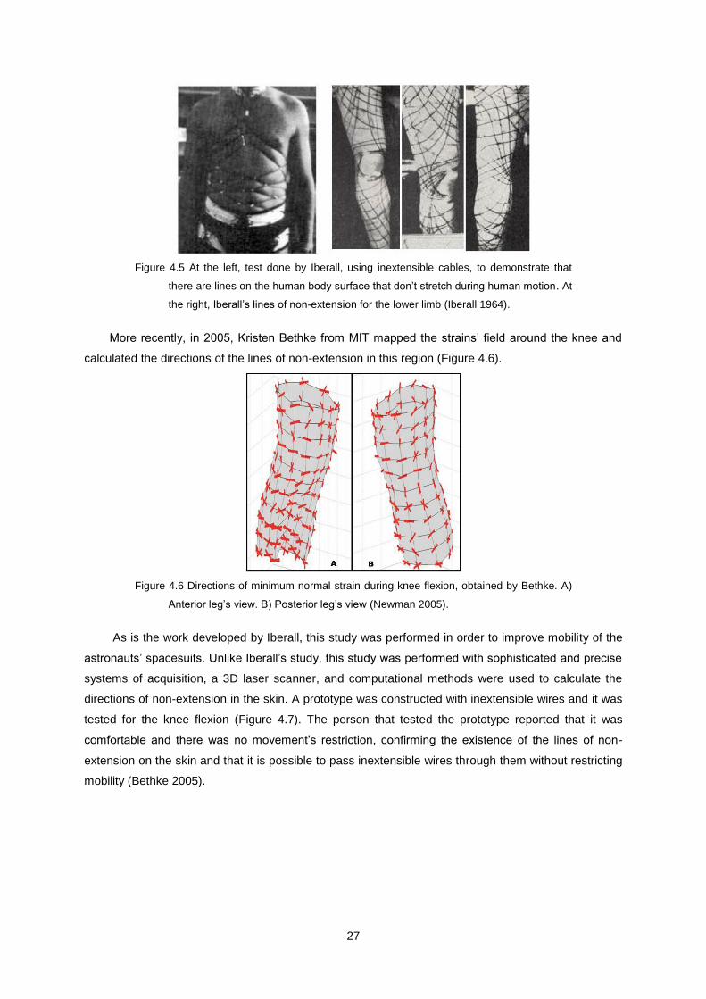
27
Figure 4.5 At the left, test done by Iberall, using inextensible cables, to demonstrate that
there are lines on the human body surface that don’t stretch during human motion. At
the right, Iberall’s lines of non-extension for the lower limb (Iberall 1964).
More recently, in 2005, Kristen Bethke from MIT mapped the strains’ field around the knee and
calculated the directions of the lines of non-extension in this region (Figure 4.6).
Figure 4.6 Directions of minimum normal strain during knee flexion, obtained by Bethke. A)
Anterior leg’s view. B) Posterior leg’s view (Newman 2005).
As is the work developed by Iberall, this study was performed in order to improve mobility of the
astronauts’ spacesuits. Unlike Iberall’s study, this study was performed with sophisticated and precise
systems of acquisition, a 3D laser scanner, and computational methods were used to calculate the
directions of non-extension in the skin. A prototype was constructed with inextensible wires and it was
tested for the knee flexion (Figure 4.7). The person that tested the prototype reported that it was
comfortable and there was no movement’s restriction, confirming the existence of the lines of non-
extension on the skin and that it is possible to pass inextensible wires through them without restricting
mobility (Bethke 2005).
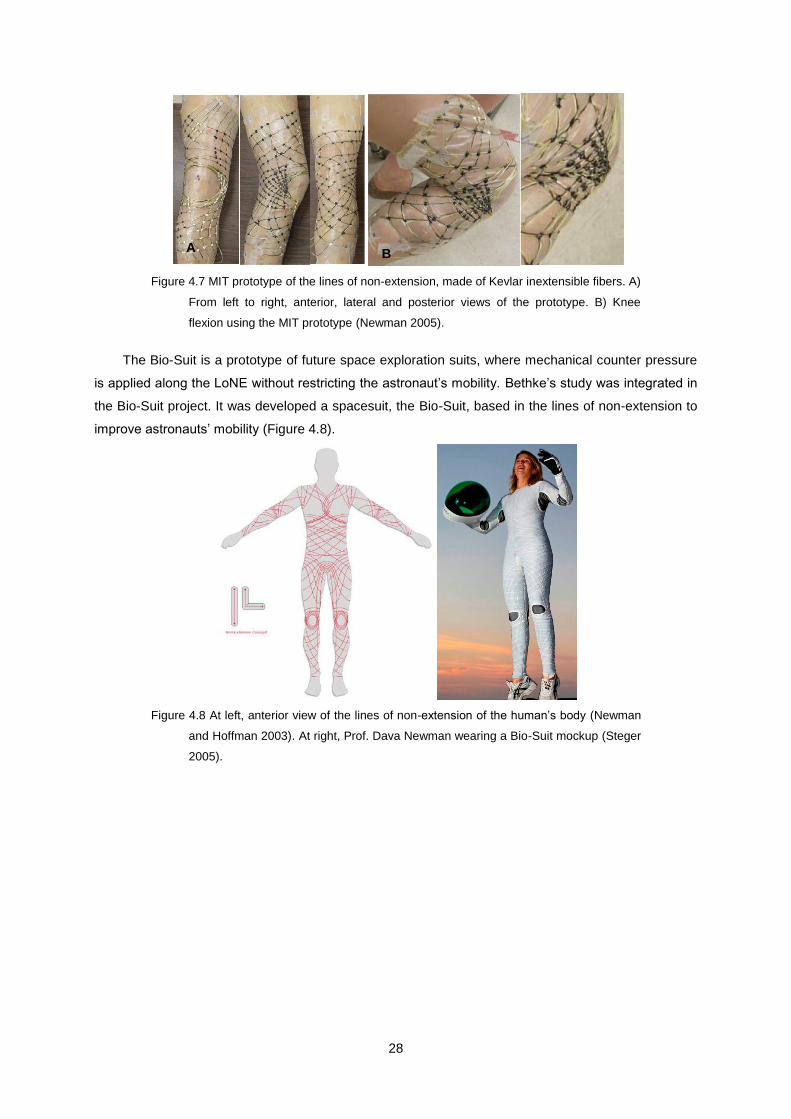
28
Figure 4.7 MIT prototype of the lines of non-extension, made of Kevlar inextensible fibers. A)
From left to right, anterior, lateral and posterior views of the prototype. B) Knee
flexion using the MIT prototype (Newman 2005).
The Bio-Suit is a prototype of future space exploration suits, where mechanical counter pressure
is applied along the LoNE without restricting the astronaut’s mobility. Bethke’s study was integrated in
the Bio-Suit project. It was developed a spacesuit, the Bio-Suit, based in the lines of non-extension to
improve astronauts’ mobility (Figure 4.8).
Figure 4.8 At left, anterior view of the lines of non-extension of the human’s body (Newman
and Hoffman 2003). At right, Prof. Dava Newman wearing a Bio-Suit mockup (Steger
2005).
A
))
B
))
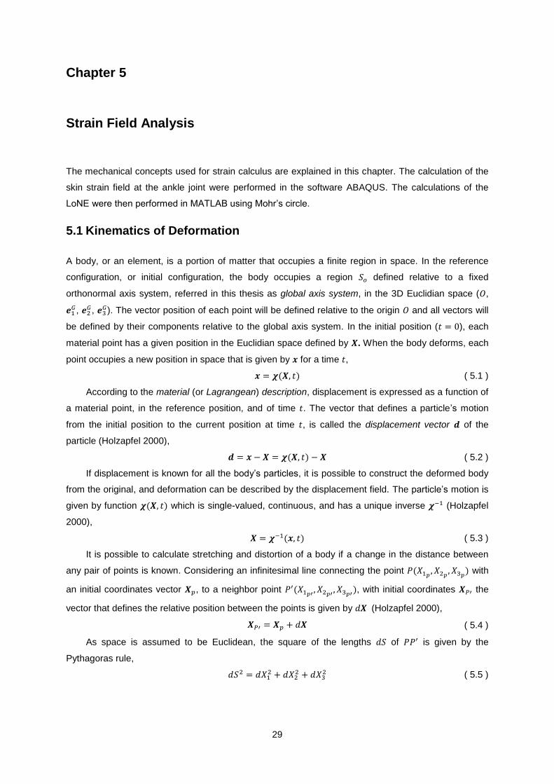
29
Chapter 5
5. Strain Field Analysis
The mechanical concepts used for strain calculus are explained in this chapter. The calculation of the
skin strain field at the ankle joint were performed in the software ABAQUS. The calculations of the
LoNE were then performed in MATLAB using Mohr’s circle.
5.1 Kinematics of Deformation
A body, or an element, is a portion of matter that occupies a finite region in space. In the reference
configuration, or initial configuration, the body occupies a region defined relative to a fixed
orthonormal axis system, referred in this thesis as global axis system, in the 3D Euclidian space ( ,
,
, ). The vector position of each point will be defined relative to the origin and all vectors will
be defined by their components relative to the global axis system. In the initial position ( ), each
material point has a given position in the Euclidian space defined by . When the body deforms, each
point occupies a new position in space that is given by for a time ,
( 5.1 )
According to the material (or Lagrangean) description, displacement is expressed as a function of
a material point, in the reference position, and of time . The vector that defines a particle’s motion
from the initial position to the current position at time , is called the displacement vector of the
particle (Holzapfel 2000),
( 5.2 )
If displacement is known for all the body’s particles, it is possible to construct the deformed body
from the original, and deformation can be described by the displacement field. The particle’s motion is
given by function which is single-valued, continuous, and has a unique inverse (Holzapfel
2000),
( 5.3 )
It is possible to calculate stretching and distortion of a body if a change in the distance between
any pair of points is known. Considering an infinitesimal line connecting the point
with
an initial coordinates vector , to a neighbor point
, with initial coordinates the
vector that defines the relative position between the points is given by (Holzapfel 2000),
( 5.4 )
As space is assumed to be Euclidean, the square of the lengths of is given by the
Pythagoras rule,
( 5.5 )
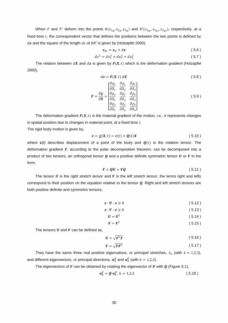
30
When and deform into the points
and
, respectively, at a
fixed time , the correspondent vector that defines the positions between the two points is defined by
and the square of the length of is given by (Holzapfel 2000).
( 5.6 )
( 5.7 )
The relation between and is given by which is the deformation gradient (Holzapfel
2000),
( 5.8 )
( 5.9 )
The deformation gradient is the material gradient of the motion, i.e., it represents changes
in spatial position due to changes in material point, at a fixed time .
The rigid body motion is given by,
( 5.10 )
where c(t) describes displacement of a point of the body and is the rotation tensor. The
deformation gradient , according to the polar decomposition theorem, can be decomposed into a
product of two tensors, an orthogonal tensor and a positive definite symmetric tensor or in the
form,
( 5.11 )
The tensor is the right stretch tensor and is the left stretch tensor, the terms right and lefts
correspond to their position on the equation relative to the tensor . Right and left stretch tensors are
both positive definite and symmetric tensors,
( 5.12 )
( 5.13 )
( 5.14 )
( 5.15 )
The tensors and can be defined as,
( 5.16 )
( 5.17 )
They have the same three real positive eigenvalues, or principal stretches, (with ),
and different eigenvectors, or principal directions, and
(with ).
The eigenvectors of can be obtained by rotating the eigenvector of with (Figure 5.1),
, ( 5.18 )
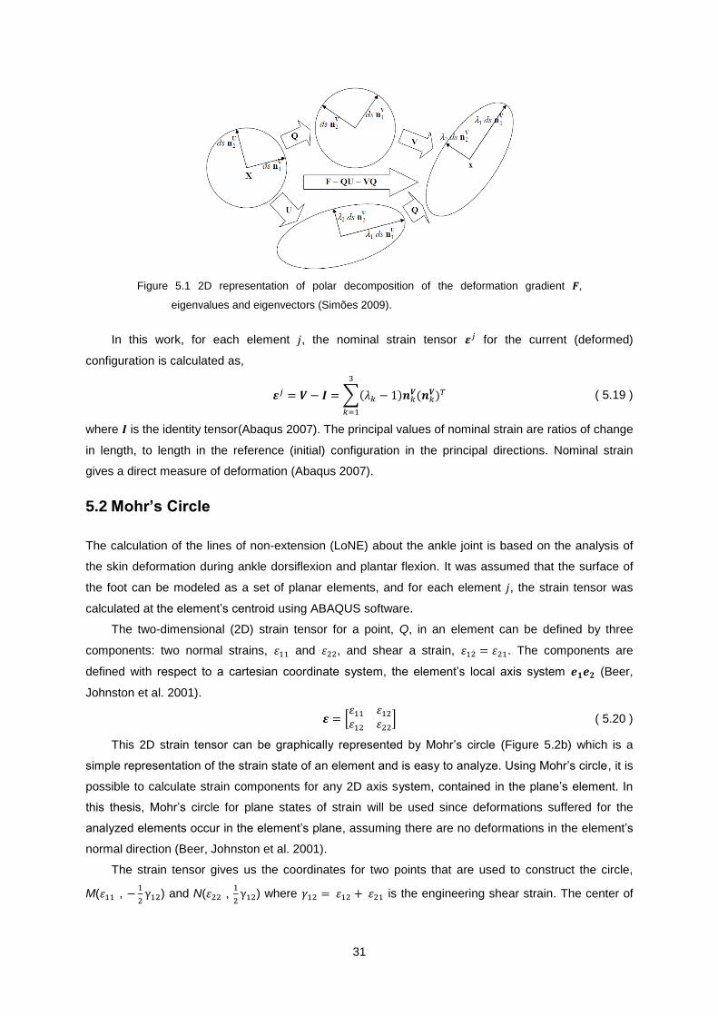
31
Figure 5.1 2D representation of polar decomposition of the deformation gradient ,
eigenvalues and eigenvectors (Simões 2009).
In this work, for each element , the nominal strain tensor for the current (deformed)
configuration is calculated as,
( 5.19 )
where is the identity tensor(Abaqus 2007). The principal values of nominal strain are ratios of change
in length, to length in the reference (initial) configuration in the principal directions. Nominal strain
gives a direct measure of deformation (Abaqus 2007).
5.2 Mohr’s Circle
The calculation of the lines of non-extension (LoNE) about the ankle joint is based on the analysis of
the skin deformation during ankle dorsiflexion and plantar flexion. It was assumed that the surface of
the foot can be modeled as a set of planar elements, and for each element , the strain tensor was
calculated at the element’s centroid using ABAQUS software.
The two-dimensional (2D) strain tensor for a point, Q, in an element can be defined by three
components: two normal strains, and , and shear a strain, . The components are
defined with respect to a cartesian coordinate system, the element’s local axis system (Beer,
Johnston et al. 2001).
( 5.20 )
This 2D strain tensor can be graphically represented by Mohr’s circle (Figure 5.2b) which is a
simple representation of the strain state of an element and is easy to analyze. Using Mohr’s circle, it is
possible to calculate strain components for any 2D axis system, contained in the plane’s element. In
this thesis, Mohr’s circle for plane states of strain will be used since deformations suffered for the
analyzed elements occur in the element’s plane, assuming there are no deformations in the element’s
normal direction (Beer, Johnston et al. 2001).
The strain tensor gives us the coordinates for two points that are used to construct the circle,
M( ,
) and N( ,
) where is the engineering shear strain. The center of
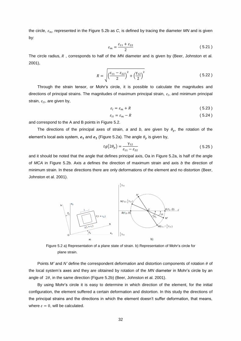
32
the circle, , represented in the Figure 5.2b as C, is defined by tracing the diameter MN and is given
by:
( 5.21 )
The circle radius, , corresponds to half of the MN diameter and is given by (Beer, Johnston et al.
2001),
( 5.22 )
Through the strain tensor, or Mohr’s circle, it is possible to calculate the magnitudes and
directions of principal strains. The magnitudes of maximum principal strain, , and minimum principal
strain, , are given by,
( 5.23 )
( 5.24 )
and correspond to the A and B points in Figure 5.2.
The directions of the principal axes of strain, a and b, are given by , the rotation of the
element’s local axis system, and (Figure 5.2a). The angle is given by,
( 5.25 )
and it should be noted that the angle that defines principal axis, Oa in Figure 5.2a, is half of the angle
of MCA in Figure 5.2b. Axis a defines the direction of maximum strain and axis b the direction of
minimum strain. In these directions there are only deformations of the element and no distortion (Beer,
Johnston et al. 2001).
Figure 5.2 a) Representation of a plane state of strain. b) Representation of Mohr’s circle for
plane strain.
Points M’ and N’ define the correspondent deformation and distortion components of rotation of
the local system’s axes and they are obtained by rotation of the MN diameter in Mohr’s circle by an
angle of , in the same direction (Figure 5.2b) (Beer, Johnston et al. 2001).
By using Mohr’s circle it is easy to determine in which direction of the element, for the initial
configuration, the element suffered a certain deformation and distortion. In this study the directions of
the principal strains and the directions in which the element doesn’t suffer deformation, that means,
where , will be calculated.

33
Chapter 6
6. Laboratory Procedure and Developed Program
In this study, data was collected from the right foot of two female subjects with 23 years old. For each
subject, the right foot was instrumented with reflectors markers covering all foot area, except the toes,
the sole, and the distal extremity of the leg. The positions of the markers, during the analyzed
movements, dorsiflexion and plantar flexion, were captured by system of four infrared cameras.
6.1 Acquisition system
The motion acquisition was performed using the Qualisys Motion Capture System, with four
ProReflexTM
MCU500 cameras (Figure 6.1). Each camera emits infrared light, which is reflected by
retro-reflective markers back to the MCU. The reflected energy from the markers is captured by the
camera’s lens where it creates a circular reproduction on the camera’s image sensor. The center and
the size of each marker is calculated in real-time, obtaining a 2D position of the marker for the axis
system of a certain camera (Qualisys 2006). The 2D image captured by each camera is used by the
Qualisys Track Manager (QTM) software to calculate the 3D spatial positions of the markers (Qualisys
2006).
The cameras were placed in the most appropriate spatial disposition, for the collection of this
study data, and calibrated. Since the laboratory only has four cameras, it was not possible to collect
360º data from the whole foot at the same time. Several spatial dispositions of the cameras were
tested and the disposition that presented less artifacts in the calculated trajectories and, at the same
time, permitted to capture the entire view of each side of the foot was chosen. The cameras were
layed out in an arc and calibrated for a small acquisition volume (Figure 6.1).
Figure 6.1 At left, disposition (in arc) of the four infrared cameras and a plastic cube
marking the acquisition volume. The picture was taken during the static calibration of
the cameras. At right, one of the infrared ProReflexTM
MCU500 cameras used in
motion capture.
To calculate the marker’s 3D spatial positions it is necessary that all markers are detected
throughout movement, at least, by two cameras. The system was tested in order to choose the most
appropriated acquisition parameters and the acquisition frequency was set to 80Hz. Although the

34
cameras have a maximum acquisition rate of 500Hz, it was not possible to use this frequency due to
the high number of markers used. Several distances between the markers were tested. With this
system, the minimum distance for correct capture using a large number of markers is 2cm.
6.2 Marker Placement
Markers were placed considering two factors: the distance between them and their spatial
organization on the skin’s surface. The study area was the skin area usually covered by a normal sock
except the toes and the foot sole. The geometric element used to analyze the skin strains was the
triangle.
The right foot of two subjects was covered with reflectors, with approximately 4mm, so that they
stay at an initial distance of approximately 2cm in the anatomical reference position of the foot, and
they were distributed in rows and columns in order to form an initial grid of squares. In the surface of
the skin’s foot located anteriorly to the ankle, it was not possible to form a grid so geometrically
aligned due to the irregular geometry of this region of the body. In this area, markers were placed in
order to form squares, whenever possible, and triangles. The principal concern of the markers
distribution in this area was to keep the distance between them approximately 2cm (Figure 6.2). Some
reference markers were also placed on the toes and leg, above the grid of markers in order to simplify
the markers identification on the QTM software.
Figure 6.2 Markers grid on the right foot’s skin of subject 1. From left to right: lateral, medial,
posterior and anterior foot’s view.
In one of the subjects, subject 1, 132 markers were placed and in the other subject, subject 2,
141 markers. The difference in the number of markers between the two subjects was due to the
difference on the diameter of the distal portion of the leg and on the foot length. Subject 1 has a lower
leg diameter (8 cm above the ankle) of 22.5 cm and a foot length, from the heel to the distal extremity
of the great toe, of 23.5 cm (Standard 1991). By contrast, subject 2 has a higher leg perimeter (8 cm
above the ankle) of 24.5 cm and a foot length (from the heel to the distal extremity of the great toe) of
25.5 cm, 37 and 40 European shoe sizes respectively.
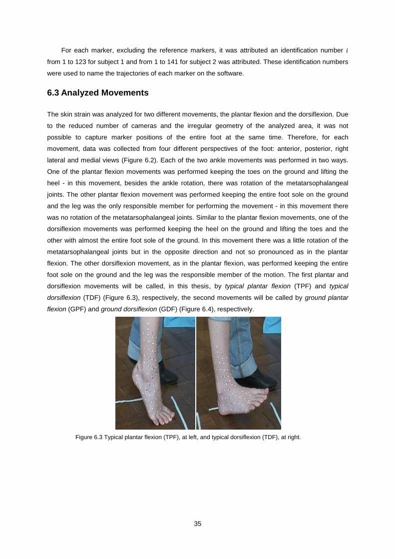
35
For each marker, excluding the reference markers, it was attributed an identification number
from 1 to 123 for subject 1 and from 1 to 141 for subject 2 was attributed. These identification numbers
were used to name the trajectories of each marker on the software.
6.3 Analyzed Movements
The skin strain was analyzed for two different movements, the plantar flexion and the dorsiflexion. Due
to the reduced number of cameras and the irregular geometry of the analyzed area, it was not
possible to capture marker positions of the entire foot at the same time. Therefore, for each
movement, data was collected from four different perspectives of the foot: anterior, posterior, right
lateral and medial views (Figure 6.2). Each of the two ankle movements was performed in two ways.
One of the plantar flexion movements was performed keeping the toes on the ground and lifting the
heel - in this movement, besides the ankle rotation, there was rotation of the metatarsophalangeal
joints. The other plantar flexion movement was performed keeping the entire foot sole on the ground
and the leg was the only responsible member for performing the movement - in this movement there
was no rotation of the metatarsophalangeal joints. Similar to the plantar flexion movements, one of the
dorsiflexion movements was performed keeping the heel on the ground and lifting the toes and the
other with almost the entire foot sole of the ground. In this movement there was a little rotation of the
metatarsophalangeal joints but in the opposite direction and not so pronounced as in the plantar
flexion. The other dorsiflexion movement, as in the plantar flexion, was performed keeping the entire
foot sole on the ground and the leg was the responsible member of the motion. The first plantar and
dorsiflexion movements will be called, in this thesis, by typical plantar flexion (TPF) and typical
dorsiflexion (TDF) (Figure 6.3), respectively, the second movements will be called by ground plantar
flexion (GPF) and ground dorsiflexion (GDF) (Figure 6.4), respectively.
Figure 6.3 Typical plantar flexion (TPF), at left, and typical dorsiflexion (TDF), at right.
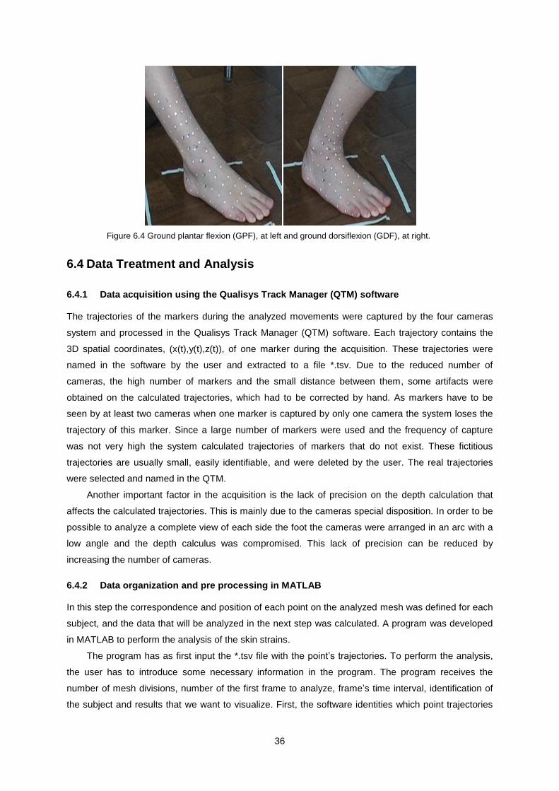
36
Figure 6.4 Ground plantar flexion (GPF), at left and ground dorsiflexion (GDF), at right.
6.4 Data Treatment and Analysis
6.4.1 Data acquisition using the Qualisys Track Manager (QTM) software
The trajectories of the markers during the analyzed movements were captured by the four cameras
system and processed in the Qualisys Track Manager (QTM) software. Each trajectory contains the
3D spatial coordinates, (x(t),y(t),z(t)), of one marker during the acquisition. These trajectories were
named in the software by the user and extracted to a file *.tsv. Due to the reduced number of
cameras, the high number of markers and the small distance between them, some artifacts were
obtained on the calculated trajectories, which had to be corrected by hand. As markers have to be
seen by at least two cameras when one marker is captured by only one camera the system loses the
trajectory of this marker. Since a large number of markers were used and the frequency of capture
was not very high the system calculated trajectories of markers that do not exist. These fictitious
trajectories are usually small, easily identifiable, and were deleted by the user. The real trajectories
were selected and named in the QTM.
Another important factor in the acquisition is the lack of precision on the depth calculation that
affects the calculated trajectories. This is mainly due to the cameras special disposition. In order to be
possible to analyze a complete view of each side the foot the cameras were arranged in an arc with a
low angle and the depth calculus was compromised. This lack of precision can be reduced by
increasing the number of cameras.
6.4.2 Data organization and pre processing in MATLAB
In this step the correspondence and position of each point on the analyzed mesh was defined for each
subject, and the data that will be analyzed in the next step was calculated. A program was developed
in MATLAB to perform the analysis of the skin strains.
The program has as first input the *.tsv file with the point’s trajectories. To perform the analysis,
the user has to introduce some necessary information in the program. The program receives the
number of mesh divisions, number of the first frame to analyze, frame’s time interval, identification of
the subject and results that we want to visualize. First, the software identities which point trajectories

37
exists in the input file, *.tsv, and builds the grid that will be analyzed. The correspondence between the
points, for each subject, was introduced in the code. It is possible to use this program to calculate the
deformation of the skin for other subjects without changing the code but the markers have to be in the
same disposition and designation of one of the analyzed subjects in this study.
The program analyses the original mesh, formed by the tracked markers, or a refined mesh,
where the number of divisions of each element edge is chosen by the user (Figure 6.5). During
refinement, the numbers to the created points are assigned and their 3D spatial position in the
different analyzed frames is calculated. In this thesis has used a refined mesh to perform the calculus
of the skin strains in order to obtain a better visualization of the line’s directions and to obtain more
precise results.
Figure 6.5 At left, original mesh. At Right, refined mesh where the edge of each element was
divided into four parts.
As in Iberall’s study, it was assumed that the deformation results for the extreme distortions are
valid for the intermediate states of distortion (Iberall 1964). The strains on the skin, during dorsiflexion
and plantar flexion, were calculated for movements from the initial position to intermediate and final
positions. Each of the two studied movements was divided into five intervals of motion. As the
movements were performed with a velocity approximately constant it was assumed that the increase
of the angle, between the dorsum and the anterior leg, was approximately constant. This assumption
means that we need to consider that the total rotation of the ankle during dorsiflexion, or plantar
flexion, corresponds to 100% of the total angle of motion. Note that, during the anatomical reference
position, it is considered that the foot is in a 0o angle.
The plantar flexion movement intervals from the anatomical reference position to the different
reached angles by the subject, were named as: 20PF, 40PF, 60PF, 80PF and 100PF. That means
that 20PF corresponds to the movement from the anatomical reference position of the foot, to 20% of
the maximum reached angle during plantar flexion and 100PF corresponds to the movement from
anatomical reference position to the maximum reached angle, 100% of the total plantar flexion
movement. As in plantar flexion the dorsiflexion intermediate movements were named based on the
angle reached in each movement. The attributed names were: 20DF, 40DF, 60DF, 80DF and 100DF.
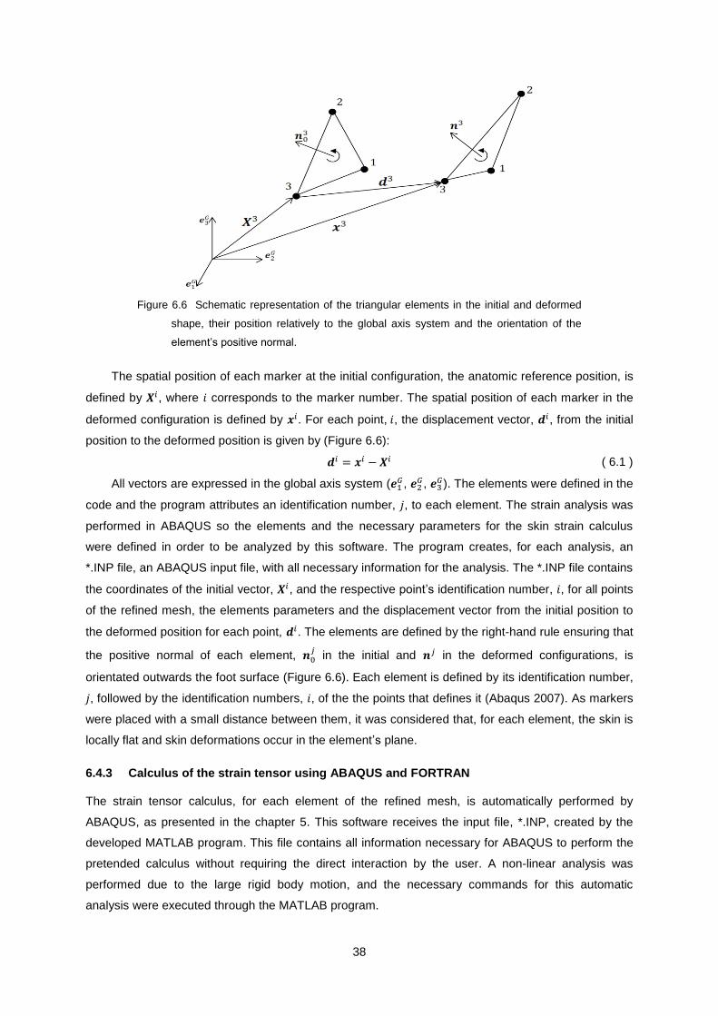
38
Figure 6.6 Schematic representation of the triangular elements in the initial and deformed
shape, their position relatively to the global axis system and the orientation of the
element’s positive normal.
The spatial position of each marker at the initial configuration, the anatomic reference position, is
defined by , where corresponds to the marker number. The spatial position of each marker in the
deformed configuration is defined by . For each point, , the displacement vector, , from the initial
position to the deformed position is given by (Figure 6.6):
( 6.1 )
All vectors are expressed in the global axis system ( ,
, ). The elements were defined in the
code and the program attributes an identification number, , to each element. The strain analysis was
performed in ABAQUS so the elements and the necessary parameters for the skin strain calculus
were defined in order to be analyzed by this software. The program creates, for each analysis, an
*.INP file, an ABAQUS input file, with all necessary information for the analysis. The *.INP file contains
the coordinates of the initial vector, , and the respective point’s identification number, , for all points
of the refined mesh, the elements parameters and the displacement vector from the initial position to
the deformed position for each point, . The elements are defined by the right-hand rule ensuring that
the positive normal of each element, in the initial and in the deformed configurations, is
orientated outwards the foot surface (Figure 6.6). Each element is defined by its identification number,
, followed by the identification numbers, , of the the points that defines it (Abaqus 2007). As markers
were placed with a small distance between them, it was considered that, for each element, the skin is
locally flat and skin deformations occur in the element’s plane.
6.4.3 Calculus of the strain tensor using ABAQUS and FORTRAN
The strain tensor calculus, for each element of the refined mesh, is automatically performed by
ABAQUS, as presented in the chapter 5. This software receives the input file, *.INP, created by the
developed MATLAB program. This file contains all information necessary for ABAQUS to perform the
pretended calculus without requiring the direct interaction by the user. A non-linear analysis was
performed due to the large rigid body motion, and the necessary commands for this automatic
analysis were executed through the MATLAB program.
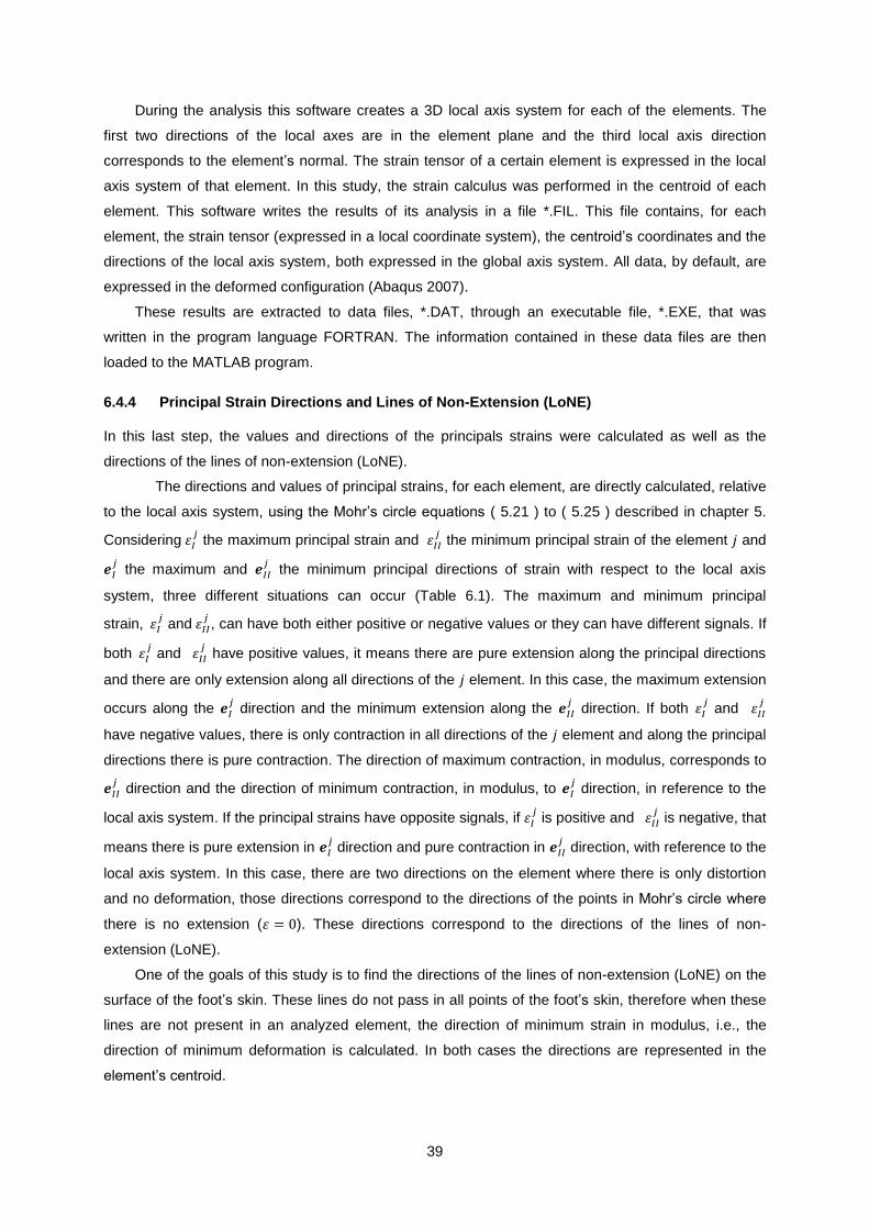
39
During the analysis this software creates a 3D local axis system for each of the elements. The
first two directions of the local axes are in the element plane and the third local axis direction
corresponds to the element’s normal. The strain tensor of a certain element is expressed in the local
axis system of that element. In this study, the strain calculus was performed in the centroid of each
element. This software writes the results of its analysis in a file *.FIL. This file contains, for each
element, the strain tensor (expressed in a local coordinate system), the centroid’s coordinates and the
directions of the local axis system, both expressed in the global axis system. All data, by default, are
expressed in the deformed configuration (Abaqus 2007).
These results are extracted to data files, *.DAT, through an executable file, *.EXE, that was
written in the program language FORTRAN. The information contained in these data files are then
loaded to the MATLAB program.
6.4.4 Principal Strain Directions and Lines of Non-Extension (LoNE)
In this last step, the values and directions of the principals strains were calculated as well as the
directions of the lines of non-extension (LoNE).
The directions and values of principal strains, for each element, are directly calculated, relative
to the local axis system, using the Mohr’s circle equations ( 5.21 ) to ( 5.25 ) described in chapter 5.
Considering the maximum principal strain and
the minimum principal strain of the element and
the maximum and
the minimum principal directions of strain with respect to the local axis
system, three different situations can occur (Table 6.1). The maximum and minimum principal
strain, and
, can have both either positive or negative values or they can have different signals. If
both and
have positive values, it means there are pure extension along the principal directions
and there are only extension along all directions of the element. In this case, the maximum extension
occurs along the direction and the minimum extension along the
direction. If both
and
have negative values, there is only contraction in all directions of the element and along the principal
directions there is pure contraction. The direction of maximum contraction, in modulus, corresponds to
direction and the direction of minimum contraction, in modulus, to direction, in reference to the
local axis system. If the principal strains have opposite signals, if is positive and
is negative, that
means there is pure extension in direction and pure contraction in
direction, with reference to the
local axis system. In this case, there are two directions on the element where there is only distortion
and no deformation, those directions correspond to the directions of the points in Mohr’s circle where
there is no extension ( ). These directions correspond to the directions of the lines of non-
extension (LoNE).
One of the goals of this study is to find the directions of the lines of non-extension (LoNE) on the
surface of the foot’s skin. These lines do not pass in all points of the foot’s skin, therefore when these
lines are not present in an analyzed element, the direction of minimum strain in modulus, i.e., the
direction of minimum deformation is calculated. In both cases the directions are represented in the
element’s centroid.
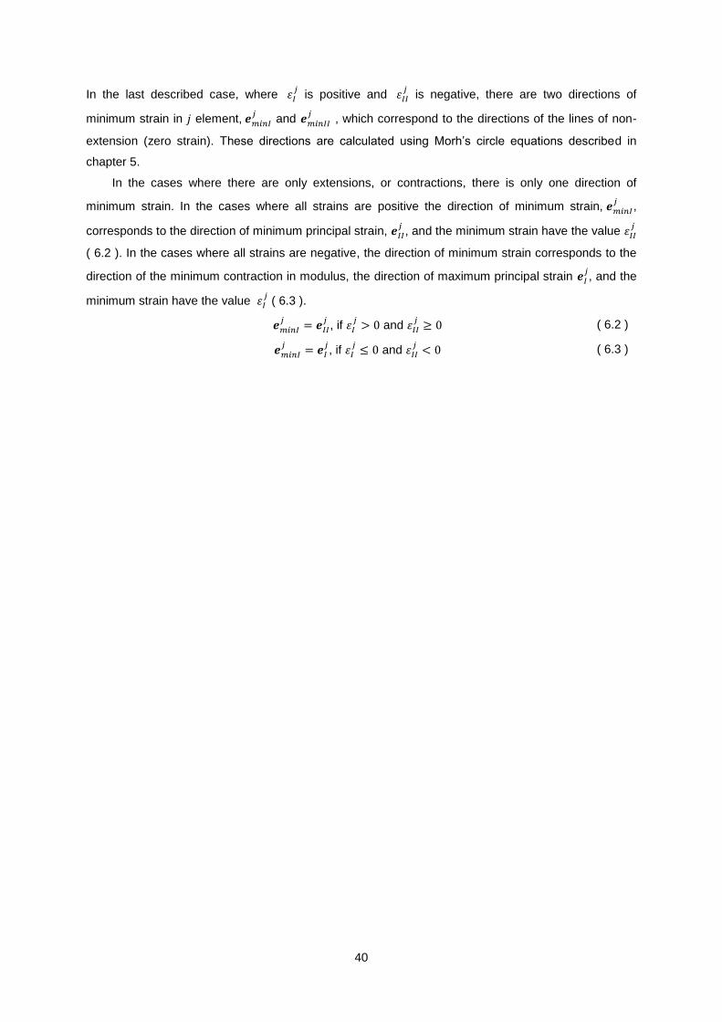
40
In the last described case, where is positive and
is negative, there are two directions of
minimum strain in element,
and
, which correspond to the directions of the lines of non-
extension (zero strain). These directions are calculated using Morh’s circle equations described in
chapter 5.
In the cases where there are only extensions, or contractions, there is only one direction of
minimum strain. In the cases where all strains are positive the direction of minimum strain,
,
corresponds to the direction of minimum principal strain,
, and the minimum strain have the value
( 6.2 ). In the cases where all strains are negative, the direction of minimum strain corresponds to the
direction of the minimum contraction in modulus, the direction of maximum principal strain , and the
minimum strain have the value ( 6.3 ).
, if and
( 6.2 )
, if
and
( 6.3 )
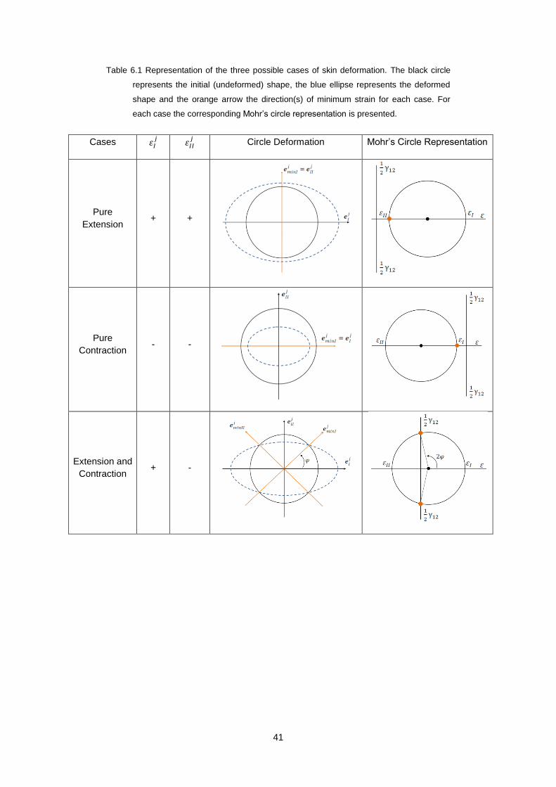
41
Table 6.1 Representation of the three possible cases of skin deformation. The black circle
represents the initial (undeformed) shape, the blue ellipse represents the deformed
shape and the orange arrow the direction(s) of minimum strain for each case. For
each case the corresponding Mohr’s circle representation is presented.
Cases
Circle Deformation Mohr’s Circle Representation
Pure
Extension + +
Pure
Contraction - -
Extension and
Contraction + -

42
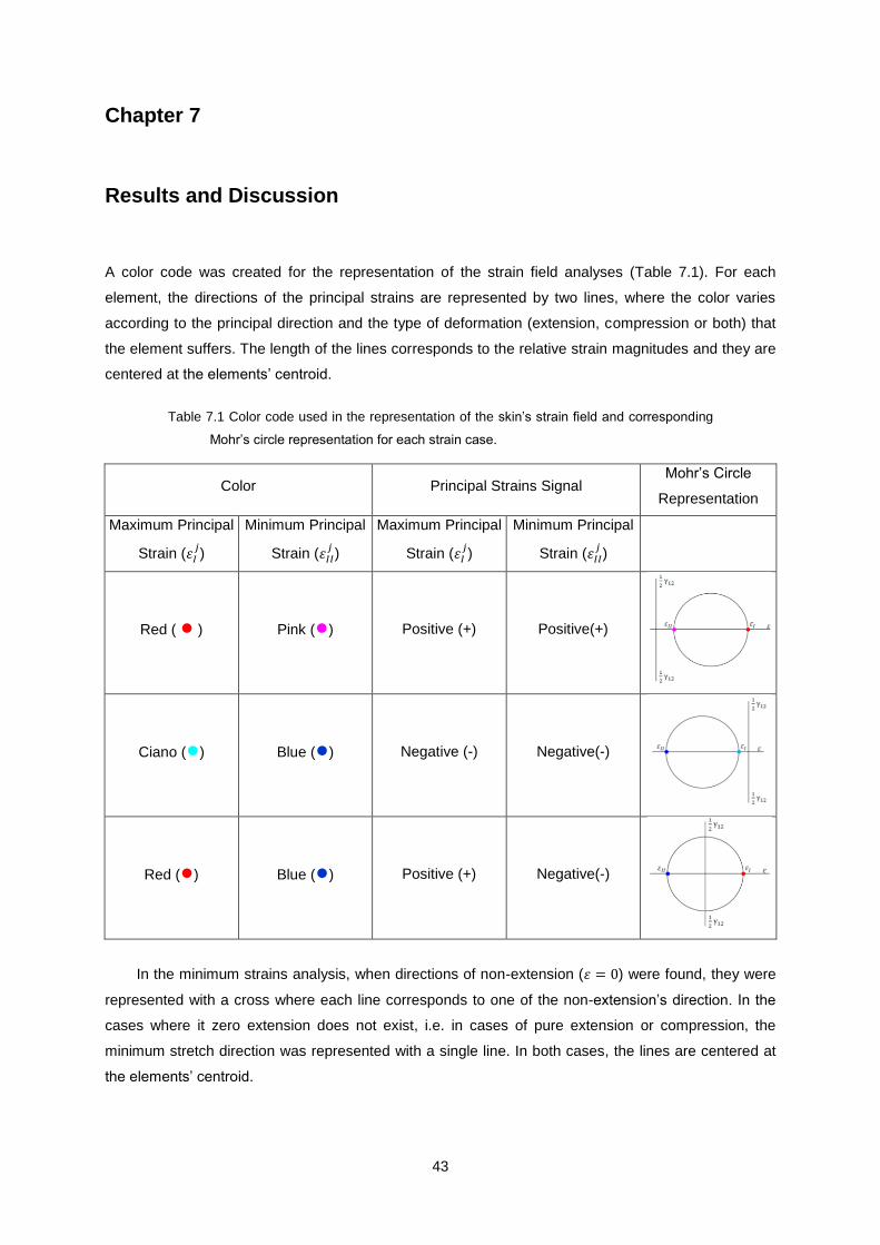
43
Chapter 7
7. Results and Discussion
A color code was created for the representation of the strain field analyses (Table 7.1). For each
element, the directions of the principal strains are represented by two lines, where the color varies
according to the principal direction and the type of deformation (extension, compression or both) that
the element suffers. The length of the lines corresponds to the relative strain magnitudes and they are
centered at the elements’ centroid.
Table 7.1 Color code used in the representation of the skin’s strain field and corresponding
Mohr’s circle representation for each strain case.
Color Principal Strains Signal Mohr’s Circle
Representation
Maximum Principal
Strain ( )
Minimum Principal
Strain ( )
Maximum Principal
Strain ( )
Minimum Principal
Strain ( )
Red ( ● ) Pink (●) Positive (+) Positive(+)
Ciano (●) Blue (●) Negative (-) Negative(-)
Red (●) Blue (●) Positive (+) Negative(-)
In the minimum strains analysis, when directions of non-extension ( ) were found, they were
represented with a cross where each line corresponds to one of the non-extension’s direction. In the
cases where it zero extension does not exist, i.e. in cases of pure extension or compression, the
minimum stretch direction was represented with a single line. In both cases, the lines are centered at
the elements’ centroid.

44
To simplify the description of the foot’s lines and strain directions, we will call longitudinal
direction to a proximal to distal direction on the skin and circumferential direction the direction radial to
longitudinal (Figure 7.1).
Figure 7.1 Representation of the longitudinal and circumferential directions on the foot. The
red lines represent the directions defined as longitudinal and the green lines the
directions defined as circumferential (adapted from (Winandy 2009)).
As it was referred in chapter 6, all analyses are from the right foot and it wasn’t possible to
analyze all the foot surface at the same time, so the results for each movement will be presented in
different views of the foot. The original mesh (not refined) difficult the strain field analysis due to the
low amount of information (Figure 7.2) so a refined mesh was used (each triangle was divided into 16
triangles), for each of the different analyses.
Figure 7.2 At left, principal strains’ field for the typical plantar flexion (TPF) represented in
the deformed configuration 100PF. At right, the directions of minimum strain. Both
analyses were performed with the original mesh (not refined), in the right lateral view
and yellow diamond indicates the lateral malleolus location.
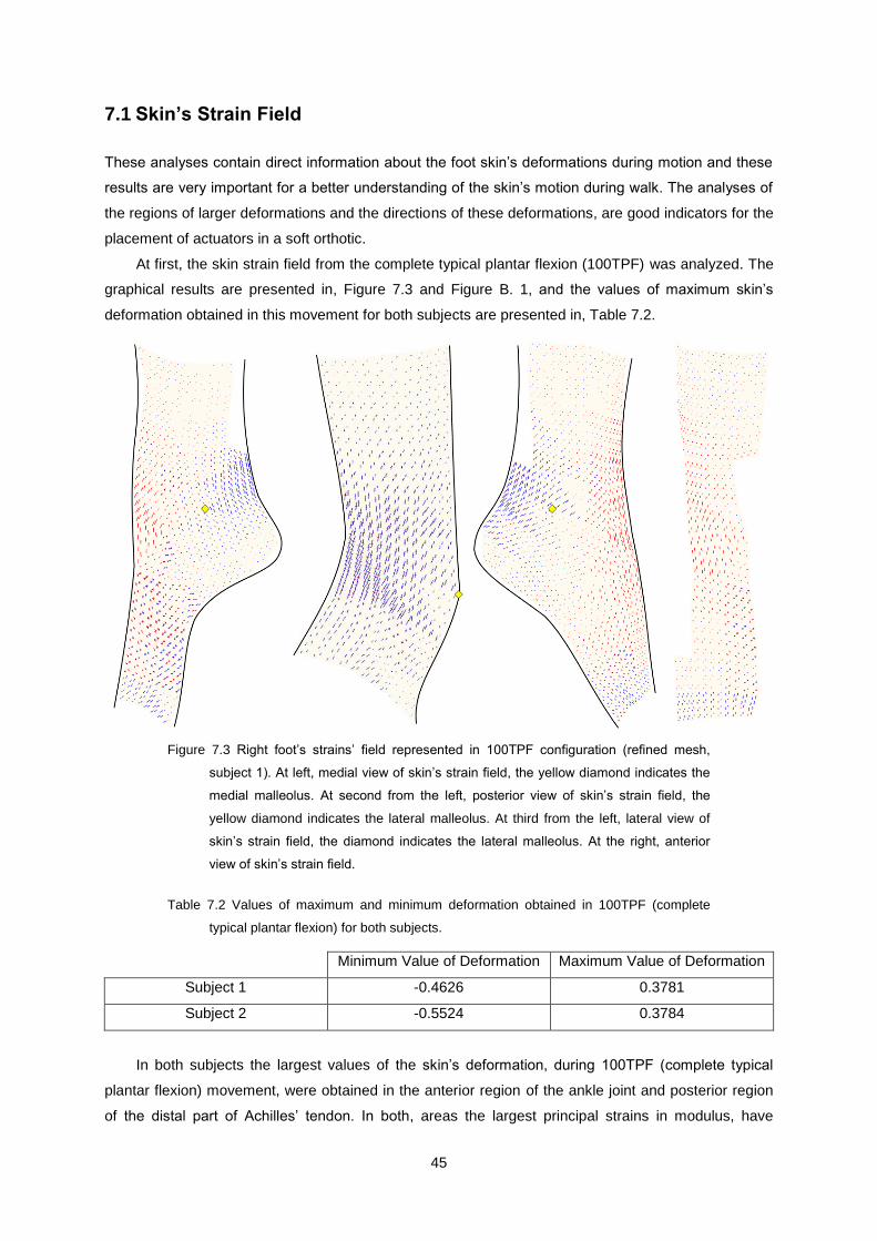
45
7.1 Skin’s Strain Field
These analyses contain direct information about the foot skin’s deformations during motion and these
results are very important for a better understanding of the skin’s motion during walk. The analyses of
the regions of larger deformations and the directions of these deformations, are good indicators for the
placement of actuators in a soft orthotic.
At first, the skin strain field from the complete typical plantar flexion (100TPF) was analyzed. The
graphical results are presented in, Figure 7.3 and Figure B. 1, and the values of maximum skin’s
deformation obtained in this movement for both subjects are presented in, Table 7.2.
Figure 7.3 Right foot’s strains’ field represented in 100TPF configuration (refined mesh,
subject 1). At left, medial view of skin’s strain field, the yellow diamond indicates the
medial malleolus. At second from the left, posterior view of skin’s strain field, the
yellow diamond indicates the lateral malleolus. At third from the left, lateral view of
skin’s strain field, the diamond indicates the lateral malleolus. At the right, anterior
view of skin’s strain field.
Table 7.2 Values of maximum and minimum deformation obtained in 100TPF (complete
typical plantar flexion) for both subjects.
Minimum Value of Deformation Maximum Value of Deformation
Subject 1 -0.4626 0.3781
Subject 2 -0.5524 0.3784
In both subjects the largest values of the skin’s deformation, during 100TPF (complete typical
plantar flexion) movement, were obtained in the anterior region of the ankle joint and posterior region
of the distal part of Achilles’ tendon. In both, areas the largest principal strains in modulus, have
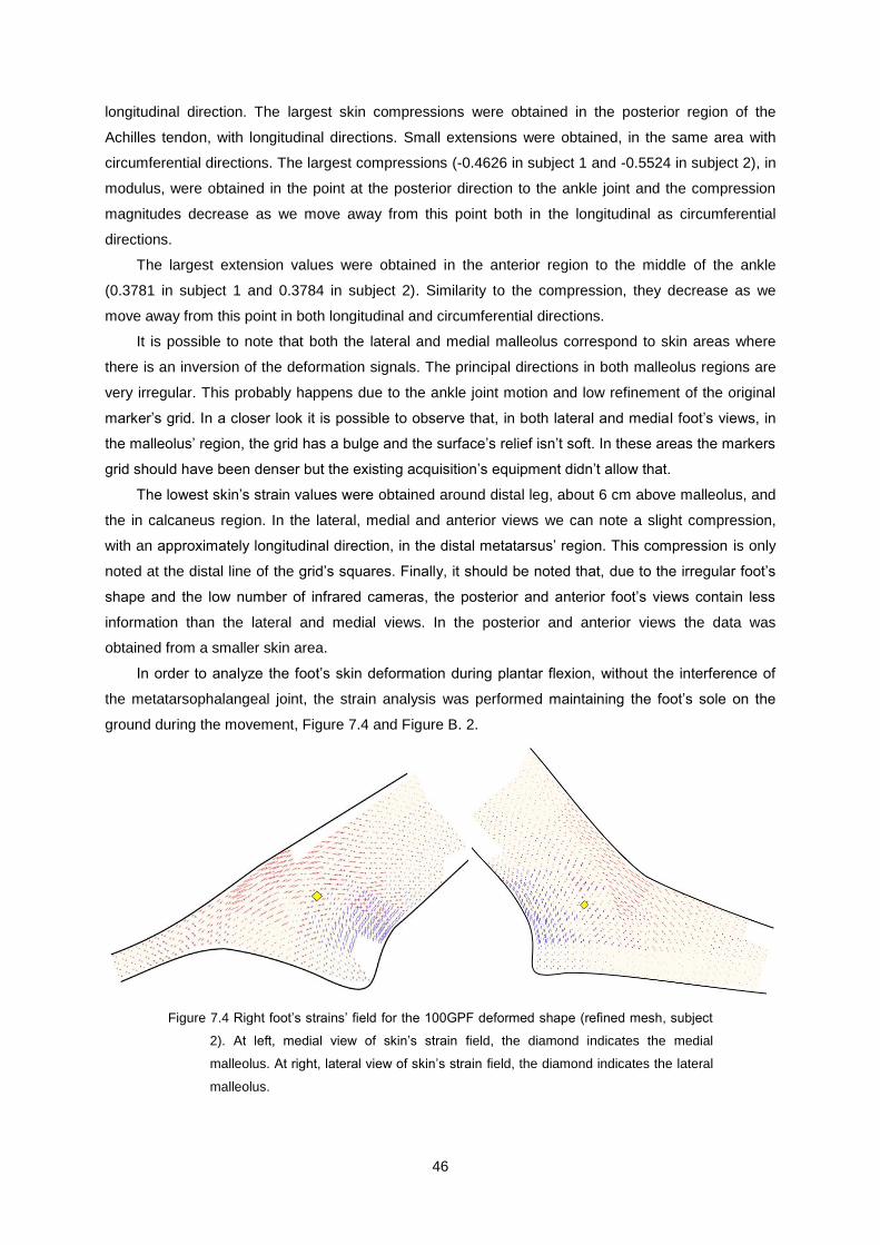
46
longitudinal direction. The largest skin compressions were obtained in the posterior region of the
Achilles tendon, with longitudinal directions. Small extensions were obtained, in the same area with
circumferential directions. The largest compressions (-0.4626 in subject 1 and -0.5524 in subject 2), in
modulus, were obtained in the point at the posterior direction to the ankle joint and the compression
magnitudes decrease as we move away from this point both in the longitudinal as circumferential
directions.
The largest extension values were obtained in the anterior region to the middle of the ankle
(0.3781 in subject 1 and 0.3784 in subject 2). Similarity to the compression, they decrease as we
move away from this point in both longitudinal and circumferential directions.
It is possible to note that both the lateral and medial malleolus correspond to skin areas where
there is an inversion of the deformation signals. The principal directions in both malleolus regions are
very irregular. This probably happens due to the ankle joint motion and low refinement of the original
marker’s grid. In a closer look it is possible to observe that, in both lateral and medial foot’s views, in
the malleolus’ region, the grid has a bulge and the surface’s relief isn’t soft. In these areas the markers
grid should have been denser but the existing acquisition’s equipment didn’t allow that.
The lowest skin’s strain values were obtained around distal leg, about 6 cm above malleolus, and
the in calcaneus region. In the lateral, medial and anterior views we can note a slight compression,
with an approximately longitudinal direction, in the distal metatarsus’ region. This compression is only
noted at the distal line of the grid’s squares. Finally, it should be noted that, due to the irregular foot’s
shape and the low number of infrared cameras, the posterior and anterior foot’s views contain less
information than the lateral and medial views. In the posterior and anterior views the data was
obtained from a smaller skin area.
In order to analyze the foot’s skin deformation during plantar flexion, without the interference of
the metatarsophalangeal joint, the strain analysis was performed maintaining the foot’s sole on the
ground during the movement, Figure 7.4 and Figure B. 2.
Figure 7.4 Right foot’s strains’ field for the 100GPF deformed shape (refined mesh, subject
2). At left, medial view of skin’s strain field, the diamond indicates the medial
malleolus. At right, lateral view of skin’s strain field, the diamond indicates the lateral
malleolus.

47
Observing the strain’s field from the 100GPF (total ground plantar flexion, Figure 7.4) is possible
to note that the relative magnitudes and directions of the skin’s principal strains are approximately
equal to the obtained in 100TPF except in the distal metatarsus’ region. In the 100GPF, the slight
compression verified in the distal metatarsus’ region at 100TPF is not present. In the ground
movement, there is no interference of the metatarsophalangeal joint in the skin’s deformation, unlike
the case of the typical plantar flexion.
The skin strain field from the complete typical dorsiflexion (100TDF) is presented in Figure 7.5
and Figure B. 3, and the values of maximum skin’s deformation for both subjects in Table 7.3.
Figure 7.5 Right foot’s strains’ field represented in 100TDF (complete typical dorsiflexion,
subject 1). At left, medial view of skin’s strain field, the yellow diamond indicates the
medial malleolus. At right, lateral view of skin’s strain field, the diamond indicates the
lateral malleolus.
Table 7.3 Values of maximum and minimum deformation obtained in 100TDF (complete
typical dorsiflexion) for both subjects.
Minimum Value of Deformation Maximum Value of Deformation
Subject 1 -0.2068 0.2593
Subject 2 -0.3421 0.2679
As in the previous analyses, the largest values of skin’s deformations were obtained in the
anterior region to ankle joint and in the posterior region to the Achilles’ tendon. In the 100TDF
(complete typical dorsiflexion) strains’ analyses the largest strains have a longitudinal direction like in
100TPF but with opposite signals. In dorsiflexion, the largest skin’s compression (-0.2068 in subject 1
and -0.3421 in subject 2) take place in the anterior region to ankle joint and the largest skin’s
extension (0.2593 in subject 1 and 0.2679 subject 2) occur in the posterior region to the distal portion
of Achilles’ tendon. When comparing the maximum strain’s values that were obtained in the 100TDF
analyses with the correspondent values in 100TPF, the magnitudes were smaller in this analysis.
Dorsiflexion is a less broad movement than plantar flexion so the total skin’s deformation is smaller.
48
In the dorsiflexion movement, as in plantar flexion, the lowest skin’s strains values, in modulus,
were obtained in the calcaneus region and around the distal leg, about 6cm above malleolus.
In this analysis it was also observed that, on both malleolus regions the marker’s grid wasn’t suitably
refined and the data from this region don’t contain enough information to perform a detailed analysis of
the skin’s deformation in this region.
Finally, in this movement, unlike what happens in 100TPF, the metatarsophalangeal joint doesn’t
seem to influence the skin’s deformation during dorsiflexion.
7.2 Directions of Minimum Skin Stretch
The minimum skin’s strains directions were graphically represented in the foot’s anatomical reference
position. The representation in this configuration allows a simplified perception and analysis of these
directions. As the developed program represents the results in the deformed shape, these analyses
were performed considering the initial configuration the total plantar flexion position, or total
dorsiflexion position, and the deformed configuration the anatomical reference position. This change
doesn’t affect the results because, as it was explained in chapter 5, the motion function has a unique
inverse so, despite the principals strains’ signals being opposite to the direct analysis, the directions of
minimum strains for each element, are the same.
We first present the directions of minimum strain for the complete typical plantar flexion
movement (100TPF), Figure 7.6 and Figure B. 4.
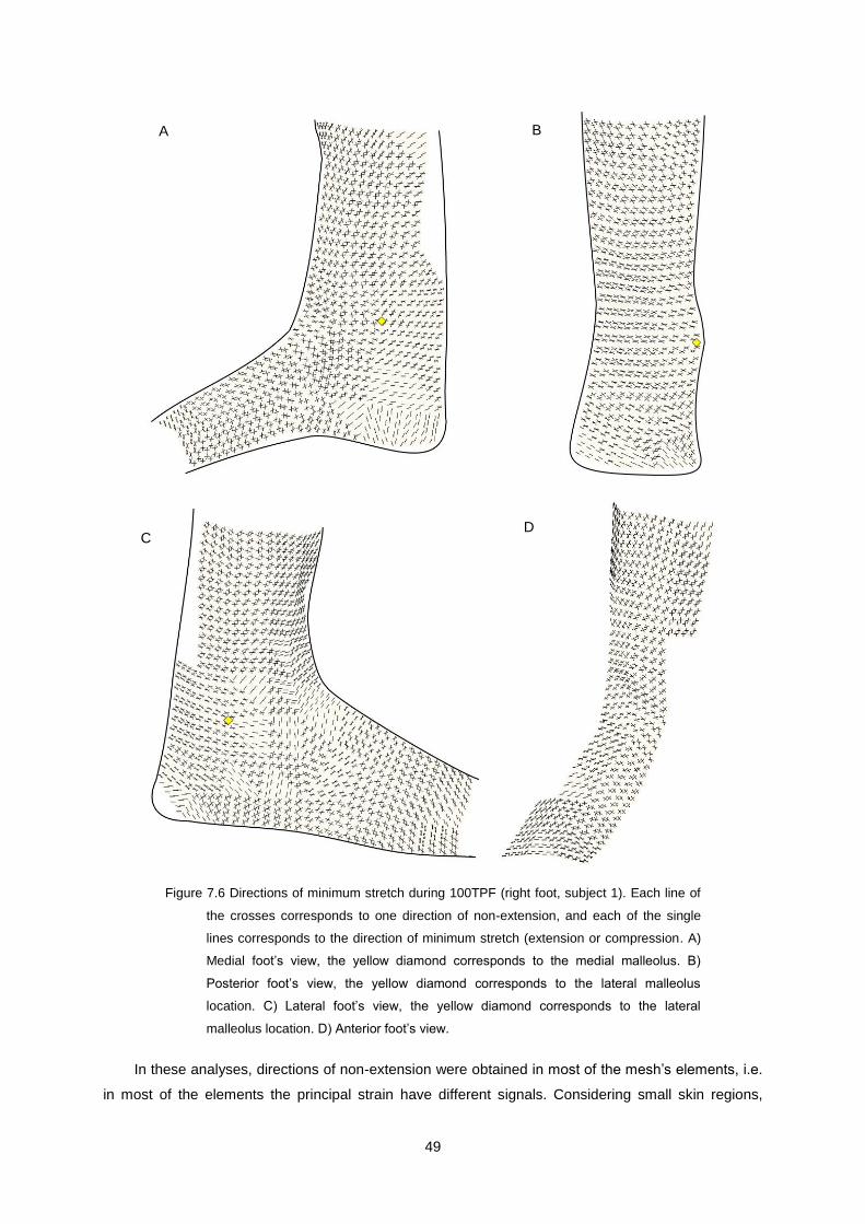
49
Figure 7.6 Directions of minimum stretch during 100TPF (right foot, subject 1). Each line of
the crosses corresponds to one direction of non-extension, and each of the single
lines corresponds to the direction of minimum stretch (extension or compression. A)
Medial foot’s view, the yellow diamond corresponds to the medial malleolus. B)
Posterior foot’s view, the yellow diamond corresponds to the lateral malleolus
location. C) Lateral foot’s view, the yellow diamond corresponds to the lateral
malleolus location. D) Anterior foot’s view.
In these analyses, directions of non-extension were obtained in most of the mesh’s elements, i.e.
in most of the elements the principal strain have different signals. Considering small skin regions,
A B
C D

50
these results shows that, during this movement, the skin adapts to the foot’s movement compressing
in one direction and extending in the other. In these cases of strain, as explained in chapter 6, two
directions where skin only suffers distortion exist and doesn’t suffer deformation (zero deformation).
In these results three skin regions were obtained, where the directions of minimum strain, in all
surface’s elements, are perfectly consistent between them (Table 7.4).
Table 7.4 Foot and leg regions where the directions of minimum strain are perfectly
consistent between the elements. Identification, illustration and respective anatomical
description of the skin’s regions. Analyses from typical plantar flexion, subject 1.
Region’s
Identification
Illustration of the Anatomical
Location Description of the Anatomical Location
R1
Distal leg’s and foot’s skin with a posterior
location to both lateral and medial malleolus
and a superior location of 2 cm bellow the
ankle joint.
R2
Between the proximal extremity of
metatarsals and 2 cm proximally to their
distal end.
R3
Distal leg’s skin with an anterior position to
both lateral and medial malleolus and a
superior location of 2cm above the ankle
joint.
In these three regions all the directions of minimum strain are directions of non-extension. The
transition between these directions is soft from an element to the adjacent element, i.e. following the
directions of minimum extension is easy to note the skin’s orientation of the lines of non-extension
(LoNE) in these regions.
On the remaining skin surface of the foot and leg, some inconsistencies were obtained in the
directions of minimum stretch between the elements of the initial mesh. In some cases, in the
transition between two adjacent elements, the line’s directions are not perfectly aligned and these
inconsistencies were verified more often in three distinct regions (Table 7.5).

51
Table 7.5 Foot and leg regions where the directions of minimum strain have some
inconsistencies between the elements of the original mesh. Identification, illustration
and anatomical description of the skin’s regions. Analyses from typical plantar
flexion, subject 1.
Region’s
Identification
Illustration of the Anatomical
Location Description of the Anatomical Location
R4
Between the distal extremity of metatarsals
and 2cm proximally to this extremity.
R5
Calcaneus region. Foot’s skin with a posterior
location to both lateral and medial malleolus
and 2 cm bellow the ankle joint.
R6
Between the proximal extremity of
metatarsals, the anterior region to both lateral
and medial malleolus and bellow 2 cm above
the ankle joint.
In these three regions some differences exist in the cause and type of the obtained
inconsistencies. In region R4, the skin suffers direct influence of the metatarsophalangeal joint, during
the analyzed movement (typical plantar flexion). This influence was already observed in the principal
strain’s field results, where, like in these results, exists a discontinuity between the foot’s distal line of
original squares elements and the adjacent elements. The calcaneus region, region R5, is formed by
two lines of squares from the original mesh. In some triangles of the proximal line consistence is
verified with the results of the adjacent triangles in region R1, but in the distal line of squares results
were obtained that are inconsistent when compared with the adjacent surface results. In this region,
the lowest values of principal strain were obtained, in modulus, and in most of the triangles directions
of non-extension were not found.
There are two possible causes for these results in R4, the markers trajectories’ noise and the
influence of body weight when the heel is on the ground. As in this region the skin’s deformation is low
the markers trajectories’ noise has a larger influence in the calculus of the directions of minimum
strain, introducing some errors in these directions. This movement begins with the foot in the
anatomical reference position so heel’s skin suffers a slight compression due to the foot standing on
the ground and this compression, in addition to the larger influence of the trajectories’ noise, in this
region, results in a region where the calculated directions of minimum strain are inconsistent between
them.

52
The region R6 is a region where interesting results were obtained. In the anterior ankle region, it
high extension values were obtained with aligned directions between the mesh elements in all foot
views. However, for the minimum stretch results, there are some differences between these views. In
the lateral foot view the elements of the original mesh form some triangles, obtaining for those
elements just one direction of minimum strain, whereas in the others two directions were obtained but
with a small angle between them. These results are a little different from those obtained in the anterior
and medial view where we obtained, in all elements, two directions of minimum strain (non-extension)
for the same region. Despite the differences in the orientation of the lines between the analyzed views,
they are consistent. Analyzing the sequence of results from the same movement (20TPF, 40TPF,
60TPF, 80TPF and 100TPF) for the lateral view, it is possible to notice that, in the lateral view, for less
broad movements two directions of non-extension were obtained As the amplitude of the movement
increases the, angle between the lines decreases until they become just one line (Appendix A). The
obtained differences between the lateral view and the other two views can be the reflex of the noise in
the calculated trajectories. A small angle between the two directions of non-extension means that one
of the principal strains is near to zero and if exists noise in the trajectory, even small, it can be enough
to change the signal of this principal strain and change the type of results (non-zero minimum strain or
two directions of non-extension).
In both medial and lateral foot views, in the regions of the transverses arches and the regions
with an anterior position to both malleolus corresponds to the foot’s regions where the low refinement
of the original mesh is more visible. Like in the anterior region to the ankle joint, elements were
obtained with just one direction of minimum strain. The transition between the obtained directions isn’t
soft and the triangles that form the original mesh (not refined) are perfectly identifiable, contrasting to
the results obtained in the regions R1, R2 and R3. Despite the obtained inconsistencies, and looking
to the entire regions, and not just from an element to the adjacent elements, it is possible to find some
directions where lines of non-extension clearly pass. Some of the obtained directions in one element,
from the original mesh, don’t have a soft continuity with the directions of the adjacent elements but
have continuity with one a little further. These regions are the most irregular in the foot and the ones
where more problems to calculate the markers trajectories were found because they weren’t always
caught by the cameras. In these regions both malleolus have a large influence in the skin’s
deformation and the markers grid didn’t have enough density of markers to accurately capture the
skin’s deformations. This low markers density of the original mesh is perfectly visible in the malleolus
region where the mesh makes a peak.
The directions of minimum strain were also calculated for the typical dorsiflexion movement,
Figure 7.7 and Figure B. 5.
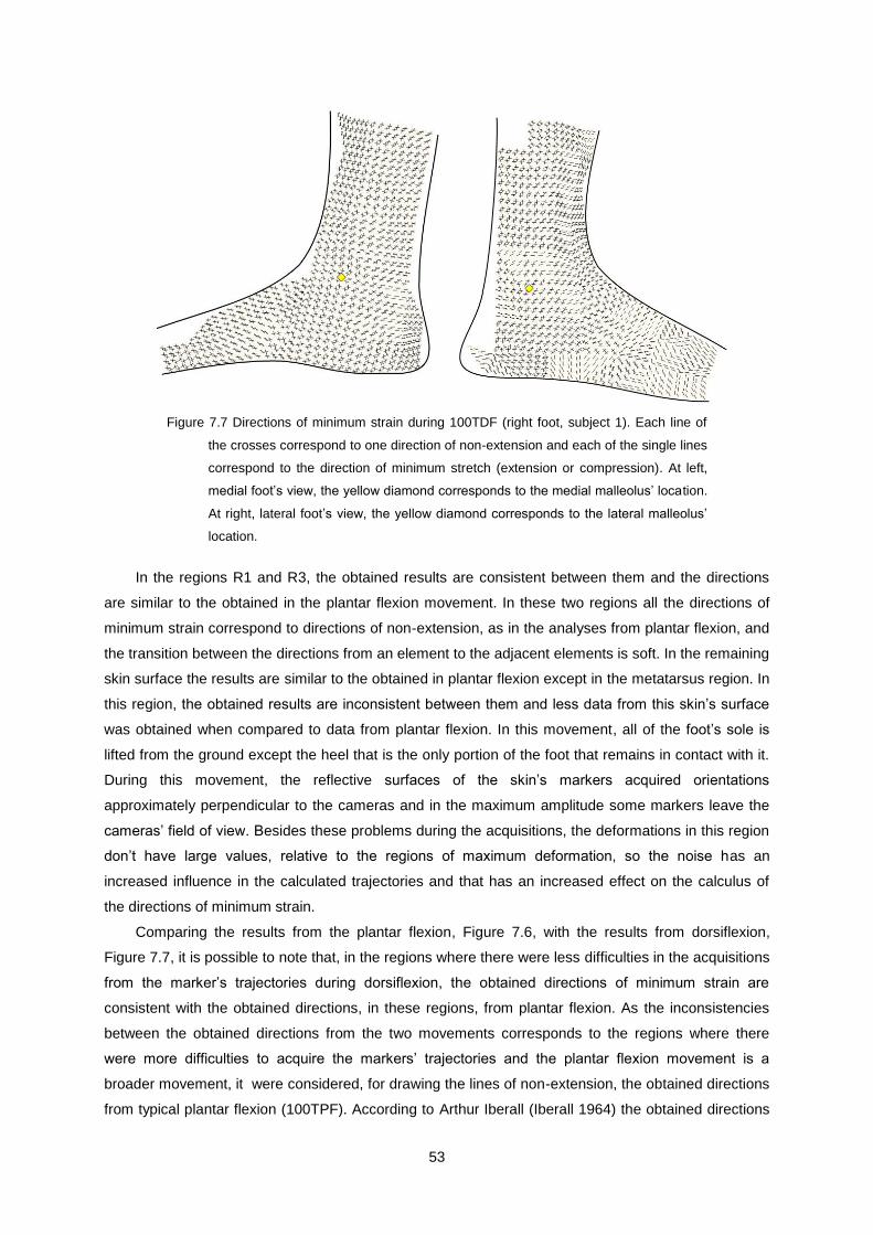
53
Figure 7.7 Directions of minimum strain during 100TDF (right foot, subject 1). Each line of
the crosses correspond to one direction of non-extension and each of the single lines
correspond to the direction of minimum stretch (extension or compression). At left,
medial foot’s view, the yellow diamond corresponds to the medial malleolus’ location.
At right, lateral foot’s view, the yellow diamond corresponds to the lateral malleolus’
location.
In the regions R1 and R3, the obtained results are consistent between them and the directions
are similar to the obtained in the plantar flexion movement. In these two regions all the directions of
minimum strain correspond to directions of non-extension, as in the analyses from plantar flexion, and
the transition between the directions from an element to the adjacent elements is soft. In the remaining
skin surface the results are similar to the obtained in plantar flexion except in the metatarsus region. In
this region, the obtained results are inconsistent between them and less data from this skin’s surface
was obtained when compared to data from plantar flexion. In this movement, all of the foot’s sole is
lifted from the ground except the heel that is the only portion of the foot that remains in contact with it.
During this movement, the reflective surfaces of the skin’s markers acquired orientations
approximately perpendicular to the cameras and in the maximum amplitude some markers leave the
cameras’ field of view. Besides these problems during the acquisitions, the deformations in this region
don’t have large values, relative to the regions of maximum deformation, so the noise has an
increased influence in the calculated trajectories and that has an increased effect on the calculus of
the directions of minimum strain.
Comparing the results from the plantar flexion, Figure 7.6, with the results from dorsiflexion,
Figure 7.7, it is possible to note that, in the regions where there were less difficulties in the acquisitions
from the marker’s trajectories during dorsiflexion, the obtained directions of minimum strain are
consistent with the obtained directions, in these regions, from plantar flexion. As the inconsistencies
between the obtained directions from the two movements corresponds to the regions where there
were more difficulties to acquire the markers’ trajectories and the plantar flexion movement is a
broader movement, it were considered, for drawing the lines of non-extension, the obtained directions
from typical plantar flexion (100TPF). According to Arthur Iberall (Iberall 1964) the obtained directions
54
of non-extension from an extreme skin’s deformation are valid for the intermediates deformations and
as the results from the skin’s surface where there were no problems during the acquisitions are
consistent to the correspondent directions from plantar flexion it was assumed that the obtained LoNE
from plantar flexion are valid for the dorsiflexion.
7.3 Lines of Non-Extension
The obtained directions of minimum strain, in sub-chapter 7.2, for punctual locations on the foot and
leg give the information to estimate the location and orientation of the lines of non-extension (LoNE) in
the analyzed anatomical region. The lines were drawn by hand and it was taken into account a series
of information and presuppositions during the drawing.
The LoNE were drawn based on the results of the minimum strains’ field from typical plantar
flexion (100TPF) and it was assumed that these lines are valid for the dorsiflexion movement, as it
was explained in the last sub-chapter. Despite the directions of non-extension in the malleolus regions
that were found, the lines drawn pass around these regions, giving to this area more freedom in the
movement. For the drawing of the LoNE, not just the directions of minimum strain were taken into
account but also the information of the principal’s strain field. The orientation of the lines was drawn
following parallel directions to the punctual minimum strain directions. In the cases where it was found
inconsistencies between the directions, the obtained directions in more distant elements was taken in
consideration from the critical points and the information from the principal strains’ field (the direction
of minimum strain can’t be parallel to the direction of maximum strain, in modulus).
Seven sets of lines of non-extension (LoNE) with parallel orientations were obtained (Table 7.6).
Each set of lines was drawn with a different color for a better visualization.
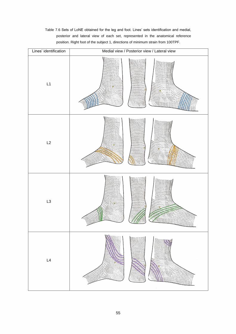
55
Table 7.6 Sets of LoNE obtained for the leg and foot. Lines’ sets identification and medial,
posterior and lateral view of each set, represented in the anatomical reference
position. Right foot of the subject 1, directions of minimum strain from 100TPF.
Lines’ identification Medial view / Posterior view / Lateral view
L1
L2
L3
L4

56
Table 7.6 Sets of LoNE obtained for the leg and foot (continuation).
L5
L6
L7
The description of the lines location is performed for the dimensions of the foot and leg of
subject1.
The set of lines L1 is located in the metatarsals region and has a circumferential orientation. In
the distal line of squares elements lines weren’t drawn because in this region the direction of minimum
strain has inconsistencies between them due to the influence of the metatarsophalangeal joint in the
skin’s deformation.
The L2 laterals extremities start approximately in the band 6-9 cm from the metatarsophalangeal
joint and have a circumferential direction in this view. In the medial foot’s view they come from the
anterior region to the ankle joint (~8-11 cm from the distal metatarsus), pass bellow the medial
malleolus and end in the medial calcaneus region.
The L3 have a symmetric location to the L2 lines. They start, in the lateral view, in the lateral’s
calcaneus region, pass bellow the lateral malleolus, in the anterior region to the ankle joint and end
approximately 6-8cm from the metatarsophalangeal joint.
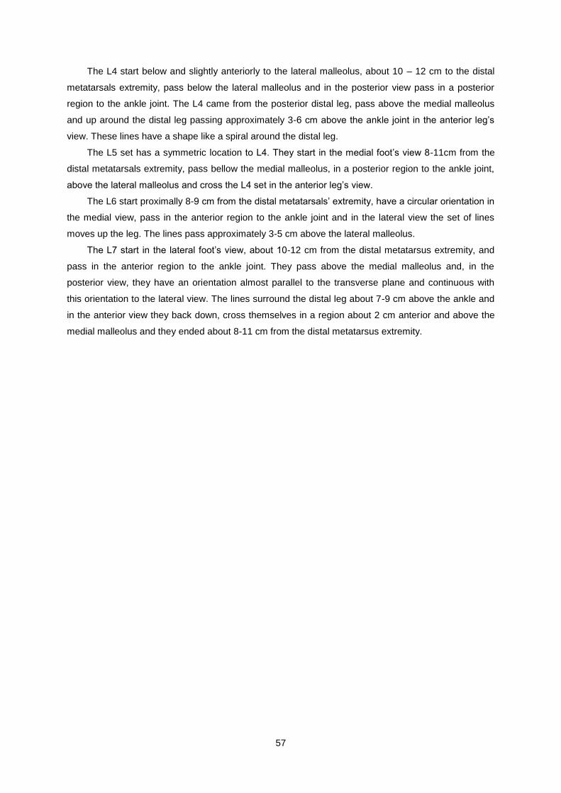
57
The L4 start below and slightly anteriorly to the lateral malleolus, about 10 – 12 cm to the distal
metatarsals extremity, pass below the lateral malleolus and in the posterior view pass in a posterior
region to the ankle joint. The L4 came from the posterior distal leg, pass above the medial malleolus
and up around the distal leg passing approximately 3-6 cm above the ankle joint in the anterior leg’s
view. These lines have a shape like a spiral around the distal leg.
The L5 set has a symmetric location to L4. They start in the medial foot’s view 8-11cm from the
distal metatarsals extremity, pass bellow the medial malleolus, in a posterior region to the ankle joint,
above the lateral malleolus and cross the L4 set in the anterior leg’s view.
The L6 start proximally 8-9 cm from the distal metatarsals’ extremity, have a circular orientation in
the medial view, pass in the anterior region to the ankle joint and in the lateral view the set of lines
moves up the leg. The lines pass approximately 3-5 cm above the lateral malleolus.
The L7 start in the lateral foot’s view, about 10-12 cm from the distal metatarsus extremity, and
pass in the anterior region to the ankle joint. They pass above the medial malleolus and, in the
posterior view, they have an orientation almost parallel to the transverse plane and continuous with
this orientation to the lateral view. The lines surround the distal leg about 7-9 cm above the ankle and
in the anterior view they back down, cross themselves in a region about 2 cm anterior and above the
medial malleolus and they ended about 8-11 cm from the distal metatarsus extremity.
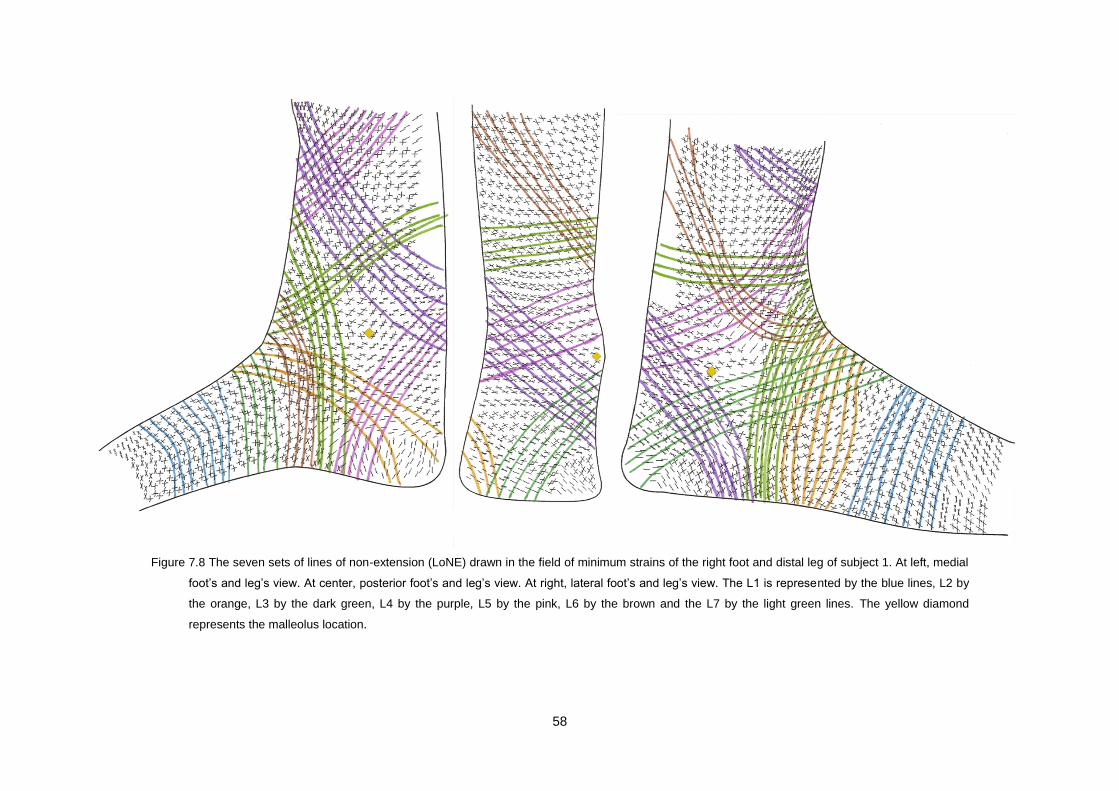
58
Figure 7.8 The seven sets of lines of non-extension (LoNE) drawn in the field of minimum strains of the right foot and distal leg of subject 1. At left, medial
foot’s and leg’s view. At center, posterior foot’s and leg’s view. At right, lateral foot’s and leg’s view. The L1 is represented by the blue lines, L2 by
the orange, L3 by the dark green, L4 by the purple, L5 by the pink, L6 by the brown and the L7 by the light green lines. The yellow diamond
represents the malleolus location.

59
Comparing the information from the principal strain field analyses and the locations of the LoNE is
possible to note that different sets of lines pass through the two regions of maximum deformations
(anterior region to the ankle joint and posterior region to Achilles’ tendon).
The sets L2, L3, L6 and L7 pass through the anterior region to the ankle joint. This skin’s region
suffers large extensions during plantar flexion and compressions during dorsiflexion, so, for an
orthosis to act like a second skin, it needs to perform large deformations along the longitudinal
direction in this region. The set L1, do not pass through a region of large deformations, but these lines
are important to support the foot’s weight mainly during swing period.
The sets L4 and L5 pass through the posterior region to the Achilles’ tendon, one of the foot’s
regions that suffer the largest foot’s skin deformation during the gait cycle. During plantar flexion this
region suffers the largest foot’s skin compressions and, during dorsiflexion, the largest skin’s
extensions.
The orthosis deformations are performed by actuators attached to them in the region where the
skin suffers large deformations. As the LoNE correspond to the directions in the skin where there is no
deformation, it is possible to pass through these directions inextensible wires without restriction of the
foot’s motion.
These wires are the best places to attach the actuators that will perform the orthosis deformations
(extensions and compressions). Moreover, not only the actuators can be placed in these wires but
also other important components, such as: movement sensors, to control the orthosis performance
during the different periods of the gait cycle, and electric wires to supply the actuators and sensors.
Finally, the lines’ extremities can be attached to the orthosis sole, which should be flexible and
adaptable to the foot’s motion.
7.4 Comparison of results with previous works
The first study of the lines of non-extension was performed by Iberall. During his research the LoNE
were found and mapped in the human skin, in particular, in the lower limb, but his study did not include
the ankle joint and the foot (Iberall 1964; Iberall 1970). More recently, at MIT, a spacesuit was
developed, the Bio-Suit, based on the concept of the LoNE. However, like the Iberall’s lines, for the
design of this spacesuit the LoNE in the ankle and foot were not calculated (Bethke 2005; Newman
2005).
60
Figure 7.9 At upper left, Iberall’s LoNE for the lower limb (Iberall 1970). At upper right,
representation of the anterior view of the Bio-Suit’s LoNE (Newman and Hoffman
2003). At bottom left, medial view of the right foot’s LoNE obtained in this study. At
bottom left, lateral view of the right foot’s LoNE obtained in this study.
The LoNE found by Iberall and the LoNE used in the Bio-Suit have, in the distal portion of the
lower limb, a configuration that forms a spiral around the leg and is clearly the existence of two types
of lines, one with a high inclination that spirals around the leg one time until it reaches the knee, and
another with a low inclination that spirals around the leg several times until it reaches the knee.
In this study, it were obtained three sets of LoNE (L4, L5, and L6) that have a spiral orientation in
the distal leg that continues upwards through this anatomical segment. All the directions of minimum
strain obtained above the ankle joint are directions of non-extension, with one of the directions having
a greater inclination through the leg than the other. These lines and directions of non-extension are
consistent and have continuity with the lines found by Iberall and the lines from the Bio-Suit (Figure
7.9).
61
Chapter 8
8. Conclusions and Future Developments
8.1 Conclusions
This thesis was developed with the main purpose of drawing the lines of non-extension (LoNE) in the
region of the ankle joint, to help in the development of an orthosis that will act like a second skin in the
drop-foot pathology correction. In order to draw the LoNE, it was necessary to map the skin’s strain
field during the ankle motion, dorsiflexion and plantar flexion, and to calculate the skin’s directions of
minimum strain from the skin’s deformation during these movements.
The skin’s deformation data, during plantar flexion and dorsiflexion, were acquired using a system
of four infrared cameras that calculated the trajectories of reflective markers placed on the skin. These
markers were placed in order to form an organized grid that covered all foot and distal leg, with the
exception of the sole. A computational program was developed to analyze the data from the skin’s
deformation that receives the information from the markers position in the initial and final (deformed)
foot’s configuration and, using finite elements, calculates the skin deformation. The obtained results
from the direct analysis of the original mesh’s data gave low information and the visual interpretation
was difficult to do, so, the analyses were performed with a refined mesh, which allowed a better
result’s visualization and interpretation.
The strain analyses were performed using a finite elements’ software that perform the calculus of
the deformation tensor for each element of the refined mesh using non-linear analysis due to the high
rigid body motions. The calculus of the magnitudes and directions’ of the principal strains and the
directions of the minimum strains were based in the Mohr’s circle equations.
The main difficulties in this study were due to acquisition problems. The acquisition system only
had four infrared cameras and this low number of cameras did not allow an acquisition of analyzed
regions as a whole at the same time, so the acquisitions had to be divided into different views of the
analyzed area. Another restriction, due to the acquisition system, was the original mesh refinement.
The minimum distance between the skin’s markers supported by the acquisition system is 2cm. An
original mesh with a greater refinement would have allowed a more accurate analysis of the skin’s
deformation. Despite the restrictions imposed by the acquisition system, it was possible to
successfully collect the data from the complete foot and distal leg’s surface.
In the analyses of the skin strain field, the expected results were obtained. Greater values of the
skin’s deformation were obtained in the anterior and posterior regions to the ankle joint, both in plantar
flexion and dorsiflexion movement. The anterior region to the ankle joint suffers the largest extensions
during plantar flexion and the largest compressions during dorsiflexion. The posterior region to the
ankle joint, in opposition to the anterior region, suffers the largest extensions during dorsiflexion and
the largest compressions during plantar flexion. Comparing the two analyzed movements, the
62
magnitudes of the skin’s deformation in these regions are greater in plantar flexion than in dorsiflexion
and, in both cases, the principal’s directions of deformation have longitudinal directions. The lowest
strains were obtained in the calcaneus region at approximately 6cm above the ankle joint.
From the analyses of the principal strain field, an analyses of the minimum strains’ direction, in
modulus, was performed. In these analyses, when one element just suffers compression, or
extension, just one direction of minimum strain, corresponding to the direction of the minimum
principal’s strain, in modulus. When the element suffers extension, in one direction, and compression
in another direction, two directions of minimum strain (directions of non-extension) were obtained. In
both analyses, dorsiflexion and plantar flexion, a larger density of directions of non-extension was
obtained in the analyzed skin’s surface. The regions where just one direction of minimum strain was
obtained corresponds to regions where there were more difficulties during the acquisition or in regions
were one of the principal’s direction has a value near zero. In the directions where one, or both, of the
principal strains are approximately zero, more inconsistencies between the directions of minimum
strain were obtained. This fact is maybe due to the greater influence of the noise of the marker’s
trajectories in the directions’ calculus. The low original mesh’s refinement was highly noted in the
obtained directions in the anterior region to the ankle joint and in the malleolus’ region. These regions
have an irregular shape, obtaining some inconsistencies in the directions of minimum strain between
the elements from the original mesh.
Despite having achieved some inconsistencies in the directions of minimum strain in some
regions, it was possible to draw the LoNE in the studied skin’s surface. Seven sets of LoNE were
found with the same anatomical orientation. Different sets pass through the two regions of larger
deformations. In the metatarsals region was found the only set of lines that do not go through any of
the two regions of maximum deformations, with a circumferential orientation.
Three of the others six sets of LoNE start and end in the sole, and one of them passes through the
leg. Finally, the other three sets of LoNE start in the foot’s sole and have an ascendant spiral
orientation through the leg. Two of the sets of LoNE that just start in the foot pass through the
posterior region to the ankle joint and all the other sets, except the one that is located in the
metatarsals region, go through the anterior region to the ankle joint. Any of these LoNE sets pass
through the malleolus regions because this region should not be restricted and is a region of low skin’s
deformation. The orientations of the three LoNE sets that have a spiral orientation through the leg are
consistent with the lines found by Iberall (Iberall 1970) and the lines used in the Bio-Suit spacesuit
(Newman and Hoffman 2003).
The sets of LoNE that go through the two regions of larger skin’s deformations are very important,
although these regions suffer large deformation during the foot’s motion, there are directions where
the skin does not deform and, in these directions, it is possible to pass inextensible wires without
restriction of the foot’s free motion. In these wires we can fix the orthosis actuators that will perform
the orthosis’ deformation and other orthosis components, such as movement sensors and electric
cables, without restricting the foot’s motion.

63
8.2 Future Developments
The major difficulties found during the development of this study were the impossibility to perform the
data acquisition with a more refined marker grid and to perform these acquisitions from all analyzed
skin surface at the same time. It is important to perform this study with a more refined mesh in order to
confirm the directions of the LoNE, mainly in the malleolus region and in the anterior region to the
ankle joint. This confirmation is only possible using an acquisition system with a larger number of
infrared cameras, or a different acquisition system which allows the use of a more refined mesh and a
total 3D acquisition.
The lack of time did not allow the development of a prototype to test the comfort and the freedom
of movement using a grid of inextensible wires with the orientations of the obtained lines of non-
extension. This test should be done before proceeding with more developments in the conception of
an orthosis based on the LoNE in order to test the validity of the use of these lines in an orthosis
design.
The development of an automatic computational process to draw the LoNE from the directions of
non-extension would allow, in an easy and fast way, the design of a grid of LoNE adapted to each
patient, improving the patient’s interaction and performance when using the orthosis.
Finally, for an orthosis to act as a second skin, it has to feel and react to the patient’s movements
and needs during his walk. The use of intelligent materials is a new and a good alternative to the
conventional materials but it still requires some research in this area.

64
65
References
Abaqus, Analysis User's Manual. Vol. I: Introduction, Spatial Modeling, Execution & Output. Version 6.7. 2007: ABAQUS, Inc.
Abas, W., Uniaxial tension test of human skin in vivo. Journal of Biomedical Engineering, 1982. 4(1): p. 65-71.
Abas, W., Biaxial tension test of human skin in vivo. Bio-Medical Materials andEngineering, 1994. 4(7): p. 473-486.
Agache, P. G., C. Monneur, J. L. Leveque and J. De Rigal, Mechanical Properties and Young's Modulus of Human Skin in Vivo. Archives of Dermatological Research, 1980. 269: p. 221-232.
Andriacchi, T. P., J. A. Ogle and J. O. Galante, Walking speed as a basis for normal and abnormal gait measurements. Journal of Biomechanics, 1977. 10(4): p. 261-268.
Association, A. H., Heart Disease and Stroke Statistics - 2009 Update. 2009, American Heart Association: Dallas, Texas.
Association, C.-M.-T. An Overview of Charcot-Marie-Tooth Disorders. 2010 [cited 20 September]; Available from: http://www.charcot-marie-tooth.org/about_cmt/overview.php.
Beer, F. P., E. R. Johnston and J. T. Dewolf, Mechanics of Materials. 3rd
ed. 2001: McGraw-Hill.
Berkelman, P., P. Rossi, T. Lu and J. Ma. Passive Orthosis Linkage for Locomotor Rehabilitation. in IEEE International Conference on Rehabilitation Robotics. 2007. Noordwijk, the Netherlands.
Bethke, K., The Second Skin Approach: Skin Strain Field Analysis and Mechanical Counter Pressure Prototyping for Advanced Spacesuit Design, in Department of Aeronautics and Astronautics. 2005, Massachusetts Institute of Technology. p. 26-30.
Blaya, J. A. and H. Herr, Adaptive Control of a Variable-Impedance Ankle-Foot Orthosis to Assist Drop-Foot Gait. IEEE Transactions on Neural Systems and Rehabilitation Engineering, 2004. 12(1): p. 24-31.
Bohannon, R. W., Strength of lower limb related to gait velocity and cadence in stroke patients. Physiotherapy Canada, 1986. 38(4): p. 204-206.
Britannica, E., Encyclopaedia Britannica. 2007.
Chin, R., E. T. Hsiao-Wecksler, E. Loth, G. Kogler, S. D. Manwaring, S. N. Tyson, K. A. Shorter and J. N. Gilmer, A pneumatic power harvesting ankle-foot orthosis to prevent foot-drop. Journal of NeuroEngineering and Rehabilitation, 2009. 6(19).
Cobeljic, G., M. Bumbasirevic, A. Lesic and Z. Bajin, The management of spastic equinus in cerebral palsy. Orthopaedics and Trauma, 2009. 23(3): p. 201-209.
Cua, A. B., K. P. Wilhelm and H. I. Maibach, Elastic properties of human skin: relation to age, sex, and anatomical region. Archives of Dermatological Research, 1990. 282: p. 283-288.
Dictionary, M. Anterior (A) and posterior (B) views of cleavage lines of the skin. 2010 [cited 2010 2 October]; Available from: http://medical-dictionary.thefreedictionary.com/lines+of+credit.
Dollar, A. M. and H. Hugh Herr. Active Orthoses for the Lower-Limbs: Challenges and State of the Art. in IEEE 10th International Conference on Rehabilitation Robotics. 2007. Noordwijk, The Netherlands.
66
Don, R., M. Serrao, P. Vinci, A. Ranavolo, A. Cacchio, F. Ioppolo, M. Paoloni, R. Procaccianti, F. Frascarelli and F. De Santis, Foot drop and plantar flexion failure determine different gait strategies in Charcot-Marie-Tooth patients. Clinical Biomechanics, 2007. 22(8): p. 905-916.
Eidelson, S. G. and S. Spinasanta. Drop Foot (Foot Drop) and Steppage Gait (Footdrop Gait). 2010 [cited 2010 September 12]; Available from: http://www.spineuniverse.com/conditions/sciatica/drop-foot-foot-drop-steppage-gait-footdrop-gait.
Elsner, P., E. Berardesca, K. P. Wilhelm and H. I. Maibach, Bioengineering of the Skin: Skin Biomechanics. Dermatology: Clinical & Basic Science Series. 2002: CRC Press LLC.
Escoffier, C., J. Rigal, A. Rochefort, R. Vasselet, J. L. Lévêque and P. G. Agache, Age-Related Mechanical Properties of Human Skin: An In Vivo Study. Journal of Investigative Dermatology, 1989. 93: p. 353-357.
Fatone, S., S. A. Gard and B. S. Malas, Effect of Ankle-Foot Orthosis Alignment and Foot-Plate Length on the Gait of Adults With Poststroke Hemiplegia. Archives of Physical Medicine and Rehabilitation, 2009. 9(5): p. 810-818.
Ferris, D. P., K. E. Gordon, G. S. Sawicki and A. Peethambaran, An improved powered ankle–foot orthosis using proportional myoelectric control. Gait and Posture, 2006. 23: p. 425-428.
Fitness, P. Buy a Running Shoe based on your Feet Arch Type. 2009 [cited 2010 1 October]; Available from: http://www.pinoyfitness.com/2009/12/buy-a-running-shoe-based-on-your-feet-arch-type/.
Geboers, J. F., M. R. Drost, F. Spaans, H. Kuipers and H. A. Seelen, Immediate and Long-Term Effects of Ankle-Foot Orthosis on Muscle Activity During Walking: A Randomized Study of Patients With Unilateral Foot Drop. Archives of Physical Medicine and Rehabilitation, 2002. 83: p. 240-245.
Gordon, N. F., M. Gulanick, F. Costa, G. Fletcher, B. A. Franklin, E. J. Roth and T. Shephard, Physical Activity and Exercise Recommendations for Stroke Survivors. Circulation, 2004. 109(16): p. 2031-2041.
Gray, H., Anatomy of the Human Body. 20 ed. 1918.
Hall, S. J., Basic Biomechanics. 2nd
ed. 1991: Mosby-Year Book, Inc.
Hendriks, F. M., Mechanical behaviour of human epidermal and dermal layers in vivo. 2005, Technische Universiteit Eindhoven: Eindhoven.
Hendriks, F. M., D. Brokken, C. W. J. Oomens, D. L. Bader and F. P. T. Baaijens, The relative contributions of different skin layers to the mechanical behavior of human skin in vivo using suction experiments. Medical Engineering and Physics, 2006. 28: p. 259–266.
Holt, B., A. Tripathi and J. Morgan, Viscoelastic response of human skin to low magnitude physiologically relevant shear. Journal of Biomechanics, 2008. 41: p. 2689-2695.
Holzapfel, G. A., Nonlinear Solid Mechinics: A Continuum Approach for Engineering. 2000: John Wiley and Sons Ltd.
Iberall, A. S., The Use of Lines of Nonextension to Improve Mobility in Full-Pressure Suits. 1964, Rand Development Corporation report to Behavioral Sciences Laboratory, Wright-Patterson AFB: Ohio.
Iberall, A. S., The Experimental Design of a Mibile Pressure Suit. Journal of Basic Engineering, 1970: p. 251-264.
67
Kuwazuru, O., J. Saothong and N. Yoshikawa, Mechanical approach to aging and wrinkling of human facial skin based on the multistage buckling theory. Medical Engineering and Physics, 2008. 30: p. 516–522.
Kwiatkowska, M., S. E. Franklin, C. P. Hendriks and K. Kwiatkowski, Friction and deformation behaviour of human skin. Wear, 2009. 267: p. 1264-1273.
Lam, W. K., J. C. Y. Leong, Y. H. Li, Y. Hu and W. W. Lu, Biomechanical and electromyographic evaluation of ankle foot orthosis and dynamic ankle foot orthosis in spastic cerebral palsy. Gait and Posture, 2005. 22: p. 189-197.
Langer, K., On the anatomy and physiology of the skin: I. The cleavability of the cutis. British Journal of Plastic Surgery, 1978. 31(1): p. 3-8.
Liu, Z. and K. Yeung, The Preconditioning and Stress Relaxation of Skin Tissue. Journal of Biomedical and Pharmaceutical Engineering, 2008. 2(1): p. 22-28.
Lockard, M. A., Foot Orthoses. Physical Therapy, 1988. 68(12): p. 1866-1873.
Mahmud, J., C. A. Holt and S. L. Evans, An innovative application of a small-scale motion analysis technique to quantify human skin deformation in vivo. Journal of Biomechanics, 2010. 43: p. 1002-1006.
Newman, D. J., Astronaut Bio-Suit System for Exploration Class Missions. 2005, Massachusetts Institute of Technology. p. 1-2.
Newman, D. J. and J. Hoffman, An Astronaut ‘Bio-Suit’ System: Exploration-Class Missions. 2003.
Pailler-Mattei, C., S. Bec and H. Zahouani, In vivo measurements of the elastic mechanical properties of human skin by indentation tests. Medical Engineering and Physics, 2008. 30: p. 599–606.
Perry, J., Gait Analysis: Normal and Pathological Function. 1992: SLACK incorporated.
Pritchett, J. W. and M. A. Porembski. Foot Drop. 2010 [cited 2010 4 September]; Available from: http://emedicine.medscape.com/article/1234607-overview.
Qualisys, ProReflex MCU - Qualisys Motion Capture Unit. Product Information. 2006.
Radtka, S. A., S. R. Skinner and M. E. Johanson, A comparison of gait with solid and hinged ankle-foot orthoses in children with spastic diplegic cerebral palsy. Gait and Posture, 2005. 21: p. 303-310.
Ring, H., I. Treger, L. Gruendlinger and J. M. Hausdorff, Neuroprosthesis for Footdrop Compared with an Ankle-Foot Orthosis: Effects on Postural Control during Walking. Journal of Stroke and Cerebrovascular Diseases, 2009. 18(1): p. 41-47.
Romkes, J. and R. Brunner, Comparison of a dynamic and a hinged ankle–foot orthosis by gait analysis in patients with hemiplegic cerebral palsy. Gait and Posture, 2002. 15(1): p. 18-24.
Rougier, P., C. Burdet, I. Farenc and L. Berger, How postural behaviour in undisturbed upright stance can be used to assess the physical characteristics of various models of ankle orthoses. Clinical Biomechanics, 2004. 19: p. 497-505.
Sanders, J. E., B. S. Goldstein and D. F. Leotta, Skin response to mechanical stress : Adaptation rather than breakdown—A review of the literature. Journal of Rehabilitation Research and Development, 1995. 32(3): p. 214–226.
Silver, F. H., L. M. Siperko and G. P. Seehra, Mechanobiology of force transduction in dermal tissue. Skin Research and Technology, 2003. 9(1): p. 3-23.
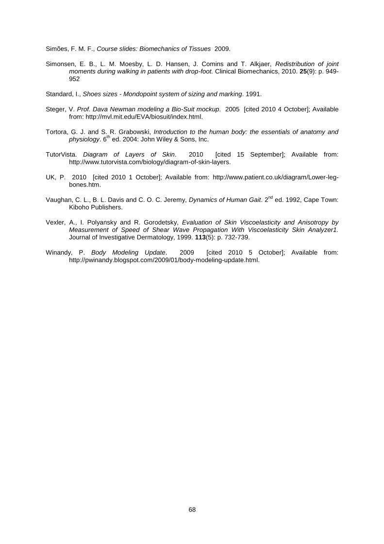
68
Simões, F. M. F., Course slides: Biomechanics of Tissues 2009.
Simonsen, E. B., L. M. Moesby, L. D. Hansen, J. Comins and T. Alkjaer, Redistribution of joint moments during walking in patients with drop-foot. Clinical Biomechanics, 2010. 25(9): p. 949-952
Standard, I., Shoes sizes - Mondopoint system of sizing and marking. 1991.
Steger, V. Prof. Dava Newman modeling a Bio-Suit mockup. 2005 [cited 2010 4 October]; Available from: http://mvl.mit.edu/EVA/biosuit/index.html.
Tortora, G. J. and S. R. Grabowski, Introduction to the human body: the essentials of anatomy and physiology. 6
th ed. 2004: John Wiley & Sons, Inc.
TutorVista. Diagram of Layers of Skin. 2010 [cited 15 September]; Available from: http://www.tutorvista.com/biology/diagram-of-skin-layers.
UK, P. 2010 [cited 2010 1 October]; Available from: http://www.patient.co.uk/diagram/Lower-leg-bones.htm.
Vaughan, C. L., B. L. Davis and C. O. C. Jeremy, Dynamics of Human Gait. 2nd
ed. 1992, Cape Town: Kiboho Publishers.
Vexler, A., I. Polyansky and R. Gorodetsky, Evaluation of Skin Viscoelasticity and Anisotropy by Measurement of Speed of Shear Wave Propagation With Viscoelasticity Skin Analyzer1. Journal of Investigative Dermatology, 1999. 113(5): p. 732-739.
Winandy, P. Body Modeling Update. 2009 [cited 2010 5 October]; Available from: http://pwinandy.blogspot.com/2009/01/body-modeling-update.html.

69
Appendix A
Figure A. 1 Lateral view of the directions of minimum strain from subject 1. A) 20TPF
movement. B) 40TPF movement. C) 60TPF movement. D) 80TPF movement. E)
100TPF movement.
Observing the anterior region to the ankle joint is possible to note that the angle between the two lines
of non-extension decreases with the increase of the movement’s amplitude until they become just one
line of minimum strain.
A B
C D
E
A
C

70
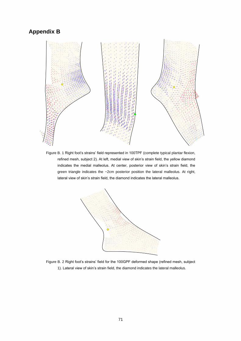
71
Appendix B
Figure B. 1 Right foot’s strains’ field represented in 100TPF (complete typical plantar flexion,
refined mesh, subject 2). At left, medial view of skin’s strain field, the yellow diamond
indicates the medial malleolus. At center, posterior view of skin’s strain field, the
green triangle indicates the ~2cm posterior position the lateral malleolus. At right,
lateral view of skin’s strain field, the diamond indicates the lateral malleolus.
Figure B. 2 Right foot’s strains’ field for the 100GPF deformed shape (refined mesh, subject
1). Lateral view of skin’s strain field, the diamond indicates the lateral malleolus.

72
Figure B. 3 Right foot’s strains’ field represented in 100TDF (complete typical dorsiflexion,
refined mesh, subject 2). At left, medial view of skin’s strain field, the yellow diamond
indicates the medial malleolus. At center, posterior view of skin’s strain field, the
green triangle indicates the ~2cm posterior position the lateral malleolus. At right,
lateral view of skin’s strain field, the diamond indicates the lateral malleolus.
Figure B. 4 Directions of minimum stretch during 100TPF (complete typical plantar flexion,
right foot, subject 2). Each line of the crosses correspond to one direction of non-
extension and each of the single lines correspond to the direction of minimum stretch
(extension or compression), when were not found directions of non-extension on the
element. At left, medial foot’s view, the yellow diamond corresponds to the medial
malleolus’ location. At center, posterior foot’s view, the green triangle indicates the
~2cm posterior position the lateral malleolus. At right, lateral foot’s view, the yellow
diamond corresponds to the lateral malleolus location.
73
Figure B. 5 Directions of minimum stretch during 100TDF (complete typical dorsiflexion, right
foot, subject 2). Each line of the crosses correspond to one direction of non-
extension and each of the single lines correspond to the direction of minimum stretch
(extension or compression), when were not found directions of non-extension on the
element. At left, medial foot’s view, the yellow diamond corresponds to the medial
malleolus’ location. At center, posterior foot’s view, the green triangle indicates the
~2cm posterior position the lateral malleolus. At right, lateral foot’s view, the yellow
diamond corresponds to the lateral malleolus location.