Sky Glow from Cities:

The Army Illumination Model v2

by Richard C. Shirkey

ARL-TR-5719 September 2011 Approved for public release; distribution is unlimited.

NOTICES

Disclaimers The findings in this report are not to be construed as an official Department of the Army position unless so designated by other authorized documents. Citation of manufacturer’s or trade names does not constitute an official endorsement or approval of the use thereof. Destroy this report when it is no longer needed. Do not return it to the originator.

Army Research Laboratory White Sands Missile Range, NM 88002-5501

ARL-TR-5719 September 2011

Sky Glow from Cities: The Army Illumination Model v2

Richard C. Shirkey

Computational and Information Sciences Directorate, ARL Approved for public release; distribution is unlimited.

ii

REPORT DOCUMENTATION PAGE Form Approved OMB No. 0704-0188

Public reporting burden for this collection of information is estimated to average 1 hour per response, including the time for reviewing instructions, searching existing data sources, gathering and maintaining the data needed, and completing and reviewing the collection information. Send comments regarding this burden estimate or any other aspect of this collection of information, including suggestions for reducing the burden, to Department of Defense, Washington Headquarters Services, Directorate for Information Operations and Reports (0704-0188), 1215 Jefferson Davis Highway, Suite 1204, Arlington, VA 22202-4302. Respondents should be aware that notwithstanding any other provision of law, no person shall be subject to any penalty for failing to comply with a collection of information if it does not display a currently valid OMB control number. PLEASE DO NOT RETURN YOUR FORM TO THE ABOVE ADDRESS.

1. REPORT DATE (DD-MM-YYYY)

September 2011 2. REPORT TYPE

Final 3. DATES COVERED (From - To)

FY09–FY11 4. TITLE AND SUBTITLE

Sky Glow from Cities: The Army Illumination Model v2 5a. CONTRACT NUMBER

5b. GRANT NUMBER

5c. PROGRAM ELEMENT NUMBER

6. AUTHOR(S)

Richard C. Shirkey 5d. PROJECT NUMBER

5e. TASK NUMBER

5f. WORK UNIT NUMBER

7. PERFORMING ORGANIZATION NAME(S) AND ADDRESS(ES)

U.S. Army Research Laboratory Computational and Information Sciences Directorate Battlefield Environment Division (ATTN: RDRL-CIE-M) White Sands Missile Range, NM 88002-5501

8. PERFORMING ORGANIZATION REPORT NUMBER

ARL-TR-5719

9. SPONSORING/MONITORING AGENCY NAME(S) AND ADDRESS(ES)

10. SPONSOR/MONITOR’S ACRONYM(S) 11. SPONSOR/MONITOR'S REPORT NUMBER(S)

12. DISTRIBUTION/AVAILABILITY STATEMENT

Approved for public release; distribution is unlimited.

13. SUPPLEMENTARY NOTES

14. ABSTRACT

The increasing number of people living on earth and the corresponding increase in outdoor lighting has resulted in light pollution—a brightening night sky that has obliterated the stars for much of the world’s population. However, for military purposes, in particular Night Vision Goggle (NVG) users, this light can allow for detection of targets that might ordinarily not be seen. The amount of light scattered from an urban location at night is a complicated function of light type, output and shielding, ground albedo, and the atmosphere that it must interact with. Clouds and various types of airborne particulates will also vary the amount of light received by NVGs. This report implements and extends the methods of Treanor and Garstang to estimate the light level received outside of urban locations. Clouds effects along with lunar and sky background illumination are included as are relevant data bases. 15. SUBJECT TERMS

urban illumination, clouds, target acquisition

16. SECURITY CLASSIFICATION OF: 17. LIMITATION

OF ABSTRACT

UU

18. NUMBER OF PAGES

48

19a. NAME OF RESPONSIBLE PERSON Richard C. Shirkey

a. REPORT

UNCLASSIFIED b. ABSTRACT

UNCLASSIFIED c. THIS PAGE

UNCLASSIFIED 19b. TELEPHONE NUMBER (Include area code) (575) 678-5470

Standard Form 298 (Rev. 8/98) Prescribed by ANSI Std. Z39.18

iii

Contents

List of Figures v

List of Tables vi

Acknowledgments vii

Executive Summary ix

1. Introduction 1

2. Background 2

2.1 Walker’s Law ..................................................................................................................2

2.2 Treanor’s Method ............................................................................................................2

2.3 Garstang’s Modifications ................................................................................................6

3. The Model 7

3.1 Basic Geometrical Equations ..........................................................................................7

3.2 Atmospheric Density .......................................................................................................8

3.3 Atmospheric Transmission ..............................................................................................9

3.4 Small Angle Scattering Approximation ........................................................................10

3.5 Brightness ......................................................................................................................10

3.6 Night Sky Background ..................................................................................................12

3.7 City Emission Function .................................................................................................13

3.8 Point vs. Extended Source .............................................................................................13

3.9 Limitations.....................................................................................................................14

4. Broadband Illumination Due to City Lights 15

4,1 Clear Skies .....................................................................................................................15

4.2 Cloudy Skies..................................................................................................................15

4.3 Lunar Illumination .........................................................................................................17

5. Spectral Composition of the Broadband Brightness 17

iv

5.1 City Light Types and Their Spectral Composition .......................................................17

5.2 Spectral Radiance ..........................................................................................................24

5.2.1 Contribution from City Lights ...........................................................................24

5.2.2 Contribution from Airglow ...............................................................................24

5.3 Conversion from Photopic to Radiometric Units ..........................................................25

6. Population and Location Database 25

7. Validation 25

7.1 Sky Brightness ...............................................................................................................25

7.2 Lunar Illumination .........................................................................................................26

7.3 Spectral Radiance ..........................................................................................................27

8. Future Work 28

9. References 29

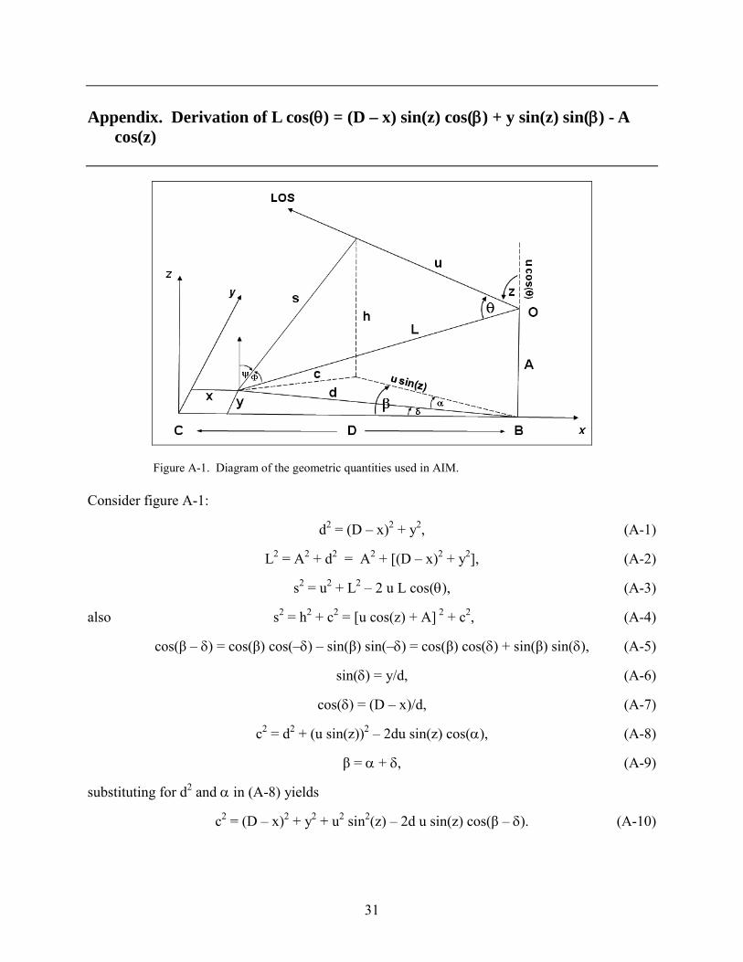
Appendix. Derivation of L cos(θ) = (D – x) sin(z) cos(β) + y sin(z) sin(β) - A cos(z) 31

List of Symbols, Abbreviations, and Acronyms 33

Distribution 34

v

List of Figures

Figure 1. Showing the locus of all points (dashed line) whose vertices form angles of a given size that contribute to the forward scattering received at collection point Z. ......................3

Figure 2. Geometry for determination of disk area Sd. X is the distance from T to Z and x is the distance from T to Sd. The scattering angle, , is assumed small. ...................................5

Figure 3. Light scattering from a city. Garstang's flat earth notation has been followed (4). .......8

Figure 4. Molecular number density (dashed line) and aerosol number density (solid line) as a function of height above sea level. ..........................................................................................9

Figure 5. Diagram for determination of luminance as seen from the observer. This figure is the expanded LOS portion of figure 3. ....................................................................................11

Figure 6. Geometry used for cloud cases. The cloud base, hc is indicated by the dashed line. ψ, Zo, Zm are the respective zenith angles for the city, observer and moon. The distances are represented from observer to point (x,y) by d, the LOS by Uc, and city to cloud by Sc. ....16

Figure 7. Spectrum for mercury vapor lamp. ................................................................................18

Figure 8. Spectrum for low pressure sodium. ...............................................................................19

Figure 9. Spectrum for high pressure sodium. ..............................................................................19

Figure 10. Spectrum for metal halide ceramic lamp. ....................................................................20

Figure 11. Spectrum for LED streetlight. .....................................................................................20

Figure 12. Spectrum for fluorescent tube or CFL. ........................................................................21

Figure 13. Spectrum for incandescent lamp. ................................................................................21

Figure 14. Spectrum for liquid kerosene.......................................................................................22

Figure 15. Spectrum for pressurized propane. ..............................................................................22

Figure 16. Airglow spectrum. .......................................................................................................23

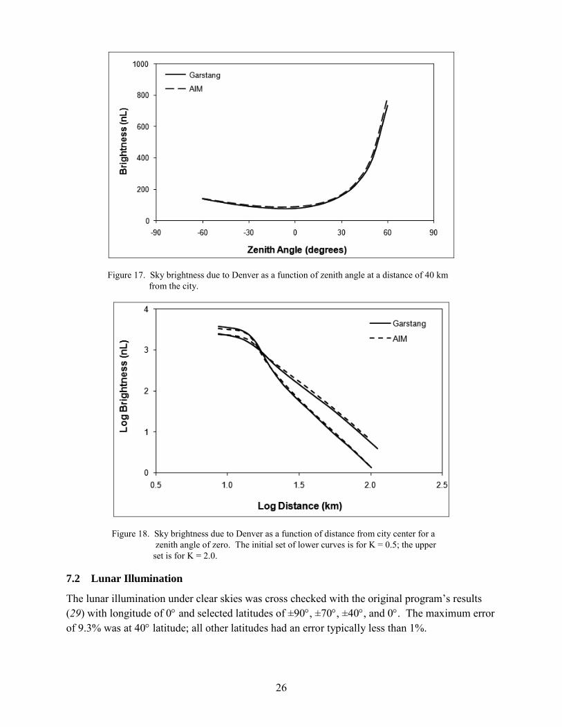
Figure 17. Sky brightness due to Denver as a function of zenith angle at a distance of 40 km from the city. ............................................................................................................................26

Figure 18. Sky brightness due to Denver as a function of distance from city center for a zenith angle of zero. The initial set of lower curves is for K = 0.5; the upper set is for K = 2.0. ........................................................................................................................................26

Figure 19. Results from AIM (dotted line) overlaid on the spectrum of Los Angeles as seen from Mt. Palomar in May 2005 under moonless conditions (solid line). Airglow is not included. (Courtesy Dr. Aube, University of Sherbrook, Canada). .........................................27

Figure 20. Results from AIM (dotted line) overlaid on the spectrum of Los Angeles as seen from Mt. Palomar in May 2005 under moonless conditions (solid line). Airglow has been included. (Courtesy Dr. Aubé, University of Sherbrook, Canada). .........................................28

Figure A-1. Diagram of the geometric quantities used in AIM. ...................................................31

vi

List of Tables

Table 1. Values for visibility and path length for a given value of K. .........................................15

Table 2. Cloud types available for high, middle, and low layers and their respective cloud base heights. .............................................................................................................................17

Table 3. Breakdown of street and flood lights in El Paso, TX and Las Cruces, NM 2007. ........23

Table 4. Los Angeles light types and estimated percent. ..............................................................27

vii

Acknowledgments

The author would like to thank Sean O’Brien, Dave Tofsted, Don Hoock, and Ed Measure for many hours of interesting and fruitful conversations leading to insights without which this program would never have seen the light of day.

viii

INTENTIONALLY LEFT BLANK.

ix

Executive Summary

With the U.S. Army’s increasingly fighting at night, it becomes necessary to know nighttime illumination levels before engagements occur, thereby providing mission planners the opportunity to select the most effective sensors under the expected illumination from urban settings. Helicopter pilots must be able to discern existing electrical wires; Soldiers need to know at what light level will they lose the ability to acquire targets; analysts need illumination levels to correctly analyze post-engagement situations for improved after action reports, and wargamers need such data for implementation in combat models.

The Army Illumination Model version 2 (AIM v2) is a full implementation of Garstang’s methodology for determining city brightness as a function of distance, look-angle, and city population and is a significant improvement over its predecessors: a preliminary Urban Illumination model and AIM v1. The model can calculate the brightness for either an extended or point source, depending on the observer’s distance from the city center. Brightness components include scattered radiation from the city, either from the clear atmosphere or reflected from a cloud deck, the ever present night sky background, and lunar illumination either passing through the clear atmosphere or a cloud deck. The cloud deck itself may contain typical cloud types for upper-, middle-, and lower-level clouds. The effects of illumination passing through this three-layer cloud deck are determined using Shapiro’s method for calculating the flux of lunar radiation through the atmosphere. In addition to the broadband brightness, spectral radiances are determined using light type spectral curves from a supplied file.

AIM v2 has been constructed for use with night vision devices, such as Night Vision Goggles (NVGs) and for use of, or incorporation into, the Infantry Warrior Simulation (IWARS) and the Target Acquisition Weapons Software (TAWS). Population plays a significant role in the amount of light emitted by any city and the light types used (mercury vapor, high pressure sodium, incandescent, etc.) greatly impact the spectral emission. While city populations are not difficult to obtain, they are still time-consuming to locate; the spectra of city light types is a challenge to obtain, particularly out to the wavelengths that night vision devices typically operate. Both of these data are included in ancillary data bases.

The program has been validated by comparison with Garstang’s results and with city spectra. This report contains detailed information on the physics and the approximations that were employed to construct the model. A separate report is available that details the numerical techniques and the usage of AIM v2.

x

INTENTIONALLY LEFT BLANK.

1

1. Introduction

Light pollution is defined as excessive and inappropriate artificial light comprised of four components, which are often combined and overlapping (1):

• Urban sky glow—the brightening of the night sky over inhabited areas.

• Light trespass—light falling where it is not intended, wanted, or needed.

• Glare—excessive brightness which causes visual discomfort. High levels of glare can decrease visibility.

• Clutter—bright, confusing, and excessive groupings of light sources, commonly found in over-lit urban areas. The proliferation of clutter contributes to urban sky glow, trespass, and glare.

Light trespass, glare and clutter components all contribute the urban sky glow, or simply sky glow, and are implicitly included in the techniques described in this report. Sky glow acts as an additional light source in the night sky faintly illuminating objects resulting in lowered visibility and changed contrast. To predict or model urban sky glow requires a complex and interrelated set of data: city size and output luminance, spectral content, number, and mean brightness of illumination sources, luminaries shielding, surface albedo and atmospheric aerosol content. Other influencing factors include cloud content and external illumination sources, such as moonlight, galactic light, auroral light, etc. Finally, but perhaps not surprisingly, population plays an important role in-so-far as the larger the population the larger are the lighting requirements for any given locale. A city’s economic state will also tend to affect the mean number of illumination sources present per inhabitant and the mean brightness per source. Other factors, such as nighttime blackout, may be dictated by tactical considerations.

For military operations, which are increasingly undertaken at night, locating targets and/or predicting their acquisition ranges requires knowing not only the sensor and target characteristics but also the weather conditions and the ambient illumination (sky glow). Sky glow strongly affects the ability of a sensor to “see” and determine acquisition ranges. In nighttime warfare, frequently the brightest sources of illumination are either from the moon or from urban areas. The received illumination from cities is further complicated by the presence of clouds, the reflection from which frequently is just as bright as that of a partial moon. For mission planning, training purposes, estimates of target acquisition ranges, and simulations such as IWARS, it is necessary to have an illumination model that will accurately simulate all of the above. City illumination models have been developed at varying levels of fidelity from research grade (2, 3), to those employing various approximations for multiple scattering, (4, 5, 6) to those that include clouds (7). The model described herein provides approximate, but reasonably accurate results, which include the effects of weather, clouds and varying populations.

2

2. Background

The problem of predicting the amount of light pollution or sky glow was first examined by astronomers concerned with choosing optimal locations for new observatories to avoid being hampered by the lack of dark skies. Summaries of recent work may be found in Garstang (8), Cinzano et al. (9) and Luginbuhl et al. (10, 11).

2.1 Walker’s Law

Walker (12) was the first to observationally link a city’s population with the amount of sky glow received at some distance outside of the city. Walker first consulted with municipal public works directors of cities in the vicinity of Mt. Palomar from which he was able to determine both the populations and total energy output of their street lights in lumens. From this data he found a linear relationship between luminosity L and the population of the city P or L ∝ P, known as the luminosity-population relation. Walker then took sky brightness measurements as a function of distance, DS, from Salinas, CA and was able to show that the city’s night sky brightness, or intensity, decreased proportional to the distance from Salinas raised to the −2.5 power,

I ∝ DS−2.5, (1)

known as the brightness-distance relationship. The exponent, –2.5, is reasonable considering that light propagation follows the inverse square law and atmospheric extinction will further attenuate the intensity. Using additional sky brightness measurements Walker (12) then found the distances, D, from these cities where the increase in artificial brightening at the zenith was ≤0.1 magnitude, and was able to relate this distance from the city to that city’s population as

P ∝ D2.5, (2)

known as the population-distance relationship. Garstang (8) reformulated equation 2 as

B = CPD−2.5 (3)

where B is the increase in sky glow level above the natural background and C is a coefficient that does not depend on P and D, but depends on factors, such as the light emission per head of the population and the reflectivity of the ground (8). Equation 3, known as Walker’s law, can be used to estimate sky glow and is the simplest model for light pollution.

2.2 Treanor’s Method

The first light pollution model was developed by Bertiau et al. (13) and Treanor (14) who proposed a small-angle approximation that accounts for single scattering effects. Treanor’s approximation accounts for the direct beam, scattering, and the attenuation of the direct and scattered light by absorption and scattering losses. The model assumptions and their rationale are:

3

• Homogeneous atmosphere:

• Aerosols are located predominantly in the lower atmosphere, and their distribution and amount is very irregular. However, radiative transfer codes that are capable of considering both the geometrical and physical effects and interactions are of research grade, complicated, and slow running. A homogeneous atmosphere ameliorates these problems considerably. If we exclude localized weather effects, such as thunderstorms, fog and other localized events, approximate results have been shown to provide reasonable results.

• Vertical heights are small in relation to the horizontal distance:

• If only point sources are considered then the vertical height of the scattering layers, which is usually a fraction of the troposphere, are small compared to the observer’s distance.*

• Scattering is limited to a cone of small angular extent whose axis of symmetry lies along the path of the direct beam and whose vertex, Q, is constrained to lie on arc TQY (see figure 1):

• Aerosol scattering at visible wavelengths is preferentially in the forward direction

• Flat earth:

• Curved-earth results differ by only 2% for distances less than 50 km.

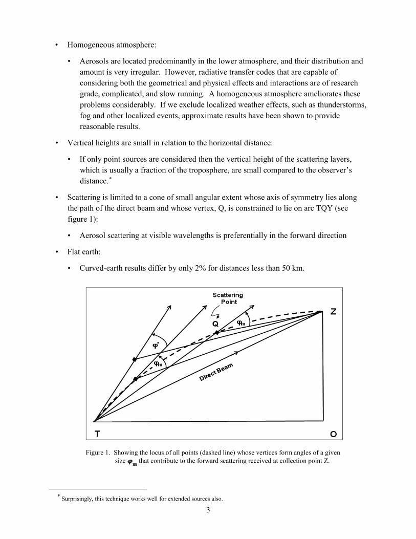
Figure 1. Showing the locus of all points (dashed line) whose vertices form angles of a given size that contribute to the forward scattering received at collection point Z.

* Surprisingly, this technique works well for extended sources also.

4

The basic scenario for Treanor’s model is an observer on the ground at some distance from a city considered to be a point source, and who is looking upward at the zenith. Consider figure 1 above, where T represents the town, O is the observer’s position (at ground level) and Z is the collection point (zenith) where the direct and scattered light is “received” and subsequently scattered downward to the observer. Since the city emission source, discussed in section 3.7, is a wide-spread intensity function emanating from point T, there are essentially an infinite number of outward “direct beams”, only one of which is relevant to the collection at Z (the direct beam) and is indicated in figure 1 by line TZ. If we constrain scattering to a forward direction within a cone of angle , where is small, then the locus of the scattering points will fall within the arc TQZ. The scattering points in the diagram are indicated by diamonds, one of which is labeled Q. One may easily see that scattering angles > cannot contribute scattered radiation at Z since the original premise is all scattering that occurs is within angles ≤ and must originate within the volume of rotation swept out by the arc TQZ about the direct beam line TZ. We note here, that while conceptually the forward scattering angle is the same as the angle through which the radiation is scattered into the observer’s line-of-sight (LOS), there is a distinct difference: , the forward scattering angle, is limited to some maximum angle , still small, whereas the angle through which the radiation is scattered into the observer’s LOS at point Z has no such restriction.

To determine the total scattered light received at Z, we confine the scattering to the forward direction, integrate over the direct beam path, and add up the contributions to the total forward scattering volume by a series of differentially thin disks of area Sd and thickness dx (see figure 2). Assuming a homogeneous atmosphere, and only accounting for forward scattering effects, the scattered contribution to the intensity from T impinging on and scattered from disk Sd at position x and received at Z is

(4)

where Io is the original intensity, N(h) is the particle density at height h, σ is the single particle scattering cross section, κ is the volume extinction coefficient, X is the distance from T to Z and x is the distance from T to Sd. The first term in parenthesis in equation 4 is the attenuated inverse square loss from T to Sd and the second term in parenthesis is the loss from Sd to Z.

5

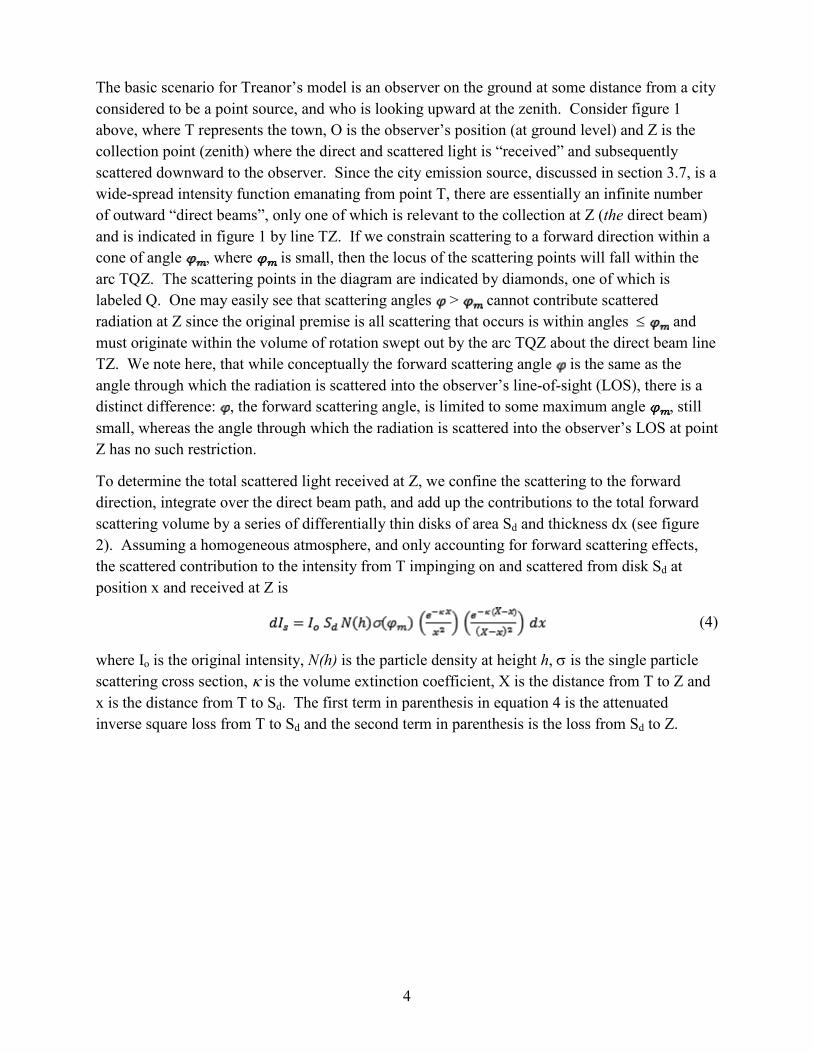
Figure 2. Geometry for determination of disk area Sd. X is the distance from T to Z and x is the distance from T to Sd. The scattering angle, , is assumed small.

To determine Sd we proceed as follows:

examination of figure 2 shows

, (5)

, (6)

solving for from equation 5 and substituting into equation 6 we find

, (7)

and, since is small, it follows that δ and ε are also small. Making use of the small angle approximation (SAA) we find

, (8)

and

. (9)

Combining (7), (8), and (9) and solving for r,

, (10)

and thus

. (11)

6

Since the atmosphere is homogeneous we can set σ(ϕ) = σ and rewrite (4) as

, (12)

where we have integrated over all scattering angles (see 2.3 below). Integrating equation 12 along the entire propagation path, the total integrated scattered intensity Is is

, (13)

and, upon adding in the direct beam we have for the final intensity at Z

, (14)

where ID is the direct beam intensity.

2.3 Garstang’s Modifications

Garstang (15, 16) modified Treanor’s constant scattering coefficient (σ) to allow an angular dependence of σ on the forward scattering angle ϕ, which allows Treanor’s factor π ϕ2 in equation 13 to be replaced with 2π ϕ dϕ. Since scattering at visible wavelengths is predominantly in the forward direction, the argument is made that σ( ) is small when is large and, therefore, we can replace σ( ) with σ, sans the dependence. Employing this approximation in conjunction with the SAA sin ϕ ≈ ϕ, we find that σi, the integrated scattering cross section for one particle of type i, to be

. (15)

Garstang further modified Treanor’s homogeneous atmosphere to one that decreases exponentially with height, is comprised of aerosols and molecules, and can be represented by

, (16)

where, for particles of type i, Ni (h) is the particle number density at height h, Ni(0) is the ground level density and ai is the particle-density reciprocal scale-height. Substituting equations 15 and 16 into equation 13 and, for a zenith angle z, we find

,

, (17)

after integration over x; h1 and h2 are heights and h = X cos z. To this we add the direct beam attenuation,

(18)

Equation 18 thus accounts for the inverse square law, the attenuation, and scattering (the second term in parenthesis). Garstang developed his model for both flat earth (4) and for a curved earth (16). The basic equations for Garstang’s flat-earth model were used in the construction of the

7

current model due both to its simplicity and Garstang’s determination (16) that curved-earth results differ by only 2% for distances less than 50 km from the city and for moderate zenith angles.

3. The Model

3.1 Basic Geometrical Equations

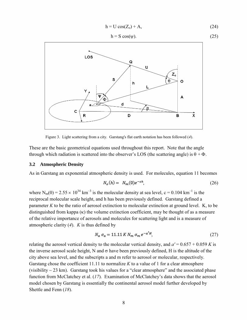
Figure 3 is the typical scenario used for flat earth calculations, where:

• O is the observer location at height A which projects downward to point B on the x-axis at a distance D from city center.

• C is the city center.

• a is an elemental area within the city’s radius R.

• d is the horizontal distance from observer to the elemental area, a, under consideration.

• L is the slant distance from the observer to the elemental area, a.

• U is the observer’s LOS.

• S is the upward light ray along which scattering is considered.

• Q is the scattering point between S and U.

• h is the vertical distance from Q to the x,y plane.

• Zo is the observer’s zenith angle (Zo = 0° when looking directly upward).

• θ is the angle between the observer’s LOS and L.

• ψ is the angle between the city’s zenith and Q.

• Φ is the angle between S and L.

• β is the azimuth angle of U as measured from the observer’s position (β is defined by the observer’s “look” direction: β = 0° when looking in the (user defined) forward direction; directly behind the observer β = 180°).

with these definitions, it can be shown that

d2 = (x – D)2 + y2, (19)

L2 = d2 + A2, (20)

L cos(θ) = (D – x) sin(Zo) cos(β) + y sin(Zo) sin(β) - A cos(Zo),† (21)

S2 = U2 + L2 - 2 U L cos(θ), (22)

L = S cos(Φ) + U cos(θ), (23)

† Equation 21 is derived in appendix A.

8

h = U cos(Zo) + A, (24)

h = S cos(ψ). (25)

Figure 3. Light scattering from a city. Garstang's flat earth notation has been followed (4).

These are the basic geometrical equations used throughout this report. Note that the angle through which radiation is scattered into the observer’s LOS (the scattering angle) is θ + Φ.

3.2 Atmospheric Density

As in Garstang an exponential atmospheric density is used. For molecules, equation 11 becomes

, (26)

where Nm(0) = 2.55 × 1034 km–3 is the molecular density at sea level, c = 0.104 km–1 is the reciprocal molecular scale height, and h has been previously defined. Garstang defined a parameter K to be the ratio of aerosol extinction to molecular extinction at ground level. K, to be distinguished from kappa (κ) the volume extinction coefficient, may be thought of as a measure of the relative importance of aerosols and molecules for scattering light and is a measure of atmospheric clarity (4). K is thus defined by

, (27)

relating the aerosol vertical density to the molecular vertical density, and a' = 0.657 + 0.059 K is the inverse aerosol scale height, N and σ have been previously defined, H is the altitude of the city above sea level, and the subscripts a and m refer to aerosol or molecular, respectively. Garstang chose the coefficient 11.11 to normalize K to a value of 1 for a clear atmosphere (visibility ~ 23 km). Garstang took his values for a “clear atmosphere” and the associated phase function from McClatchey et al. (17). Examination of McClatchey’s data shows that the aerosol model chosen by Garstang is essentially the continental aerosol model further developed by Shettle and Fenn (18).

9

The assumptions inherent in equation 27 should be borne in mind, vis-à-vis the following points:

• The molecular atmosphere is in hydrostatic equilibrium.

• The aerosol number density is an exponential function.

• The atmosphere is horizontally homogeneous.

• The atmospheric clarity parameter K relates the relative importance of aerosols to molecules.

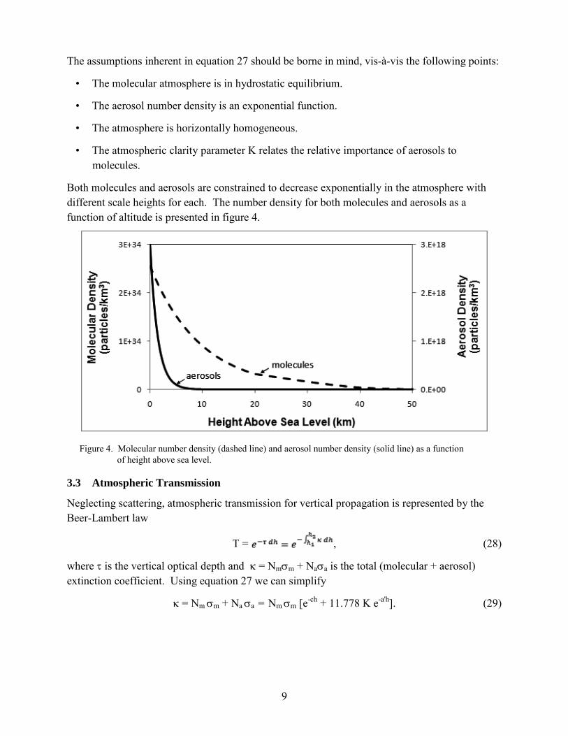
Both molecules and aerosols are constrained to decrease exponentially in the atmosphere with different scale heights for each. The number density for both molecules and aerosols as a function of altitude is presented in figure 4.

Figure 4. Molecular number density (dashed line) and aerosol number density (solid line) as a function of height above sea level.

3.3 Atmospheric Transmission

Neglecting scattering, atmospheric transmission for vertical propagation is represented by the Beer-Lambert law

T = , (28)

where τ is the vertical optical depth and κ = Nmσm + Naσa is the total (molecular + aerosol) extinction coefficient. Using equation 27 we can simplify

κ = Nm σm + Na σa = Nm σm [e-ch + 11.778 K e-a'h]. (29)

10

Using equation 28 and setting h1 to zero and h2 to an arbitrary height h, and making appropriate substitutions for κ we have

=

= . (30) This is the basic equation used for determination of transmission along the upward beam path S and the downward LOS path U. For the upward path and for the downward path h = U cos(z). The amount of scattering at point Q is determined by the Rayleigh (molecular) phase function plus the appropriate aerosol phase function. It should be noted that in Garstang’s 1986 paper (4) the stated curve fit to McClatchey’s phase function is incorrect; however, results from that paper indicate that a correct fit was used in the calculations.

3.4 Small Angle Scattering Approximation

Determination of multiple scattering from aerosols and/or molecules is frequently a time-consuming process requiring research grade codes thus giving rise to numerous simplifications and approximations. Garstang uses the approximation in equation 17 to represent what he calls “double scattering” along the upward path only. However, Garstang’s “double scattering” terminology is confusing and a misnomer. Garstang’s “double scattering” is another method in the bin of approximations that fall under the heading of SAA to the equation of radiative transfer. Referring to figure 3, in Garstang’s method scattering along path S is approximated by considering only those effects that arise from restricting scattering to a small angle in the forward direction. This approximation is applied only along the upward path S; a final single scattering takes place at point Q, where the radiation is scattered into the observer’s LOS for which there are no angular restrictions. Thus, we have small angle scattering along path S with a subsequent single scatter at point Q; attenuation, or extinction of the direct beam and the singly-scattered light into the LOS follows Beer’s law.

Considering the scattering portion of equation 17 we find the contribution of the scattered light to be

, (31)

where γ is a factor introduced by Garstang to account for the sphericity of Rayleigh scattering in comparison to aerosol scattering and the subscripts a and m refer to aerosol and molecular, respectively. Using equation 27 we simplify and write

(32)

3.5 Brightness

Since much of this work was first developed in the astronomical community, the prevalent system of units is photometric. Radiometry is the measurement of optical radiation whereas photometry, which predates radiometry, is the measurement of light, defined as electromagnetic radiation that is detectable by the human eye. Photometry is similar to radiometry except that

11

everything is weighted by the spectral response of the eye. Typical photometric units include lumens, lux, candelas, and a host of others. One can find a number of different definitions for brightness, dependent upon the community that one is conversing with. In this report, the brightness is in units of nanolamberts (1 lambert = 1 lumen/cm2), analogous to the Watt in radiometry. One lumen is defined as the luminous flux of light produced by a light source that emits one candela of luminous intensity over a solid angle of one steradian. In turn, luminous intensity, also a photometric measure, is a measure of the wavelength-weighted power emitted by a light source in a particular direction per unit solid angle. Luminous flux is often used as an objective measure of the useful power emitted by a light source, in our case, the city consisting of all light sources and types contained within the city’s radius.

We now determine the luminous flux, , as seen by an observer at point O in figure 3. Let be the emission function, considered spherically symmetric, for the city in the upward direction. Then the upward flux from an elemental area dx dy on the city disk is

, (33)

where β is the azimuth angle.

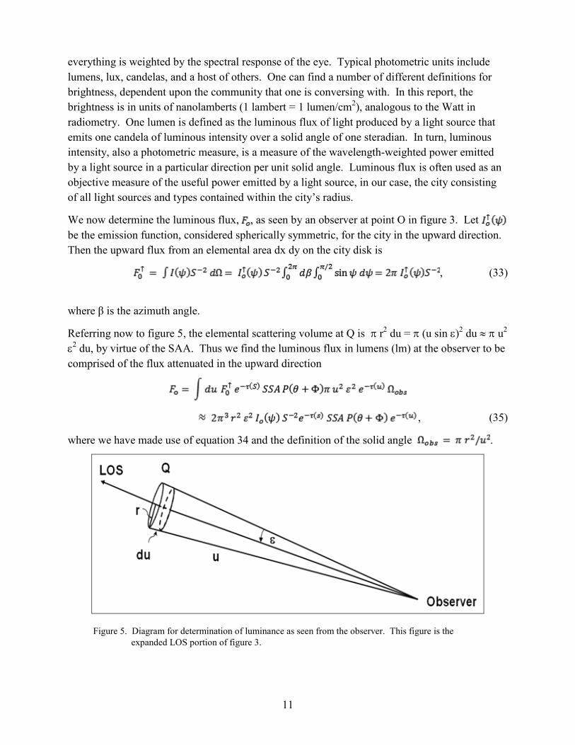
Referring now to figure 5, the elemental scattering volume at Q is π r2 du = π (u sin ε)2 du ≈ π u2 ε2 du, by virtue of the SAA. Thus we find the luminous flux in lumens (lm) at the observer to be comprised of the flux attenuated in the upward direction

, (35)

where we have made use of equation 34 and the definition of the solid angle .

Figure 5. Diagram for determination of luminance as seen from the observer. This figure is the expanded LOS portion of figure 3.

12

We know that the brightness, b, is the same at the source and at the detector. Hence the flux received at the observer from the surface at Q will be

(36)

The first factor in equation 36 represents the brightness in lm m–2 sr–1, the second factor is the area of the radiating surface, and the last factor is the solid angle as seen from the observer. Equating equation 35 and equation 36 and solving for the scattered brightness bs, we find

. (37)

To this we must add the direct beam, resulting in

. (38)

This is the equation for a point source; considering the city as a disk requires the additional double integration over dx dy; both options are available in the program.

A small but important point is the initial value of S at the start of the integration. If the initial value for S is too small, b becomes unrealistically large. To avoid this possibility a technique used in radiosity calculations is employed: S is initially set equal to 0.001 km for a point source and to 0.25 km for extended sources.

3.6 Night Sky Background

The glow of the (moonless) night sky comprises contributions from a number of sources including airglow, aurora, zodiacal light, starlight scattered by interstellar dust, extragalactic light, and light pollution from urban areas. Sections 3.1 through 3.5 dealt with the determination of light pollution from urban areas, but did not include any of the other aforementioned sources. The airglow, which is correlated to the solar sunspot cycle, is emitted by atoms and molecules in the upper atmosphere, which are excited by solar UV radiation during the day and is the brightest component of the light of the night sky. Aurora is a natural light display in the sky, particularly in the polar regions, caused by the collision of charged particles directed by the Earth's magnetic field and is negligible. Zodiacal light is sunlight scattered by interplanetary dust and contributes up to half the brightness of the night sky and starlight contributes substantially to the integrated brightness of the sky. Finally, the extragalactic contribution to the brightness of the night sky is very small. Benn and Ellison (19) have taken extensive measurements of these contributions and conclude that the night sky background brightness, Bnsb, can be well represented by

, (39)

where Bairglow, Bzodiacal, and Bstarlight are functions of the solar sunspot cycle, the ecliptic latitude, and the galactic latitude respectively. Bnsb is in S10 units (S10 is a bizarre astronomical unit of surface brightness corresponding to one 10th

magnitude star per square degree and will not be pursued further here). Benn and Ellison find that the sky brightness at La Palma, which they consider representative of other sites, is approximately 22 mag arcsec–2 or, using equation 19 from Garstang (4), ~17.6 nanolamberts (nL). From figure 3 in Garstang (4), “Sky brightness at

13

the zenith due to Denver as a function of the distance of the observer from Denver”, where the visibility ~48 km, shows that at a distance of ~70 km the brightness is ~18 nL. Since the sky background as determined by Benn and Ellison is comparable to the city sky glow from Denver at this large distance, it was deemed reasonable to set the value of Bnsb = 17.6 nL rather than carry out additional computations for only a small additional contribution to the total night sky brightness.

Since the primary contributor to the night sky brightness is the airglow produced by emissions from upper-air atoms and molecules it becomes necessary to consider its spectral contribution to the spectral radiance. In section 5 the methodology for determining the spectral radiance from the broadband radiance is presented; further discussion of the airglow spectra is discussed in that section.

3.7 City Emission Function

A last piece of information needed is an angular city “emission” function in the upward direction. Garstang (4) has used the following:

lm/sr, (40)

where script L and P are defined in equation 1, ψ is the city zenith angle as defined in figure 3, G is the surface albedo and F is the fraction of the light emitted by fixtures in an upward direction. Within the curly brackets the factor of 2 in the first term and the factor of 0.554 in the second term are normalization constants. Cinzano (20) has investigated variants of the city emission function and finds little difference in the resultant sky luminance. Garstang (4) found that a value of L ≅ 1000 lumens per capita fit Walker’s data (12) well. However, Luginbuhl (10, 11), who has acquired a massive amount of lighting data for the city of Flagstaff, found that the average value of L for Flagstaff was ~2500 lumens per capita, considerably different from Garstang’s. Luginbuhl hypothesizes that this discrepancy can be accounted for by considering the effects of secondary scattering from buildings and blocking from terrain and vegetation, factors which Garstang did not consider. Luginbuhl (11) proposed a modified form of Garstang’s emission function (equation 40)

, (41)

where Eb is a blocking factor at the zenith and is a “unblocking” factor added to account for the discrete nature of the obscuring objects (buildings, etc.). Thus allows for more light to be available at the high zenith angles encountered when viewing in a horizontal direction. Luginbuhl found that the best fits for Flagstaff were Eb ≅ 0.45 and = 0.0. However, there are numerous problems with this approach (intensity goes to zero at the horizon, objects producing near-ground blocking are purely absorptive, etc.) and it has not been implemented in the model.

3.8 Point vs. Extended Source

As we approach a city from some large distance the assumption of the source as a point becomes invalid. While the methodology enumerated above is applicable to both point and extended

14

sources the computational methods differ requiring that some consistent method be used to ascertain at what distance this change occurs. The following discussion addresses this concern.

Referring again to figure 3, consider the city as a extended-area Lambertian light source and a point source co-axial with and perpendicular to that source located a distance, D, away. The irradiance, Ee, at that point in a plane perpendicular to the axis, due to the extended-area source with a radius, R, can be shown to be (21):

Ee = πL'R 2 / (R 2 + D 2), (42)

where, L', is the radiance of the extended-area source. Now, for R << D, the irradiance of a co-axial point, Ep, will fall off with the distance, D, as

Ep = πL'R 2 / D 2. (43)

To gain insight into the distance where the approximation of an extend source as a point begins to break down, we proceed as follows. Let the acceptable error between Ee and Ep be ε. Then from equation 42 and equation 43 we easily find

ε = D2/R2. (44)

This then provides a criterion for differentiating between an extended source and a point source. Solving for D, the final determiner becomes

D ≥ R ε−½. (45)

Thus for given R and ε, the approximation for a point source is only valid for D such that equation 45 holds; in the model ε was taken as 0.20 (20%) implying that D must satisfy the condition of being greater than or equal to ≈ 2.25 R.

3.9 Limitations

It can be shown (4) that the horizontal visibility is

, (46)

where H is the height of the city above sea level. This equation allows us to determine the visibility for the various values of K that Garstang uses. The horizontal optical depth for path length d is

, (47)

and the limit of the applicability of single scattering techniques is usually considered to be τ ≤ 1.0. Using equations 46 and 47, table 1 presents visibilities and horizontal distances valid for τ ≤ 1.0.

15

Table 1. Values for visibility and path length for a given value of K.

K Vis (km) d (km) 0.5 48 12.4 2.0 14 3.5 3.0 9.2 2.4

Thus, for a K value of 2.0, the visibility is 14 km valid for path lengths less than or equal to 3.5 km (i.e., multiple scattering effects will influence the results for path lengths greater than 3.5 km when the visibility is 14 km).

4. Broadband Illumination Due to City Lights

4,1 Clear Skies

When no clouds are present Garstang’s model as presented in section 3 is used to calculate the scattering along the beam axis using the SAA. This radiation is then scattered into the LOS using the Rayleigh and aerosol single-scattering phase functions. Attenuation is considered along both the upward and downward (LOS) paths for a maximum distance of 40 km.

4.2 Cloudy Skies

Prediction of illumination under realistic atmospheric conditions that include partly cloudy and overcast conditions and fog/smoke is handled by a modified version of the ILUMA model (22). ILUMA uses traditional surface observations that report the type of cloud and percent cloud cover in the standard low, middle and upper, or high, atmospheric levels in conjunction with Shapiro’s model (23) which uses the doubling method to calculate the flux of solar radiation passing through the clouds and impinging on the surface. The input for the three-layer model consists of the cloud type and fraction for each of the three layers and the surface albedo. Within these three layers, Shapiro found that there was little difference between some of the cloud types and subsequently classified them into four cloud groups: cirrus (Ci)/cirrostratus (Cs), altostratus (As)/altocumulus (Ac), cumulus (Cu)/cumulonimbus (Cb), and stratus (St)/stratocumulus (Sc). The overall layer scheme is as follows:

• High―clear, thin and thick Ci/Cs

• Medium―clear, As/Ac

• Low―clear, clear (f/k), Cu/Cb or St/Sc

where (f/k) indicates fog or smoke reported.

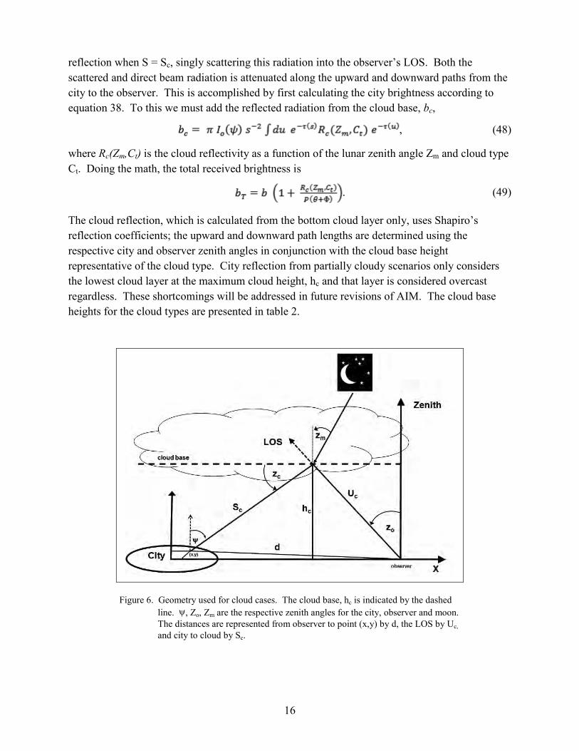
When clouds are present the total city brightness is calculated in two separate pieces using the Garstang model in conjunction with the Shapiro model. Referencing figure 6, scattering is considered along upward path Sc, where Sc is constrained by the cloud ceiling, or base, height. The total brightness is found by calculating the scattering along Sc coupled with the cloud

16

reflection when S = Sc, singly scattering this radiation into the observer’s LOS. Both the scattered and direct beam radiation is attenuated along the upward and downward paths from the city to the observer. This is accomplished by first calculating the city brightness according to equation 38. To this we must add the reflected radiation from the cloud base, bc,

, (48)

where Rc(Zm,Ct) is the cloud reflectivity as a function of the lunar zenith angle Zm and cloud type Ct. Doing the math, the total received brightness is

. (49)

The cloud reflection, which is calculated from the bottom cloud layer only, uses Shapiro’s reflection coefficients; the upward and downward path lengths are determined using the respective city and observer zenith angles in conjunction with the cloud base height representative of the cloud type. City reflection from partially cloudy scenarios only considers the lowest cloud layer at the maximum cloud height, hc and that layer is considered overcast regardless. These shortcomings will be addressed in future revisions of AIM. The cloud base heights for the cloud types are presented in table 2.

Figure 6. Geometry used for cloud cases. The cloud base, hc is indicated by the dashed line. ψ, Zo, Zm are the respective zenith angles for the city, observer and moon. The distances are represented from observer to point (x,y) by d, the LOS by Uc, and city to cloud by Sc.

17

Table 2. Cloud types available for high, middle, and low layers and their respective cloud base heights.

Layer Cloud Type Cloud Base (km)

Hig

h

Clear 40.0

Thin Ci/Cs 9.3

Thick Ci/Cs 9.3

Mid

dle Clear 40.0

As/Ac 4.0 Lo

w

Clear 40.

Clear w fog/smoke

40

Sc/St 1.1

Cu/Cb 1.2

4.3 Lunar Illumination

Lunar illumination is determined as a function of location, time, and phase angle of the moon. For a selected date and city location, the lunar illumination, either through the atmosphere or through clouds, is calculated using Shapiro’s algorithm as detailed in Shapiro (23).

5. Spectral Composition of the Broadband Brightness

Once the broadband brightness is determined it is broken down spectrally by the following procedure (24). The spectral composition of urban light is determined by identifying the types of lights used in typical cities and estimating the percentage that each light source contributes to the overall city light source. The spectral radiance values over the sensor’s waveband are calculated based on the city brightness amount due to each individual light source.

5.1 City Light Types and Their Spectral Composition

The types of lights that comprise urban settings and their spectral content must be known for the model to function (i.e., a lighting database of some nature is required). In any given city many light types are employed on city streets, highways, office buildings, shopping centers, stadiums, houses, parking lots, etc. The resulting mix of light is highly heterogeneous due to the variety of light source spectra, the effects of atmospheric scattering and absorption, and reflection from the ground. The mix contains both a broad continuum of radiation along with many superimposed

18

emission lines at specific wavelengths. Beyond 0.5 µm, metal halide and high pressure sodium lamps are the primary contributors to the city light continuum. While it was desired to include light types external to U.S. manufacture, an extensive examination of the available literature was unable to distinguish any significant differences in light types currently in use between American or non-American manufacturers. However, cultural and/or economic differences may dictate different light type usage.

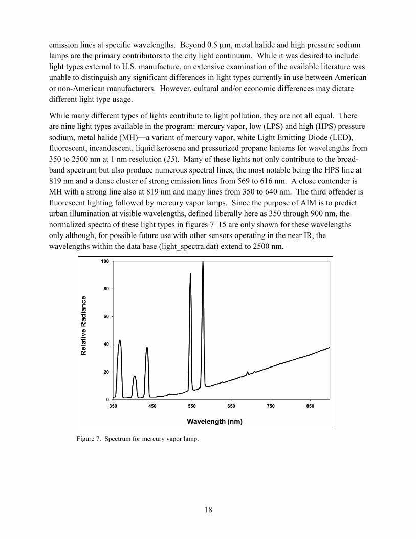
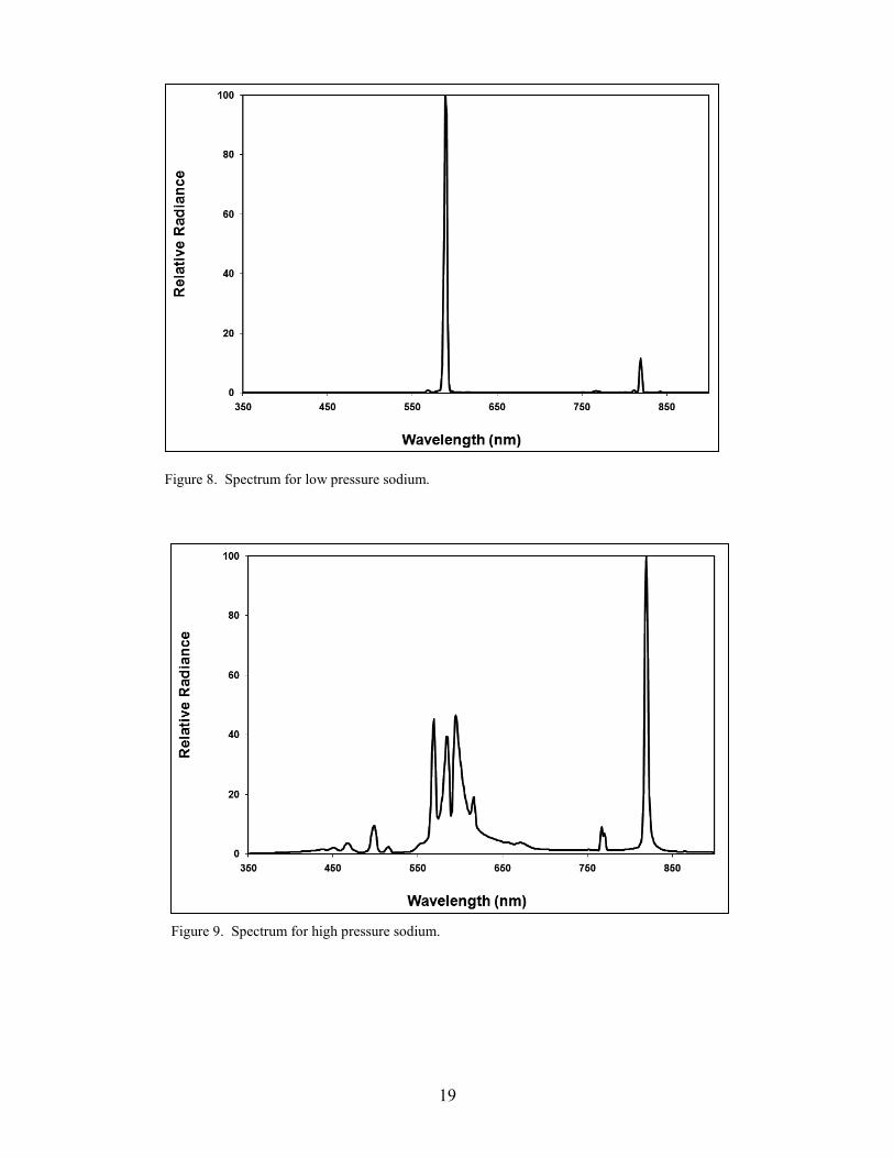
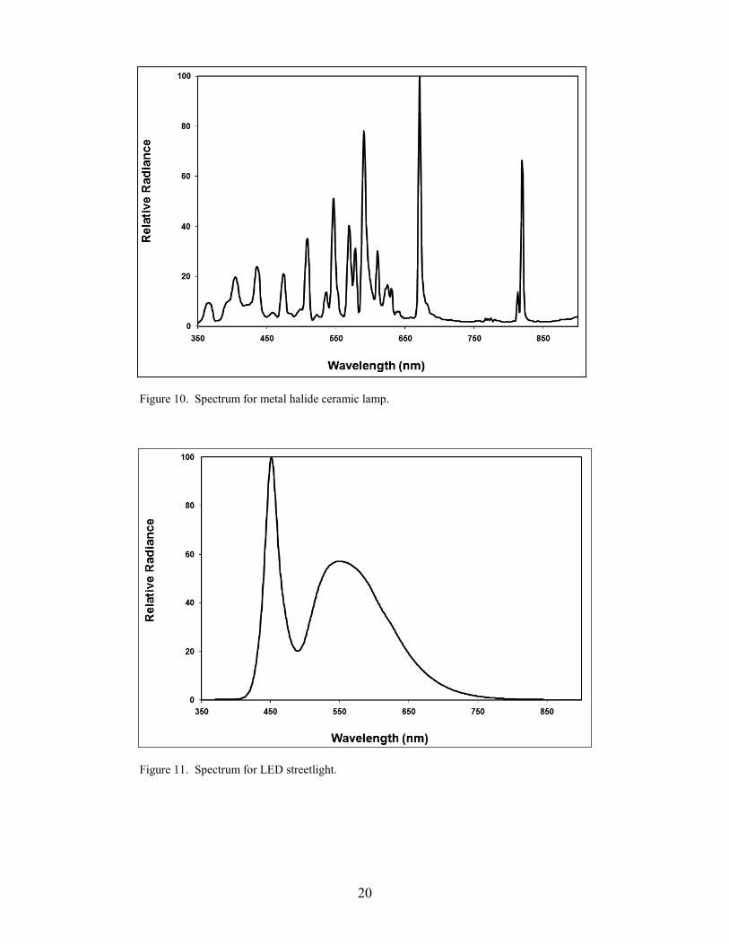
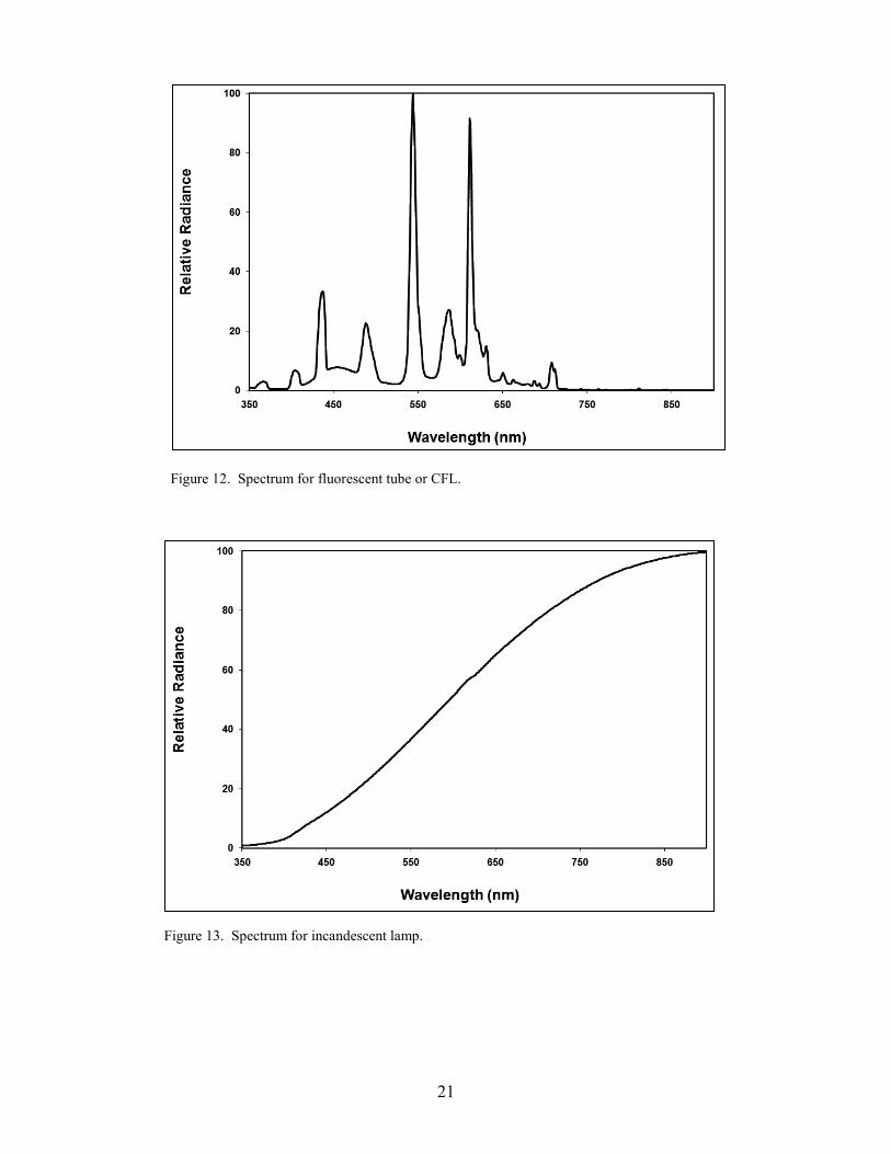
While many different types of lights contribute to light pollution, they are not all equal. There are nine light types available in the program: mercury vapor, low (LPS) and high (HPS) pressure sodium, metal halide (MH)―a variant of mercury vapor, white Light Emitting Diode (LED), fluorescent, incandescent, liquid kerosene and pressurized propane lanterns for wavelengths from 350 to 2500 nm at 1 nm resolution (25). Many of these lights not only contribute to the broad-band spectrum but also produce numerous spectral lines, the most notable being the HPS line at 819 nm and a dense cluster of strong emission lines from 569 to 616 nm. A close contender is MH with a strong line also at 819 nm and many lines from 350 to 640 nm. The third offender is fluorescent lighting followed by mercury vapor lamps. Since the purpose of AIM is to predict urban illumination at visible wavelengths, defined liberally here as 350 through 900 nm, the normalized spectra of these light types in figures 7–15 are only shown for these wavelengths only although, for possible future use with other sensors operating in the near IR, the wavelengths within the data base (light_spectra.dat) extend to 2500 nm.

Figure 7. Spectrum for mercury vapor lamp.

19

Figure 8. Spectrum for low pressure sodium.

Figure 9. Spectrum for high pressure sodium.

20

Figure 10. Spectrum for metal halide ceramic lamp.

Figure 11. Spectrum for LED streetlight.

21

Figure 12. Spectrum for fluorescent tube or CFL.

Figure 13. Spectrum for incandescent lamp.

22

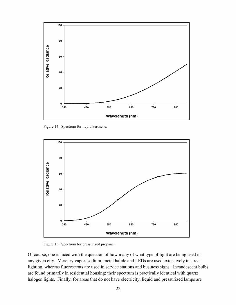
Figure 14. Spectrum for liquid kerosene.

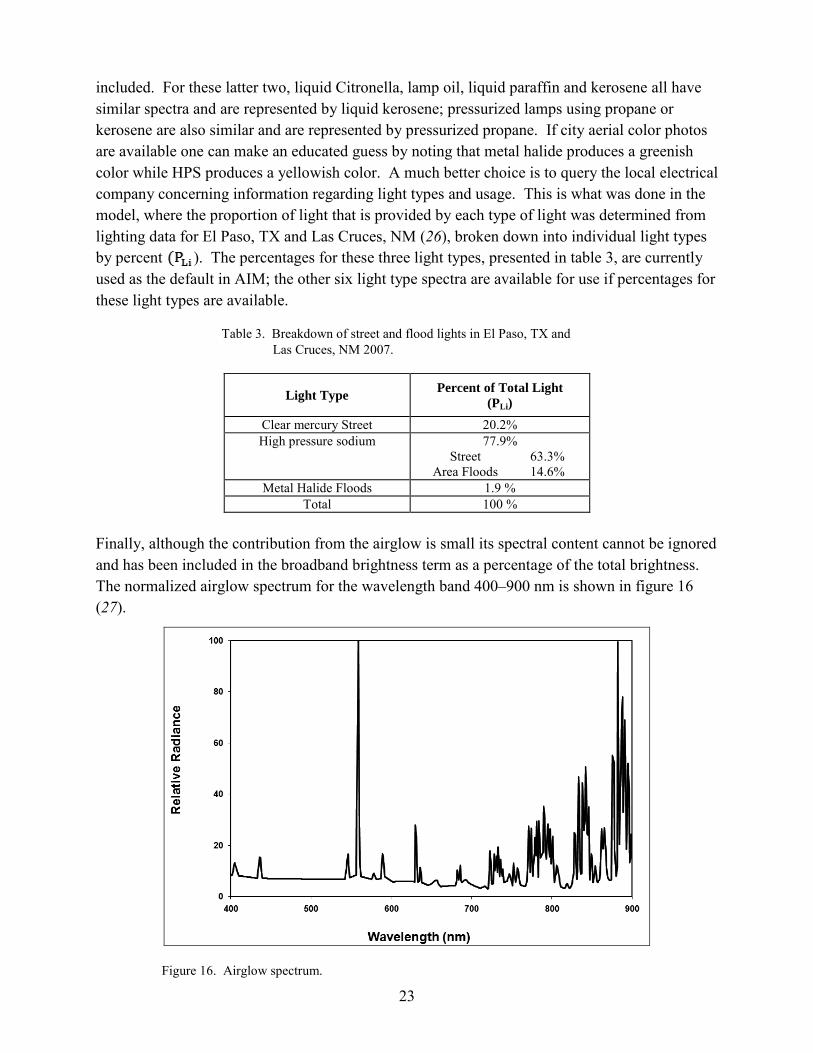
Figure 15. Spectrum for pressurized propane.

Of course, one is faced with the question of how many of what type of light are being used in any given city. Mercury vapor, sodium, metal halide and LEDs are used extensively in street lighting, whereas fluorescents are used in service stations and business signs. Incandescent bulbs are found primarily in residential housing; their spectrum is practically identical with quartz halogen lights. Finally, for areas that do not have electricity, liquid and pressurized lamps are

23

included. For these latter two, liquid Citronella, lamp oil, liquid paraffin and kerosene all have similar spectra and are represented by liquid kerosene; pressurized lamps using propane or kerosene are also similar and are represented by pressurized propane. If city aerial color photos are available one can make an educated guess by noting that metal halide produces a greenish color while HPS produces a yellowish color. A much better choice is to query the local electrical company concerning information regarding light types and usage. This is what was done in the model, where the proportion of light that is provided by each type of light was determined from lighting data for El Paso, TX and Las Cruces, NM (26), broken down into individual light types by percent ). The percentages for these three light types, presented in table 3, are currently used as the default in AIM; the other six light type spectra are available for use if percentages for these light types are available.

Table 3. Breakdown of street and flood lights in El Paso, TX and Las Cruces, NM 2007.

Light Type Percent of Total Light (PLi)

Clear mercury Street 20.2% High pressure sodium 77.9%

Street 63.3% Area Floods 14.6%

Metal Halide Floods 1.9 % Total 100 %

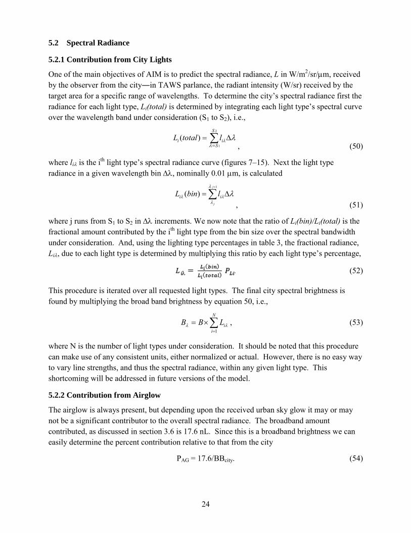
Finally, although the contribution from the airglow is small its spectral content cannot be ignored and has been included in the broadband brightness term as a percentage of the total brightness. The normalized airglow spectrum for the wavelength band 400–900 nm is shown in figure 16 (27).

Figure 16. Airglow spectrum.

24

5.2 Spectral Radiance

5.2.1 Contribution from City Lights

One of the main objectives of AIM is to predict the spectral radiance, L in W/m2/sr/µm, received by the observer from the city―in TAWS parlance, the radiant intensity (W/sr) received by the target area for a specific range of wavelengths. To determine the city’s spectral radiance first the radiance for each light type, Li(total) is determined by integrating each light type’s spectral curve over the wavelength band under consideration (S1 to S2), i.e.,

∑=

∆=2

1

)(S

Sii ltotalL

λλλ

, (50)

where liλ is the ith light type’s spectral radiance curve (figures 7–15). Next the light type radiance in a given wavelength bin ∆λ, nominally 0.01 µm, is calculated

∑

+

∆=1

)(j

j

ii lbinLλ

λλλ λ

, (51)

where j runs from S1 to S2 in ∆λ increments. We now note that the ratio of Li(bin)/Li(total) is the fractional amount contributed by the ith light type from the bin size over the spectral bandwidth under consideration. And, using the lighting type percentages in table 3, the fractional radiance, Liλ, due to each light type is determined by multiplying this ratio by each light type’s percentage,

. (52)

This procedure is iterated over all requested light types. The final city spectral brightness is found by multiplying the broad band brightness by equation 50, i.e.,

∑

=

×=N

iiLBB

1λλ , (53)

where N is the number of light types under consideration. It should be noted that this procedure can make use of any consistent units, either normalized or actual. However, there is no easy way to vary line strengths, and thus the spectral radiance, within any given light type. This shortcoming will be addressed in future versions of the model.

5.2.2 Contribution from Airglow

The airglow is always present, but depending upon the received urban sky glow it may or may not be a significant contributor to the overall spectral radiance. The broadband amount contributed, as discussed in section 3.6 is 17.6 nL. Since this is a broadband brightness we can easily determine the percent contribution relative to that from the city

PAG = 17.6/BBcity. (54)

25

This amount is added to the city spectral radiance as determined by equation 53 resulting in a received spectral radiance of

)(

1AG

TotalAG

AGN

ii P

LLLBB ×+×= ∑

=

λλλ

(55)

5.3 Conversion from Photopic to Radiometric Units

The final step in calculating the radiance contribution due to urban illumination is to convert from photometric units (nL) to radiometric units (W/m2/sr/µm). Equation 56 was used for the final conversion

B (W/m2/sr/µm) = B (nL/µm) × 1.464×10–8. (56)

6. Population and Location Database

Since population is an integral input for the model, a limited database (cities_info.dat) is provided with the program to supply not only the population of various worldwide cities, but also their latitude and longitude in decimal degrees. Given that the population is the main driver of city illumination, where possible the metropolitan area population, rather than the city population itself, was used. The available cities, as well as their latitude and longitude, may be found in appendix B of Shirkey (28). If the user desired city is not in the database, the user is asked to enter the population and latitude and longitude of that city, which may then be optionally entered into the database by the user. Many additional latitudes, longitudes and populations for worldwide cities may be found at http://www.wikipedia.org/.

7. Validation

7.1 Sky Brightness

Validation was done via comparison with results from Garstang (4). His figures 2 and 3 were digitized and compared with model values computed for the same location and geometries. Figure 17 shows brightness as a function of zenith angle for the city of Denver; the distance was fixed at 40 km. Garstang’s figure 3 was also compared with AIM v2 with results presented in figure 18.

26

Figure 17. Sky brightness due to Denver as a function of zenith angle at a distance of 40 km from the city.

Figure 18. Sky brightness due to Denver as a function of distance from city center for a zenith angle of zero. The initial set of lower curves is for K = 0.5; the upper set is for K = 2.0.

7.2 Lunar Illumination

The lunar illumination under clear skies was cross checked with the original program’s results (29) with longitude of 0° and selected latitudes of ±90°, ±70°, ±40°, and 0°. The maximum error of 9.3% was at 40° latitude; all other latitudes had an error typically less than 1%.

27

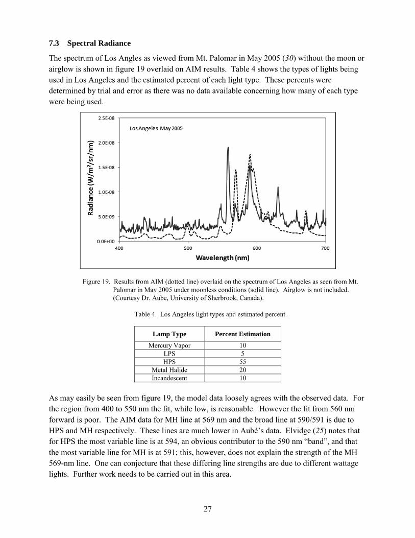
7.3 Spectral Radiance

The spectrum of Los Angles as viewed from Mt. Palomar in May 2005 (30) without the moon or airglow is shown in figure 19 overlaid on AIM results. Table 4 shows the types of lights being used in Los Angeles and the estimated percent of each light type. These percents were determined by trial and error as there was no data available concerning how many of each type were being used.

Figure 19. Results from AIM (dotted line) overlaid on the spectrum of Los Angeles as seen from Mt. Palomar in May 2005 under moonless conditions (solid line). Airglow is not included. (Courtesy Dr. Aube, University of Sherbrook, Canada).

Table 4. Los Angeles light types and estimated percent.

Lamp Type Percent Estimation

Mercury Vapor 10 LPS 5 HPS 55

Metal Halide 20 Incandescent 10

As may easily be seen from figure 19, the model data loosely agrees with the observed data. For the region from 400 to 550 nm the fit, while low, is reasonable. However the fit from 560 nm forward is poor. The AIM data for MH line at 569 nm and the broad line at 590/591 is due to HPS and MH respectively. These lines are much lower in Aubé’s data. Elvidge (25) notes that for HPS the most variable line is at 594, an obvious contributor to the 590 nm “band”, and that the most variable line for MH is at 591; this, however, does not explain the strength of the MH 569-nm line. One can conjecture that these differing line strengths are due to different wattage lights. Further work needs to be carried out in this area.

28

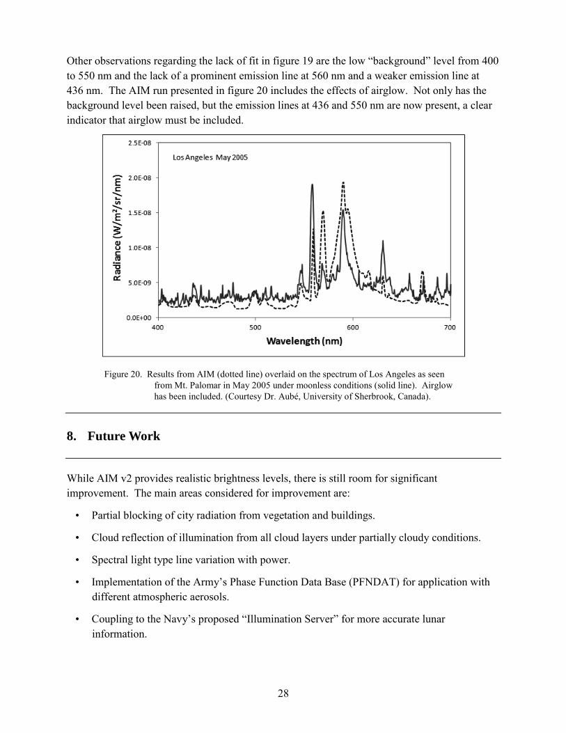
Other observations regarding the lack of fit in figure 19 are the low “background” level from 400 to 550 nm and the lack of a prominent emission line at 560 nm and a weaker emission line at 436 nm. The AIM run presented in figure 20 includes the effects of airglow. Not only has the background level been raised, but the emission lines at 436 and 550 nm are now present, a clear indicator that airglow must be included.

Figure 20. Results from AIM (dotted line) overlaid on the spectrum of Los Angeles as seen from Mt. Palomar in May 2005 under moonless conditions (solid line). Airglow has been included. (Courtesy Dr. Aubé, University of Sherbrook, Canada).

8. Future Work

While AIM v2 provides realistic brightness levels, there is still room for significant improvement. The main areas considered for improvement are:

• Partial blocking of city radiation from vegetation and buildings.

• Cloud reflection of illumination from all cloud layers under partially cloudy conditions.

• Spectral light type line variation with power.

• Implementation of the Army’s Phase Function Data Base (PFNDAT) for application with different atmospheric aerosols.

• Coupling to the Navy’s proposed “Illumination Server” for more accurate lunar information.

29

9. References

1. Practical Guide: Introduction to Light Pollution (PG1), International Dark Sky Association. http://www.darksky.org.

2. Aubé, M.; Franchomme-Fossé, L.; Robert-Staehler, P.; Houle, V. Light Pollution Modelling and Detection in a Heterogeneous Environment: Toward a Night Time Aerosol Optical Depth Retrieval Method. Proceedings from SPIE, Vol. 5890, 2005.

3. Joseph, J. H.; Kaufman,Y. J.; Mekler, Y. Urban light pollution: the effect of atmospheric aerosols on astronomical observations at night. Appl. Opt. 2001, 30, 3047–3058.

4. Garstang, R. H. Model for Artificial Night-Sky Illumination. Publication of the Astronomical Society of the Pacific 1986, 98, 364–375.

5. Shirkey, R. C. An Army Illumination Model (AAIM); ARL-TR-4645; U.S. Army Research Laboratory: White Sands Missile Range, NM, 2008.

6. Kocifaj, M. Light pollution simulations for planar ground-based light sources. Applied Optics 2007.

7. Kocifaj, M. Light-pollution model for cloudy and cloudless night skies with ground-based light sources. Applied Optics 2007, 46, 3013−3022.

8. Garstang, R. H., Light Pollution Modeling, 1991 in Light Pollution, Radio Interference, and Space Debris, ISBN 0-937797-36-8; D.L. Crawford, Bookcrafters, Inc., 56−69.

9. Cinzano, P.; Falchi, F.; Elvidge, C. D. The First World Atlas of the Artificial Night Sky Brightness. Mon. Not. R. Astron. Soc. 2001, 328, 689–707.

10. Luginbuhl, C. B., et al. From The Ground Up I: Light Pollution Sources in Flagstaff, Arizona. Publ. Astron. Soc. Pacific 2009, 121, 185–203.

11. Luginbuhl, C. B., et al. From the Ground Up II: Sky Glow and Near-Ground Artificial Light Propagation in Flagstaff, Arizona. Publ. Astron. Soc. Pacific 2009, 121, 204–212.

12. Walker, M. F. The Effects of Urban Lighting on the Brightness of the Night Sky. Publ. Astron. Soc. Pacific 1977, 89, 405–409.

13. Bertiau, F. C., de Graeve, E. Treanor, P. J. The Artificial Night-Sky Illumination in Italy. Vatican Observatory Publ. 1973, 1, 159−179.

14. Treanor, P. J. A Simple Propagation Law for Artificial Night-Sky Illumination. The Observatory 1973, 93, 117–120.

15. Garstang, R. H. Improved Scattering Formula for Calculations of Artificial Night-Sky Illumination. The Observatory 1984, 104, 196−197.

16. Garstang, R. H. Night-Sky Brightness at Observatories and Sites. Publ. Astron. Soc. Pacific 1989, 101 306–329.

30

17. McClatchey, R. A.; Fenn, R. W.; Selby, J. E. A.; Volz, F. E.;Garing, J. S. Handbook of Optics, ISBN 0-07-047710-8; G. Driscoll and W. Waughan: New York: McGraw-Hill, 1978; p. 14−14.

18. Shettle E. P.; Fenn, R.W. Models for the Aerosols of the Lower Atmosphere and the Effects of Humidity Variations on Their Optical Properties; AFGL-TR-79-0214; Air Force Geophysics Laboratory: Hanscom Air Force Base, MA, 1979.

19. Benn, C. R. and Ellison, S. L. La Palma Night-Sky Brightness; La Palma technical note 115; Roque de los Muchachos Observatory, 2007.

20. Cinzano, P. The Propagation of Light Pollution in Diffusely Urbanized Areas. In Measuring and Modelling Light Pollution; Cinzano, P., Ed.; Mem. Soc. Astron. Italiana: Italy, 2000; pg. 93.

21. Freeman, M. H.; Hull, C. C. Optics, 11th Ed.; ISBN 0 7506 4248 3; Butterworth-Heinemann, 2003; pp 354.

22. Duncan, L. D. and Sauter, D. Natural Illumination under Realistic weather Conditions; ASL-TR-0221-09; Atmospheric Sciences Laboratory: White Sands Missile Range, NM, 1992.

23. Shapiro, R. Solar Radiation Flux Calculations from Standard Meteorological Observations; AFGL-TR-82-0039; Air Force Geophysics Laboratory: Hanscom AFB, MA, 1982.

24. Gouveia, M. J.; Cianciolo, M. E.; Higgins, G. J. Night Vision Goggles Operations Weather Software (NOWS); AFRL-VS-TR-2001-1580; U.S. Air Force Research Laboratory: Hanscom AFB, MA; 2000.

25. Elvidge, C. D.; Keith, D. M.; Tuttle, B. T.; Baugh, K. E. Spectral Identification of Lighting Type and Character. Sensors 2010, 10, 3961−3988.

26. El Paso Electric Co., El Paso, TX. Private communication, 2007.

27. Köppen J. http://astro.u-strasbg.fr/~koppen/divers/AirGlow.html, 1997.

28. Shirkey, R. C. Army Illumination Model v2 User’s Manual; ARL-TR-5705; U.S. Army Research Laboratory: White Sands Missile Range, NM, 2011.

29. van Bochove, A. C. The Computer program ILLUM: Calculation of the Position of Sun and Moon and the Natural Illumination; PHL 1982-13; Physics Laboratory TNO: The Hague, The Netherlands; 1982.

30. Aubé, M. http://www.cegepsherbrooke.qc.ca/~aubema/index.php/Prof/Recherches, Department of Physics, CÉGEP de Sherbrooke, 475 rue Parc, Sherbrooke, QC, Canada.

31

Appendix. Derivation of L cos(θ) = (D – x) sin(z) cos(β) + y sin(z) sin(β) - A cos(z)

Figure A-1. Diagram of the geometric quantities used in AIM.

Consider figure A-1:

d2 = (D – x)2 + y2, (A-1)

L2 = A2 + d2 = A2 + [(D – x)2 + y2], (A-2)

s2 = u2 + L2 – 2 u L cos(θ), (A-3)

also s2 = h2 + c2 = [u cos(z) + A] 2 + c2, (A-4)

cos(β – δ) = cos(β) cos(–δ) – sin(β) sin(–δ) = cos(β) cos(δ) + sin(β) sin(δ), (A-5)

sin(δ) = y/d, (A-6)

cos(δ) = (D – x)/d, (A-7)

c2 = d2 + (u sin(z))2 – 2du sin(z) cos(α), (A-8)

β = α + δ, (A-9)

substituting for d2 and α in (A-8) yields

c2 = (D – x)2 + y2 + u2 sin2(z) – 2d u sin(z) cos(β – δ). (A-10)

32

Using (A-5), (A-6), and (A-7) in (A-10) gives

c2 = (D – x)2 + y2 + u2 sin2(z) – 2 d u sin(z) [cos(β) (D – x)/d + sin(β) y/d],

= (D – x)2 + y2 + u2 sin2(z) – 2 u sin(z) [cos(β) (D – x) + sin(β) y]. (A-11)

Rearranging (A-3) and substituting (A-4) for s2 and (A-2) for L2, we find

u2 = s2 – L2 + 2uL cos(θ) = (u cos(z) + A)2 + c2 – [A2 + (D – x)2 + y2] + 2uLcos(θ), (A-12)

substituting (A-11) into (A-12) and slogging through the math, we find that

u2 = u2[cos2(z) + sin2(z)] + 2u{Acos(z) – sin(z)[(D – x) cos(β) + y sin(β)]} + 2uLcos(θ), (A-13)

and upon rearranging

L cos(θ) = (D – x) sin(z) cos(β) + y sin(z) sin(β)– A cos(z). (A-14)

:QED

33

List of Symbols, Abbreviations, and Acronyms

AIM Army Illumination Model

Ac altocumulus

As altostratus

Cb cumulonimbus

CFL Compact Fluorescent

Ci Cirrus

Cs Cirrostratus

Cu Cumulus

HPS high pressure sodium

IWARS Infantry Warrior Simulation

LED Light Emitting Diode

LOS Line-of-Sight

LPS low pressure sodium

MH metal halide

nL nanolambert

NVG Night Vision Goggles

PFNDAT Phase Function Data Base

Sc stratocumulus

SAA Small Angle Approximation

St stratus

TAWS Target Acquisition Weapons Software

34

No. of Copies Organization 1 PDF Admnstr Defns Techl Info Ctr ATTN DTIC OCP 8725 John J Kingman Rd Ste 0944 Ft Belvoir VA 22060-6218 3 HCs US Army Rsrch Lab Attn RDRL CIO MT Techl Pub Attn RDRL CIO LL Techl Lib Attn IMNE ALC HRR Mail & Records Mgt 2800 Powder Mill Road Adelphi MD 20783-1197 1 HC US Army Rsrch Lab Attn RDRL CI Dr Pellegrino 2800 Powder Mill Road Adelphi MD 20783-1197 1 HC US Army Rsrch Lab Attn RDRL CIE P Clark 2800 Powder Mill Road Adelphi MD 20783-1197 1 HC Atmospheric Environmental Rsrch Inc 1 CD C. Borden 131 Hartwell Avenue Lexington MA 02421-3136 1 HC US Army Rsrch Lab Attn RDRL CIE D D Hoock Building 1622 WSMR NM 88002-5501 1 HC US Army Rsrch Lab Attn RDRL CIE M D Knapp Building 1622 WSMR NM 88002-5501 2 HCs US Army Rsrch Lab 1 CD Attn RDRL CI M R Shirkey Building 1622 WSMR NM 88002-5501 1 HC Naval Research Laboratory 1 CD Marine Meteorology Division A Goroch 7 Grace Hopper Ave Monterey CA 93943

No. of Copies Organization 1 HC Northrop Grumman 1 CD M Gouveia 100 Brickstone Square Andover MA 01810 1 HC Atmospheric Environmental Research Inc 1 CD G Seeley 131 Hartwell Avenue Lexington MA 02421-3136 1 HC Science Applications 1 CD International Corporation L Delgado 731 Lakepointe Centre Drive O’Fallon IL 62269-3064 3 HCs US Army Natick Soldier 1 CD RD&E Center Attn AMSRD NSR TS M B Auer 15 Kansas Street Natick MA 01760-5056 1 HC Director USA Tradoc Analysis Center 1 CD Attn ATRC WMM D Ohman WSMR NM 88002-5502 1 HC Aerodyne Research Inc. 1 CD F Iannarilli 45 Manning Road Billerica MA 01821 1 HC Département de physique

CÉGEP de Sherbrooke M Aubé 475 rue du CÉGEP Sherbrooke (Québec) Canada J1E 4K1

1 HC U.S. Army RDECOM CERDEC Night Vision and Electronic Sensors Directorate R Littleton 10221 Burbeck Rd

Fort Belvoir VA 22060-5806

1 HC US Army Rsrch Lab 1 CD Attn RDRL CI M D Tofsted Building 1622 WSMR NM 88002-5501

35

No. of Copies Organization

1 HC US Army Rsrch Lab 1 CD Attn RDRL CI M S O’Brien Building 1622 WSMR NM 88002-5501

1 HC US Army Rsrch Lab Attn RDRL CI M E Measure Building 1622 WSMR NM 88002-5501 1 HC Blue Storm Technologies 1 CD M Lockhart 8605 Cross View Fairfax Station VA 22039-3358 1 HC Science Applications 1 CD International Corporation R Rensing 91 Hartwell Ave Lexington MA 02421 1 HC Union College L Relyea Dept of Sociology 807 Union St Schenectady NY 12308 1 HC Met Office W Lewis FitzRoy Rd Exeter

Devon EX1 3PB United Kingdom Total: 42 (1 PDF, 28 HCs, 13 CDs)

36

INTENTIONALLY LEFT BLANK.