Embed Size (px)
Citation preview
SLAC-PUB-10150
October 2003
Submitted to Physics in Perspective *Work supported by Department of Energy contract DE-AC03-76SF00515.
Tau Discovery
THE DISCOVERY OF THE TAU LEPTON AND THE CHANGES IN ELEMENTARY PARTICLE PHYSICS IN 40
YEARS
Martin L. Perl
Stanford Linear Accelerator Center and
Stanford University, Stanford, CA 94309
Phone: 650-926-4286
Fax: 650-926-4001
Email: [email protected]
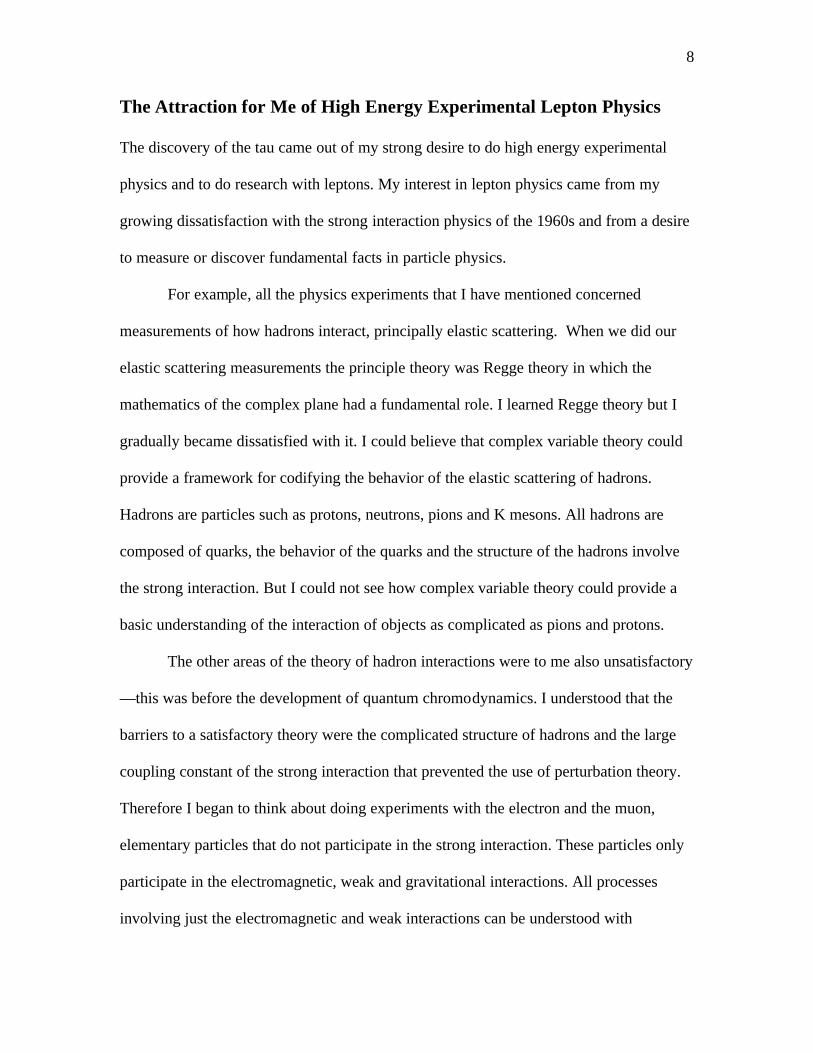
Introduction
This is a history of my discovery of the tau lepton in the 1970s for which I was awarded
the Nobel Prize in Physics. I have previously described some aspects of the discovery. In
1996 in my collection of papers entitled, “Reflections on Experimental Science,”1 I gave
a straightforward account of the experimental method and the physics involved in the
discovery as an introduction to the collection. In a 2002 paper2 written with Mary A.
Meyer published in the journal Theoria et Historia Scientiarum I used the story of the
discovery to outline my thoughts on the practice of experimental science. That 2002
paper was written primarily for young women and men who are beginning their lives in
science and it was based on a lecture given at Los Alamos National Laboratory. Some of
the historical material in this paper has appeared in those two earlier papers.
This history of the tau discovery has three goals. First, I want to give the history
of the discovery. Second, I want to give a general picture of the high energy physics
world of thirty to forty years ago. It was very different from today's world of high energy

2
physics. Third, and particularly important to me, I want to try to describe the differences
between today’s world of high energy physics and that of forty years ago. Are there
intrinsic differences—not just differences in the size of the community and in the size and
complexity of the experiments? Has our greatly increased knowledge and understanding
of elementary particles and forces changed the way we do research in particle physics?
Today there seems to be more speculative work in elementary particle theory than there
was forty years ago. Is this true? Is more speculative theory good or bad or irrelevant to
the progress of particle physics? I will explore and discuss such questions as I recount the
discovery history.
I will interrupt the narrative from time to time to present my observations on what
I believe have been the changes in the world of high energy physics over the past forty
years. I will put these observations in italics.
My Education and Early Work in Engineering
It has been a long and indirect voyage that led me to work in lepton physics and led to the
discovery of the tau lepton. As a boy I was what used to be called ‘mechanically
inclined’. I loved building things out of scrap wood, I loved working with Erector Sets,
and I did some home chemistry. I was very good in high school mathematics and physics.
When I graduated from the Brooklyn, New York, academic high school, James Madison,
in 1939, I won the physics medal. But neither I nor my parents knew that one could have
a career in physics so the next choice was engineering. I enrolled in the Polytechnic
Institute of Brooklyn, now Polytechnic University, and began studying chemical
engineering. There were two reasons for choosing chemical engineering. Chemistry was

3
a very exciting field in the late 1930s and early 1940s. There would always be a good job
in chemical engineering.
My studies were interrupted by World War II. When the war ended, I returned to
the Polytechnic Institute and received a summa cum laude bachelor’s degree in chemical
engineering in 1948. The skills and knowledge I acquired at the Polytechnic Institute
have been crucial in all my experimental work, including the use of strength-of-materials
principles in equipment design, machine shop practice, and engineering drawing.
Upon graduation, I joined the General Electric Company. After a year in an
advanced engineering training program, I settled in Schenectady, New York, working as
a chemical engineer in a group in the electron tube production factory. The group’s
purpose was to troubleshoot production problems, to improve production processes, and
occasionally to do a little development work. We were not a fancy R&D office. I was
happy as an engineer. I liked the combination of working with my hands, of designing
equipment, of carrying out tests, and of being connected with science.
For my job I had to learn how electron vacuum tubes worked, so I took a few
courses at Union College in Schenectady, specifically atomic physics and advanced
calculus. I got to know a wonderful physics professor, Vladimir Rojansky. One day he
said to me, “Martin, what you are interested in is called physics—not chemistry, not
engineering!” At the age of 23, I finally decided to begin the study of physics. I enrolled
at Columbia University in New York City.

4
Going Into Physics
Just as the Polytechnic Institute was crucial in my learning how to do engineering, just as
Union College and Vladimir Rojanskya were crucial in my choosing physics, so
Columbia University and my thesis advisor, I. I. Rabi, were crucial in my learning how to
do experimental physics. I entered the physics doctoral program in Columbia University
in the autumn of 1950. Looking back, it seems amazing that I was admitted with just a
bachelor’s degree in chemical engineering. True, I had a summa cum laude bachelor’s
degree, but I had taken only two courses in physics: one year of elementary physics and a
half-year of atomic physics. It would be much harder to do this today.
Graduate study in physics was primitive in the 1950s, compared to today’s
standards. Most of us did not study quantum mechanics until the second year; the first
year was completely devoted to classical physics. The most advanced quantum
mechanics we ever studied was a little bit in Heitler,3 and we were not expected to be
able to do calculations in quantum electrodynamics. We did not know how to use
Feynman diagrams.
This brings me to one of the differences between the graduate school
physics of 50 years ago and today. Less was known and we had less to
study. I don’t think that learning so much less in graduate school was a
complete disadvantage. It gave all the students more time to think about
physics outside their specialty. In particular, experimenters had more time
to learn all sorts of experimental techniques.
a Vladimir Rojansky may be known to some of the older readers through his textbooks on
electromagnetism and on quantum mechanics.

5
I undertook for my doctoral research the problem of using the atomic-beam
resonance method to measure the quadrupole moment of the sodium nucleus.4 (The
atomic-beam resonance method was invented by Rabi, for which he received a Nobel
Prize in 1944.) This quadrupole measurement had to be made using an excited atomic
state, and Rabi had found a way to do this. My experimental apparatus was boldly
mechanical, with a brass vacuum chamber, a physical beam of sodium atoms, submarine
storage batteries to power the magnets—and, in the beginning of the experiment, a wall
galvanometer to measure the beam current. I developed much of my style in experimental
science during this thesis experiment. When designing the experiment and when thinking
about the physics, the mechanical view is always dominant in my mind. More
importantly, my thinking about elementary particles is physical and mechanical. In the
basic production process for tau leptons
e+ + e− → τ+ + τ− .
I see the positron, e+, and electron, e−, as tiny particles that collide and annihilate one
another. I see a tiny cloud of energy formed which we technically call a virtual photon,
γvirtual. Then I see that energy cloud change into two tiny particles of new matter—a
positive tau lepton, τ+, and a negative tau lepton, τ−.
My thesis was in atomic physics, but it was Rabi who always emphasized the
importance of working on a fundamental problem, and it was Rabi who sent me into
elementary particle physics. It would have been natural for me to continue in atomic
physics, but he preached particle physics to me as the coming field and in 1955, the year I
received my Ph. D., it indeed was the coming field. I went to the Physics Department of
the University of Michigan as an Instructor to teach and to do research in particle physics.
Yes, in the late 1950s, there were still instructors in physics departments.

6
High-Energy Physics at the Cosmotron and the Bevatron
At Michigan, I made the change from atomic physics to high-energy physics. I first
worked in bubble chamber physics with Donald Glaser, the inventor of the bubble
chamber. We carried out our bubble chamber experiments at the Cosmotron of the
Brookhaven National Laboratory. But I wanted to be on my own. When the Russians
flew SPUTNIK in 1957, I saw the opportunity and jointly with my colleague, Lawrence
W. Jones, obtained research support from the Office of Naval Research. We began our
own research program using first the now-forgotten luminescent chamber.5 A luminescent
chamber consists of one or more pieces of sodium iodide scintillator. We photographed
and recorded the tracks of charged particles in the sodium iodide crystals using primitive
electron tubes that intensified the light coming from the track. In 1960, at the Bevatron of
the Lawrence Berkeley Laboratory, we carried out a somewhat primitive measurement of
the elastic scattering of high-energy pions colliding with protons.6
But the newly invented optical spark chamber was a much better device for
determining the paths of charged particles. Jones and I, using spark chambers, carried out
at the Bevatron in the early 1960s, a definitive set of measurements on the elastic
scattering of pions on protons.7
From the late 1960s to the early 1970s Michael Kreisler, Michael Longo, and I
carried out some experiments on the high energy scattering of neutrons on protons8 using
optical spark chambers, one of them being a special thick-plate spark chamber where the
scattered neutron was detected by its interaction in the thick plates. By this time I was at
the Stanford Linear Accelerator Center.

7
Thus, in fifteen years, a handful of colleagues and I worked on about a dozen
experiments using all sorts of experimental techniques in elementary particle physics—
scintillation counters, bubble chambers, luminescent chambers, spark chambers,
coincidence and counting electronics, scanning and measuring tables for bubble chamber
and spark chamber pictures. We also used the mainframe computers of the early 1960s
with the programs and data usually on punch cards.
This illustrates several major differences between the high energy physics
experiments of forty years ago and today. Forty years ago, one could build
the apparatus in a year, except for bubble chambers, frequently using
parts from previous experiments. And except for bubble chambers, the
time spent acquiring data at an accelerator was often of the order of a
month. We were not smarter than today’s experimenters and we did not
work harder. The experimental methods that we knew were much simpler
and we could easily build anything we needed.
It was therefore relatively easy to think about trying to measure something
better or something new, then to build the apparatus, and then within
several years to have the results. This gave the experimenter a wonderful
freedom to try all sorts of new directions and new ideas, in contrast to
today’s high energy experiments that are typically very large, very
complicated, and may take a decade to build. Of course, these modern
experiments provide data for hundreds of different measurements and
studies, and so are, in some ways, the equivalent of hundreds of
experiments of forty years ago. But the experimental possibility of quick
changes is mostly gone. There is nothing we can do about this; the easy
elementary particle questions were answered thirty and forty years ago.
8
The Attraction for Me of High Energy Experimental Lepton Physics
The discovery of the tau came out of my strong desire to do high energy experimental
physics and to do research with leptons. My interest in lepton physics came from my
growing dissatisfaction with the strong interaction physics of the 1960s and from a desire
to measure or discover fundamental facts in particle physics.
For example, all the physics experiments that I have mentioned concerned
measurements of how hadrons interact, principally elastic scattering. When we did our
elastic scattering measurements the principle theory was Regge theory in which the
mathematics of the complex plane had a fundamental role. I learned Regge theory but I
gradually became dissatisfied with it. I could believe that complex variable theory could
provide a framework for codifying the behavior of the elastic scattering of hadrons.
Hadrons are particles such as protons, neutrons, pions and K mesons. All hadrons are
composed of quarks, the behavior of the quarks and the structure of the hadrons involve
the strong interaction. But I could not see how complex variable theory could provide a
basic understanding of the interaction of objects as complicated as pions and protons.
The other areas of the theory of hadron interactions were to me also unsatisfactory
—this was before the development of quantum chromodynamics. I understood that the
barriers to a satisfactory theory were the complicated structure of hadrons and the large
coupling constant of the strong interaction that prevented the use of perturbation theory.
Therefore I began to think about doing experiments with the electron and the muon,
elementary particles that do not participate in the strong interaction. These particles only
participate in the electromagnetic, weak and gravitational interactions. All processes
involving just the electromagnetic and weak interactions can be understood with

9
perturbation theory calculations, and with enough patience. The effect of the gravitational
force on the interactions of elementary particles is very small, too small to take into
account.
There were two puzzles about the properties of the electron, e, and the muon, µ, in
the 1960s and fundamentally these puzzles remain today, built into the so-called standard
model of elementary particle physics. First, as shown in Table 1, the properties with
respect to particle interactions are the same for the electron and the muon, but the muon
is 208 times heavier. Why?
The second puzzle has to do with the instability of the muon. One might expect
the muon to decay through the process
µ− → e− + γ (1)
Here, γ means a photon, and the expectation would be that the γ carries off the excess
energy produced by the difference between the muon mass and the electron mass. (An
analogous decay equation can be written for the positive muon but to save space I will
usually write the decay process for only the negative lepton.) However the muon decays
to an electron by a more complicated process,
µ− → e− + eν + νµ (2)
in which an electron antineutrino ( eν ) and a muon neutrino (νµ) are produced. The muon
lifetime is 2.2×10⁻⁶ seconds due to this more complicated decay process. The simpler
decay process using the photon, Eq. 1, has never been seen and the measured upper limit
on its probability compared to the more complicated process, Eq. 2, is about 10-11.9 Our
present understanding of the extreme suppression of the photon decay mode is that there

10
is an intrinsic difference between the nature of the electron and the nature of the muon.
Therefore the only substantial decay process is that depicted by Eq. 2 in which, when a
muon decays, the intrinsic nature of the muon is carried on the muon neutrino and the
production of an electron is compensated for by the simultaneous production of an
antielectron neutrino.
SLAC and Leptons
In 1963, the opportunity arose to think seriously about high-energy experiments on
charged leptons when Wolfgang K. H. Panofsky and Joseph Ballam offered me a position
at the yet-to-be-built Stanford Linear Accelerator Center (SLAC). Here was a laboratory
that would have primary electron beams: a laboratory at which one could easily obtain a
good muon beam, and a laboratory at which one could easily obtain a good photon beam
for producing lepton pairs. Furthermore, on the Stanford campus at the High Energy
Physics Laboratory, the Princeton-Stanford e− e− storage ring was operating.
When I arrived at SLAC in 1963, I began to plan various attacks on, and
investigations of, the electron-muon problem. Although the linear accelerator would not
begin operation until 1966, my colleagues and I began to design and build experimental
equipment. My proposed attacks and investigations were of two classes. In one class, I
proposed to look for unknown differences between the electron and the muon, the only
known differences being the mass difference and the observation that the decay reaction
µ → e + γ does not occur. The other class of proposed attacks and investigations was
based on my speculation that there might be more leptons similar to the electron and the

11
muon, unknown heavier charged leptons. I dreamed that if we could find a new lepton,
the properties of the new lepton might teach us the secret of the electron-muon puzzle.
My first attack used an obvious idea.10 An intense photon (γ) beam could be made at
SLAC using the reactions
e− + nucleus → γ +. . . .
The photons so produced could then interact with another nucleus to produce a pair of
charged particles: x+ and x−,
γ + nucleus → x+ + x− + . . .
Any pair of charged particles could be produced if the γ had enough energy. My hope
was that we would find a new x particle, perhaps a new charged lepton somehow related
to the electron or muon, a vague hope by the standards of our knowledge of elementary
particle physics today. We were certainly naive in the 1960s. We didn’t find any new
leptons or any new particles of any kind;10 as we now know, there were no new particles
to find given the experimental limitations of this search experiment. The search used the
pair-production calculations of Y. S. Tsai and V. Whitis.11
Studies of Muon-Proton Inelastic Scattering
Although this first attempt to penetrate the mysteries of the electron and muon failed, we
were already preparing to study muon-proton inelastic scattering,
µ−+ p → µ− + hadrons
to compare it with electron–proton inelastic scattering,
e− + p → e− + hadrons.

12
Extensive studies of e–p inelastic scattering were planned at SLAC. Indeed, some of
those studies, which revealed the presence of quarks in hadrons, led to the awarding of
the 1990 Nobel Physics Prize to Jerome Friedman, Henry Kendall, and Richard Taylor.
My hope was that we would find a difference between the µ and e other than the
differences of mass and lepton type. For example, I speculated that the muon might have
a special interaction with hadrons not possessed by the electron.12,13
My colleagues and I measured the differential cross sections for inelastic
scattering of muons on protons, and then compared the µ–p cross sections with the
corresponding e–p cross sections.13 We were looking for a difference in magnitude or a
difference in behavior of the cross sections. These differences could come from a new
nonelectromagnetic interaction between the µ and hadrons or from the µ’s not being a
point particle. However we found no significant deviation.14,15
Other experimenters studied the differential cross section for µ–p elastic
scattering and compared it with e–p elastic scattering but statistically significant
differences between µ–p and e–p cross sections could not be found in either the elastic or
inelastic cases.16 Furthermore, there were systematic errors of the order of 5% or 10% in
comparing µ–p and e–p cross sections because the techniques used were so different.
Experimental science is a craft and an art, and part of the art is knowing
when to end a fruitless experiment. There is a danger of becoming
obsessed with an experiment even if it goes nowhere. At some point,
you’ve got to say, “I really don’t know how to improve this.” I avoided
obsession and gave up on the scattering experiment. That turned out to be
a good decision because modern experiments have shown that these
scattering experiments do not illuminate any differences between the
electron and the muon beyond the mass difference.

13
Heavy Leptons in the 1960s
While building the apparatus using our muon-proton inelastic scattering experiment, and
during the first operation of that experiment, I was thinking of another way to look for
new charged leptons, L, using the reaction
e+ + e− → L+ + L− .
Before turning to this third attack on the electron-muon problem, I will describe the
general thinking in the 1960s about the possible existence and types of new leptons. By
the beginning of the 1960s, papers had been written on the possibility of the existence of
charged leptons more massive than the e and µ, usually called heavy leptons. I remember
reading the 1963–1964 papers of Ya B. Zel’dovich,17 of E. M. Lipmanov,18 and of L. B.
Okun.19 Since the particle generation concept was not yet an axiom of our field, older
models of particle relationships were used. For example, if one thought that there might
be an electromagnetic excited state e* of the e20, then the proper search method was
e− + nucleon → e−* + . . . , e−* → e− + γ.
If one thought that the µ belonged to three-member family consisting of a µ, νµ, and a
heavier version of the µ, µ', then the proper search method was
νµ + nucleon → µ'−+ . . . .
By the second half of the 1960s, the concept had been developed of a heavy
lepton L and its neutrino νL forming an L, νL pair. Thus, in a paper written in 1968, K. W.
Rothe and A. M. Wolsky 21 discussed the lower mass limit on such a lepton set by its
absence in K meson decays. They also discussed the decay of such a lepton into the
modes
L- → e- + eν + νL, L- → µ- + µν + νL, L- → p− + νL .

14
This brings me to the question I raised in the Introduction: is there more
and broader speculation these days in particle physics theory than forty
years ago? Judging by the various ideas of forty years ago about possible
types of leptons, we were rather timid about speculations. There was a
fear of being thought unsound. There was reluctance to stray too far from
what was known. Today the only limit to theoretical speculations about
particle physics is that the mathematics be correct and that there be no
obvious conflict with measured properties of particles and reactions. One
example is string theory with all its different forms and extensions.
Another example is the recent, tremendous amount of interweaving of
particle physics with astrophysics and cosmology. I think this is a good
change. It can stimulate the experimenter to go in new directions, but the
experimenter must be cautious as to how she or he uses time. If possibly
relevant data have already been produced, then it may be relatively fast to
test the speculation against the data. But if a new experiment must be built
to test the speculation, that is another story.
Electron-Positron Colliders
The obvious and most general way to try to produce and detect new charged leptons was
to use an electron-positron collider for the production process
e+ + e− → L+ + L− .
The principle of operations of a circular electron-positron collider is shown in figure 1. A
bunch of electrons (closed circles) and a bunch of positrons (open circles) circulate in
opposite directions in a circular ring consisting of an evacuated pipe. The cross-sectional
size of the pipe is much smaller than the diameter of the ring. For example, in the SPEAR
collider (figure 2) the cross-sectional size of the pipe is of the order of 10 centimeters and
the diameter of the ring is about 60 meters. As the bunches circulate they pass through
each other in two places called interaction points. Almost all of the electrons and

15
positrons pass by each other but occasionally an electron and a positron collide and
interact, producing new particles.
The construction and operation of electron-positron colliders began in the
1960s.22 By September 1967 at the Sixth International Conference on High Energy
Accelerators, F. T. Howard23 was able to list quite a few electron-positron colliders. The
pioneer 500-MeV ADA collider was already operating at Frascati in the early 1960s.
Also at Frascati, ADONE was under construction. The 1-GeV ACO at Orsay and 1.4-
GeV VEPP-2 at Novosibirsk were in operation. The 6-GeV CEA Collider at Cambridge
was being tested, and colliders had been proposed at DESY and SLAC.24
The 1964 SLAC proposal by David Ritson, et al.24 had already discussed the
reaction
e+ + e− → x+ + x− .
Of course, x might be a charged lepton. This proposal did not lead directly to the
construction of an e+e– collider at SLAC because we could not get the funding. About
five years later—with the steadfast support of the SLAC director, Wolfgang Panofsky,
and with a design and construction team led by Burton Richter—construction of the
SPEAR e+e– collider was begun at SLAC.
The Sequential Lepton Model
It was this 1964 proposal and the 1961 seminal paper of N. Cabibbo and R. Gatto25 that
focused my thinking on new charged lepton searches using an e+e– collider. As we
carried out the experiments described previously, I kept looking for a model for new
leptons—a model that would lead to definitive colliding beam searches, while remaining
reasonably general. Helped by discussions with colleagues such as Paul Tsai and Gary

16
Feldman, I came to what I later called the sequential lepton model. I thought of a
sequence of pairs
e− νe
µ− νµ
L− νL
L'− νL',
each pair having a unique lepton type. I usually thought about the leptons as being point
Dirac particles. Of course, the assumptions of unique lepton type and point particle nature
were not crucial, but I liked the simplicity. After all, I had turned to lepton physics in the
early 1960s in a search for simple physics. The idea was to look for
e+ + e− → L+ + L−,
with
L+ → e+ + undetected neutrinos carrying off energy
L− → µ− + undetected neutrinos carrying off energy,
or
L+ → µ++ undetected neutrinos carrying off energy
L− → e− + undetected neutrinos carrying off energy.
This search method had many attractive features:
• If the L was a point particle, we could search up to an L mass almost equal to the
beam energy, if we had enough luminosity.
• The appearance of an e+µ− or e−µ+ event with missing energy would be dramatic.
• The apparatus we proposed to use to detect the L decays would be very poor in
identifying types of charged particles (certainly by today’s standards), but the easiest
particles to identify were the e and the µ.

17
• Perturbation calculations using weak interaction theory predicted that the L would
have the weak decays
L− → νL + e− + eν
L− → νL + µ− + µν ,
with corresponding decays for the L+. The decay rate was easily calculated.
My ability to make detailed calculations on how the hypothetical L lepton
would decay shows the major change that has occurred in the ability of a
busy experimenter to make detailed calculations from first principles on
her or his experiment. Suppose today I wanted to make analogous
calculations on the decays of a particle predicted in a string theory. A
kindly string theorist could set up the final equations for me but it would
be impossible for me to do the calculations from first principles. Many
areas of particle theory are now too advanced and too complicated for the
amateur theorist. First-principle calculations can only be done by those
who are devoted full time to theory. This is a sad change but there is
nothing that can be done; many areas of theory require full time for
understanding and use. Meanwhile the experimenter is busier than ever
building or operating the experiment or analyzing the data.
I incorporated this search method in our 1971 SLAC-LBL proposal to use the not-
yet-completed SPEAR e+e− storage ring.26 My thinking about sequential leptons and this
search method was greatly helped by a 1971 seminal paper of Paul Tsai27 providing
detailed calculations on how a sequential lepton would decay. Thacker and Sakurai28 also
published a paper on the theory of sequential lepton decays, but it is not as
comprehensive as the work of Tsai.

18
The Beginnings of the Sequential Lepton Search at SPEAR
After numerous funding delays, a group led by Burton Richter and John Rees of SLAC
Group C began to build the SPEAR e+e−collider at the end of the 1960s (figure 2). Gary
Feldman and I, along with our Group E, joined with their Group C and a Lawrence
Berkeley Laboratory group led by William Chinowsky, Gerson Goldhaber, and George
Trilling to build a SLAC-LBL particle detector for use at SPEAR. In 1971 we submitted
the SLAC-LBL proposal.26
The SLAC-LBL detector (figures 3 and 4) was one of the first of the large solid
angle, general-purpose detectors. The purpose of a general-purpose detector is to detect
the type and vector momentum of most of the particles coming from a reaction taking
place at the center of the detector. The goal is to detect and identify electrons, muons,
protons, pions, and K mesons.
Large solid angle, general-purpose detectors and other types of large
detectors such as neutrino detectors have become the norm in
experimental particle physics. These detectors are necessary to obtain the
complicated and often subtle data in modern experiments. But large
detectors have come at a human cost. It is no longer possible for a few
people to build and operate such detectors. Hence there are often
hundreds of experimenters in a typical group and the new very large and
complicated detectors require groups with more than a thousand
members. Of course such detectors produce tremendous amounts of data.
The contents of the proposal26 consisted of five sections (Introduction, Boson
Form Factors, Baryon Form Factors, Inelastic Reactions, Search for Heavy Leptons),
followed by figure captions, references, and the Supplement. The heavy lepton search
was left for last and allotted just three pages, because to most others it seemed a remote

19
dream. But the three pages did contain the essential idea of searching for heavy leptons
using eµ events.
I wanted to include a lot more about heavy leptons and the e–µ problem, but my
colleagues thought that would unbalance the proposal. We compromised on a 10-page
supplement titled, “Supplement to Proposal SP-2 on Searches for Heavy Leptons and
Anomalous Lepton-Hadron Interactions,” which began as follows:
“While the detector is being used to study hadronic production processes it is possible
to simultaneously collect data relevant to the following questions:
• Are there charged leptons with masses greater than that of the muon?
• Are there anomalous interactions between the charged leptons and the
hadrons?”
Though my first interest was to look for heavy leptons, I still had my old interest of
looking for an anomalous lepton interaction, the idea that led to the study of
muon-proton inelastic scattering.
While SPEAR and the SLAC-LBL detector were being built, lepton searches
were being carried out at the ADONE e+e− storage ring by two groups of experimenters in
electron-positron annihilation physics: one group reported in 1970, Alles-Borelli, et al.,29
and then in 1973, Bernardini, et al..30 In the later paper, they searched up to a mass of
about 1 GeV for a conventional heavy lepton and up to about 1.4 GeV for a heavy lepton
with decays restricted to leptonic modes. The other group of experimenters in electron-
positron annihilation physics was led by Shuji Orito and Marcello Conversi. Their search
region also extended to masses of about 1 GeV.31 No heavy leptons were found in these
searches because, as we now know, there are no heavy leptons in the mass range between
the muon and the tau.

20
The SPEAR electron-positron collider began operation in 1973. Eventually
SPEAR obtained a total energy of about 8 GeV, but in the first few years, the maximum
energy with useful luminosity was 4.8 GeV. We began operating the SLAC-LBL
experiment in 1973 in the form shown in figure 3. The SLAC-LBL detector was one of
the first large, solid-angle, general purpose detectors built for colliding beams. The use of
large, solid-angle particle tracking and the use of large, solid-angle particle identification
systems is obvious now, but it was not obvious thirty years ago. The electron detection
system used lead-scintillator sandwich counters built by our Berkeley colleagues. The
muon detection system was also crude, using the iron flux return which was only 1.7
absorption lengths thick.
The SLAC-LBL detector contained two important elements now used in all
modern particle detectors. First, we made extensive use of transistor electronics. The
reliability, relatively small size, and relatively low cost of transistor electronics allowed a
relatively fine division of the detector into many particle-detecting channels. The SLAC-
LBL detector had hundreds of channels; modern large detectors may have hundreds of
thousands of particle detecting channels.
The second important element was the extensive use of computers. The data were
recorded on magnetic tape by a mainframe computer and monitoring of the detector
performance was also done in real time using the computer. Of course, the processing of
the raw data and the analysis of the processed data were also done by computer.
The tremendous advances in electronics and computer computation in the
past thirty years have been crucial to the tremendous experimental
progress in elementary particle physics. However this great good has led
to deep change in the relationships between physicists and the

21
development of new technology. There was a time when physicists were
the inventors and innovators for most of the technology that they used.
And if necessary they could build any piece of equipment they needed,
even that involving the newest technology. But this is no longer true for
electronics and computers. The use of electronics and computers in
civilian, business and military areas now drives the major advances in the
electronics and computer industry. Elementary particle experimenters can
sometimes purchase variations of standard electronics and computer
products, but mostly they purchase the standard products.
First Evidence for a New Lepton
In June 1975, I gave the first international talk on the e–µ events at the 1975 Summer
School of the Canadian Institute for Particle Physics.32 My purpose was to show that (1)
we had good evidence for e–µ events and (2) to discuss possible sources of the e–µ
events: heavy leptons, heavy mesons, or intermediate bosons. The largest, single energy
data sample (table 2) was at 4.8 GeV, the highest energy at which we could then run
SPEAR. The 24 e–µ events were the strongest evidence at that time for the tau. One of
the cornerstones of this claim was an informal analysis carried out by Jasper Kirkby, who
was then at Stanford University and at SLAC. He showed me that by just using the
numbers in table 2, we could calculate the probabilities for hadron misidentification in
this class of events. There were not enough e-h, µ-h, and h-h events to explain away the
24 e–µ events. The misidentification probabilities determined from three-or-more-prong
hadronic events and other considerations are given in table 3. Compared to present
experimental techniques, the Ph → e and Ph→ µ misidentification probabilities of about
0.2 are enormous, but I could still show that the 24 e–µ events could not be explained
22
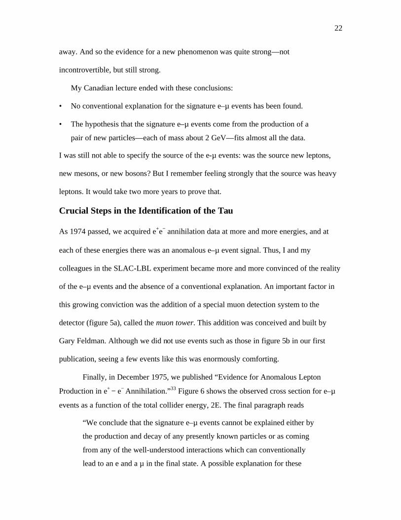
away. And so the evidence for a new phenomenon was quite strong—not
incontrovertible, but still strong.
My Canadian lecture ended with these conclusions:
• No conventional explanation for the signature e–µ events has been found.
• The hypothesis that the signature e–µ events come from the production of a
pair of new particles—each of mass about 2 GeV—fits almost all the data.
I was still not able to specify the source of the e-µ events: was the source new leptons,
new mesons, or new bosons? But I remember feeling strongly that the source was heavy
leptons. It would take two more years to prove that.
Crucial Steps in the Identification of the Tau
As 1974 passed, we acquired e+e− annihilation data at more and more energies, and at
each of these energies there was an anomalous e–µ event signal. Thus, I and my
colleagues in the SLAC-LBL experiment became more and more convinced of the reality
of the e–µ events and the absence of a conventional explanation. An important factor in
this growing conviction was the addition of a special muon detection system to the
detector (figure 5a), called the muon tower. This addition was conceived and built by
Gary Feldman. Although we did not use events such as those in figure 5b in our first
publication, seeing a few events like this was enormously comforting.
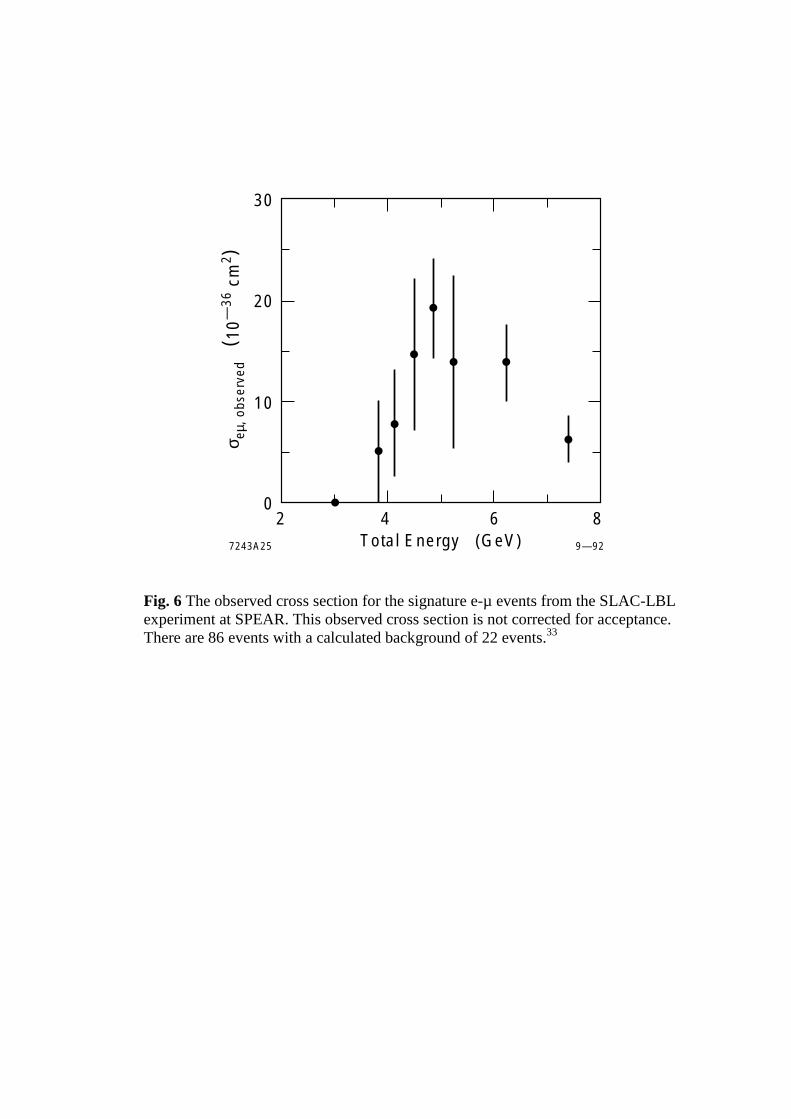
Finally, in December 1975, we published “Evidence for Anomalous Lepton
Production in e+ − e− Annihilation.”33 Figure 6 shows the observed cross section for e–µ
events as a function of the total collider energy, 2E. The final paragraph reads
“We conclude that the signature e–µ events cannot be explained either by
the production and decay of any presently known particles or as coming
from any of the well-understood interactions which can conventionally
lead to an e and a µ in the final state. A possible explanation for these

23
events is the production and decay of a pair of new particles, each having
a mass in the range of 1.6 to 2.0 GeV/c2 .”33
We were not yet prepared to claim that we had found a new charged lepton, but we were
prepared to claim that we had found something new. To accentuate our uncertainty I
denoted the new particle by U for “unknown” in some of our 1975–1977 papers. The
name tau, τ, was suggested by Petros Rapidis, who was then a graduate student and
worked with me in the early 1970s. The letter τ is from the Greek triton for third—the
third charged lepton. Thus in 1975, twelve years after we began our lepton physics
studies at SLAC, these studies finally bore fruit. But we still had to convince the world
that the e–µ events were significant, and we had to convince ourselves that the e–µ events
came from the decay of a pair of heavy leptons.
The success of the search illustrates some basic principles for searches for
new particles. These principles have remained the same over all these
years. First, we had cast a wide net in studying the electron-muon
problem: an attempt to photoproduce new leptons, experimental
comparisons of muon-proton inelastic scattering with electron-proton
inelastic scattering, and the use of the general reaction e+ + e– → L+ + L–
to try to produce a heavy lepton. Second, a new technology, the electron-
positron collider, was available to carry out the L+ L– production. Third,
we had a good way to detect the L+ L– production, namely the search for
e-µ events without photons. Fourth, I had smart, resourceful, and patient
research companions. I think these are the elements that should be present
in speculative experimental work: a broad general plan, specific research
methods, new technology, and first-class research companions. Of course,
the element of luck will in the end be dominant. We had two great pieces
of luck. First, there was a heavy lepton within the energy range of the
SPEAR collider. Second, the SLAC-LBL experimental apparatus was good
enough to enable us to identify the e–µ events and prove their existence.

24
Is It a Lepton?
Our first publication was followed by several years of confusion and uncertainty about
the validity of our data and its interpretation. It is hard to explain this confusion decades
later when we know that τ+τ-pair production is 20% of the e+e– annihilation cross section
below the Z°, when τ+τ- pair events stand out so clearly at the Z°.
There were several reasons for the uncertainties of that period. It was hard to
believe that both a new meson, the D charm meson, and a new lepton, the tau, would be
found in the same narrow range of masses. The D mass is about 1.87 GeV/c2 and the tau
mass is about 1.77 GeV/c2. Also, while the existence of the fourth quark, the charm
quark, c, that comprises most of the mass of the D meson, was required by theory, there
was no such requirement for a third charged lepton, so there were claims that the e-µ
events were from the decays of pairs of D mesons. There were also claims that other
predicted decay modes of tau pairs, such as e–hadron and µ–hadron events, could not be
found. Indeed, finding such events was just at the limit of the particle identification
capability of the detectors of the mid-1970s.
Perhaps the greatest impediment to the acceptance of the tau as the third charged
lepton was that there was no other evidence for a third particle generation. Two
generations of quarks and leptons—u, d, e–, νe and c, s, µ–, νµ—seemed acceptable, a
kind of doubling of particles. But why three generations? To this day, this question has
no answer. It was a difficult time. Rumors kept arriving of definitive evidence against the
τ: e–µ events not seen, the expected decay modes not seen, theoretical problems with
momentum spectra or angular distribution. With colleagues such as Gary Feldman, I went
over our data again and again. Had we gone wrong somewhere in our analysis of the

25
data? Clearly, other tau pair decay modes had to be found. Assuming the tau to be a
charged lepton with conventional weak interactions, simple and very general theory
predicted the branching fractions
B(τ−→ ντ + e- + ν e ) = 20%
B(τ−→ ντ + µ- + ν µ ) = 20%
B(τ−→ ντ + hadrons) = 60%.
Experimenters therefore should be able to find the decay sequences
e+ + e− → τ+ + τ−
τ+ → ν τ + µ++νµ
τ− →ντ + hadrons.
This sequence would lead to anomalous muon events
e+ + e− →µ± + hadrons + missing energy,
Analogously there should be anomalous electron events
e+ + e− → e± + hadrons + missing energy.
Anomalous Muon Events, Anomalous Electron Events, and More
Evidence for the Tau
The first advance beyond the e–µ events came with three different demonstrations
of the existence of anomalous µ-hadron events:
e+ + e− →µ± + hadrons + missing energy.
The first and very welcome outside confirmation for anomalous muon events came in
1976 from another SPEAR experiment by M. Cavilli-Sforza, et al.34 The paper was titled
“Anomalous Production of High-Energy Muons in e+ + e− Collisions at 4.8 GeV.” The
second confirmation came in a SLAC-LBL detector note by Gary Feldman discussing µ

26
events using the muon identification tower of the detector (figure 5). For data acquired
above 5.8 GeV, he found the following:
“Correcting for particle misidentification, this data sample contains
8 e–µ events and 17 µ–hadron events. Thus, if the acceptance for
hadrons is about the same as the acceptance for electrons, and
these two anomalous signals come from the same source, then with
large errors, the branching ratio into one observed charged hadron
is about twice the branching ratio into an electron. This is almost
exactly what one would expect for the decay of a heavy lepton.”
This conclusion was published in our 1977 paper “Inclusive Anomalous Muon
Production in e+e– Annihilation”.35 The most welcomed confirmation, because it came
from an experiment at the DORIS e+e– storage ring, was from the PLUTO experiment. In
1977, the PLUTO collaboration published “Anomalous Muon Production in e+e–
Annihilation as Evidence for Heavy Leptons”.36
With the finding of µ–hadron events, I was convinced I was right about the
existence of the τ as a sequential heavy lepton. Yet there was much to disentangle. It was
still difficult to demonstrate the existence of anomalous e– hadron events and the major
hadronic decay modes
τ− →ντ + p–
τ− →ντ + ?–
had to be found. The demonstration of the existence of anomalous electron events,
e+ + e− → e± + hadrons + missing energy,
required improved electron identification in the detectors. A substantial step forward was
made by the new DELCO detector at SPEAR.37 In his talk at the 1977 Hamburg Photon-
Lepton Conference, Jasper Kirkby stated,38 “A comparison of the events having only two

27
visible prongs (of which only one is an electron) with the heavy lepton hypothesis shows
no disagreement. Alternative hypotheses have not yet been investigated.”
The SLAC-LBL detector was also improved by Group E from SLAC and a Lawrence
Berkeley Laboratory group led by Angela Barbaro-Galtieri; some of the original SLAC-
LBL experimenters had gone off to begin to build the Mark II detector. We installed a
wall of lead-glass electromagnetic shower detectors in the SLAC-LBL detector. This led
to an important 1977 paper by A. Barbaro-Galtieri, et al.39 The abstract read in part: “We
observe anomalous e–µ and e–hadron events in e+ + e– → τ+ + τ− with subsequent decays
of τ± into leptons and hadrons.”
By the time of the 1977 Photon Lepton Conference at Hamburg, I was able to report40
that:
• All data on anomalous e-µ, e-x, e-e, and µ-µ events produced in e+e– annihilation are
consistent with the existence of a mass 1.9 ± 0.1 GeV/c2 charged lepton, the τ.
• These data cannot be explained as coming from charmed particle decays.
• Many of the expected decay modes of the τ have been seen. A very important
problem is the existence of the τ− →ντ π– decay mode.
The Final Evidence – The Discovery of the Pi and Rho Decay Modes
The anomalous muon and anomalous electron events had shown that the total decay rate
of the τ into hadrons, that is, the total semi-leptonic decay rate, was about the right size.
But if the τ was indeed a sequential heavy lepton, two substantial semi-leptonic decay
modes had to exist: τ− →ντ + π– and τ− →ντ + ρ–. The branching fraction for
τ− →ντ + π– was calculated from the decay rate for π–→ µ– + µν and was predicted to be
B(τ− → ντ π– ) ≈ 10%.

28
The branching fraction for τ− →ντ + ρ– was calculated from the cross section for e+ + e−
→ ρ0 and was predicted to be
B(τ− →ντ ρ– ) ≈ 20%.
One of the problems in the years 1977–1979 in finding these π– and ρ– decay modes was
the poor efficiency for photon detection in the early detectors. The ρ– decays into π– + π0
with π0→2γ. If the γ’s are not detected efficiently then the p and ρ modes are confused
with each other. Gradually, the experimenters understood the photon detection efficiency
of their experiments. In addition, new detectors (such as the Mark II) with improved
photon detection efficiency were put into operation. In our collaboration, the first
demonstration that B(τ− →ντ π– ) was substantial came from Gail Hanson41 in an internal
SLAC-LBL detector note dated March 7, 1978.
Within about a year, the τ− → ντ π– decay mode had been detected and measured
by experimenters using the PLUTO detector, the DELCO detector, the Lead–Glass Wall
detector, and the new Mark II detector. These measurements were summarized in 1978
by Gary Feldman42 in a review of e+ + e− annihilation physics at the XIX International
Conference on High Energy Physics. Although the average of the results of the branching
fraction measurements were about 8%, smaller than the present value of 11%, the τ−
→ντ π– mode had been found.
The year 1979 saw the first publications of the branching fraction for τ− →ντ ρ–.
The DASP Collaboration, using the DORIS e+ + e− storage ring, reported43 (24 ± 9)%,
and the Mark II Collaboration reported44 (20.5 ± 4.1)%. The measurements were crude,
but they agreed with the 20% predicted value. The present value is 25%.
29
By the end of 1979, all confirmed measurements agreed with the hypothesis that
the τ was a lepton produced by a known electromagnetic interaction and that, at least in
its main modes, it decayed through the conventional weak interaction. So ends the
sixteen-year history, 1963 to 1979, of the discovery of the tau lepton and the verification
of that discovery.
The gradual identification of all the major decay modes of the tau in the
years 1975-1979 illustrates the necessity of improved experimental
apparatus. The discovery of the pi and rho decay modes could not have
been accomplished in the old SLAC-LBL detector. The need for this
constant improvement in experimental equipment is well known in science.
It generally leads to more complicated and more expensive equipment.
Sometimes inventions led to simplification, but the overall trend is to
increased complication, increased expense, and the need for more
technical personnel to operate the equipment. This is one of the major
changes that has occurred in experimental particle physics.
Today
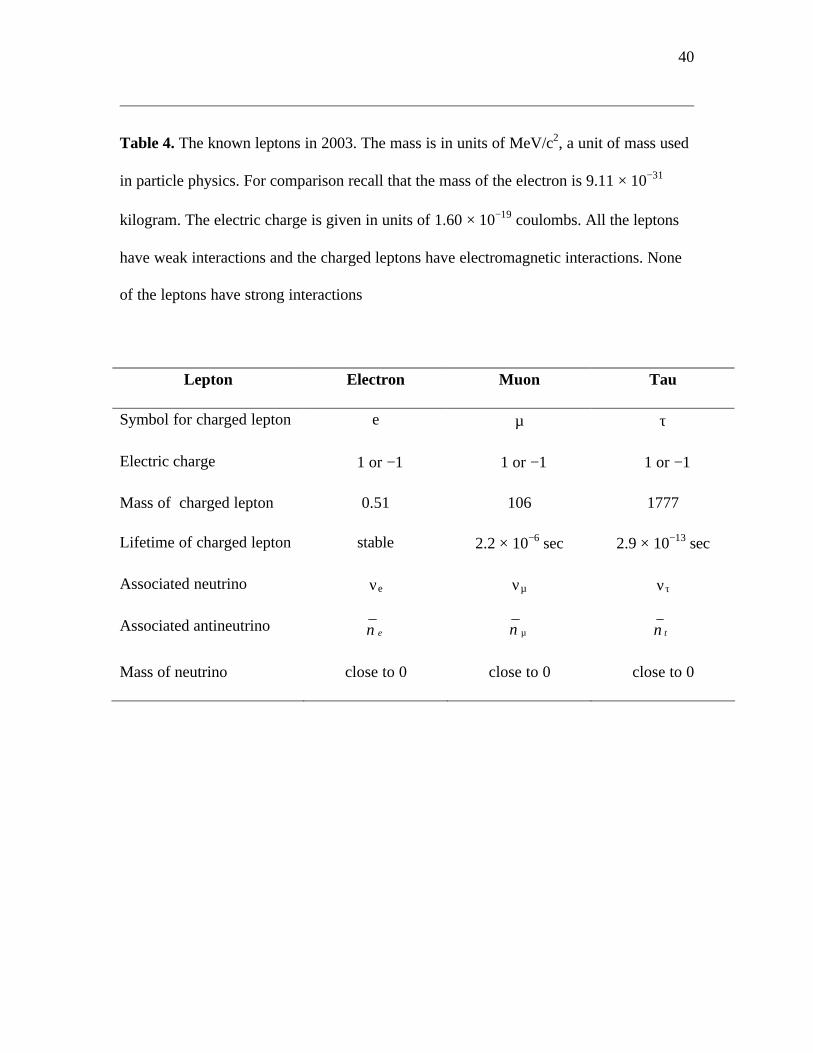
Recall that the model for the search that led to the discovery of the tau was a sequence,
possibly infinite, of increasingly massive charged leptons and a different neutrino
associated with each of the charged leptons. To my astonishment, no more charged heavy
leptons have been found in searches conducted up to about 100 GeV/c2. Also, all fully
accepted experimental results on neutrinos are satisfied by there being only three
different neutrinos associated with the e, µ, and τ. Table 4 summarizes the properties of
the three charged leptons and their neutrinos.
There is an irony in my discovery of the tau. My decision to work in lepton
physics came from the desire to understand the two 1960 puzzles associated with the
electron and the muon. The first puzzle was why the mass difference, or more generally,
what sets the masses of the elementary particles. In spite of the development of Higgs

30
theory we do not know how to specifically calculate the mass of the e or µ. In Higgs
theory we still have to put in a different parameter for each mass. The same holds for the
τ. Therefore, the discovery of the tau has added to a puzzle.
The second puzzle was: what is the intrinsic difference between the nature of the e
and the nature of the µ. Now this question has extended to the τ also. The discoveries of
the last decade that one type of neutrino can change into another type of neutrino may
lead eventually to an understanding of what constitutes the intrinsic nature of elementary
particles. But we are not there yet. Therefore the second puzzle also remains.
This is also the place to summarize my thoughts about the changes that
have occurred in elementary particle physics in the past forty years. Most
of the changes have been very good: we know a tremendous amount more
about elementary particles; we have much more powerful and sensitive
particle detectors; we have much higher energy accelerators and
colliders; and our students are better trained. But some changes, I believe,
are not so pleasant: we have lost the freedom to move quickly into new
experiments; almost all experiments are large and complicated; usually
experimenters have to work in very large collaborations; and it is no
longer possible for a particle physicist to be a productive experimenter
and at the same time be able to make calculations from first principles in
much of modern particle theory. I do not see a way to reverse these
unpleasant changes.
Acknowledgement
I am very grateful to Melodi Masaniai who worked with me on this paper, for her
substantial improvements in the presentation and format, and for her proofing and
checking of the paper.

31
This work was supported by the United States department of Energy contract DE-
AC03-76SF00515.

32
REFERENCES
1 M. L. Perl, 1996, Reflections on Experimental Science (Singapore: World Scientific,
1996).
2 M. L. Perl and M. A. Meyer, “The Practice of Experimental Physics - Recollections,
Reflections, and Interpretations,” Theoria et Historia Scientiarum: Special Issue:
Knowledge, Representation and Interpretation from Quanta to Cultures, 6 (2002) 205-
240.
3 W. Heitler, The Quantum Theory of Radiation (Oxford: Oxford University Press,
1944)
4 M. L. Perl, I. I. Rabi, and B. Senitzky, “Nuclear Electric Quadrupole Moment of Na23,”
Physical Review 97 (1955), 838-839.
5 K. W. Lai, L. W. Jones, and M. L. Perl, Proceedings of the 1960 International
Conference on Instrumentation in High-Energy Physics, Berkeley, 186-191, (1960),
edited by C. E. Mauk, A. H. Rosenfeld, and R. K. Wakerling, (New York: Interscience,
1961).
6 K. W. Lai, L. W. Jones, and M. L. Perl, “Negative Pion-Proton Elastic Scattering at
1.51, 2.01, and 2.53 Bev/c Outside the Diffraction Peak,” Physical Review Letters 7
(1961), 125-126.
7 M. L. Perl, L. W. Jones, and C. C. Ting, “Pion-Proton Elastic Scattering from 3 GeV/c
to 5 GeV/c,” Phys. Rev. 132 (1963), 1252-1272; D. E. Damouth, L. W. Jones, and M. L.
Perl, “Pion-Proton Elastic Scattering at 2.00 GeV/c,” Phys. Rev. Lett. 11 (1963), 287-290.

33
8 M. N. Kreisler, et al., “Neutron-Protron Elastic Scattering from 1 to 6 GeV,” Phys.
Rev. Lett. 16 (1966), 1217-1220.
9 M. L. Brooks, et al., (MEGA/LAMPF Collaboration), “New Limit for the Lepton-
Family-Number Nonconserving Decay µ+→e+ gamma,” Phys. Rev. Lett. 83 (1999), 1521-
1524.
10 A. Barna, et al., “Search for New Particles Produced by High-Energy Photons,” Phys.
Rev. 173 (1968), 1391-1402.
11 Y.-S. Tsai and V. Whitis, “Thick-Target Bremsstahlung and Target Considerations
for Secondary-Particle Production by Electrons,” Phys. Rev., 149 (1966), 1248-1257.
12 M. L. Perl, SLAC-PUB-1496 unpublished, (1974) 1.
13 M. L. Perl, “How Does The Muon Differ From The Electron?” Physics Today 24
(July, 1971), 34-44.
14 T. Braunstein, et al., “Comparison of Muon-Proton and Electron-Proton Scattering,”
Phys. Rev. D6 (1972), 106-136.
15 W. T. Toner, “Comparison of Muon-Proton and Electron-Proton Deep Inelastic
Scattering,” Phys. Lett. 36B (1972), 251-256.
16 R. W. Ellsworth, et al., “Muon-Proton Elastic Scattering at High Momentum
Transfers,” Phys. Rev. 165 (1968), 1449-1465; L. Camilleri, et al., “High-Energy Muon-
Proton Scattering: Muon-Electron Universality,” Phys. Rev. Lett. 23 (1969), 153-155; I.
Kostoulas, et al., “Muon-Proton Deep Elastic Scattering,” Phys. Rev. Lett. 32 (1974),
489-493.

34
17 Ya B. Zel'dovich, “Problems of Present-Day Physics and Astronomy,” Soviet Physics
Uspekhi 5 (1963), 931-950.
18 E. M. Lipmanov, “The Question of the Possible Existence of a Heavy Charged
Lepton,” Soviet Physics JETP-USSR 19 (1964), 1291-1292.
19 L. B. Okun, “On Possible Types of Elementary Particles,” Soviet Physics JETP-USSR
20, 1197-1200 (1965).
20 See for example, F. E. Low, “Heavy Electrons and Muons,” Phys. Rev. B 14, 238-239
(1965).
21 K. W. Rothe and A. M. Wolsky, “Are There Heavy Leptons,” Nucl. Phys. B 10, 241-
248 (1969).
22 G.-A. Voss, “Electron-Positron and Electron-Proton Storage Ring Colliders,”
Proceedings of the International Conference on the History of Original Ideas and Basic
Discoveries in Particle Physics, Erice, 465-485, (1996), edited by H. B. Newman and T.
Ypsilantis, (New York: Plenum Press, 1996).
23 F. T. Howard, Proceedings of the Sixth International Conference on High Energy
Accelerators, Cambridge, Mass., B43, (1967), edited by Robert A. Mack Cambridge
Electron Accelerator, Cambridge, (1967).
24 D. Ritson, et al., 1964, “Proposal for a High-Energy Electron-Positron Colliding-
Beam Storage Ring at the Stanford Linear Accelerator Center” (Stanford: SLAC, 1964).
25 N. Cabibbo and R. Gatto, “Electron-Positron Colliding Beam Experiments,” Phys.
Rev. 124 (1961), 1577-1595.
26 R. M. Larsen, et al., SLAC Proposal SP-2 (1971).
35
27 Y.-S. Tsai, “Decay Correlations of Heavy Leptons in e++e-→l++l-,” Phys. Rev. D 4,
(1971) 2821-2837.
28 H. B. Thacker and J. J. Sakurai, “Lifetimes and Branching Ratios of Heavy Leptons,”
Phys. Lett. B 36 (1971), 103-105.
29 V. Alles-Borelli, et al., “Limits on Electromagnetic Production of Heavy Leptons,”
Lettere Al Nuovo Cimento 4 (1970), 1156-1159.
30 M. Bernardi, et al., “Limits Of Mass Of Heavy Leptons,” Nuovo Cimento A 17
(1973), 383-390.
31 S. Orito, et al., “Search for Heavy Leptons with e+e- Colliding Beams,” Phys. Lett. B
48 (1974), 165-168.
32 M. L. Perl, “Anomalous Lepton Production,” Canadian Institute of Particle Physics
Summer School, McGill University, Montreal, Canada, (1975), edited by R. Heinzi and
B. Margolis, (Montreal: The Institute of Particle Physics, 1975). Page 435-488.
33 M. L. Perl, et al., “Evidence for Anomalous Lepton Production in e+-e- Annihilation,”
Phys. Rev. Lett. 35 (1975), 1489-1492.
34 M. Cavalli-Sforza, et al., “Anomalous Production of High-Energy Muons in e+e-
Collisions at 4.8 GeV,” Phys. Rev. Lett. 36 (1976), 558-561.
35 G. J. Feldman, et al., “Inclusive Anomalous Muon Production in e+e- Annihilation,”
Phys. Rev. Lett. 38 (1977), 117-120.
36 J. Burmester, et al., (PLUTO Collaboration), “Anomalous Muon Production in e+e-
Annihilation as Evidence for Heavy Leptons,” Phys. Lett. B68 (1977), 297-300.

36
37 W. Bacino, et al., “Measurement of the Threshold Behavior of the t+ t - Production in
e+ e- Annihilation,” Phys. Rev. Lett. 41 (1978), 13-15.
38 J. Kirkby, “Direct Electron Production Measurements By DELCO at SPEAR,”
Proceedings of the 1977 International Symposium on Lepton and Photon Interactions at
High Energies, Hamburg, Germany, 3-20, (1977), edited by F. Gutbrod (Hamburg:
Deutsches Elektronen-Synchrotron DESY, 1977).
39 A. Barbaro-Galtieri, et al., “Electron-Muon and Electron-Hadron Production in e+e-
Collisions,” Phys Rev Lett. 39 (1977), 1058-1061.
40 M. L. Perl, “Review of Heavy Lepton Production in e+e- Annihialtion,” Proceedings
of the 1977 International Symposium on Lepton and Photon Interactions at High
Energies, Hamburg, Germany, 145-164, (1977), edited by F. Gutbrod (Hamburg:
Deutsches Elektronen-Synchrotron DESY, 1977).
41 G. Hanson, 1978, SLAC-LBL Collaboration internal note, March 7, 1978.
42 G. J. Feldman, “e+e- Annihilation,” Proceedings of the XIX International Conference
on High-Energy Physics, Tokyo, 777-789, (1978), edited by S. Hounma and M.
Kawaguchi, (Tokyo: Physical Society of Japan, 1979).
43 R. Brandelik, et al., “Results from DASP on e+e- Annihilation between 3.1 and 5.2
GeV,” Zeitschrift Fur Physik C- Particles and Fields 1 (1979), 233-256.
44 G. S. Adams, et al., “Measurement of the Branching Fraction for tau→rho nu,” Phys.
Rev. Lett. 43 (1979), 1555-1558.

37
Tables
Table 1. The known leptons in the late 1960s. The mass is in units of MeV/c2, a unit of
mass used in particle physics. For comparison, recall that the mass of the electron is 9.11
× 10−31 kilogram. The electric charge is given in units of 1.60 × 10⁻¹⁹ coulombs.
Lepton Electron Muon
Symbol for charged lepton e µ
Electric charge +1 or −1 +1 or −1
Mass of charged lepton 0.51 106
Does particle have electromagnetic interactions? yes yes
Does particle have weak interactions? yes yes
Does particle have strong interactions? no no
Lifetime of charged lepton stable 2.2 × 10⁻⁶ sec
Associated neutrino νe νµ
Associated antineutrino ν e ν µ
Mass of neutrino close to 0 close to 0

38
Table 2. Distribution of 126 particle pair events obtained at 4.8 GeV32 with total charge
zero and no photons. In the table, e means electron, µ means muon and h means a hadron.
Type of particle pair Number found
e-e 40
e-µ 24
µ-µ 16
e-h 18
µ-h 15
h-h 13
sum 126

39
Table 3. Misidentification probabilities for the 4.8-GeV Sample32. Ph→e means the
probability that a hadron would be misidentified as an electron. Ph→µ means the
probability that a hadron would be misidentified as a muon. Ph→h means the probability
that a hadron would be identified as a hadron
Momentum range
of particle (GeV/c) Ph→e Ph→µ Ph→h
0.6–0.9 .130 ± .005 .161 ± .006 .709 ± .012
0.9–1.2 .160 ± .009 .213 ± .011 .627 ± .020
1.2–1.6 .206 ± .016 .216 ± .017 .578 ± .029
1.6–2.4 .269 ± .031 .211 ± .027 .520 ± .043
Weighted average .183 ± .007 .198 ± .007 .619 ± .012
40
Table 4. The known leptons in 2003. The mass is in units of MeV/c2, a unit of mass used
in particle physics. For comparison recall that the mass of the electron is 9.11 × 10⁻³¹
kilogram. The electric charge is given in units of 1.60 × 10⁻¹⁹ coulombs. All the leptons
have weak interactions and the charged leptons have electromagnetic interactions. None
of the leptons have strong interactions
Lepton Electron Muon Tau
Symbol for charged lepton e µ τ
Electric charge +1 or −1 +1 or −1 +1 or −1
Mass of charged lepton 0.51 106 1777
Lifetime of charged lepton stable 2.2 × 10⁻⁶ sec 2.9 × 10⁻¹³ sec
Associated neutrino νe νµ ντ
Associated antineutrino eν µν τν
Mass of neutrino close to 0 close to 0 close to 0

41
Figure Captions
Fig. 1 The principle of operation of a circular electron-positron collider. A bunch of
electrons, closed circles, and a bunch of positrons, open circles, circulate in opposite
directions in a circular ring consisting of an evacuated pipe. The cross sectional size of
the pipe is much smaller than the diameter of the ring. For example in the SPEAR
collider, figure 2, the cross sectional size of the pipe is of the order of 10 centimeters and
the diameter of the ring is about 60 meters, As the bunches circulate they pass through
each other in two places called interaction points. Almost all of the electrons and
positrons pass by each other but occasionally an electron and a positron collide and
interact producing new particles.
Fig. 2 The SPEAR electron-positron collider at the Stanford Linear Accelerator Center in
the early 1970s. The circular building with a diameter of about 80 meters contains the
collider itself. The building astride the far end of the ring with the white roof contains the
SLAC-LBL detector. Adjacent building contains the control rooms and power supplies
for the collider and the detector. Colliders are usually built underground but SPEAR was
built above ground because of budget restrictions. Courtesy Stanford Linear Accelerator
Center.

42
Fig. 3 Cross sectional view of the initial form of the SLAC-LBL detector in 1974. The
electron and positron interaction takes place at the center of the beam pipe. Particles
produced in the interaction move out from the interaction point and through the detector.
The wire chambers show the path of charge particles such as pions, electrons and muons.
The paths of these charged particles are curved because of the magnetic field produced by
the coil, the momentum of the particles is determined from the curvature. Photons from
the interaction are detected in the shower counters where they produce electromagnetic
showers. Electrons also produce electromagnetic showers in the shower counters and so
are distinguished from pions and muons. Muons produced in the interaction with
sufficient energy are detected in the muon wire chambers after they penetrate all the
layers of the detector and the 20 cm of iron.
Fig. 4 Photograph of the open SLAC-LBL detector in 1974. Some of the layers of the
detector shown schematically in Fig. 3 can be seen in this figure. Courtesy Stanford
Linear Accelerator Center.
Fig. 5 (a) The SLAC-LBL detector in 1975 with additional concrete and muon wire
chamber added on top of the detector. This addition called the muon tower enabled
cleaner detection of muons. (b) One of the first e-µ events using the tower. The µ moves
upward through the muon detector tower and the e moves downward. The numbers 13
and 113 give the relative amounts of electromagnetic shower energy deposited by the µ
and e. The six square dots show the positions of longitudinal support posts.

43
Fig. 6 The observed cross section for the signature e-µ events from the SLAC-LBL
experiment at SPEAR. This observed cross section is not corrected for acceptance. There
are 86 events with a calculated background of 22 events.33

Bunch of Positrons
Bunch of Electrons
Bunches pass through each other at interaction point
Bunches pass through each other at interaction point
X
X
Diameter of ring
Vacuum pipe
Fig. 1 The principle of operation of a circular electron-positron collider. A bunch of electrons, closed circles, and a bunch of positrons, open circles, circulate in opposite directions in a circular ring consisting of an evacuated pipe. The cross sectional size of the pipe is much smaller than the diameter of the ring. For example in the SPEAR collider, figure 2, the cross sectional size of the pipe is of the order of 10 centimeters and the diameter of the ring is about 60 meters, As the bunches circulate they pass through each other in two places called interaction points. Almost all of the electrons and positrons pass by each other but occasionally an electron and a positron collide and interact producing new particles.

Fig. 2 The SPEAR electron-positron collider at the Stanford Linear Accelerator Center in the early 1970s. The circular building with a diameter of about 80 meters contains the collider itself. The building astride the far end of the ring with the white roof contains the SLAC-LBL detector. Adjacent building contains the control rooms and power supplies for the collider and the detector. Colliders are usually built underground but SPEAR was built above ground because of budget restrictions.

Trigger Counters (4)
Cylindrical Wire Chambers
Muon Wire Chambers
Shower Counters (24)Iron (20 cm)
CoilTrigger Counters (48)
B
Beam Pipe
Proportional Chambers (2)Support
Post (6)
1 meter
x
Fig. 3. Cross sectional view of the initial form of the SLAC-LBL detector in 1974. The electron and positron interaction takes place at the center of the beam pipe. Particles produced in the interaction move out from the interaction point and through the detector. The wire chambers show the path of charge particles such as pions, electrons, and muons. The paths of these charged particles are curved because of the magnetic field produced by the coil, the momentum of the particles is determined from the curvature. Photons from the interaction are detected in the shower counters where they produce electromagnetic showers. Electrons also produce electromagnetic showers in the shower counters and so are distinguished from pions and muons. Muons produced in the interaction with sufficient energy are detected in the muon wire chambers after they penetrate all the layers of the detector and the 20 cm of iron.

Fig. 4 Photograph of the open SLAC-LBL detector in 1974. Some of the layers of the detector shown schematically in Fig. 3 can be seen in this figure.

Proportional Chambers
Pipe Counter
Coil
Coil
Muon Spark Chambers
Shower Counters
Trigger Counters
Luminosity Monitor
Compensating Solenoid
Muon Absorber
Muon Absorber
Flux Return
Beam PipeEndÐCap Chambers
Wire Spark Chambers
x
13
113
x
x
x
x
x
x x
xx
xxx
x
(b)
(a)
Fig. 5(a). The SLAC-LBL detector in 1975 with additional concrete and muon wire chamber added on top of the detector. This addition called the muon tower enabled cleaner detection of muons. (b) One of the first e-µ events using the tower. The µ moves upward through the muon detector tower and the e moves downward. The numbers 13 and 113 give the relative amounts of electromagnetic shower energy deposited by the µ and e. The six square dots show the positions of longitudinal support posts.
2 4 6 80
10
20
30
σ eµ,
obs
erve
d (
10—
36 c
m2 )
Total Energy (GeV) 9—927243A25
Fig. 6 The observed cross section for the signature e-µ events from the SLAC-LBL experiment at SPEAR. This observed cross section is not corrected for acceptance. There are 86 events with a calculated background of 22 events.33