SLAGGING IN ENTRAINED-FLOW GASIFIERS · th gasifier, five gasification tests were completed with the characterized coals. Solid samples from the refractory liners, in-situ gas sampling

$Page 1: SLAGGING IN ENTRAINED-FLOW GASIFIERS · th gasifier, five gasification tests were completed with the characterized coals. Solid samples from the refractory liners, in-situ gas sampling$
SLAGGING IN ENTRAINED-FLOW

GASIFIERS

Marc A. Duchesne

Thesis submitted to the

Faculty of Graduate and Postdoctoral Studies

In partial fulfillment of the requirements

For the PhD degree in Chemical Engineering

Department of Chemical and Biological Engineering

Faculty of Engineering University of Ottawa

© Marc Duchesne, Ottawa, Canada, 2012

ii

Statement of Contribution of Collaborators

Chapters 3-8 of this thesis take the form of research papers which include work from

collaborators, as detailed below. I am the sole author of all other chapters. My

supervisors, Dr. Arturo Macchi of the Department of Chemical and Biological

Engineering, University of Ottawa, and Dr. Edward John Anthony of CanmetENERGY,

Natural Resources Canada, supervised my work during the Ph.D. program and provided

editorial corrections.

For Chapter 3, I authored the paper. The modeling concept is mine. I developed the

artificial neural network model, compared it to other models and applied it to case

studies.

For Chapter 4, I authored 80% of the paper. The toolbox concept is mine. I developed

80% of the toolbox. Mr. Bronsch and Dr. Masset authored 20% of the paper and

developed 20% of the toolbox.

For Chapter 5, I authored the paper. I assembled the CanmetENERGY slag viscosity

measurement system with help from Dr. Hughes, Mr. McCalden and Dr. Lu. Dr.

Ilyushechkin and I performed the viscosity measurements and slag quenching

experiments. Dr. Ilyushechkin completed the electron microscopy analysis. I completed

the FactSage modeling. Dr. Ilyushechkin and I analysed all the results.

For Chapter 6, Dr. Ilyushechkin authored the paper. Dr. Ilyushechkin performed the

quenching experiments and completed the electron microscopy analysis. Dr. Ilyushechkin

and I performed the viscosity measurements. Dr. Ilyushechkin and I analysed all the

results.

iii

For Chapter 7, I authored the paper. I performed or supervised the viscosity

measurements. I completed the cup tests and FactSage modeling. I developed the

characterization program and analysed all the results.

For Chapter 8, with the exception of the gasifier system description which was written by

Dr. Hughes, I authored the paper. Dr. Hughes, Mr. McCalden and Dr. Lu are responsible

for the design and operation of the gasifier system. I assisted in the gasifier maintenance

and sample collection. Dr. Hughes and I developed the pilot testing program. Dr. Lu and

I preformed the surface area and density measurements. I performed the surface

roughness measurements. I developed the solid sample analysis program and analysed all

the results.

Signature: _____________________ Date: _________________

iv

Abstract

Gasification is a flexible technology which is applied in industry for electricity

generation, hydrogen production, steam raising and liquid fuels production. Furthermore,

it can utilize one or more feedstocks such as coal, biomass, municipal waste and

petroleum coke. This versatility, in addition to being adaptable to various emissions

control technologies (including carbon capture) renders it an attractive option for years to

come. One of the most common gasifier types is the entrained-flow slagging gasifier. The

behaviour of inorganic fuel components in these gasifiers is still ill-understood even

though it can be the determining factor in their design and operation. A literature review

of inorganic matter transformation sub-models for entrained-flow slagging gasifiers is

provided. Slag viscosity was identified as a critical property in the sub-models.

Slag viscosity models are only applicable to a limited range of slag compositions and

conditions, and their performance is not easily assessed. An artificial neural network

model was developed to predict slag viscosity over a broad range of temperatures and

slag compositions. This model outperforms other slag viscosity models, resulting in an

average absolute logarithmic error of 0.703 when applied to validation data. Furthermore,

a toolbox was developed to assist slag viscosity model users in the selection of the best

model for given slag compositions and conditions, and to help users determine how well

the best model will perform. The toolbox includes a slag viscosity prediction calculator

with 24 slag viscosity models, and a database of 4124 slag viscosity measurements.

Petroleum coke may be used as a fuel for entrained-flow slagging gasification. The slag

viscosities of coal, petroleum coke and coal/petroleum coke blends were measured in the

temperature range of 1175-1650ºC. Two different viscosity measurement apparatuses

were used in separate laboratories. Some viscosity measurements were repeated to test

reproducibility of the results. Some effects of blending on viscosity can be explained by

network former and modifier theory. Other effects are attributed to solids formation

which was investigated via slag quenching experiments and phase equilibrium

v

predictions. Below 1300°C, vanadium, a major component of petroleum coke ashes,

promotes the formation of spinel which increases slag viscosity. Unfortunately, slags

containing vanadium species react readily with the crucible and spindle materials used for

viscosity measurements. Interaction of vanadium-rich slags with various materials was

investigated. The bulk and phase compositions of two petroleum coke slags on Al2O3,

Mo, Pt and Ni supports were analysed, and kinetics of slag compositional changes at

1400 °C were determined. Mechanisms of the slag interactions with supports are

described. Viscosity of slags with Mo, Ni and Al2O3 supports are compared in the

temperature range 1200-1500 °C.

The results from the first two parts of a three-part research program which involves fuel

characterization, testing in a 1 MWth gasifier, and computational fluid dynamics (CFD)

modeling for entrained-flow slagging gasification are presented. The end goal is to

develop a CFD model which includes inorganic matter transformations. Initially, four

coals were selected for this program and one limestone was chosen as a fluxing agent.

Fuel properties were determined with prioritization based on their application; screening

of potential fuels, ensuring proper gasifier operation, gasifier design and/or CFD

modeling. Of the four coals tested, one was deemed unsuitable based on initial screening

tests. Two of the three remaining coals require fluxing for proper gasifier operation.

Using CanmetENERGY’s 1 MWth gasifier, five gasification tests were completed with

the characterized coals. Solid samples from the refractory liners, in-situ gas sampling

probe sheaths and impingers, the slag tap, the slag pot, quench discharge water and

scrubber water were collected and characterized. Char and fly ash samples indicate that

most of the inorganic matter melted and formed spheres. Devolatilization and interaction

with the gasifier refractory affected the composition of slag collected from the gasifier.

Signs of refractory spalling/erosion were detected. The slag layers formed on the alumina

liners are smooth with some rivulets and spotting. The slag layers formed on the alumina-

chromia liners are rough and bubbly. Slag penetration fractions were determined for all

liners.

vi

Sommaire

La gazéification est une technologie flexible qui est appliquée en industrie pour la

génération d'électricité, la production d'hydrogène, la formation de vapeur et la

production de carburants liquides. En outre, elle peut consommer un ou plusieurs types

de carburants comme le charbon, la biomasse, les déchets municipaux et le coke de

pétrole. Cette polyvalence, en plus d'être adaptable à différentes technologies pour

contrôler les émissions (y compris le dioxyde de carbone) rend la gazéification une

option attrayante pour les années à venir. L'un des types les plus courants de gazéificateur

est le gazéificateur à flux entraîné. Le comportement de matières inorganiques dans ces

gazéificateurs est encore mal compris, malgré le fait que ça peut être le facteur

déterminant dans la conception et le fonctionnement des gazéificateurs. Une revue de la

littérature sur les sous-modèles pour les transformations de la matière inorganique dans

les gazéificateurs à flux entraîné est fournie. La viscosité du mâchefer a été identifiée

comme une propriété essentielle pour les sous-modèles.

Les modèles de viscosité pour le mâchefer ne sont applicables qu'à des compositions et

conditions limitées. De plus, leur performance n'est pas facile à évaluer. Un modèle à

réseau neuronal artificiel, applicable à une large plage de températures et compositions, a

été développé pour prédire la viscosité du mâchefer. Ce modèle surpasse autres modèles

de viscosité, résultant en une erreur logarithmique absolue moyenne de 0,703 lorsqu'il est

appliqué à des données de validation. De plus, une boîte à outils a été conçue pour

assister les utilisateurs de modèles de viscosité du mâchefer. La boîte d’outils permet la

sélection du meilleur modèle pour des compositions et conditions d’intérêts par

prédiction de la performance de divers modèles. La boîte à outils comprend un

calculateur de prédictions avec 24 modèles, et une base de données avec 4124 mesures.

Le coke de pétrole peut être utilisé comme carburant pour la gazéification à flux entraîné.

La viscosité de mâchefers provenant de charbon, coke de pétrole, et mélanges de charbon

et coke de pétrole a été mesurée dans la gamme de température de 1175-1650 °C. Deux

vii

différents appareils de mesure de viscosité ont été utilisés dans des laboratoires

indépendants. Certaines mesures de viscosité ont été répétées pour vérifier la

reproductibilité des résultats. Certains effets sur la viscosité du mâchefer résultant de

l’ajout du coke de pétrole au charbon peuvent être expliqués par la théorie de formeurs et

modificateurs de réseaux dans les fondus de silices. D'autres effets sont attribués à la

formation de matières solides qui a été étudiée par l’analyse de mâchefers refroidis, ainsi

que par prédictions d'équilibre de phases. En dessous de 1300 °C, le vanadium, un

composant majeur des cendres du coke de pétrole, favorise la formation de spinelle qui

augmente la viscosité du mâchefer. Malheureusement, les mâchefers contenant du

vanadium réagissent aisément avec les matériaux de creuset utilisés pour la mesure de

viscosité. Les interactions de divers matériaux avec mâchefers riches en vanadium ont été

étudiées. Les compositions moyennes et de phases de deux mâchefers provenant de cokes

de pétrole placés sur du Al2O3, Mo, Pt ou Ni ont été analysées. La cinétique des

changements de compositions pour les mâchefers à 1400 °C a été déterminée. Les

mécanismes d’interactions avec les matériaux sont décrits. Une comparaison de la

viscosité du mâchefer mesurée à l’aide de creusets en Mo, Ni et Al2O3 est effectuée dans

l'intervalle de température de 1200 à 1500 °C.

Les résultats des deux premiers volets d'un programme de recherche qui comprend la

caractérisation de carburants, des essais avec un gazéificateur de 1 MWth, et la mécanique

des fluides numérique (MFN) pour la gazéification à flux entraîné sont présentés.

L'objectif final est de développer un modèle MFN de gazéification qui prend compte des

transformations de la matière inorganique. Initialement, quatre charbons ont été choisis

pour ce programme et un calcaire a été choisi comme agent fluxant. Les propriétés des

carburants ont été déterminées avec une hiérarchisation en fonction de leur application; le

dépistage des carburants potentiels, assurer un bon fonctionnement du gazéificateur, la

conception du gazéificateur, et/ou la modélisation MFN. Parmi les quatre charbons

choisis, l'un a été éliminé en tant que carburant potentiel. Deux des trois charbons restants

nécessitent un agent fluxant pour le bon écoulement du mâchefer. En utilisant le

gazéificateur de 1 MWth à CanmetÉNERGIE, cinq essais de gazéification ont été réalisés

avec les charbons caractérisés. Des échantillons provenant de doublures réfractaires,

viii

gaines et filtres à la sonde de gaz in-situ, l’embouchure du mâchefer, le pot de mâchefer,

l'eau de décharge et l’absorbeur ont été recueillis et caractérisés. L’analyse de cendres

volantes indique que la plupart de la matière inorganique est fondue et en forme de

sphères. La dévolatilisation et l'interaction avec le réfractaire ont modifié la composition

du mâchefer. L'effritement du réfractaire a été observé. Le mâchefer sur les doublures

d'alumine est discontinu et forme des taches circulaires. Le mâchefer sur les doublures

d'alumine-chrome est rugueux et bulleux. La fraction de pénétration par le mâchefer dans

les doublures réfractaires a été déterminée.

ix

Acknowledgements

First and foremost, I wish to thank my co-supervisors Arturo Macchi and E. J. ‘Ben’

Anthony for believing in my capabilities, providing guidance and opening doors to

possibilities far beyond what I could have dreamed.

I wish to also thank my colleagues at CanmetENERGY for sharing their passion and

dedication. Robin Hughes, David McCalden and Dennis Lu were integral to the progress

of my research. Special thanks go to Jeffery Slater, Ryan Burchat, Robert Symonds, Firas

Ridha, Vasilije Manovic, members of the Characterization Laboratory, Alan

Vaillancourt, Richard Lacelle, and many more at the CanmetENERGY Bells Corners

complex.

In the process of completing work for this thesis, I have made many friends abroad. They

have provided different perspectives which improved the quality of my work and my life

in general. The gasification research group at CSIRO and the Vithucon Multiphase

Sytsems group at the TU Bergakademie Freiberg were gracious hosts for extended

periods of time.

I am indebted to my family and friends for their care and encouragement. Listening to my

sister’s advice and trying to copy her strong qualities have proved fruitful time and again.

I cannot thank enough my parents who continue to support me in all my endeavors. My

friends have kept me sane and answered the call when I needed them most. My beloved

Elysa provided the greatest motivation of all.

Lastly, I wish to acknowledge financial assistance from the Natural Sciences and

Engineering Research Council of Canada, Natural Resources Canada, and the University

of Ottawa.

x

Table of Contents

STATEMENT OF CONTRIBUTION OF COLLABORATORS......................................................... II

ABSTRACT.......................................................................................................................................... IV

SOMMAIRE.........................................................................................................................................VI

ACKNOWLEDGEMENTS.................................................................................................................. IX

TABLE OF CONTENTS....................................................................................................................... X

LIST OF TABLES............................................................................................................................. XIV

LIST OF FIGURES........................................................................................................................... XVI

CHAPTER 1. INTRODUCTION..................................................................................................... 1

1.1 MOTIVATION TO DEVELOP GASIFICATION .................................................................................. 1 1.2 FUELS OF INTEREST .................................................................................................................. 2 1.3 GASIFICATION BASICS............................................................................................................... 4 1.4 RESEARCH OBJECTIVES AND OUTLINE........................................................................................ 8 1.5 REFERENCES ............................................................................................................................ 9

CHAPTER 2. LITERATURE REVIEW OF INORGANIC MATTER TRANSFORMATION

SUB-MODELS FOR ENTRAINED-FLOW SLAGGING GASIFIERS ............................................. 12

2.1 INTRODUCTION....................................................................................................................... 12 2.2 ASH PARTICLE FORMATION ..................................................................................................... 13

2.2.1 Chemical fractionation and CCSEM .............................................................................. 14 2.2.2 Ash formation................................................................................................................ 16

2.3 GAS-PARTICLE TRANSPORT ..................................................................................................... 20 2.4 PARTICLE STICKING ................................................................................................................ 22 2.5 SLAG FLOW ............................................................................................................................ 27 2.6 SLAG-REFRACTORY INTERACTIONS ......................................................................................... 33 2.7 REFERENCES .......................................................................................................................... 36

CHAPTER 3. ARTIFICIAL NEURAL NETWORK MODEL TO PREDICT SLAG VISCOSITY

OVER A BROAD RANGE OF TEMPERATURES AND SLAG COMPOSITIONS......................... 42

3.1 ABSTRACT ............................................................................................................................. 43 3.2 INTRODUCTION....................................................................................................................... 44 3.3 SLAG VISCOSITY ..................................................................................................................... 45

3.3.1 Parameters affecting viscosity........................................................................................ 45 3.3.2 Previous models ............................................................................................................ 46

xi

3.4 ARTIFICIAL NEURAL NETWORK MODELING OF SLAG VISCOSITY................................................. 49 3.4.1 Dataset and input variable selection .............................................................................. 49 3.4.2 Performance function .................................................................................................... 51 3.4.3 Architecture and training............................................................................................... 52 3.4.4 Comparison of models ................................................................................................... 53

3.5 GENESEE COAL ASH VISCOSITY PREDICTIONS WITH VARYING AMOUNTS OF FLUXING AGENTS .... 55 3.6 CONCLUSION .......................................................................................................................... 60 3.7 ACKNOWLEDGEMENTS ........................................................................................................... 61 3.8 REFERENCES .......................................................................................................................... 61

CHAPTER 4. SLAG VISCOSITY MODELING TOOLBOX....................................................... 64

4.1 ABSTRACT ............................................................................................................................. 65 4.2 ACRONYMS ............................................................................................................................ 66 4.3 INTRODUCTION....................................................................................................................... 66 4.4 CALCULATION ........................................................................................................................ 67

4.4.1 Slag viscosity predictor tool........................................................................................... 67 4.4.2 Slag viscosity database tool ........................................................................................... 68 4.4.3 Artificial neural network model for fully molten slags..................................................... 69 4.4.4 Application of the Roscoe-Einstein model for partially crystallized slags ........................ 72

4.5 RESULTS AND DISCUSSION ...................................................................................................... 73 4.5.1 Case Study 1 – Glass formation ..................................................................................... 78 4.5.2 Case Study 2 – Entrained flow gasification .................................................................... 79 4.5.3 Case Study 3 – Blast furnace.......................................................................................... 80

4.6 CONCLUSION .......................................................................................................................... 81 4.7 ACKNOWLEDGEMENTS ........................................................................................................... 81 4.8 REFERENCES .......................................................................................................................... 82

CHAPTER 5. FLOW BEHAVIOUR OF SLAGS FROM COAL AND PETROLEUM COKE

BLENDS 85

5.1 ABSTRACT ............................................................................................................................. 86 5.2 INTRODUCTION....................................................................................................................... 87 5.3 EXPERIMENTAL ...................................................................................................................... 89

5.3.1 Coal and petroleum coke selection................................................................................. 89 5.3.2 Viscosity measurements ................................................................................................. 90 5.3.3 Quenching experiments.................................................................................................. 92 5.3.4 Sample analysis ............................................................................................................. 92 5.3.5 FactSage predictions ..................................................................................................... 92

5.4 RESULTS ................................................................................................................................ 93

xii

5.4.1 Validation of viscosity measurements............................................................................. 93 5.4.2 Viscosity of blends ......................................................................................................... 94 5.4.3 Slag microstructure ....................................................................................................... 98 5.4.4 Reactivity with crucible and spindle ............................................................................. 103

5.5 DISCUSSION ......................................................................................................................... 104 5.6 CONCLUSION ........................................................................................................................ 106 5.7 ACKNOWLEDGEMENTS ......................................................................................................... 107 5.8 REFERENCES ........................................................................................................................ 107

CHAPTER 6. INTERACTIONS OF VANADIUM-RICH SLAGS WITH CRUCIBLE

MATERIALS DURING VISCOSITY MEASUREMENTS .............................................................. 109

6.1 ABSTRACT ........................................................................................................................... 110 6.2 INTRODUCTION..................................................................................................................... 111 6.3 EXPERIMENTAL .................................................................................................................... 112

6.3.1 Sample preparation ..................................................................................................... 112 6.3.2 Sample analysis ........................................................................................................... 114 6.3.3 Viscosity measurements ............................................................................................... 115

6.4 RESULTS AND DISCUSSION .................................................................................................... 115 6.4.1 Slag processed in Al2O3 ............................................................................................... 115 6.4.2 Slag processed in Mo................................................................................................... 120 6.4.3 Slag processed in Pt or Ni............................................................................................ 126 6.4.4 Mechanisms of slag-support interactions ..................................................................... 130 6.4.5 Bulk compositional changes and viscosity .................................................................... 132 6.4.6 Application of the results to viscosity measurements..................................................... 135

6.5 CONCLUSION ........................................................................................................................ 139 6.6 REFERENCES ........................................................................................................................ 140

CHAPTER 7. FATE OF INORGANIC MATTER IN ENTRAINED-FLOW SLAGGING

GASIFIERS: FUEL CHARACTERIZATION.................................................................................. 143


7.3.1 FactSage modeling ...................................................................................................... 148 7.3.2 Slag viscosity measurements ........................................................................................ 148 7.3.3 Cup tests for slag-refractory reactivity ......................................................................... 149 7.3.4 Coal petrography to determine fuel form...................................................................... 150 7.3.5 CCSEM....................................................................................................................... 150 7.3.6 Other methods ............................................................................................................. 151

xiii

7.4 RESULTS AND DISCUSSION .................................................................................................... 152 7.4.1 Screening .................................................................................................................... 152 7.4.2 Operation.................................................................................................................... 157 7.4.3 Design......................................................................................................................... 160 7.4.4 CFD modeling............................................................................................................. 169

7.5 CONCLUSIONS ...................................................................................................................... 172 7.6 ACKNOWLEDGEMENTS ......................................................................................................... 173 7.7 REFERENCES ........................................................................................................................ 173

CHAPTER 8. FATE OF INORGANIC MATTER IN ENTRAINED-FLOW SLAGGING

GASIFIERS: PILOT PLANT TESTING .......................................................................................... 179


8.3.1 Gasifier system............................................................................................................ 183 8.3.2 Surface roughness measurements................................................................................. 187 8.3.3 Surface area and density.............................................................................................. 188 8.3.4 Other methods ............................................................................................................. 189

8.4 RESULTS AND DISCUSSION .................................................................................................... 190 8.4.1 Description of pilot plant tests ..................................................................................... 190 8.4.2 Char and fly ash .......................................................................................................... 193 8.4.3 Slag from the slag tap, slag pot and quench water discharge ........................................ 201 8.4.4 Slag layer on refractory ............................................................................................... 204 8.4.5 Slag-refractory interface.............................................................................................. 211

8.5 CONCLUSION ........................................................................................................................ 214 8.6 ACKNOWLEDGEMENTS ......................................................................................................... 215 8.7 REFERENCES ........................................................................................................................ 215

CHAPTER 9. CONCLUSIONS AND RECOMMENDATIONS................................................. 218

9.1 SLAG VISCOSITY MEASUREMENTS ......................................................................................... 218 9.2 SLAG VISCOSITY MODELING .................................................................................................. 221 9.3 MODELING TRANSFORMATIONS OF INORGANIC MATTER IN ENTRAINED-FLOW SLAGGING

GASIFIERS......................................................................................................................................... 225 9.4 REFERENCES ........................................................................................................................ 227

APPENDIX A ..................................................................................................................................... 232

xiv

List of Tables Table 1.1: Properties of coals...........................................................................................2

Table 1.2: Properties of petroleum cokes .........................................................................3

Table 1.3: Coal ash major and minor oxides expressed as wt.%.......................................3

Table 1.4: Petroleum coke ash major and minor oxides expressed as wt.% ......................4

Table 1.2: Viscosity of common fluids ............................................................................7

Table 3.1: Datasets used for ANN models in this study..................................................50

Table 3.2: Input and output ranges of ANN models in this study ...................................51

Table 3.3: Average absolute logarithmic errors of compared models for each dataset

group.............................................................................................................................54

Table 3.4: ANN1 weight values.....................................................................................55

Table 3.5: Genesee coal ash composition.......................................................................57

Table 3.6: Compositions of fluxing agents.....................................................................57

Table 4.1: Weight values for ANNliq ............................................................................71

Table 4.2: Average absolute logarithmic error (AALE) of slag viscosity models applied

to data used for the development of the ANNliq model..................................................72

Table 4.3: Average absolute logarithmic error (AALE) of slag viscosity models with and

without the Roscoe-Einstein (RE) modification .............................................................73

Table 4.4: Selection criteria for each case study.............................................................75

Table 4.5: Number of measurements identified and average absolute logarithmic error

(AALE) of slag viscosity models for each case study.....................................................77

Table 5.1: Composition of coal and petcoke ashes/slags ................................................89

Table 5.2: Composition of vanadium-rich slags before and after viscosity tests ........... 104

Table 6.1: Composition of petcoke ashes (wt.%) and crucibles used in the study ......... 113

Table 6.2: Phase compositions (wt.%) of P1and P2 slags with Al2O3 crucibles ............ 117

xv

Table 6.3: Phase compositions (wt.%) of P1and P2 slags with Mo crucibles................ 122

Table 6.4: Phase compositions (wt.%) of P1 slags with Pt crucibles............................ 127

Table 6.5: Phase compositions (wt.%) of P1 slags with Ni crucibles ............................ 129

Table 6.6: Composition of V-rich slags before (P1 and P2) and after viscosity tests.....133

Table 7.1: Fuel properties involved in inorganic matter phenomena............................. 147

Table 7.2: Proximate analysis, ultimate analysis and gross calorific value ................... 153

Table 7.3: Inorganic matter composition...................................................................... 154

Table 7.4: Ash fusion temperatures in °C..................................................................... 156

Table 7.5: Diffusion predictions .................................................................................. 163

Table 7.6: Normalized atomic compositions of slags reacted with refractories ............. 166

Table 7.7: Normalized atomic compositions of refractories reacted with slag .............. 167

Table 8.1: Conditions for pilot-scale gasifier tests........................................................ 191

Table 8.2: Ash content, carbon content and mass of dried collected solids ................... 192

Table 8.3: Ash mass balance........................................................................................ 193

Table 8.4: Carbon mass balance .................................................................................. 193

Table 8.5: Major and minor oxides in ash of collected solid samples ........................... 194

Table 8.6: Quantitative XRD analyses for solid samples .............................................. 196

Table 8.7: Surface area, skeletal density, envelope density and porosity of solid samples

....................................................................................................................................198

Table 8.8: Ash injection rates and slag layer properties................................................ 206

xvi

List of Figures Figure 1.1: Schematic diagram of top-fired entrained-flow slagging gasifier....................5

Figure 2.1: Schematic diagram of slag deposited on a gasifier wall. ...............................28

Figure 3.1: Viscosity predictions for Genesee coal ash with varying amounts of FA1…..

......................................................................................................................................58


......................................................................................................................................59


......................................................................................................................................60

Figure 5.1: Temperature-LV curves demonstrating repeatability and reproducibility of

slag viscosity measurements, with and without sulphur, at CanmetENERGY (labeled CE)

and CSIRO (labeled CSIRO). ........................................................................................94

Figure 5.2: Temperature-LV curves of coal and petcoke slag blends. Dashed lines are

drawn at 25 Pa·s. ...........................................................................................................96

Figure 5.3: Microstructure of slags quenched from 1350 °C: C1b (a), C1b+50P1b (b),

C1b+100P1b (c); and quenched from 1300 °C: C1b (d), C1b+50P1b (e), C1b+100P1b

(f). Legend: Liq- former liquid phase, Mul- mullite, Spi- spinel. ....................................99

Figure 5.4: Microstructure of slags quenched from 1200 °C: S1 (a), S1+25P1a (b),

S1+50P1a (c). Legend: Liq- former liquid phase, Fel- feldspar, Spi- spinel....................99

Figure 5.5: Microstructure of slags quenched from 1250 °C: S2 (a), S2+50P1 (b),

S2+2.2V2O5 (c). Legend: Liq- former liquid phase, Fel- feldspar, Mul- mullite, Spi-

spinel.............................................................................................................................99

Figure 5.6: Microstructure of slags quenched from 1325 °C: S3 (a), S4 (b), S3+5V2O5

(c); and quenched from 1275 °C: S3 (d), S4 (e), S3+5V2O5 (f). Legend: Liq- former

liquid phase, Fel- feldspar, Spi- spinel. ........................................................................ 100

Figure 5.7: Predicted solids mass fractions of coal and petcoke slag blends using

FactSage...................................................................................................................... 101

xvii

Figure 5.8: Microstructure of slags in Mo (a) and alumina (b) crucibles....................... 103

Figure 6.1: Temperature profiles used for slag preparation and processing................... 114

Figure 6.2: Microstructures of slow cooled P1 (a) and P2 (b) slags with Al2O3 supports

after processing with Profile 1.. ................................................................................... 116

Figure 6.3: Microstructures of P1 and P2 slags on Al2O3 supports quenched from 1400

°C: P1 after 1h (a), P1 after 12 h (b), P2 after 1h (c), and P2 after 12h (d).................... 118

Figure 6.4: V2O3 and Al2O3 content in P1 (a, b) and in P2 (c, d) slags on Al2O3 supports

quenched from 1400 °C. ............................................................................................. 119

Figure 6.5: Microstructures of slow cooled slags P1 (a) and P2 (b) on Mo supports after

processing with Profile 1.. ........................................................................................... 121

Figure 6.6: Microstructures of P1 and P2 slags on Mo supports quenched from 1400 °C:

P1 after 1h (a), P1 after 12 h (b), P2 after 1h (c), and P2 after 12h (d).......................... 124

Figure 6.7: Solid phase content in P1 and P2 slags on Mo supports quenched from 1400

°C................................................................................................................................ 124

Figure 6.8: V2O3 and MoO3 content in P1 (a, b) and in P2 (c, d) slags on Mo supports

quenched from 1400 °C. .............................................................................................. 125

Figure 6.9: Microstructures of P1 slags equilibrated with Pt supports at 1400 °C for 1 h

(a) and 12 h (b)............................................................................................................ 127

Figure 6.10: Microstructures of P1 slags processed with Ni. Slag was quenched after 0.5

h (a) and 1.5 h (b) at 1320 °C. Slag was also quenched from 1390 °C during Profile 1 (c)

and slowly cooled after Profile 1 (d).. .......................................................................... 129

Figure 6.11: Mechanisms of slag interaction with Al2O3 supports................................ 131

Figure 6.12: Mechanisms of slag interaction with Mo supports....................................132

Figure 6.13: Viscosity versus temperature for P1 (a) and P2 (b) slags processed with

different support materials. .......................................................................................... 134

Figure 7.1: Solids mass fractions predicted using FactSage.......................................... 156

Figure 7.2: Measured slag viscosities........................................................................... 159

xviii

Figure 7.3: Silicon (Si), aluminum (Al) and iron (Fe) elemental maps produced by SEM-

EDX of F1 on alumina at 1250°C (a), alumina at 1500°C (b), silicon carbide at 1250°C

(c), silicon carbide at 1500°C (d), alumina-chromia at 1250°C (e) and alumina-chromia at

1500°C (f). The scale in the left (a) image applies to all images. ..................................164

Figure 8.1: Schematic diagram of CanmetENERGY’s pressurized entrained-flow

gasification system. ..................................................................................................... 184

Figure 8.2: Schematic diagram of the gas probe inserted into the gasifier. ................... 186

Figure 8.3: Surface roughness measurement system..................................................... 188

Figure 8.4: SEM images comparing scrubber and probe impinger samples: (a) T1

scrubber, (b) T2 scrubber, (c) T4 scrubber, (d) T5 scrubber, (e) T1 impinger, (f) T3

impinger and (g) T4 impinger.. .................................................................................... 199

Figure 8.5: Slag collected from the slag pot after test T5 (a) and classified according to

shape: (b) slag chunks, (c) slag filaments and (d) slag sheets. ...................................... 203

Figure 8.6: Photos of liners (a-e) from tests T1-T5, respectively. .................................207

Figure 8.7: Roughness of slag surface on liners. .......................................................... 208

Figure 8.8: Photos of probe sheaths (a-e) from tests T1-T5, respectively. .................... 210

Figure 8.8: Silicon (Si), aluminum (Al) and calcium (Ca) elemental maps produced by

SEM-EDX of slag-refractory cross-sections for tests T1 (a) and T2 (b).. ..................... 212

Figure 8.9: Slag penetration in alumina-chromia refractory. ........................................ 213

Figure A.1: First generation molybdenum spindle specifications. ................................ 233

Figure A.2: First generation molybdenum crucible specifications. ............................... 233

Figure A.3: Second generation molybdenum spindle specifications. ............................ 234

Figure A.4: Second generation molybdenum crucible specifications. ........................... 234

Figure A.5: Alumina spindle specifications. ................................................................ 235

Figure A.6: Alumina crucible specifications.. .............................................................. 236

Figure A.7: First generation base specifications. . ........................................................ 237

xix

Figure A.8: First generation cap specifications.. .......................................................... 238

Figure A.9: Second generation base specifications. ..................................................... 239

Figure A.10: Second generation cap specifications.. .................................................... 240

1

Chapter 1. INTRODUCTION

1.1 Motivation to develop gasification

Worldwide, coal is used for roughly 39% of all electricity generation and 24% of total

energy usage [1]. Not only is coal cheap, but it is also plentiful [2]. There however are

many downsides to coal consumption. For example, conventional coal burning produces

considerably more carbon dioxide per unit of electricity when compared to burning oil or

natural gas [3]. One of the reasons for this is the low efficiency of coal energy

conversion. Standard plants burn coal in a boiler to produce heat. This heat is used to

produce steam which will turn a steam turbine. The mechanical energy from the turbine

is then converted to electricity. Integrated gasification combined cycles (IGCCs) provide

an alternative to generate electricity from coal. They allow for thorough gas clean-up and

the technology is a front-runner for carbon capture and sequestration projects. From a

Canadian perspective, front-end engineering and design (FEED) work was conducted on

a 270 MW coal-fired IGCC that may be constructed in Alberta [4]. Capital Power

announced in October 2009 that it would not move forward with construction of this

plant at present due to the drop in electricity price, although the FEED will be completed

and could serve as a blueprint for a future project. Alternatively, gasification may prosper

in Alberta due to a suggested scheme which integrates petroleum coke gasification with

carbon capture and storage to yield hydrogen, power, and steam production for oil sands

upgrading with near zero CO2 emissions. Notwithstanding, smaller scale gasification

projects are already operating across Canada. Around the world, many gasification plants,

including IGCCs, have been running for decades and new ones are continually being

added to the commercial pipeline [5].

2

1.2 Fuels of interest

The fuels considered in this thesis are coals and petroleum cokes due to their potential for

large-scale gasification in Canada. Coals are generally classified as anthracite,

bituminous, subbituminous or lignite. Table 1.1 provides typical properties of each class.

Canada’s 6.6 billion tonnes of recoverable coal reserves contain all four classes of coal

[7]. As for petroleum cokes, Furimsky estimated that the petroleum coke produced by

Syncrude and Suncor in Alberta could generate 1000 MW if used in an IGCC plant [8].

Typical properties of the petroleum cokes are provided in Table 1.2. The composition of

the fuel ash must be considered when studying slagging in gasifiers. Typical composition

ranges of coal ash major and minor oxides are given in Table 1.3. Typical composition

ranges of Syncrude and Suncor petroleum coke ash major and minor oxides are given in

Table 1.4.

Table 1.1: Properties of coals (adapted from [6])

Anthracite Bituminous Subbituminous Lignite

Moisture (%) 3-6 2-15 10-25 25-45 Volatile matter (%) 2-12 15-45 28-45 24-32 Fixed carbon (%) 75-85 50-70 30-57 25-30 Ash (%) 4-15 4-15 3-10 3-15 Sulphur (%) 0.5-2.5 0.5-6 0.3-1.5 0.3-2.5 Hydrogen (%) 1.5-3.5 4.5-6 5.5-6.5 6-7.5 Carbon (%) 75-85 65-80 55-70 35-45 Nitrogen (%) 0.5-1 0.5-2.5 0.8-1.5 0.6-1.0 Oxygen (%) 5.5-9 4.5-10 15-30 38-48 MJ/kg 27.9-31.4 27.9-33.7 17.4-23.3 14.0-17.4

3

Table 1.2: Properties of petroleum cokes (adapted from [8])

Syncrude Suncor

Moisture (%) 0.4-0.7 - Volatile matter (%) 4.8-6.3 12-13 Fixed carbon (%) 85-90 83-85 Ash (%) 4.8-7.5 3.0-4.0 Sulphur (%) 6.1-6.9 5.7-6.0 Hydrogen (%) 1.5-1.8 3.6-3.9 Carbon (%) 80-84 83-85 Nitrogen (%) 1.7-2.0 1.3-1.8 Oxygen (%) 0.9-2.0 0.7-1.3 MJ/kg ~32 ~35

Table 1.3: Coal ash major and minor oxides expressed as wt.% (adapted from [5])

SiO2 28-62 Al2O3 11-30 TiO2 0-2 Fe2O3 4-30 CaO 0-28 MgO 0-5 Na2O 0-3 K2O 0-2 SO3 1-15 P2O5 0-3

4

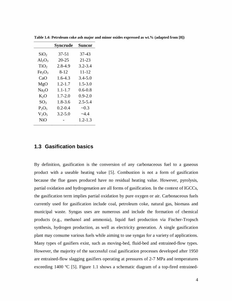
Table 1.4: Petroleum coke ash major and minor oxides expressed as wt.% (adapted from [8])

Syncrude Suncor

SiO2 37-51 37-43 Al2O3 20-25 21-23 TiO2 2.8-4.9 3.2-3.4 Fe2O3 8-12 11-12 CaO 1.6-4.3 3.4-5.0 MgO 1.2-1.7 1.5-3.0 Na2O 1.1-1.7 0.6-0.8 K2O 1.7-2.0 0.9-2.0 SO3 1.8-3.6 2.5-5.4 P2O5 0.2-0.4 ~0.3 V2O5 3.2-5.0 ~4.4 NiO - 1.2-1.3

1.3 Gasification basics

By definition, gasification is the conversion of any carbonaceous fuel to a gaseous

product with a useable heating value [5]. Combustion is not a form of gasification

because the flue gases produced have no residual heating value. However, pyrolysis,

partial oxidation and hydrogenation are all forms of gasification. In the context of IGCCs,

the gasification term implies partial oxidation by pure oxygen or air. Carbonaceous fuels

currently used for gasification include coal, petroleum coke, natural gas, biomass and

municipal waste. Syngas uses are numerous and include the formation of chemical

products (e.g., methanol and ammonia), liquid fuel production via Fischer-Tropsch

synthesis, hydrogen production, as well as electricity generation. A single gasification

plant may consume various fuels while aiming to use syngas for a variety of applications.

Many types of gasifiers exist, such as moving-bed, fluid-bed and entrained-flow types.

However, the majority of the successful coal gasification processes developed after 1950

are entrained-flow slagging gasifiers operating at pressures of 2-7 MPa and temperatures

exceeding 1400 ºC [5]. Figure 1.1 shows a schematic diagram of a top-fired entrained-

5

flow slagging gasifier. Generally, fuel is fed to the gasifier with oxygen, air and/or steam.

The fuel ash forms a relatively inert silicate melt (i.e., slag) which flows out the bottom

of the gasifier. The product stream is synthesis gas, also called syngas, which is mainly

rich in hydrogen and carbon monoxide, but also contains carbon dioxide, methane and

steam [9]. Additionally, particulate matter (fly ash and unconverted char) and undesired

sulphur and nitrogen compounds may be present in the syngas.

Figure 1.1: Schematic diagram of top-fired entrained-flow slagging gasifier.

Slag and quench water discharge

Syngas Quench water

Slag tap

Slag layer

Oxygen Fuel

>1400°C

<1000°C

6

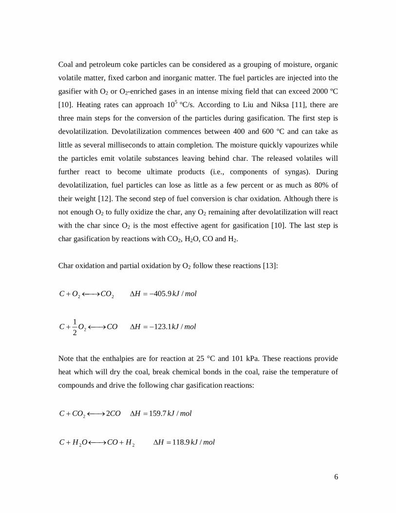
Coal and petroleum coke particles can be considered as a grouping of moisture, organic

volatile matter, fixed carbon and inorganic matter. The fuel particles are injected into the

gasifier with O2 or O2-enriched gases in an intense mixing field that can exceed 2000 ºC

[10]. Heating rates can approach 105 ºC/s. According to Liu and Niksa [11], there are

three main steps for the conversion of the particles during gasification. The first step is

devolatilization. Devolatilization commences between 400 and 600 ºC and can take as

little as several milliseconds to attain completion. The moisture quickly vapourizes while

the particles emit volatile substances leaving behind char. The released volatiles will

further react to become ultimate products (i.e., components of syngas). During

devolatilization, fuel particles can lose as little as a few percent or as much as 80% of

their weight [12]. The second step of fuel conversion is char oxidation. Although there is

not enough O2 to fully oxidize the char, any O2 remaining after devolatilization will react

with the char since O2 is the most effective agent for gasification [10]. The last step is

char gasification by reactions with CO2, H2O, CO and H2.

Char oxidation and partial oxidation by O2 follow these reactions [13]:

molkJHCOOC /9.40522

molkJHCOOC /1.12321

2

Note that the enthalpies are for reaction at 25 °C and 101 kPa. These reactions provide

heat which will dry the coal, break chemical bonds in the coal, raise the temperature of

compounds and drive the following char gasification reactions:

molkJHCOCOC /7.15922

molkJHHCOOHC /9.11822

7

molkJHCHHC /4.872 42

Moreover, equilibrium of the following gas phase reactions will dictate the product gas

composition:

molkJHCOHOHCO /9.40222

molkJHOHCHHCO /3.2063 242

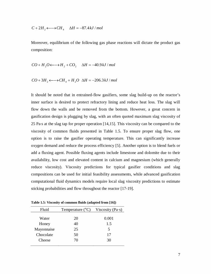
It should be noted that in entrained-flow gasifiers, some slag build-up on the reactor’s

inner surface is desired to protect refractory lining and reduce heat loss. The slag will

flow down the walls and be removed from the bottom. However, a great concern in

gasification design is plugging by slag, with an often quoted maximum slag viscosity of

25 Pas at the slag tap for proper operation [14,15]. This viscosity can be compared to the

viscosity of common fluids presented in Table 1.5. To ensure proper slag flow, one

option is to raise the gasifier operating temperature. This can significantly increase

oxygen demand and reduce the process efficiency [5]. Another option is to blend fuels or

add a fluxing agent. Possible fluxing agents include limestone and dolomite due to their

availability, low cost and elevated content in calcium and magnesium (which generally

reduce viscosity). Viscosity predictions for typical gasifier conditions and slag

compositions can be used for initial feasibility assessments, while advanced gasification

computational fluid dynamics models require local slag viscosity predictions to estimate

sticking probabilities and flow throughout the reactor [17-19].

Table 1.5: Viscosity of common fluids (adapted from [16])

Fluid Temperature (°C) Viscosity (Pa·s)

Water 20 0.001 Honey 40 1.5

Mayonnaise 25 5 Chocolate 50 17

Cheese 70 30

8

1.4 Research objectives and outline

The ultimate goal of this doctoral research program is the optimization of the design and

operation of gasifiers, particularly entrained-flow gasifiers running on Canadian fuels. Of

the many aspects involved in gasification, slagging is of great interest since it can

drastically alter operation and even completely halt it. Unfortunately, slagging behaviour

is still ill-understood due to modeling difficulties and limited data. As a result, the three

objectives advanced by this doctoral thesis specifically consider data collection and

modeling related to slagging in order to improve the accuracy of already developed and

soon-to-be developed comprehensive gasifier models.

The first objective is to develop slag viscosity models which are applicable to Canadian

fuels. Many models are available but their predictive power is poor unless they are

applied to specific fuels and conditions. Work has been done to improve these models

and new approaches, such as the application of artificial neural networks and

thermodynamic equilibrium, have been tested. Still, all slag viscosity models are

empirical or semi-empirical and therefore rely on slag viscosity measurements. For a

model to appropriately describe the viscosity of a given slag, it is imperative that such a

slag’s composition and temperature fall within the range of compositions and

temperatures used to produce the model. Although many viscosity values are available

for many slag compositions and temperatures with various fluxing agents, few values are

available for slags resulting from gasification of Canadian fuels and fluxing agents.

Hence the second objective is to perform slag viscosity measurements pertinent to

Canadian gasification fuels and fluxing agents. In particular, the effect of vanadium in

petroleum coke is examined. The third objective is to collect pilot plant data which will

lead to a better understanding of slagging while also providing data which can be used for

gasifier model validation.

Chapter 2 is a literature review of inorganic matter transformation sub-models for

entrained-flow slagging gasifiers. This chapter highlights the complexities of modeling

slag formation and flow in gasifiers. Sub-models for ash particle formation, gas-particle

9

transport, particle sticking, slag flow and slag-refractory interactions are presented and

discussed. The importance of slag viscosity should be apparent after reading this chapter.

Chapter 3 describes the development of artificial neural networks to model slag

viscosities over a broad range of temperatures and compositions. Chapter 4 presents tools

developed to assess various slag viscosity models. These tools include a slag viscosity

prediction calculator with 24 slag viscosity models, and a database of 4124 slag viscosity

measurements. Chapter 5 describes results of a slag viscosity measurement program for

slags produced from coal and petroleum coke blends. Additional details of the viscosity

measurement setup assembled at CanmetENERGY for this program are provided in

Appendix A. Chapter 6 describes interactions between petroleum coke slags and various

crucible materials used for slag viscosity measurements. Chapter 7 is a Canadian fuel

characterization study specifically designed to provide information required for modeling

inorganic matter transformations in gasifiers. Chapter 8 presents results from five pilot

scale gasification tests performed with the fuels characterized in the previous chapter.

The final chapter recaps the major conclusions and includes a discussion on

recommended future work to be conducted.

1.5 References

[1] Brown CE. World Energy Resources, 1st edition. Springer-Verlag: New York, 2002.

[2] Johnson J. Getting to ‘Clean Coal’. Chemical and Engineering News

2004;82(08):20-5.

[3] Hawkins DG, Lashof DA, Williams RH. What to do about coal. Scientific American

2006;295(3):68-75.

[4] Epcor. Genesee IGCC Project Backgrounder. www.epcor.ca, 2008.

[5] Higman C, van der Burgt M, (Eds.). Gasification, 2nd edition. Gulf Professional

Pub./Elsevier Science: Boston, 2008.

10

[6] Speight JG. Handbook of coal analysis. John Wiley & Sons, Inc.: Hoboken, 2005.

[7] Coal Association of Canada. Coal basics. www.coal.ca, 2012.

[8] Furimsky E. Gasification of oil sand coke: Review. Fuel Processing Technology

1998;56:263-90.

[9] Takematsu T, Maude C. Coal gasification for IGCC power generation. IEA Coal

Research 1991;37.

[10] Niksa S, Liu G, Hurt RH. Coal conversion submodels for design applications at

elevated pressures. Part I. Devolatilization and char oxidation. Progress in Energy and

Combustion Science 2003;29:425-77.

[11] Liu G, Niksa S. Coal conversion submodels for design applications at elevated

pressures. Part II. Char gasification. Progress in Energy and Combustion Science

2004;30:679-717.

[12] Smoot LD, Smith PJ. Coal combustion and gasification. Plenum Press: New York,

1985.

[13] Kristiansen A. Understanding coal gasification. IEACR report 86, 1996.

[14] Browning GJ, Bryant GW, Hurst HJ, Lucas JA, Wall TF. An empirical method for

the prediction of coal ash slag viscosity. Energy and Fuels 2003;17:731-7.

[15] Folkedahl BC, Schobert HH. Effects of atmosphere on viscosity of selected

bituminous and low-rank coal ash slags. Energy and Fuels 2005;19:208-15.

[16] Lindeburg MR. Mechanical Engineering Reference Manual for the PE Exam. 12th

edition. Professional Publications, Inc: Belmont, 2006.

[17] Seggiani M. Modelling and simulation of time varying slag flow in a Prenflo

entrained-flow gasifier. Fuel 1998;77:1611-21.

11

[18] Rushdi A, Gupta R, Sharma A, Holcombe D. Mechanistic prediction of ash

deposition in a pilot-scale test facility. Fuel 2005;84:1246-58.

[19] Wang XH, Zhao DQ, He LB, Jiang LQ, He Q, Chen Y. Modeling of a coal-fired

slagging combustor: Development of a slag submodel. Combustion and Flame

2007;149:249-60.

12

Chapter 2. Literature review of inorganic matter transformation sub-models for entrained-flow slagging gasifiers

2.1 Introduction

After volatilization, char combustion and char gasification, what is left of the coal

particles is mostly inorganic matter. Mineral classes present in coal include (in general

order of abundance) silicates, carbonates, oxyhydroxides, sulphides, sulphates,

phosphates and others [1]. Descriptions, images and chemical characteristics of minerals

are available online [2]. The fate of the inorganic matter in a gasifier can take one of two

directions. The first is entrainment by the gas phase where the inorganic matter leaves the

gasifier as fly ash. In this case, it must be removed by some particle removal process

prior to downstream processing of the gas. Alternatively, the fly ash may stick to the

gasifier walls, flow down and exit the bottom as a highly viscous by-product named slag.

This process has many implications as the slag can greatly affect heat transfer in the

system, corrode/protect the refractory lining of the gasifier, and even plug the gasifier

thus halting its operation. Hence there is much interest in predicting how the iorganic

matter will behave when designing and operating a gasifier.

Many qualitative indices have been devised to quickly and easily predict ash

slagging/fouling in combustion and gasification systems. Some are simply based on X-

ray fluorescence ash analysis (ASTM D 3174), such as the base-to acid ratio [3]:

232322

22

TiOOFeOAlSiOFeOMgOCaOOKONa

AcidBase

13

where chemical formulas denote molar fractions. A low ratio hints towards a higher

melting point and viscosity; hence a greater likelihood of gasifier plugging. Some indices

are based on more complex coal ash analyses such as ash fusion temperatures (AFTs)

(ASTM D 1857) or even computer controlled scanning electron microscopy (CCSEM)

data. Gupta [4] and van Alphen [5] provide good reviews of various coal characterization

techniques including AFTs and CCSEM. The University of North Dakota Energy and

Environmental Research Centre (UNDEERC) analysed bench, pilot and industrial scale

data to develop indices for slagging and fouling in power plants [6]. However,

slagging/fouling indices do not account for the multiple chemical and physical

phenomena coal ash experiences. As a result, they may provide misleading results and

are often limited to specific fuels and reactor designs [7,8].

Hence to obtain reliable quantitative predictions for inorganic matter transformations and

interactions within a gasifier, various inorganic matter phenomena must be studied in

detail with models describing each. In this review, inorganic matter phenomena in

gasifiers are grouped as follows; ash particle formation, gas-particle transport, particle

sticking, slag flow and slag-refractory interactions. Note that much of the available data

and models are from/for combustion systems, but are still applicable (sometimes with

slight modifications) to gasification.

2.2 Ash particle formation

As the water, volatiles and carbon are removed from a coal particle, the resulting ash

inorganic matter may coalesce, remain separate or even fragment. Ash particles produced

by combustion or gasification of a given coal display an array of sizes and compositions

[9]. Bulk coal ash analyses are inadequate indicators for ash particle formation since

differences in individual particle size and composition have a strong influence on particle

behaviour and must be accounted for [8]. For instance, ash is formed by inorganic

material in coal which can be associated to the carbon matrix in the form of minerals

14

embedded in the carbon matrix (included minerals), or in the form of minerals outside of

the carbon matrix (excluded minerals) [9-12]. Inorganic material may also be organically-

bound in the carbon matrix. These are mainly alkali and alkaline earth metals. They are

often grouped with included minerals or neglected, particularly with high rank coals

which tend to have little organically associated inorganics. The manner in which an

inorganic component is present in coal has a huge impact on its fate in gasification. The

dimensions of the minerals and coal particles also have a considerable impact. It is

impossible to characterize and track every single particle entering the gasifier. Therefore,

size, composition and association distributions must be determined in a statistically

meaningful manner. Two techniques used to determine these distributions are chemical

fractionation and CCSEM. Following a discussion on these techniques, models

describing ash particle formation are discussed.

2.2.1 Chemical fractionation and CCSEM

Chemical fractionation is a technique that provides information on the association of

inorganic species in coal using selective extraction based on solubility [4,13]. The

process consists of three successive extractions: (1) using water to remove water-soluble

salts; (2) using ammonium acetate to remove ion exchangeable elements; and (3) using

hydrochloric acid to remove acid-soluble species. Chemical fractionation is suitable for

quantification of type and abundance of organically associated inorganic species,

particularly in lower-rank subbituminous and lignitic coals which contain greater

amounts of these [9]. Doshi et al. [11] modified the chemical fractionation technique for

biomass fuels which also contain many organically bound inorganic species.

CCSEM can provide distribution of coal particle size, coal particle type, mineral particle

size, mineral particle type and mineral particle association (i.e., included or excluded)

[4,5]. Some CCSEM systems can also detect, characterize and quantify organically bound

inorganics. It should be noted that in this discussion, “CCSEM” refers to techniques

which, in an automated fashion, utilize electron microscopy and X-ray signal detection

(i.e., CCSEM, QEMSCAN and MLA). A typical CCSEM analysis is as follows. Coal

15

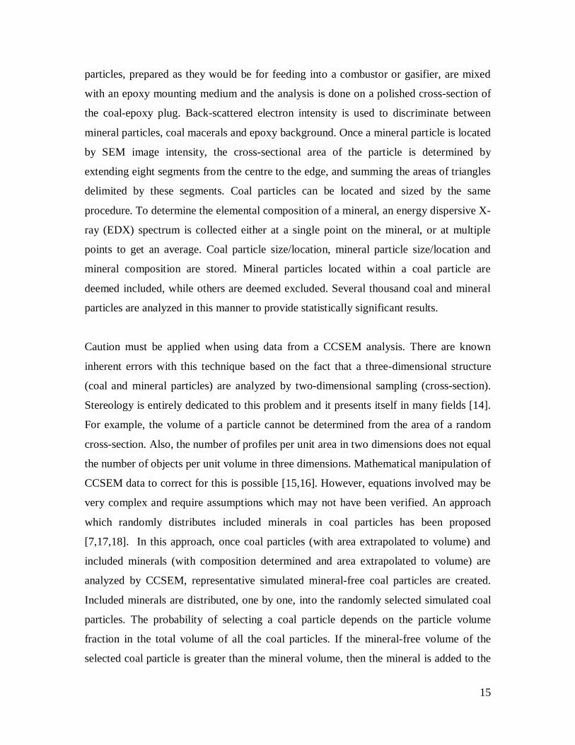
particles, prepared as they would be for feeding into a combustor or gasifier, are mixed

with an epoxy mounting medium and the analysis is done on a polished cross-section of

the coal-epoxy plug. Back-scattered electron intensity is used to discriminate between

mineral particles, coal macerals and epoxy background. Once a mineral particle is located

by SEM image intensity, the cross-sectional area of the particle is determined by

extending eight segments from the centre to the edge, and summing the areas of triangles

delimited by these segments. Coal particles can be located and sized by the same

procedure. To determine the elemental composition of a mineral, an energy dispersive X-

ray (EDX) spectrum is collected either at a single point on the mineral, or at multiple

points to get an average. Coal particle size/location, mineral particle size/location and

mineral composition are stored. Mineral particles located within a coal particle are

deemed included, while others are deemed excluded. Several thousand coal and mineral

particles are analyzed in this manner to provide statistically significant results.

Caution must be applied when using data from a CCSEM analysis. There are known

inherent errors with this technique based on the fact that a three-dimensional structure

(coal and mineral particles) are analyzed by two-dimensional sampling (cross-section).

Stereology is entirely dedicated to this problem and it presents itself in many fields [14].

For example, the volume of a particle cannot be determined from the area of a random

cross-section. Also, the number of profiles per unit area in two dimensions does not equal

the number of objects per unit volume in three dimensions. Mathematical manipulation of

CCSEM data to correct for this is possible [15,16]. However, equations involved may be

very complex and require assumptions which may not have been verified. An approach

which randomly distributes included minerals in coal particles has been proposed

[7,17,18]. In this approach, once coal particles (with area extrapolated to volume) and

included minerals (with composition determined and area extrapolated to volume) are

analyzed by CCSEM, representative simulated mineral-free coal particles are created.

Included minerals are distributed, one by one, into the randomly selected simulated coal

particles. The probability of selecting a coal particle depends on the particle volume

fraction in the total volume of all the coal particles. If the mineral-free volume of the

selected coal particle is greater than the mineral volume, then the mineral is added to the

16

coal particle and the mineral-free volume is adjusted. Otherwise, another coal particle is

selected. This continues until all included minerals have been placed in the simulated coal

particles. It is unclear whether the selection of a simulated coal particle is based on its

total volume or mineral-free volume. It may be more logical to base the selection on the

mineral-free volume. It is also unclear what is done if a mineral does not fit in any

mineral-free coal volume. This random attribution algorithm does require some

assumptions and does not correct all stereological errors. Other techniques may involve

sieving the coal to obtain a size distribution (although this also requires many unverified

assumptions). Laser diffraction may also be used to determine the particle size

distribution [19]. It may be necessary to also separate the particles by density if many

excluded minerals are present. Clearly, there is room for improvement in mineral and

coal characterization. Recent work applied computer tomography to determine the three-

dimensional shape of coal particles as well as the shape of included minerals [20]. This

and other new techniques will be required to obtain true size, composition and association

distributions.

2.2.2 Ash formation

When modeling the formation of ash, the mechanisms affecting included, excluded and

organically associated inorganics are quite different. First, for included inorganics, two

extreme ash particle formation models exist. The first is “full coalescence” which

assumes that all included minerals in a char particle coalesce together to form one ash

particle. The second is “no coalescence” which assumes that all included minerals in a

char particle remain separate and form separate ash particles. Unfortunately, for many

cases, neither extreme is applicable. Hence a partial coalescence model must be applied

[7,21]. The degree of coalescence is dependent upon the coal composition, coal particle

size distribution, the mineral matter distribution, char burnout mechanisms and char

fragmentation [22]. Different coal ranks with different macerals will form various types

of char particles [23]. During volatilization, softening and/or swelling of coal, combined

gases escaping will lead to the formation of pores and possibly an overall cenospheric

shape with a given wall thickness [18]. When it comes to modeling the formation of ash

17

particles from included inorganics, the following several basic assumptions are usually

made regarding the char structure and included mineral behaviour [16,18]: (1) The char

particles are spherical, either solid spheres or cenospheres with a uniform wall thickness.

(2) The char particles are consumed uniformly with the oxidation reaction only occurring

on the outer char surface, causing the outer surface to recede. (3) The included inorganics

are fully molten spheres which are randomly distributed throughout the char structure

with uniform probability based on char volume. Burning char is typically at a temperature

well above the melting point of typical minerals [22]. (4) Surface tension forces are

sufficient to keep the inorganic spheres on the char surface without movement. (5) There

are no miscibility limits or viscous flow resistances in coalescence.

As the char surface recedes, included inorganics on the outer surface of the char can

come into contact and coalesce with particles nearby on the surface, or beneath them

within the char. In the case of a cenospheric char particle, coalescence can proceed till the

centre void of the char particle is reached and the inorganic spheres are released. In the

case of a solid char particle, coalescence can proceed till all the char is reacted or

completely enveloped by inorganics (which results in one ash particle, agglomerating all

the included inorganics from that char particle). However, with both cenospheric and

solid char particles, the inorganic particles can be released during recession if they

encounter a char pore large enough to separate them from the char structure [18,22]. Char

pores range in size from Angstroms to tens of microns. However, only macropores (>1

micron) are of interest for ash release. To simplify the ash particle formation model, it is

possible to consider “ash separation length,” which is the average distance an inorganic

particle on the outer char surface recedes until it is separated from the char, either by

encountering a pore or the centre of the cenosphere [18,22]. Hence, in the ash particle

formation model, all char particles are assumed to be cenospheric without pores, and are

attributed an apparent wall thickness which represents the ash separation length. The

apparent wall thickness can be expressed as a percentage of the char particle diameter. A

char particle with high macroporosity and/or thin wall has a low apparent wall thickness

percentage. A solid char particle with low macroporosity has a high apparent wall

thickness percentage.

18

The char particle apparent wall thickness is generally an input to the ash particle

formation model. It may be determined through experimentation and/or based on coal

and char characterization. Char particles are often classified within one of three groups

[18,23]. Char Group I particles are thin-walled, cenospherical and contain a continuous

large cavity. Char Group III particles are solid with little or no void. Char Group II

particles have intermediate characteristics, with discontinuous voids of various sizes. Yan

et al. [18] associated apparent wall thicknesses of 5, 20 and 40% to Char Groups I, II and

III, respectively.

A simple ash formation model for included inorganics can be carried out as follows

[16,18]. Once simulated coal particles with included minerals are produced (which is

likely based on statistical data from CCSEM), the type of char (i.e., Char Group I, II or

III) particle formed is determined. Then based on the apparent char wall thickness (which

is related to the Char Group), inorganic particle sizes, coal particle sizes and inorganic

volume fractions in the coal, the probability of coalescence can be calculated. Monroe

[16] calculated the percent of included inorganics that coalesce, assuming various mono-

size and mono-density coal particles with mono-sized inorganic particles. These

calculations were done for various apparent char wall thicknesses. Yan et al. [18] related

these results to the char groups. Some other basic assumptions can be applied to the

inorganic matter, regardless if it is included or excluded; pyrite will release sulphur, clays

will release water and carbonates will release carbon dioxide [9,16]. Furthermore, ash

particles formed by included mineral coalescence will also include many organically

bound inorganics, although some of these organics may devolatilize and join the gas

phase [9,15,22]. Distribution of non-devolatilized organically bound inorganics added to

coalesced included minerals can be assumed proportional to the surface area of the ash

particles.

In literature, there are some variations to the above assumptions and model for included

inorganics. Barta et al. [15] uses a combustion model with shrinking core, down to a

certain radius (dependant on particle reactivity), after which the radius remains constant,

19

porosity increases and the char disintegrates. Instead of relating the ash particles to coal

particles, Baxter [24] characterized char particles to then model ash particle formation.

Lee and Lockwood [25] simplified their ash transformation model further by sampling

and characterizing fly ash directly.

Modeling the formation of ash particles from excluded inorganics is simpler than with

included inorganics. Excluded inorganics can either stay intact to form one ash particle

each, or fragment to form multiple ash particles. Fragmentation can be caused by thermal

shock at mineral surfaces and rapid gas formation and release from inside the inorganic

particles [18]. Benson et al. [9] mention that their model applies experimentally

determined fragmentation values for pyrite, pyrrhotite, oxidized pyrrhotite, Ca-Al-P,

kaolinite, montmorillonite, gypsum, barite, calcite, dolomite and iron carbonate. Yan et

al. [18] use a Poisson distribution to describe the fragmentation of excluded minerals. It

was assumed that all particle offsprings have the same size. Fragmentation was neglected

for some major mineral species (quartz, illite, kaolinite, montmorillonite, siderite,

ankerite). Collisions between coal/char particles, excluded inorganics and ash particles

were neglected. However, this assumption may only be applicable to certain reactor types

and conditions.

Ash particle formation models have been compared to experimental data from various

combustion facilities [7,9,15,16,18,24]. In some cases, simple no-coalescence or full-

coalescence models compared well. In other cases, partial coalescence was required to

properly describe results. However, in some studies, even partial coalescence failed to

provide proper predictions. Some models were only good for ash particle size predictions

or ash composition predictions, but not both. It is important to note that all these

comparisons with experimental data are for combustion conditions. Very little literature

covers ash formation specifically in gasification conditions, hence the applicability of the

models to gasification may be doubtful. Some insight may be given by work done by Li

et al. [12]. They collected char particles at various stages of conversion which were

generated in a laminar entrained-flow reactor with temperatures and a gas atmosphere

simulating gasifier conditions. SEM images of particles generated at 1400 °C showed the

20

transformation of the mineral-carbon association. Minerals were melted throughout most

of the conversion process (indicated by droplet-shaped bright particles). Most minerals at

the char surface seemed to remain attached as there were not many liberated ash particles

observed when char was still present. As carbon was further consumed, more molten

inorganic droplets are present at the char surface. The droplets at the surface gained in

size at higher char conversion, and very large particles covered by inorganics could be

observed at very high carbon conversions (>90%). These observations suggest that many

of the assumptions in ash formation models are valid with gasification conditions.

Nonetheless, much more data with other types of coal are necessary.

2.3 Gas-particle transport

Transport of particles entrained by gas is well documented for various processes. For the

most part, the general concepts can be applied to the transport of coal, char and ash

particles in an entrained-flow gasifier. Hence, only a very basic overview of general

concepts is given here. More focus will be given to transport concepts for particles in a

gasifier (or combustor) near a reactor surface as this has a profound impact on the fate of

inorganic matter.

For gas-phase fluid mechanics, it is usually assumed that variables such as velocity,

pressure and density are continuous point functions. This is known as the continuum

hypothesis [26]. Of course continuums do not exist on a microscopic scale since mass is

concentrated at atomic nuclei. However, on a macroscopic scale, this hypothesis usually

holds and mass and momentum can be considered to be spread uniformly throughout a

given volume. The same cannot be said of particle or droplet phases. Conservation

equations of Eulerian form apply to continuous phases. On the other hand, Lagrangian

equations follow the trajectory of each particle or droplet individually, making it

impractical for continuous phases. A purely Eulerian framework can be used to describe

gas-particle flows. Alternatively, a Eulerian gas-phase description can be combined with

21

a Lagrangian particle phase description. Although fundamental laws usually apply to a

Lagrangian framework, the Reynolds transport theorem can be used to convert them to a

Eulerian framework. Smoot and Smith [26] provide a more thorough overview of this

subject.

One of the greatest challenges in describing flow inside a gasifier is to accommodate

turbulence. The problem is compounded by the presence of multiple phases. For practical

considerations, conservation equations must be modified to account for turbulence. The

k-ε two-equation closure model is often used in combustion and gasification models. Lee

and Lockwood [25] and Watanabe and Otaka [27] describe the flow dynamics and

particle transport equations used in their CFD models.

Once particles are brought near a surface in the reactor, they must deviate from the gas

flow field to come into contact with the wall. Mechanisms like inertial impaction,

thermophoresis and eddy impaction can provide the energy required to overcome the

flow field [8,13,25,28,29]. When contact with the surface is established, other forces will

determine whether the particle sticks to the surface or rebounds (see Section 2.4). Surface

deposition may also be directly from the gas phase, by condensation or chemical reaction.

Inertial impaction (including some turbulence effects) and thermophoresis are briefly

described below. Other means of surface contacting are not as well understood and could

be less significant. They are discussed in work by Baxter [13].

For larger particles (>1 µm), inertial impaction is the dominant mechanism [8,25].

Momentum normal to the surface, gained by particles from gas entrainment away from

the surface or from turbulence, must overcome the gas stream lines near the surface. The

Stokes number has been correlated to impaction efficiency [30]. Baxter [13] has

demonstrated that for ash particles flowing towards a boiler heat transfer tube in typical

combustion conditions, the effects of the laminar boundary layer around the tube,

thermophoresis and turbulence are negligible.

22

Effects of the laminar boundary layer and turbulence may not be neglected for inertial

impaction on flat plates in parallel flow [13]. Correlations relating impaction efficiency to

the Stokes number are available, but their validity is less certain than for inertial

impaction in cross-flow [13]. Note that in some instances, swirled tangential flow may be

promoted in the gasifier chamber to increase particle-wall collisions [29].

Thermophoresis causes particle transport due to local temperature gradients within the

gas and/or the particle. In general, the thermophoretic force acts in the direction opposite

to the temperature gradient. With cross flow over a tube, deposits from thermophoresis

are more evenly distributed and finer grained than inertial impaction deposits. Also, as an

insulating layer of particles builds up on the surface, the temperature gradient decreases

leading to less thermophoretic deposition [30]. Correlations describing thermophoresis

are given by Baxter [13]. However, Baxter states that the accuracy of these is

questionable.

In their combustion model, Yan et al. [21] consider inertial impaction for larger particles.

They consider Brownian diffusion and thermophoresis for finer particles. They divide the

gas flow field into three zones; the fully turbulent core, the buffer layer and the boundary

layer. Inertial impaction acts in all three zones, while Brownian diffusion and

thermophoresis only act in the boundary layer due to insufficient temperature gradients in

the other zones. Analogous to electrical resistances, the overall resistance of ash transport

is calculated by summing individual resistances. Details of the individual resistances are

given by Im and Chung [31].

2.4 Particle sticking

Several factors may affect particle sticking. These include particle/surface temperature

and composition (which relate to viscosity and interfacial tension), impaction angle,

impaction velocity and particle size.

23

One approach to determine the sticking probability calculates the kinetic energy of the

impacting particle and the energy dissipation at impact. If the particle has more kinetic

energy than the amount which can be dissipated by the collision, it is assumed that the

particle bounces off. Otherwise, it is assumed that the particle sticks. This approach is not

widely adopted as it is difficult to predict the amount of energy which can be dissipated

[30]. Mueller et al. [32] calculate the excess energy after impaction and assume the

particle sticks if the energy is null or negative. For this, they applied the dimensionless

Weber number (which compares kinetic energy of the particles and the interfacial tension

energy between the particles and the substrate) and Reynolds number. If the excess

energy is greater than zero, it is assumed that the particle rebounds. Surface tension of the

particle and contact angle between the particle and substrate are required for this model.

These values are not well defined for particles in combustion and gasification systems.

Yong [33] simply assumed sticking when both the particle and surface are liquid, and

rebounding when both are solid. When either the particle is solid and the surface is liquid,

or the particle is liquid and the surface is solid, the Weber number is applied. Rebounding

was predicted when this number exceeded 1. Otherwise sticking was predicted. However,

Yong states that the effect of the Weber number and interference of trapped particles for

further sticking should be studied more thoroughly. Ni et al. [34] used the Weber

number, Reynolds number and contact angle to calculate the excess rebound energy. A

particle is assumed to rebound if this energy is greater than zero, and it is assumed to

stick otherwise. Sensitivity analyses were done for surface tension, viscosity, contact

angle, impact angle and impact velocity.

Another approach to predicting sticking probability is to use a viscosity criterion. The

extent to which a liquid droplet deforms upon impact depends on its kinetic energy and

viscosity. If the particle and surface have similar surface energies per unit area (i.e., a

small equilibrium contact angle), a larger contact area results in a greater sticking

probability. A large contact area will be produced if the liquid particle’s viscosity is low.

Walsh et al.’s [28] sticking model is often applied, where the particle sticking probability

is given by:

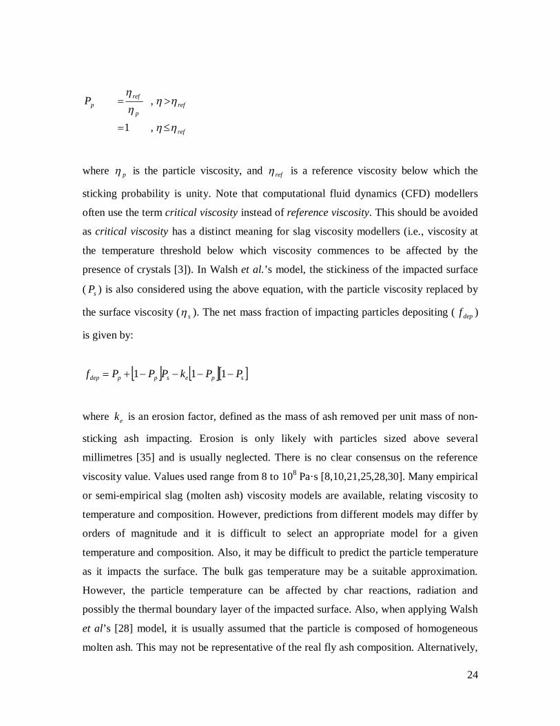
24

ref

refp

refpP

,1

,

where p is the particle viscosity, and ref is a reference viscosity below which the

sticking probability is unity. Note that computational fluid dynamics (CFD) modellers

often use the term critical viscosity instead of reference viscosity. This should be avoided

as critical viscosity has a distinct meaning for slag viscosity modellers (i.e., viscosity at

the temperature threshold below which viscosity commences to be affected by the

presence of crystals [3]). In Walsh et al.’s model, the stickiness of the impacted surface

( sP ) is also considered using the above equation, with the particle viscosity replaced by

the surface viscosity ( s ). The net mass fraction of impacting particles depositing ( depf )

is given by:

spesppdep PPkPPPf 111

where ek is an erosion factor, defined as the mass of ash removed per unit mass of non-

sticking ash impacting. Erosion is only likely with particles sized above several

millimetres [35] and is usually neglected. There is no clear consensus on the reference

viscosity value. Values used range from 8 to 108 Pa·s [8,10,21,25,28,30]. Many empirical

or semi-empirical slag (molten ash) viscosity models are available, relating viscosity to

temperature and composition. However, predictions from different models may differ by

orders of magnitude and it is difficult to select an appropriate model for a given

temperature and composition. Also, it may be difficult to predict the particle temperature

as it impacts the surface. The bulk gas temperature may be a suitable approximation.

However, the particle temperature can be affected by char reactions, radiation and

possibly the thermal boundary layer of the impacted surface. Also, when applying Walsh

et al’s [28] model, it is usually assumed that the particle is composed of homogeneous

molten ash. This may not be representative of the real fly ash composition. Alternatively,

25

Richter et al. [8] determined the viscosity of the six major mineral categories in the fly

ash they studied. The viscosity used to calculate the sticking probability for the fly ash

particles was based on a weight-averaged viscosity of the minerals.

For both the kinetic energy dissipation approach and the viscosity approach, small

particles are assumed to have a 100% sticking probability. One reason for this is that the

kinetic energy which must be dissipated is much smaller. Another reason is that the types

of forces bringing the particle to the surface may be different from inertial impaction. For

their energy dissipation model, Mueller et al. [32] recommend neglecting rebounding

with particles less than 75 µm. Moreover, Yan et al. [21] and Rushdi et al. [10] assumed

all particles less than 2-3 µm stick with their viscosity-based sticking models.

The viscosity sticking criteria used in many studies is applicable to ash particles with no

char remaining. However, if char is still present in the particle, the particle certainly will

not have a homogeneous composition and viscosity cannot be calculated. Li et al.

performed a series of experiments with partially converted char particles in a laminar

entrained-flow reactor under gasification conditions [12,36]. It was observed that up to a

certain char conversion (~90% for Illinois #6 coal), few particles were able to stick after

impaction onto an inclined plate. Past this critical conversion, almost all particles were

able to stick, provided they were at a temperature above the bulk ash flow temperature.

This critical conversion was related to the char-slag transition by SEM and surface area

analysis. The char-slag transition is when the porous non-sticky char transforms into non-

porous sticky slag. The low particle sticking before reaching the transition conversion

was attributed to excluded inorganics and liberated included inorganics. Hence a new

sticking criteria was developed, based on char conversion of the particles. This critical

conversion can be determined for a given coal by measuring the surface area of char

particles with various degrees of conversion. A significant drop in surface area should be

observed at and above the critical conversion.

Still, Li et al. used a bare plate for their sticking experiments. The char-slag transition

conversion may be useful to predict sticking during the initial use of a slagging gasifier or

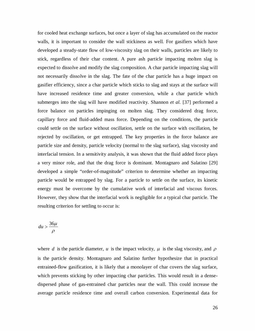
26

for cooled heat exchange surfaces, but once a layer of slag has accumulated on the reactor

walls, it is important to consider the wall stickiness as well. For gasifiers which have

developed a steady-state flow of low-viscosity slag on their walls, particles are likely to

stick, regardless of their char content. A pure ash particle impacting molten slag is

expected to dissolve and modify the slag composition. A char particle impacting slag will

not necessarily dissolve in the slag. The fate of the char particle has a huge impact on

gasifier efficiency, since a char particle which sticks to slag and stays at the surface will

have increased residence time and greater conversion, while a char particle which

submerges into the slag will have modified reactivity. Shannon et al. [37] performed a

force balance on particles impinging on molten slag. They considered drag force,

capillary force and fluid-added mass force. Depending on the conditions, the particle

could settle on the surface without oscillation, settle on the surface with oscillation, be

rejected by oscillation, or get entrapped. The key properties in the force balance are

particle size and density, particle velocity (normal to the slag surface), slag viscosity and

interfacial tension. In a sensitivity analysis, it was shown that the fluid added force plays

a very minor role, and that the drag force is dominant. Montagnaro and Salatino [29]

developed a simple “order-of-magnitude” criterion to determine whether an impacting

particle would be entrapped by slag. For a particle to settle on the surface, its kinetic

energy must be overcome by the cumulative work of interfacial and viscous forces.

However, they show that the interfacial work is negligible for a typical char particle. The

resulting criterion for settling to occur is:

36

du

where d is the particle diameter, u is the impact velocity, is the slag viscosity, and

is the particle density. Montagnaro and Salatino further hypothesize that in practical

entrained-flow gasification, it is likely that a monolayer of char covers the slag surface,

which prevents sticking by other impacting char particles. This would result in a dense-

dispersed phase of gas-entrained char particles near the wall. This could increase the

average particle residence time and overall carbon conversion. Experimental data for

27

char-slag interaction and effects on reactivity are emerging [38], but more needs to be

done.

2.5 Slag flow

Once the rate of ash deposition is known, slag flow down the walls of the gasifier can

also be characterized. The basic principles of slag flow are those of a falling film.

Momentum conservation can describe the velocity profile. Mass conservation must be

included to describe slag flowing in and out of a control volume, as well as the ash

sticking to the wall or being re-entrained by the gas phase. Since significant temperature

gradients will vary the slag properties, energy conservation must also be solved.

Consider the layer of slag built up on an inner gasifier wall in Figure 2.1. In this figure,

there is a single refractory wall layer for demonstrative purposes, although the wall can

be a combination of refractory materials, a water/gas cooling membrane and steel vessel

layers. The wall inclination ( ) is usually 90°, but can vary with different gasifier

configurations or sections. The slag layer is commonly divided in a liquid slag layer and a

solid slag layer. Here, these layers are more correctly termed immobile and flowing (as

solids and liquids can be present in both). The immobile layer is composed of slag which

is above a certain viscosity, rendering its mobility negligible. The temperature of critical

viscosity is often used to distinguish between the immobile and flowing slag layers

[33,39-41]. However, not all slags demonstrate a temperature of critical viscosity. It may

be more appropriate to use a direct viscosity criteria to distinguish between the immobile

and flowing layers (e.g., assume slag is immobile above 1000 Pa·s). Assuming the

presence of this layer does not simplify the slag flow model, but may be useful if there is

a significant change in slag properties (e.g., thermal conductivity) from the flowing layer

to the immobile layer. Nonetheless, in certain instances, there may be a flowing layer

without an immobile layer, or vice versa.

28

Figure 2.1: Schematic diagram of slag deposited on a gasifier wall.

Most slag flow models are based on the following momentum balance on a control

volume of slag (in Cartesian coordinates):

singr

29

where r is the distance from the slag-gas interface, is the shear stress, is the slag

density and g is gravitational acceleration. Shear stress is related to slag viscosity via

Newton’s law of viscosity:

ru

where is the slag viscosity, u is the slag velocity. Integrating and combining the two

equations above will give a velocity profile which is dependent on assumptions applied in

the model.

Bockelie et al. [40] developed a steady-state gasifier slag flow model with a numerical

solution. The model uses information from the gas flow field in the gasifier (gas

composition, gas temperature, incident heat transfer, particle deposition rate) to predict

slag properties (slag flow, slag thickness, immobile slag thickness) and heat transfer

through the gasifier walls. The following assumptions are applied. (1) The transition

temperature between the immobile and flowing slag layers is the temperature of critical

viscosity. (2) The flowing slag has Newtonian behaviour. (3) The shear stress between

the gas and slag layer is negligible. (4) The model is written in Cartesian coordinates with

a constant heat flux through the slag. This assumption is valid if the slag layer is thin

relative to the reactor diameter. (5) The heat transfer is normal to the surface. (7) The

density, specific heat and thermal conductivity of the slag are independent of

temperature.

Bockelie et al.’s model uses the following iterative procedure which starts from the top of

the gasifier. First, the thickness of the slag layer ( fit ) is assumed. At the top of

the gasifier, at y = 0, the slag layer thickness is defined to be zero. For y > 0, the slag

layer thickness at the previous axial position is used as an initial assumption for the

subsequent axial position. Then, using an iterative procedure based on radiation and

conduction equations, the surface temperature of the slag layer and the net heat flux to the

slag surface is calculated with:

30

S

wifgt q

TTk

where k is the slag’s thermal conductivity. fgT is the slag-gas interface temperature, wiT

is the wall-slag interface temperature, and Sq is the heat flux through the slag. The

velocity profile (at a given height) in the flowing slag layer is given by:

T

T

fg

S if

dT

qkgu

2

where u is the local slag velocity, is the slag density, T is the local temperature, is

the local slag viscosity, and is a dummy variable. ifT is a predetermined temperature

below which there is no slag flow. The mass flux of slag ( SM.

) at a given height is then

expressed as:

fg

if

T

TSS ud

qkM .

Then, the thickness of immobile slag ( i ) is calculated. The last step in the slag flow

model is to compare the mass flux of flowing slag with the ash deposition flux from the

gas. If these values agree within a reasonable tolerance (e.g., 0.1%), the assumed slag

layer thickness is correct and the calculations can be repeated at a lower section of the

gasifier until the bottom is reached. If the mass fluxes do not agree, then a new slag layer

thickness should be assumed and the calculations repeated for the gasifier section in

question.

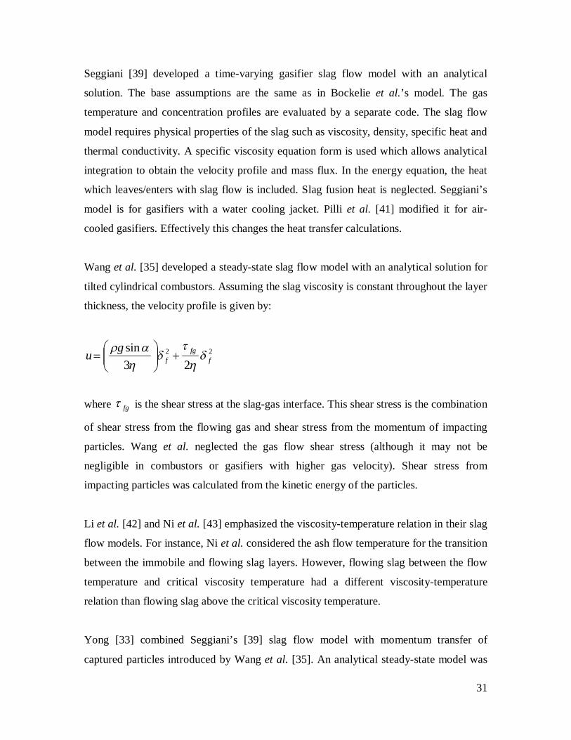
31

Seggiani [39] developed a time-varying gasifier slag flow model with an analytical

solution. The base assumptions are the same as in Bockelie et al.’s model. The gas

temperature and concentration profiles are evaluated by a separate code. The slag flow

model requires physical properties of the slag such as viscosity, density, specific heat and

thermal conductivity. A specific viscosity equation form is used which allows analytical

integration to obtain the velocity profile and mass flux. In the energy equation, the heat

which leaves/enters with slag flow is included. Slag fusion heat is neglected. Seggiani’s

model is for gasifiers with a water cooling jacket. Pilli et al. [41] modified it for air-

cooled gasifiers. Effectively this changes the heat transfer calculations.

Wang et al. [35] developed a steady-state slag flow model with an analytical solution for

tilted cylindrical combustors. Assuming the slag viscosity is constant throughout the layer

thickness, the velocity profile is given by:

22

23sin

ffg

fgu

where fg is the shear stress at the slag-gas interface. This shear stress is the combination

of shear stress from the flowing gas and shear stress from the momentum of impacting

particles. Wang et al. neglected the gas flow shear stress (although it may not be

negligible in combustors or gasifiers with higher gas velocity). Shear stress from

impacting particles was calculated from the kinetic energy of the particles.

Li et al. [42] and Ni et al. [43] emphasized the viscosity-temperature relation in their slag

flow models. For instance, Ni et al. considered the ash flow temperature for the transition

between the immobile and flowing slag layers. However, flowing slag between the flow

temperature and critical viscosity temperature had a different viscosity-temperature

relation than flowing slag above the critical viscosity temperature.

Yong [33] combined Seggiani’s [39] slag flow model with momentum transfer of

captured particles introduced by Wang et al. [35]. An analytical steady-state model was

32

produced by developing an energy balance for the reactor wall and slag layers.

Furthermore, the linear temperature profile assumed by Seggiani was replaced by a cubic

temperature profile. However, slag properties, including viscosity, are treated as

constants in the flowing slag layer.

Validation of slag flow models is extremely limited. One reason for this is that gasifier

vendors and the user community are very protective with information on process design

and operation, limiting the data available publicly [44]. Another reason is that

experimental data near the slag layer are very difficult to obtain due to harsh conditions

in gasifiers [33,35]. An alternative may be to validate slag flow models indirectly with

outer wall temperatures and heat loss to a coolant since slag buildup affects heat transfer

to the reactor walls. The slag mass flow rate exiting the gasifier may also be a useful

indicator. Li et al. [42] performed a quench of their pilot-scale gasifier at the end of a run

and measured the slag layer thickness at four locations. Values ranged from 6.38-6.81

mm, while their slag flow model prediction was 6.21 mm at these locations. Obviously

much more data of this type are needed for proper validation.

Many aspects of current slag flow models can be improved. All models mentioned above

assume a thin slag layer (relative to the reactor radius) allowing the use of Cartesian

coordinates. However, the slag layer is not always thin and there is much interest in

simulating cases where the reactor plugs or is nearly plugged due to slag buildup. Hence,

it may be necessary to use cylindrical coordinates, starting with the momentum continuity

equation. Moreover, some models provide an analytical solution while others provide a

numerical scheme. The advantage of an analytical solution may be apparent, such as

faster simulation due to lesser calculations, and an exact result provided the assumptions

are valid. On the other hand, a numerical solution may provide more flexibility with

various parameters and limit the assumptions required. For example, Seggiani’s model

discussed above requires a viscosity-temperature equation which can be integrated and

the overall model can change significantly if another viscosity-temperature equation is

used. As for choosing between a steady-state or transient slag flow model, the choice will

depend upon the specific application. Steady-state calculations are simpler, require fewer

33

assumptions, and may provide all the desired information. Conversely, some gasifier

operating conditions may never reach steady-state between start-up and shut-down.

Finally, various equations for specific phenomena will have to be added to the model to

accommodate various conditions. For example, some gasifiers operate with very high gas

flow rates and the shear stress on the slag surface is non-negligible. This will affect the

boundary conditions when solving the slag momentum balance and a gas shear stress

equation will have to be included.

2.6 Slag-refractory interactions

During operation, the inner walls of entrained-flow slagging gasifiers are exposed to

harsh conditions such as elevated temperature (as high as 1600°C), elevated pressure (20

bar or higher) and contact with corrosive and erosive gases, liquids and solids [45-47].

Furthermore, these parameters can vary significantly over the gasifier lifetime,

particularly during start-up and shut-down. Gasifiers are typically classified as having

either a refractory lining design or a water-cooled membrane design [48]. The refractory

lining design is simpler and less expensive. Refractories are usually alumina-based

(sintered and/or fused cast alumina-silicate, high alumina, chromia-alumina, chrome-

magnesia spinels, alumina-chromia-zirconia), provide good thermal insulation and low

energy losses [46]. However, their lifetime is usually only 3-30 months. Replacement

cost and downtime losses are significant. In comparison, membrane walls typically

consist of high-pressure tubes, in which steam is generated, covered by a castable

refractory (usually SiC) [48]. Ideally, a solid slag layer forms on the wall and protects it.

Good service life can be obtained (> 8 years). However, membrane walls are expensive

and experience more heat loss than refractory walls. Regardless of the type of wall used,

slag has a huge impact on the performance and lifetime of the wall. Basic slag-refractory

interaction concepts and models are discussed in the following. Note that the “refractory”

in question may be that of a refractory lining design, or a water-cooled membrane design.

34

Rawers et al. [45] lists eight mechanisms by which slag can degrade refractory: (1)

refractory dissolution; (2) refractory particles debonding; (3) slag-refractory elemental

replacement; (4) slag-refractory reaction producing new phases; (5) slag-refractory

physical mismatch; (6) slag penetration into refractory pores; (7) slag wear-abrasion-

erosion; (8) stress (and thermal cycle) loadings resulting in fragmentation and spallation.

Much of the experimental data studying these mechanisms derive from cup tests during

which slag is placed in cups of various refractory materials at relevant temperatures

[45,46]. After a given amount of time, the slag, refractory and slag-refractory interface

are analysed. Nakano et al. [49] and Park et al. [50] studied slag-refractory interactions

by sessile-drop type experiments using a confocal scanning laser microscope. Quenched

samples were analysed by scanning electron microscopy couple with energy-dispersive

X-ray spectroscopy (SEM-EDX).

Thermodynamic calculations are often relied upon to model refractory corrosion by slag.

Park et al. [50] used the thermodynamics software FactSage [51] to determine the amount

of CO and SiO gases formed via reaction between slag and a SiC refractory. Kovacik et

al. [52] used FACT (which is now part of the FactSage software package) to study the

dissolution of Cr2O3-Al2O3 refractory in various slags with various gas atmospheres. The

solubility limit of refractory in slag was predicted by progressively adding larger amounts

of refractory to the slag and gas until the slag could no longer incorporate more

chromium and chromium solids were stable at equilibrium. It was noted that the activity

of each phase, as calculated by FACT, can be used to calculate the thermodynamic

driving force of phase formation. Luz et al. [53] also used FactSage to predict slag-

refractory interactions. However, their focus was that of slag penetrating refractory. 100 g

of refractory were repeatedly added to the equilibrium liquid component of slag from the

previous step, thus modeling liquid slag transformation as it penetrates the refractory.

Predictions compared well to results from cup tests.

Still, degradation of refractory by interaction with slag is not solely a chemical process.

Many physical aspects play a key role. Lin et al. [54] developed a transient numerical

model for simulation of thermal stresses in a slag layer built up on a water-cooled

35

membrane wall. The effects of slag thickness and porosity were investigated. Johnson et

al. [55] developed a refractory degradation model using the finite element method to

predict the combined process of slag infiltration and spalling. The slag concentration field

in the refractory is solved incrementally so that effective diffusivity (determined

experimentally) can be input as a temperature-dependent quantity. The swelling strain

was defined as a linear function of the fractional slag concentration. The thermal strains

were based on a linear thermal expansion coefficient and the temperature change from an

initial reference temperature. The refractory elastic modulus, critical cracking stress, and

softening modulus (all three taken from literature) were used to predict refractory failure.

Various sensitivity analyses were performed. Model results vaguely compared well with

previously reported operation observations. Williford et al. [56] developed two models

for high-chromia refractory spalling in slagging gasifiers. The first model treats spalling

due to compressive forces caused by the volumetric expansion associated with the

replacement of chromium by slag-borne iron. As the slag penetrates the porous

refractory, an irregular diffusion front is established and slag iron reacts with refractory

chromium. The difference in growth strain between the slag-affected refractory and host

refractory leads to cracking and eventually spalling. The second model treats spalling due

to tensile forces caused by the volumetric shrinkage associated with chromium

volatilization and loss from the refractory matrix. Both models make use of slag effective

diffusivity, which in turn is a function of surface tension, contact angle and viscosity.

Williford et al. note that there are few quantitative models in the literature specifically

designed for prediction of gasifier refractory spalling, and even fewer quantative spalling

data. They suggest spall thickness as an indicator of spalling mechanism, since the

compressive stress model predicts a noticeably thicker spall (~4 cm) than the tensile

stress model (~1.3 cm).

Refractory failure alone is one of the greatest concerns for gasifier operators. Slag-

refractory interaction models are relatively new and will require many more studies.

Furthermore, interaction between slag and refractory should eventually be incorporated in

comprehensive gasifier models as some inputs for slag-refractory interaction models will

come from other sub-models, and vice versa. For example, dissolution of refractory

36

components in slag can greatly impact slag flow. Slag-refractory interaction models

presented above tend to either focus on corrosion (i.e., thermodynamic models) or

physical degradation (i.e., stress-induced spalling models). Close coupling of these two

approaches could lead to a far superior model. Experimental data for validation will be

crucial, despite technical difficulties such data collection may present.

2.7 References

[1] Vassilev SV, Vassileva CG. Occurrence, abundance and origin of minerals in coals

and coal ashes. Fuel Process Technol 1996;48:85-106.

[2] Barthelmy D. Mineralogy Database. www.webmineral.com, 2010.

[3] Vargas S, Straw and Coal Ash Rheology. Ph.D. thesis, Technical University of

Denmark, Denmark; 2001.

[4] Gupta R. Advanced coal characterization: A review, Energy & Fuels 2007;21:451-60.

[5] van Alphen C. Automated mineralogical analysis of coal and ash products -

Challenges and requirements. Minerals Eng 2007;20:496-505.

[6] University of North Dakota Energy and Environmental Research Center.

Development of Fireside Performance Indices - Task 8. Report DOE/MC/30098-5236,

1996.

[7] Wang H, Harb JN. Modeling of ash deposition in large-scale combustion facilities

burning pulverized coal. Progress in Energy and Combustion Science 1997;23:267-82.

[8] Richter S, Strohle J, Schnell U, Hein KRG. Application of the 3D combustion

simulation code AIOLOS to the prediction of ash deposition in a pulverised coal-fired

utility boiler. 4th International Symposium on Coal Combustion, Beijing, China, 1999.

37

[9] Benson SA, Hurley JP, Zygarlicke CJ, Steadman EN, Erickson TA, Predicting ash

behavior in utility boilers. Energy & Fuels 1993;7:746-54.



[11] Doshi V, Vuthaluru HB, Korbee R, Kiel JHA. Development of a modeling approach

to predict ash formation during co-firing of coal and biomass. Fuel Process Technol

2009;90:1148-56.

[12] Li S, Wu Y, Whitty KJ. Ash deposition behavior during char-slag transition under

simulated gasification conditions. Energy & Fuels 2010;24:1868-76.

[13] Baxter LL. Ash Deposit Formation and Deposit Properties: A Comprehensive

Summary of Research Conducted at Sandia's Combustion Research Facility. Sandia

report SAND2000-8253, 2000.

[14] Mouton PR. The History of Modern Stereology. www.disector.com, 2010.

[15] Barta LE, Toqan MA, Beér JM, Sarofim AF. Prediction of fly ash size and chemical

composition distributions: The random coalescence model. Symp Int Combust

1992;24:1135-44.

[16] Monroe LS. An experimental and modeling study of residual fly ash formation in

combustion of a bituminous coal. PhD thesis, Massachusetts Institute of Technology,

United States, 1989.

[17] Charon O, Sarofim AF, Beér JM. Distribution of mineral matter in pulverized coal.

Progress in Energy and Combustion Science 1990;16:319-26.

[18] Yan L, Gupta RP, Wall TF. A mathematical model of ash formation during

pulverized coal combustion. Fuel;81:337-44.

[19] Wedd MW. Determination of particle size distribution using laser diffraction.

http://www.erpt.org/, 2011.

38

[20] Masset PJ, Suhonen H. X-ray computer tomography on coal particles. 27th Annual

International Pittsburgh Coal Conference, Istanbul, Turkey, 2010.

[21] Yan L, Gupta RP, Wall TF. The implication of mineral coalescence behaviour on

ash formation and ash deposition during pulverised coal combustion. Fuel 2001;80:1333-

40.

[22] Kang S. Fundamental Studies of Mineral Matter Transformation during Pulverized

Coal Combustion: Residual Ash Formation. PhD thesis, Massachusetts Institute of

Technology, United States, 1991.

[23] Yu J, Lucas JA, Wall TF. Formation of the structure of chars during devolatilization

of pulverized coal and its thermoproperties: A review. Progress in Energy and


[24] Baxter LL. Char fragmentation and fly ash formation during pulverized-coal

combustion. Combust Flame 1992;90:174-84.

[25] Lee FCC, Lockwood FC. Modelling ash deposition in pulverized coal-fired

applications. Progress in Energy and Combustion Science 1999;25:117-32.

[26] Smoot LD, Smith PJ. Coal combustion and gasification. Plenum Press, New York,

1985.

[27] Watanabe H, Otaka M. Numerical simulation of coal gasification in entrained flow

coal gasifier. Fuel;85:1935-43.

[28] Walsh PM, Sayre AN, Loehden DO, Monroe LS, Beér JM, Sarofim AF. Deposition

of bituminous coal ash on an isolated heat exchanger tube: Effects of coal properties on

deposit growth. Progress in Energy and Combustion Science 1990;16:327-45.

[29] Montagnaro F, Salatino P. Analysis of char-slag interaction and near-wall particle

segregation in entrained-flow gasification of coal. Combust Flame 2010;157:874-83.

39

[30] Blanchard R. Measurements and modeling of coal ash deposition in an entrained-

flow reactor. MSc thesis, Brigham Young University, United States, 2008.

[31] Im KH, Chung PM. Particulate deposition from turbulent parallel streams. AICHE

Journal 1983;29:498-505.

[32] Mueller C, Selenius M, Theis M, Skrifvars B, Backman R, Hupa M, et al.

Deposition behaviour of molten alkali-rich fly ashes - Development of a submodel for

CFD applications. Proceedings of the Combustion Institute 2005;30(II):2991-8.

[33] Yong SZ. Multiphase models of slag layer built-up in solid fuel gasification and

combustion. MSc thesis, Massachusetts Institute of Technology, United States, 2010.

[34] Ni J, Yu G, Guo Q, Zhou Z, Wang F. Submodel for predicting slag deposition

formation in slagging gasification systems. Energy & Fuels 2011;25:1004-9.



2007;149:249-60.

[36] Li S, Whitty KJ. Investigation of coal char-slag transition during oxidation: effect of

temperature and residual carbon. Energy & Fuels 2009;23:1998-2005.

[37] Shannon GN, Rozelle PL, Pisupati SV, Sridhar S. Conditions for entrainment into a

FeOx containing slag for a carbon-containing particle in an entrained coal gasifier. Fuel

Process Technol 2008;89:1379-85.

[38] Zhao X, Zeng C, Mao Y, Li W, Peng Y, Wang T, et al. The surface characteristics

and reactivity of residual carbon in coal gasification slag. Energy & Fuels 2010;24:91-4.



40

[40] Bockelie MJ, Denison MK, Chen Z, Linjewile T, Senior C, Sarofim AF. CFD

modeling for entrained flow gasifiers in Vision 21 systems. www.reaction-eng.com,

2002.

[41] Pilli SP, Johnson KI, Williford RE, Sundaraman SK, Korolev VN, Crum JV.

Modeling of Time Varying Slag Flow in Coal Gasifiers. 25th Annual International

Pittsburgh Coal Conference, Pittsburgh, United States, 2008.

[42] Li X, Li G, Cao Z, Xu S. Research on flow characteristics of slag film in a slag

tapping gasifier. Energy & Fuels 2010;24:5109-15.

[43] Ni J, Zhou Z, Yu G, Liang Q, Wang F. Molten slag flow and phase transformation

behaviors in a slagging entrained-flow coal gasifier. Industrial and Engineering

Chemistry Research 2010;49:12302-10.

[44] Bockelie MJ, Denison MK, Chen Z, Senior C, Sarofim AF. Using models to select

operating conditions for gasifiers. www.reaction-eng.com, 2003.

[45] Rawers J, Kwong J, Bennett J. Characterizing coal-gasifier slag-refractory

interactions. Materials at High Temperatures 1999;16(4):219-22.

[46] Kinaev N. A review of mineral matter issues in coal gasification. Cooperative

Research Centre for Coal in Sustainable Development Report 60, www.ccsd.biz, 2006.

[47] Kwong K, Bennett J, Krabbe R, Thomas H, Powell C. Engineered Refractories for

Slagging Gasifiers. American Ceramic Society Bulletin 2006;85:17-20.

[48] Higman C, van der Burgt M, (Eds.). Gasification, 2nd edition. Gulf Professional

Pub./Elsevier Science, Amsterdam; Boston, 2008.

[49] Nakano J, Sridhar S, Bennett J, Kwong K, Moss T. Interactions of refractory

materials with molten gasifier slags. Int J Hydrogen Energy 2011;36:4595-604.

41

[50] Park JH, Park JG, Min DJ, Lee YE, Kang Y. In situ observation of the dissolution

phenomena of SiC particle in CaO-SiO2-MnO slag. Journal of the European Ceramic

Society 2010;30:3181-6.

[51] Bale CW, Pelton AD, Thompson WT, Eriksson G, Hack K, Chartrand P, et al.

FactSage. www.factsage.com, 2009.

[52] Kovacik GJ, Pelton AD, Degterov S. Thermodynamic calculation of

gas/slag/refractory equilibira in coal gasification. CanmetENERGY Report, Natural

Resources Canada, 1994.

[53] Luz AP, Martinez AGT, Braulio MAL, Pandolfelli VC. Thermodynamic evaluation

of spinel containing refractory castables corrosion by secondary metallurgy slag. Ceram.

Int. 2011;37:1191-201.

[54] Lin W, Liang Q, Yu G, Liu H, Gong X. Numerical modeling for non-steady thermal

stress analysis of slag layer in a membrane wall entrained-flow gasifier. Fuel

2011;90:2396-403.

[55] Johnson KI, Williford RE, Matyas J, Pilli SP, Sundaram SK, Korolev VN. Modeling

Slag Penetration and Refractory Degradation Using the Finite Element Model. 25th

Annual International Pittsburgh Coal Conference, Pittsburgh, United States, 2008.

[56] Williford RE, Johnson KI, Sundaram SK, Pilli SP. Models for Refractory Spalling in

Coal Gasifiers. 25th Annual International Pittsburgh Coal Conference, Pittsburgh, United

States, 2008.

42

Chapter 3. Artificial neural network model to predict slag viscosity over a broad range of temperatures and slag compositions Published in Fuel Processing Technology (2010) 91:8, p. 831-836

Marc A. Duchesnea, Arturo Macchia, Dennis Y. Lub, Robin W. Hughesb,

David McCaldenb, Edward J. Anthonyb

aChemical and Biological Engineering Department, University of Ottawa, 161 Louis

Pasteur, Ottawa, Ont., Canada, K1N 6N5

bCanmetENERGY, 1 Haanel Drive, Ottawa, Ontario, CANADA

43

3.1 Abstract

Threshold slag viscosity heuristics are often used for the initial assessment of coal

gasification projects. Slag viscosity predictions are also required for advanced

combustion and gasification models. An artificial neural network model was developed to

predict slag viscosity over a broad range of temperatures and slag compositions. This

model outperforms other slag viscosity models, resulting in an average absolute

logarithmic error of 0.703 when applied to validation data. Genesee coal ash viscosity

predictions were made to investigate the effect of adding Canadian limestone and

dolomite. The results indicate that magnesium in the fluxing agent provides a greater

viscosity reduction than calcium for the threshold slag tapping temperature range.

Keywords: Slag, Viscosity, Artificial neural network, Model

44

3.2 Introduction

Slag viscosity has major implications in metallurgical processes, coal combustion and

coal gasification. When coal is combusted or gasified at a sufficiently high temperature,

its ash component will form slag which can damage surfaces, reduce heat exchange and

create fouling. In entrained-flow slagging gasifiers, some slag build-up on the reactor’s

inner surface is desired to protect refractory lining and reduce heat loss. However, a great

concern in gasification design is plugging by slag, with an often quoted maximum slag

viscosity of 25 Pas for proper operation [1,2]. To ensure slag tappability, one option is to

raise the gasifier operating temperature, which can significantly increase oxygen demand

and overall cost, whereas another option is to blend fuels or add a fluxing agent. Possible

fluxing agents include limestone and dolomite due to their availability, low cost and

elevated content in calcium and magnesium, which generally reduce viscosity. Front-end

engineering and design (FEED) work is being conducted on a 270 MW Integrated

Gasification Combined Cycle (IGCC) power plant to be constructed in Alberta, Canada

[3]. For this work, 18 tonnes of Genesee coal were sent to the selected gasifier vendor to

test their technology with Albertan coal. Viscosity predictions for typical gasifier

conditions and slag compositions can be used for initial feasibility assessments, while

advanced combustion and gasification computational fluid dynamics models require local

slag viscosity predictions to estimate sticking probabilities and flow throughout the

reactor [4-6]. Since operating conditions and slag compositions can vary significantly not

only between processes, but also within a given process, an accurate viscosity model with

a wide range of applicability is desired. The objectives of this study are to develop and

apply such a model with a test coal ash, here Genesee coal ash, with varying amounts of

fluxing agents.

45

3.3 Slag viscosity

3.3.1 Parameters affecting viscosity

Like any fluid, slag rheology is a function of its molecular structure and dynamics. Slag

usually has silicon dioxide as its main component and can thus be categorized as a

silicate melt for which the random network model is often used to describe its rheology

[2,7]. According to this model, silicate melt components can be classified into three

categories; network formers, network modifiers and amphoterics. Network formers (e.g.,

Si4+ and Ge4+) stabilize the network and therefore increase viscosity. Network modifiers

(e.g., Na+, K+, Mg2+, Ca2+, Fe2+, Cr3+, V5+, Ba2+ and Sr2+) disrupt the network and

therefore decrease viscosity. Amphoterics (e.g., Al3+, Fe3+, B3+ and Zn2+) can act either as

network formers or modifiers. Although these general tendencies often hold true, the

actual phenomena is more complex leading to discrepancies between this description and

measured viscosities. Some discrepancies may be explained by changes in oxidation

level, changes in coordination, and phase separation. For instance, ferrous iron (Fe2+) is

considered to be a network modifier, while ferric iron (Fe3+) is considered to be

amphoteric. The oxidation state of iron will depend upon temperature, pressure and the

gaseous atmosphere above the slag [8]. Moreover, aluminum tends to be tetrahedrally

coordinated and act as a network former when its charge can be balanced by alkali metal

or alkaline earth metal cations [9]. If its charge is not balanced by a cation, it tends to be

hexahedrally coordinated and weaken the silicate melt structure.

Slag viscosity also has a strong dependence on temperature. At elevated temperatures,

slag acts as a Newtonian fluid and its viscosity usually decreases logarithmically with

increasing temperature. At lower temperatures, crystallization or the separation of

immiscible liquids may occur causing a dramatic increase in viscosity and non-

Newtonian behaviour.

Although there is no doubt that the atmosphere surrounding a silicate melt can impact its

viscosity [2,10], the relationship between the two is unclear. Under reducing conditions,

46

the viscosity at a given temperature is generally lower than in air. The effect seems to be

greater in silicate melts with high iron content, potentially due to a higher proportion of

iron in the ferrous state. The presence of water was also shown to lower or increase

viscosity depending on the melt’s composition.

Finally, the measurement technique can also affect the observed viscosity values. Vargas

et al. [7] reviewed various types of viscometers and concluded that rotational viscometers

are best suited for silicate melts mainly due to their range and accuracy. For this type of

viscometer, only the spindle and the crucible come into contact with the melt. Material

selection for these pieces is difficult since few materials can withstand the high

temperatures without contaminating the sample. Vargas et al. recommended that

platinum-rhodium be used for oxidizing or inert conditions, and molybdenum be used for

reducing or inert conditions.

3.3.2 Previous models

Most models developed to predict the viscosity of silicate melts are semi-empirical

models based on theoretical relations describing Newtonian fluids and relying on data

regression to obtain some empirical parameters. Example of these include the S2 [1], WF

[1], Urbain [11], Riboud [12] and KF [13] models. Vargas et al. [7] tested these and more

for silicate melts containing 20-75 mol% silicon dioxide, with temperatures in the range

of 1550-1900 K and measured viscosities between 0.01-10,000 Pas. Limited success was

obtained, with predictions often in error by several orders of magnitude. However,

Vargas et al. stated that for these tests, no attempt was made to maintain within the

compositional ranges for which the models were intended. Browning et al. [1] also

developed a semi-empirical model (BBHLW model) for Newtonian fluids in which it is

assumed that at a given viscosity the gradient of the viscosity-temperature curve is the

same for all coal slags. A linear regression was performed to obtain an equation relating

viscosity to a modified temperature. The modified temperature is the difference between

the actual temperature and a shift temperature, which is in turn correlated to composition

47

by an empirical equation. For coal and synthetic slags with viscosities less than 1000

Pas, their model outperformed the S2, KF and WF models.

Semi-empirical models relating the viscosity of non-Newtonian (heterogeneous) melts to

the viscosity of Newtonian (homogeneous) melts are also available [7]. For silicate melts,

non-Newtonian behaviour can be caused by the appearance of crystals in the melt, or the

separation of immiscible liquids. Most non-Newtonian models require knowledge of the

crystal fraction and sometimes crystal shape or size. F*A*C*T (now part of the

FactSageTM software package) can be used to determine phase fractions and compositions

for adjustment of the viscosity prediction [14]. Dyk et al. [15] employed FactSage to

estimate the composition of the liquid portion of heterogeneous slags and used this

composition in the KF model. It was stated that this method is highly likely to be more

accurate, but without providing quantitative details. Kondratiev and Jak [16] optimized

the Urbain model with experimental data of homogeneous melts as determined by

F*A*C*T. To calculate the viscosity of a heterogeneous slag, the proportion of solids and

the composition of the remaining liquid phase were first estimated using F*A*C*T, then

the liquid phase viscosity was calculated from the optimized Urbain model, and finally

this viscosity was adjusted depending on the volume fraction of solid particles, according

to the Roscoe equation (given in [16]). Again without giving quantitative details, it was

stated that good agreement was achieved between the model and over 4000 experimental

points. In sum, the integration of FactSage calculations when predicting slag viscosity

shows promise, but published quantitative comparison of predictions and experimental

values are lacking. Also, although the FactSage database is constantly expanding,

limitations may still exist with certain compositions where higher order interactions are

encountered.

Artificial neural networks (ANNs) are gaining popularity in various engineering domains.

They attempt to reproduce the functionality of the brain which consists of many

interconnected neurons functioning in parallel. Each neuron will receive signals of

varying intensities, process them, and accordingly send out a signal with a given intensity

to be processed by other neurons. ANNs present significant advantages over conventional

48

data regression models [17] as there is no need to provide a model function, the learning

capability of ANNs allows the discovery of more complex and subtle interactions

between variables, and ANNs are intrinsically more robust when it comes to handling

noisy or inaccurate data. In designing an ANN, it is important to consider the structure of

the network, as well as the learning algorithm used to train it. To train an ANN, sets of

inputs and corresponding outputs are provided, and the weights are initialized to random

values. Inputs are sequentially sent through the ANN and the error on the calculated

output is determined from the provided output sets, according to a specified performance

function. The weights of the signals are adjusted to minimize the error. The process is

repeated until a certain number of iterations are completed or a given error tolerance is

attained. Other stop criteria may be specified. The method by which weights are adjusted

depends on the learning algorithm. ANNs should be validated with data which was not

used for training in order to detect over-fitting. They are particularly prone to over-fitting

due to the large number of parameters used. Reviews covering various aspects of neural

network modeling are available in [17,18].

A literature search revealed two studies describing silicate melt viscosity modeling via

ANNs. The earliest attempt was based on 350 data points of magnesium-rich slags and

the developed ANN was shown to outperform a linear regression model, prepared by the

authors, which was based on the same data [19]. Hanao et al. [20] produced neural

networks for mould fluxes (a type of silicate melt) using data collected during a round

robin project involving 21 research groups. They compared their neural network

predictions with those of the Iida model [21] and stated that the neural networks

performed much better without providing quantitative details. However, comparisons

were made over a very small range (0-6 Pas) of viscosities. Although these two attempts

to model silicate melt viscosity by ANNs are promising, their range of applicability may

be highly constrained in terms of composition (magnesium-rich slags in the first study)

and viscosity (below 6 Pas in the second study). Hence, in this study it was desired to

develop a general slag viscosity model with a wide range of applicability.

49

3.4 Artificial neural network modeling of slag viscosity

3.4.1 Dataset and input variable selection

There are numerous silicate melt viscosity measurements available in the literature.

Unfortunately, the techniques used to obtain them vary greatly and the sources of

potential errors are numerous. In addition, many different components are found in

silicate melts and creating a model that accounts for all of them may be unrealistic. To

control some of the variability caused by experimental technique, all data used in this

study was obtained using a rotational viscometer, with the exception of viscosity data

from dataset U (see Table 3.1) in the range of 107 to 1012 Pas, which was obtained by a

falling film method. Although it would be desirable to also limit the selected datasets

according to spindle and crucible materials used, a great deal of data is required to create

an ANN with a wide range of applicability, and such material stringency would eliminate

too much data from the study. Nevertheless, the authors believe that the effect caused by

spindle/crucible contamination is negligible compared to the effect of the primary input

sources of the model. An attempt was made to account for atmosphere used during

measurements. None of the conventional regression models mentioned previously

directly account for the slagging atmosphere (or its pressure). Some may indirectly

account for atmosphere by differentiating ferric and ferrous iron, but this introduces

errors associated with determining the quantity of each ion present in the melt. With

neural networks, the atmosphere can be accounted for by one or more additional inputs.

A few trials were performed using an additional input to those listed below, with air

being attributed a value of 1, and nitrogen and argon a value of -1. Data that was not

obtained with one of these atmospheres, or for which the atmosphere is unknown, was

not used. Although one of the ANNs developed performed very well, when varying the

initial weights prior to training, the results obtained were inconsistent. This suggests that

there may be over-fitting. ANNs developed while limiting the data to one atmosphere had

poor performance, likely due to lack of data. For these reasons, atmosphere was not

controlled for the final ANN. Table 3.1 lists the datasets used in this study, the number of

50

data points in each, as well as the spindle/crucible material and atmosphere used for

measurements.

Table 3.1: Datasets used for ANN models in this study

Letter code Reference Material Atmosphere Data points

A Persson (2007) [22] Fe/Mo Ar 111 B Shankar et al. (2007) [23] Mo Ar 54 C Hurst et al. (2000) [24] Mo N2 51 D Hurst et al. (1999a) [25] Mo N2 105 E Hurst et al. (1999b) [26] Mo N2 170 F Hurst et al. (1996) [7] Mo N2 18 G Stein and Spera (1993a) [7] Al2O3 air 103 H Stein and Sperra (1993b) [7] Al2O3 air 7 I Nowok and Benson (1991) [7] unknown CO/CO2 12 J Dingwell (1989) [7] Pt/Rh air 23 K Dingwell and Virgo 1988 [7] Pt/Rh air 80 L Jones and Lindsey (1987) [7] unknown unknown 63 M Scarfe and Cronin 1986 [7] Pt/Rh unknown 42 N Vorres et al. (1986) [7] Al2O3/Mo H2/CO/N2, air 16 O Mysen et al. (1985) [7] Pt/Rh air 16 P Quon et al. (1985) [7] Mo unknown 106 Q Hochella and Brown (1984) [7] unknown unknown 6 R Seki and Oeter (1984) [7] Pt/Rh air, CO2 49 S Scarfe 1983 [7] Pt/Rh air 75 T Schobert et al. (1982) [7] C/Al2O3 H2/N2, N2, air 37 U Urbain et al. (1982) [7] Mo/W vacuum, Ar 482 V Piwinskii and Weed (1980) [7] unknown air 37 X Segers et al. (1979) [7] Pt/Rh Ar 18 Y Bodnar et al. (1978) [7] Fe/Pt N2 163

The inputs selected for the ANN are elemental mole fractions and temperature, in

kelvins, normalized as follows:

51

108227551082

etemperaturinputetemperatur

Oxygen and components which never exceed a mole fraction of 0.02 in the selected

datasets are not considered here. Mole fractions were normalized to have a sum of 1. The

ranges of each input when combining all datasets used are given in Table 3.2.

Table 3.2: Input and output ranges of ANN models in this study

Input/output Minimum Maximum Temperature (K) 1082 2755 Si mole fraction 0.13 1.00 Al mole fraction 0.00 0.82 Fe mole fraction 0.00 0.81 Ca mole fraction 0.00 0.60 Mg mole fraction 0.00 0.65 Na mole fraction 0.00 0.50 K mole fraction 0.00 0.51 Mn mole fraction 0.00 0.69 Log(viscosity (Pa·s)) -3.81 11.16

3.4.2 Performance function

The proper selection of the function which is minimized when adjusting the parameters

of a model, the performance function, is important. One performance function which is

commonly used is the average absolute error ( AAE ):

N

iii mp

NAAE

1

1

52

where ip is the thi predicted value and im is the thi measured value for N data points.

The trouble with using AAE is that errors for small values, which may be relatively

large, are summed with errors on large values. Usually there is a greater tolerance for

error (difference between the prediction and measurement) when values get larger. The

same problem is seen with the average squared error ( ASE ). To account for this greater

error tolerance on larger values, the average absolute relative error ( AARE ) is often

used:

N

i i

ii

mmp

NAARE

1

1

This will result in a value which is plus or minus a given percentage of the measured

value. Unfortunately, this function does not differentiate a positive relative error from a

negative relative error. For instance, the model user will likely prefer an error of +60%

(which yields a prediction which is off by a factor of 1.6) than an error of -50% (which

yields a prediction which is off by a factor of 2). The AARE performance function will

favour the inverse. Hence a performance function which gives an average factor

difference would be best. This is achieved by using the average absolute logarithmic error

( AALE ):

N

iii mp

NAALE

11010 loglog1

where, on average, the measured value is equal to the predicted value multiplied or

divided by 10 to the power of AALE . The average squared logarithmic error ( ASLE )

will yield similar results.

3.4.3 Architecture and training

ANNs were created using MATLAB® version 7.6 [27]. All ANNs tested were feed-

forward with back-propagation. Datasets C, D, L, P and X were used for validation

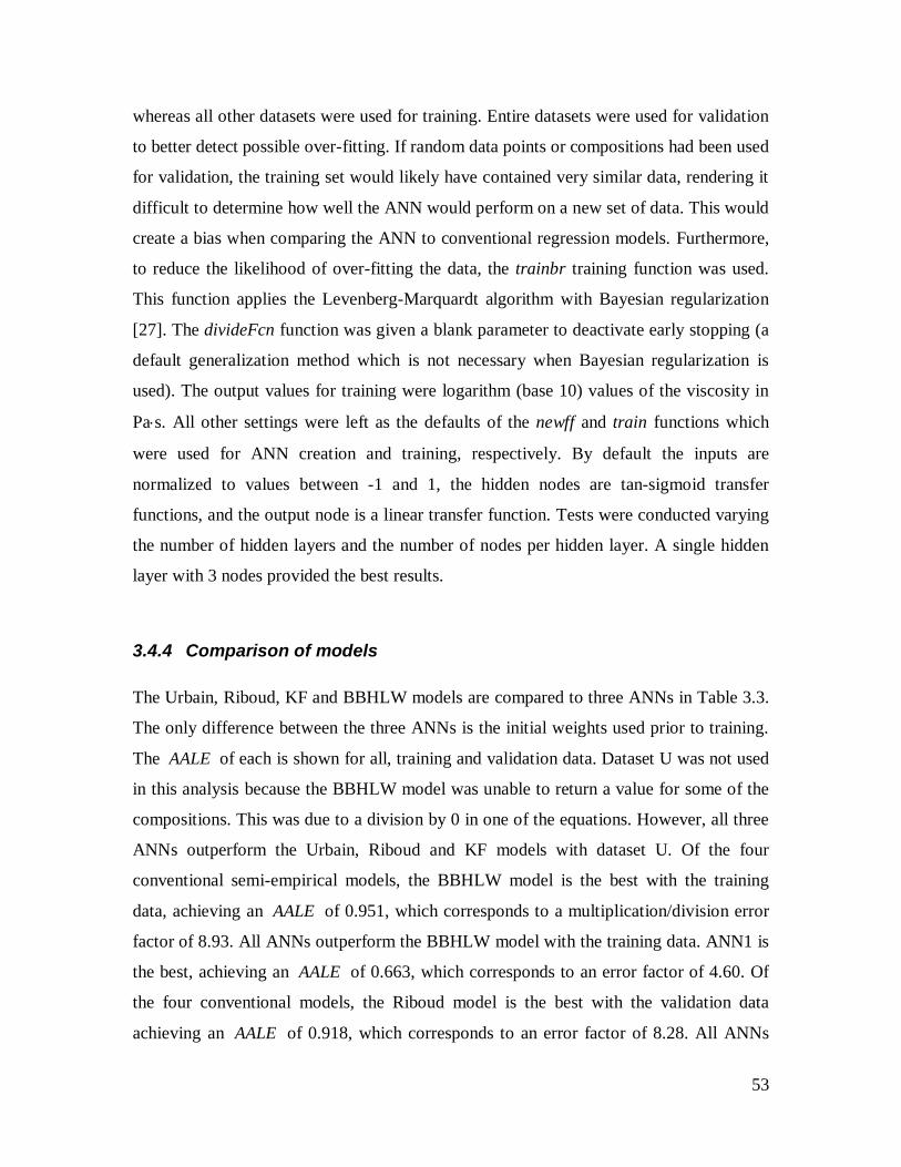
53

whereas all other datasets were used for training. Entire datasets were used for validation

to better detect possible over-fitting. If random data points or compositions had been used

for validation, the training set would likely have contained very similar data, rendering it

difficult to determine how well the ANN would perform on a new set of data. This would

create a bias when comparing the ANN to conventional regression models. Furthermore,

to reduce the likelihood of over-fitting the data, the trainbr training function was used.

This function applies the Levenberg-Marquardt algorithm with Bayesian regularization

[27]. The divideFcn function was given a blank parameter to deactivate early stopping (a

default generalization method which is not necessary when Bayesian regularization is

used). The output values for training were logarithm (base 10) values of the viscosity in

Pas. All other settings were left as the defaults of the newff and train functions which

were used for ANN creation and training, respectively. By default the inputs are

normalized to values between -1 and 1, the hidden nodes are tan-sigmoid transfer

functions, and the output node is a linear transfer function. Tests were conducted varying

the number of hidden layers and the number of nodes per hidden layer. A single hidden

layer with 3 nodes provided the best results.

3.4.4 Comparison of models

The Urbain, Riboud, KF and BBHLW models are compared to three ANNs in Table 3.3.

The only difference between the three ANNs is the initial weights used prior to training.

The AALE of each is shown for all, training and validation data. Dataset U was not used

in this analysis because the BBHLW model was unable to return a value for some of the

compositions. This was due to a division by 0 in one of the equations. However, all three

ANNs outperform the Urbain, Riboud and KF models with dataset U. Of the four

conventional semi-empirical models, the BBHLW model is the best with the training

data, achieving an AALE of 0.951, which corresponds to a multiplication/division error

factor of 8.93. All ANNs outperform the BBHLW model with the training data. ANN1 is

the best, achieving an AALE of 0.663, which corresponds to an error factor of 4.60. Of

the four conventional models, the Riboud model is the best with the validation data

achieving an AALE of 0.918, which corresponds to an error factor of 8.28. All ANNs

54

outperform the Riboud model with the validation data. ANN1 is the best, achieving an

AALE of 0.703, which corresponds to an error factor of 5.05. Overall, ANN1 has the

best performance and its final weight values are given in Table 3.4. For the ANNs, the

small difference in AALE between the training and validation sets, as well as between

each other, are indications of good generalization.

Table 3.3: Average absolute logarithmic errors of compared models for each dataset group

Dataset group Model All Training Validation

Urbain 1.164 1.191 1.083 Riboud 1.093 1.152 0.918 KF 1.134 1.182 0.992 BBHLW 0.954 0.951 0.964 ANN1 0.673 0.663 0.703 ANN2 0.734 0.699 0.837 ANN3 0.714 0.684 0.803

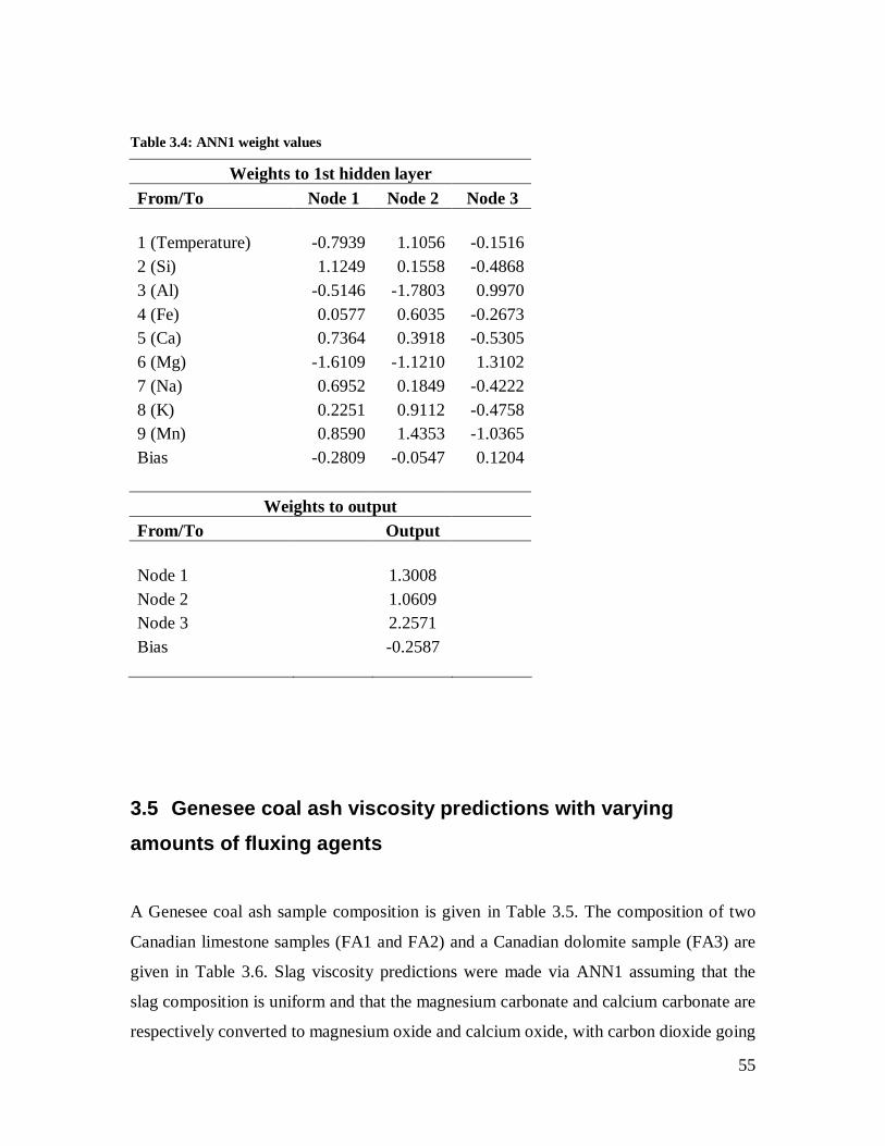
55

Table 3.4: ANN1 weight values

Weights to 1st hidden layer From/To Node 1 Node 2 Node 3 1 (Temperature) -0.7939 1.1056 -0.1516 2 (Si) 1.1249 0.1558 -0.4868 3 (Al) -0.5146 -1.7803 0.9970 4 (Fe) 0.0577 0.6035 -0.2673 5 (Ca) 0.7364 0.3918 -0.5305 6 (Mg) -1.6109 -1.1210 1.3102 7 (Na) 0.6952 0.1849 -0.4222 8 (K) 0.2251 0.9112 -0.4758 9 (Mn) 0.8590 1.4353 -1.0365 Bias -0.2809 -0.0547 0.1204

Weights to output From/To Output Node 1 1.3008 Node 2 1.0609 Node 3 2.2571 Bias -0.2587

3.5 Genesee coal ash viscosity predictions with varying amounts of fluxing agents

A Genesee coal ash sample composition is given in Table 3.5. The composition of two

Canadian limestone samples (FA1 and FA2) and a Canadian dolomite sample (FA3) are

given in Table 3.6. Slag viscosity predictions were made via ANN1 assuming that the

slag composition is uniform and that the magnesium carbonate and calcium carbonate are

respectively converted to magnesium oxide and calcium oxide, with carbon dioxide going

56

to the gas phase. Figures 3.1-3.3 show the effect of adding FA1-FA3, respectively. The

results suggest that if no fluxing agent is added, gasifier operation would have to be kept

above 1750 K to have the slag viscosity below the recommended maximum of 25 Pas.

Addition of 0.5 g FA1 per 1 g ash reduces the required temperature to ~1675 K, while

addition of 1 g FA1 per 1 g ash further decreases the required temperature to ~1600 K.

FA2 additions yield similar results, although the required temperatures are slightly

higher, likely due to greater silicon dioxide content. Conversely, the effect of FA3

addition is much more pronounced. Addition of 0.5 g FA3 per 1 g ash reduces the

required temperature to ~1500 K while addition of 1 g FA1 per 1 g ash further decreases

the required temperature to ~1350 K. FA1 and FA3 are very similar in composition

except for their calcium carbonate and magnesium carbonate fractions. Although they

have roughly the same amount of combined calcium carbonate and magnesium

carbonate, FA3 has much more magnesium carbonate. Hence, with this ash, magnesium

seems to be a better fluxing agent than calcium. Browning et al. [1] also predict a greater

viscosity reducing effect with magnesium than with calcium in their model. Furthermore,

the addition of FA3 seems to reduce the slag’s sensitivity to temperature at higher

temperatures, as can be seen by the reduction in slope with increasing temperature in

Figure 3.3. Consequently, if the viscosity threshold is set to a lower limit, or gasifier

operation is conducted at a higher temperature, addition of a magnesium-rich fluxing

agent may not be favourable. Finally, it must be stressed that these predictions should

only be taken as a preliminary basis for gasifier design while general trends are

investigated. ANN1 has an AALE of 0.703 for data it was not trained with, meaning that

the actual viscosity could easily be 5 times greater or smaller. Viscosity measurements

closer to the desired composition, temperature and atmosphere would provide

indispensable information.

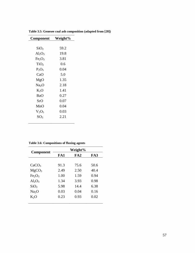
57

Table 3.5: Genesee coal ash composition (adapted from [28])

Component Weight%

SiO2 59.2 Al2O3 19.8 Fe2O3 3.81 TiO2 0.6 P2O5 0.04 CaO 5.0 MgO 1.35 Na2O 2.18 K2O 1.41 BaO 0.27 SrO 0.07 MnO 0.04 V2O5 0.03 SO3 2.21

Table 3.6: Compositions of fluxing agents

Weight% Component FA1 FA2 FA3

CaCO3 91.3 75.6 50.6 MgCO3 2.49 2.50 40.4 Fe2O3 1.00 1.59 0.94 Al2O3 1.34 3.93 0.98 SiO2 5.98 14.4 6.38 Na2O 0.03 0.04 0.16 K2O 0.23 0.93 0.02

58

-2

0

2

4

6

8

900 1100 1300 1500 1700 1900 2100Temperature [K]

Log

( vi

scos

ity [P

a·s]

)

0.0 g FA1 / g ash0.5 g FA1 / g ash1.0 g FA1 / g ash

Figure 3.1: Viscosity predictions for Genesee coal ash with varying amounts of FA1. The horizontal

hashed line corresponds to a viscosity of 25 Pa·s.

59

-2

0

2

4

6

8

900 1100 1300 1500 1700 1900 2100Temperature [K]

Log

( vi

scos

ity [P

a·s]

)




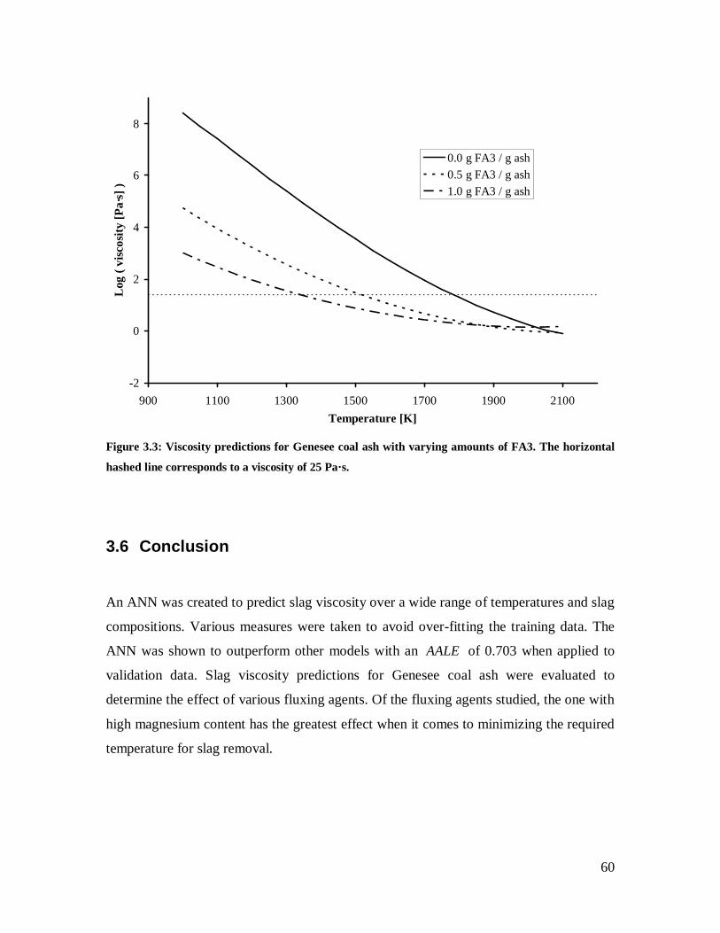
60

-2

0

2

4

6

8

900 1100 1300 1500 1700 1900 2100Temperature [K]

Log

( vi

scos

ity [P

a·s]

)




3.6 Conclusion

An ANN was created to predict slag viscosity over a wide range of temperatures and slag

compositions. Various measures were taken to avoid over-fitting the training data. The

ANN was shown to outperform other models with an AALE of 0.703 when applied to

validation data. Slag viscosity predictions for Genesee coal ash were evaluated to

determine the effect of various fluxing agents. Of the fluxing agents studied, the one with

high magnesium content has the greatest effect when it comes to minimizing the required

temperature for slag removal.

61

3.7 Acknowledgements

The authors are grateful to the Natural Sciences and Engineering Research Council of

Canada for financial assistance.

3.8 References

[1] Browning GJ, Bryant GW, Hurst HJ, Lucas JA, Wall TF. An empirical method for the

prediction of coal ash slag viscosity. Energy and Fuels 2003;17:731-7.



[3] Epcor, Genesee IGCC Project Backgrounder, www.epcor.ca, 2008.







2007;149:249-60.

[7] Vargas S, Straw and Coal Ash Rheology. Ph.D. thesis, Technical University of

Denmark, Denmark; 2001.

[8] Virgo D, Mysen BO. The structural state of iron in oxidized vs. reduced glasses at 1

atm: A57Fe Mo ̈ssbauer study. Physics and Chemistry of Minerals 1985;12:65-76.

62

[9] Goto A, Oshima H, Nishida Y. Empirical method of calculating the viscosity of

peraluminous silicate melts at high temperatures. Journal of Volcanology and Geothermal

Research 1997;76:319-27.

[10] Schobert HH, Streeter RC, Diehl EK. Flow properties of low-rank coal ash slags.

Implications for slagging gasification. Fuel 1985;64:1611-17.

[11] Urbain G, Cambier F, Deletter M, Anseau MR. Viscosity of silicate melts.

Transactions & Journal of the British Ceramic Society 1981;80:139-41.

[12] Riboud PV, Roux Y, Lucas LD, Gaye H. Improvement of continuous casting

powders. Fachber. Hüttenprax. Metallweiterverarb 1981;19:859-69.

[13] Kalmanovitch DP, Frank M. An effective model of viscosity for ash deposition

phenomena. In Mineral Matter and Ash Deposition from Coal. Bryers RW, Vorres KS

(Eds.), United Engineering Trustees, Inc., New York; 1990, p. 89–102.


FactSage. www.factsage.com, 2009.

[15] van Dyk JC, Waanders FB, Benson SA, Laumb ML, Hack K, Viscosity predictions

of the slag composition of gasified coal, utilizing FactSage equilibrium modelling. Fuel

2009;88:67-74.

[16] Kondratiev A, Jak E. Predicting coal ash slag flow characteristics (viscosity model

for the Al2O3-CaO-'FeO'-SiO2 system). Fuel 2001;80:1989-2000.

[17] Meireles MRG, Almeida PEM, Simões MG. A comprehensive review for industrial

applicability of artificial neural networks. IEEE Transactions on Industrial Electronics

2003;50:585-601.

[18] Jain AK, Mao J, Mohiuddin KM. Artificial neural networks: A tutorial. Computer

1996;29:31-44.

63

[19] Saxén H, Zhang X. Neural-network based model of blast furnace slag viscosity.

Proceedings of the International Conference on Engineering Application of Neural

Networks 1996;2:167-70.

[20] Hanao M, Kawamoto M, Tanaka T, Nakamoto M Evaluation of viscosity of mold

flux by using neural network computation. ISIJ International 2006;46:346-51.

[21] Iida T, Sakai H, Kita Y, J. High Temp. Soc. 1999;25:93-102.

[22] Persson M. Investigations of Slag Properties and Reactions, Ph.D. thesis. Royal

Institue of Technology, Sweden; 2007.

[23] Shankar A, Görnerup M, Lahiri AK, Seetharaman S. Experimental investigation of

the viscosities in CaO-SiO 2-MgO-Al2O3 and CaO-SiO2-MgO-Al 2O3-TiO2 slags.

Metallurgical and Materials Transactions B: Process Metallurgy and Materials Processing

Science 2007;38:911-5.

[24] Hurst HJ, Patterson JH, Quintanar A. Viscosity measurements and empirical

predictions for some model gasifier slags – II. Fuel 2000;79:1797-9.

[25] Hurst HJ, Novak F, Patterson JH. Viscosity measurements and empirical predictions

for some model gasifier slags. Fuel 1999;78:439-44.


for fluxed Australian bituminous coal ashes. Fuel 1999;78:1831-40.

[27] The MathWorks, MATLAB, 7.6.0. www.mathworks.com, 2008.

[28] Goodarzi F. Mineralogy, elemental composition and modes of occurrence of

elements in Canadian feed-coals. Fuel 2002;81:1199-213.

[29] Hamer CA. Evaluation of SO2 sorbent utilization in fluidized beds. Natural

Resources Canada CANMET Report 86-9E, 1986.

64

Chapter 4. Slag Viscosity Modeling Toolbox

Accepted for publication in Fuel (2012), DOI: 10.1016/j.fuel.2012.03.010

Marc A. Duchesnea, Arne M. Bronschb, Robin W. Hughesc, Patrick J. Massetb aChemical and Biological Engineering Department, University of Ottawa, 161 Louis Pasteur,

Ottawa, Ont., Canada, K1N 6N5

bFreiberg University of Mining and Technology, Centre for Innovation Competence

Virtuhcon, Fuchsmühlenweg 9, Reiche Zeche, D-09596 Freiberg, Germany

cCanmetENERGY, 1 Haanel Drive, Ottawa, Ontario, CANADA

65

4.1 Abstract

Slag viscosity models are applied in many industries. However, the models are only

applicable to a limited range of slag compositions and conditions, and their performance is not

easily assessed. The present study describes tools that have been developed to assist slag

viscosity model users in the selection of the best model for given slag compositions and

conditions, and to help users determine how well the model will perform. The tools, which are

in the form of several publicly available files and programs, include a slag viscosity prediction

calculator with 24 slag viscosity models, and a database of 4124 slag viscosity measurements.

The database includes over 750 compositions from 53 published studies. New slag viscosity

models, integrated into the tools, include an artificial neural network for fully molten slags,

and a viscosity prediction modifier for slags containing solid particles. Glass forming,

entrained flow gasification and blast furnace case studies are provided to demonstrate how the

slag viscosity modeling tools can be applied and to highlight certain features that should be

considered when using slag viscosity models and experimental data.

Keywords: Slag, Viscosity, Database, Model.

66

4.2 Acronyms

AAE average absolute error

AALE average absolute logarithmic error

AARE average absolute relative error

ANN artificial neural network

CFD computational fluid dynamics

RE Roscoe-Einstein

SVD SlagViscosityDatabase tool

SVP SlagViscosityPredictor tool

4.3 Introduction

The viscosities of slags have been widely investigated over the past five decades. Slag

viscosity has major implications in glass production, geophysical phenomena, metallurgical

processes, combustion and gasification. Samples from different origins, including artificial

laboratory prepared glasses [1] and ashes [2], coal fly ashes [3], magmatic systems [4, 5],

gasifier slags [6], and metallurgical slags [7], have been analyzed and semi-empirical

viscosity models have been developed. There is great interest in models since slag viscosity

measurements are costly, lengthy to perform and require much expertise to obtain accurate

data. A summary of some viscosity models has been provided by Vargas et al. [8]. With these

models, viscosity is a function of the temperature and composition of the slag. However, it

should be stressed that these models are optimized for limited sets of slag viscosity

measurements. The models often perform very poorly with other sets of slag viscosity

measurements. This discrepancy can be partially attributed to the wide range of experimental

conditions used to perform slag viscosity measurements. The slag compositions, temperature

range, gas atmosphere, viscosity range, heating/cooling rate, presence of multiple phases in

the slag, and viscometer design vary widely from one study to the next. Furthermore, for

much of the data available in the literature the slags are likely to have non-Newtonian

67

behavior. In these cases, the data obtained is not very useful unless the shear rate used for

measurement is also known.

Slag viscosity model users may have difficulty assessing which model they should use for

their particular system, and to what extent the model should be trusted. The present study

describes tools that have been developed to assist in these aspects. The tools described here

are being made publicly available. They consist of several files and programs available

through the publisher’s web site. They should be particularly useful for academic and

industrial groups which do not have access to extensive private and protected slag viscosity

databases and models that have been developed in-house by some organizations after many

years of effort. Furthermore, it is hoped that the demonstration of how the slag viscosity data

is analyzed and processed will provide guidelines on how slag viscosity data should be

reported and slag viscosity models compared.

Section 4.4 describes how the slag viscosity modeling tools were developed. These tools

include a slag viscosity predictions calculator and a slag viscosity database. New slag

viscosity models are also described including an artificial neural network for fully molten

slags, and the modification of viscosity models based on equilibrium phase predictions.

Section 4.5 demonstrates how the slag viscosity modeling tools may be applied, by providing

case studies from various industries which require knowledge of slag flow.

4.4 Calculation

4.4.1 Slag viscosity predictor tool

The SlagViscosityPredictor tool (SVP) is used to calculate slag viscosity predictions with

twenty four different models. The SVP is contained within the SlagViscosityPredictor.xls file,

a MS Excel (Microsoft, Redmond, WA) file with embedded VBA macros. This file is

available from the publisher’s website as a supplementary file associated with this paper. The

SVP tool includes reference codes and reference information for all the models that have been

incorporated. The included models are the S2, Watt-Fereday, Bomkamp, Shaw, Lakatos,

Urbain, Riboud, Streeter, Kalmanovitch-Frank, BBHLW, Duchesne and ANNliq models [8–

10]. In addition, modified versions of all these models applying the Roscoe-Einstein model

68

[11] (RE modification) are also included. Details for the ANNliq and RE modification are

given in Sections 4.4.3 and 4.4.4, respectively. The SVP tool provides an interface to input up

to 10,000 slag temperatures and compositions. Phase information must be entered if

predictions with the RE modification are desired. The crucial values for the RE modification

are the masses of the (liquid) slag solution species, and the solids volume fraction.

FactSage software predicts equilibrium solid-liquid-gas phases and compositions based on

Gibbs free energy minimization [12]. Gibbs free energy is calculated from optimized models

with parameters based on empirical data with various compositions, temperatures and

pressures. This information is contained within compound and solution databases which must

be carefully selected prior to equilibrium calculations. FactSage version 6.2 was used for all

phase calculations in this study. If phase predictions are requested, the SVP creates an

EquiInput-FactSage.dat file which specifies the databases to use, phases to consider and

pressure. The FACT53 and FToxid databases are specified, with preference given to the

FToxid database in case of duplicate phases. The considered phases are listed in the SVP. A

pressure of 1 atm is specified. The mass and volume fractions for liquid slag and solids are

calculated by the SVP after FactSage predictions are generated. The gas phase is not

considered in the mass and volume fraction calculations. The volumes of solid species are

calculated using the densities obtained from FactSage. The density of the liquid slag solution

is calculated from the partial molar volumes of its components. Partial molar volumes for all

components considered were taken from [13], with the exception of the partial molar volume

of K2O which was taken from [14].

4.4.2 Slag viscosity database tool

The SlagViscosityDatabase tool (SVD) is used to handle slag viscosity data and evaluate slag

viscosity models. The SVD is contained within the SlagViscosityDatabase.xls file, a MS

Excel (Microsoft, Redmond, WA) file with embedded VBA macros. This file is available

from the publisher’s website as a supplementary file associated with this paper. The SVD

contains 4124 measured slag viscosities from 53 references. More than 750 compositions are

represented. For each slag viscosity, an identification number, temperature, molar slag

composition, mass slag composition, measurement technique, gas atmosphere composition

and some reference information are provided. For all slag viscosity measurements, the shear

rate is marked as unknown. However, the authors wish to encourage the inclusion of this

69

information in future publications since it is required to model the behavior of slags with non-

Newtonian behavior. The SVD lists FactSage phase predictions for all slags, as well as

calculated mass and volume fractions of liquid slag and solids. These values were generated

by the SVP. The SVD also lists slag viscosity predictions for all slags in the database, using

24 slag viscosity models. These were also generated by the SVP. Reference information for

the measured slag viscosity data and the slag viscosity models is contained in the SVD.

The SVD provides means to identify measured viscosity data based on specified selection

criteria including temperature range, composition ranges, viscosity range, measurement

technique, reference information, and mass and volume fraction ranges of liquid slag and

solids. When generating the dataset the SVD calculates the average absolute error (AAE),

average absolute relative error (AARE), and the average absolute logarithmic error (AALE)

for each slag viscosity model with the predicted and measured viscosities of the selected data.

The formulas used to calculate the AAE, AARE and AALE are detailed by Duchesne et al.

[10]. It is recommended that the AALE be used as an indicator of model performance. For a

given model, on average, the measured value is equal to the predicted value multiplied or

divided by 10 to the power of the AALE. Hence, a smaller AALE indicates better predictive

performance.

4.4.3 Artificial neural network model for fully molten slags

Artificial neural networks (ANNs) are applied for modeling in various engineering domains.

ANNs present significant advantages over conventional data regression models as there is no

need to provide a model function, the learning capability of ANNs allows the inclusion of

more complex and subtle interactions between variables, and ANNs are intrinsically more

robust when it comes to handling noisy or inaccurate data. Literature reviews covering

various aspects of neural network modeling are available [15, 16]. ANNs developed to model

slag viscosity have been reported in the literature [10, 17, 18]. In the current study, it was

desired to produce an ANN for a broad range of temperatures and compositions, but

exclusively for fully molten slags. For crystal-containing slags, this model can be used in

conjunction with the Roscoe-Einstein model (see Section 4.4.4).

Data for creation of the ANN for fully molten slags, dubbed ANNliq, was selected from the

SVD with limitations identified hereafter. Data with a Li2O, TiO2, B2O3, P2O5, NiO, ZrO2,

70

CaF2, Cr2O3 or V2O5 molar fraction greater than 0.01 are excluded. These components are

excluded from the ANNliq model as there is limited data in the database with significant

molar fractions of these components. The Yakushev 1977 dataset is excluded since, based on

other viscosity measurements and model predictions, the accuracy of the viscosity values are

questionable. To limit the ANNliq model to fully molten slags, data without phase

information or with a liquid mass fraction lower than 1 are excluded. The inputs selected for

ANNliq are temperature in kelvins and elemental mole fractions excluding oxygen. Mole

fractions were normalized to have a sum of 1.

Various ANNs were created using MATLAB version R2008a [19] before obtaining the final

ANNliq model. All ANNs tested were feed-forward with back-propagation. Approximately

20% of the selected data were used for validation, and the rest for training. Data that meet the

requirements set above and that are from the Blomquist 1978, Bockris 1954, Bodnar 1978,

Cukierman 1973, Dingwell 1988, Dingwell 1989, Duchesne 2011, Goto 1997, Hurst 1996 and

Hurst 1999a references were used for validation. All other data that meet the requirements set

above were employed for training. Entire datasets from given references were used for

validation to better detect possible over-fitting. If random measurements had been selected for

validation, the training set would likely have contained very similar data, rendering it difficult

to determine how well the ANN would perform on a new set of data. This would create a bias

when comparing the ANN to conventional regression models. Furthermore, to reduce the

likelihood of over-fitting the data, the MATLAB trainbr training function was used. This

function applies the Levenberg-Marquardt algorithm with Bayesian regularization. The

MATLAB divideFcn function was given a blank parameter to deactivate early stopping (a

default generalization method that is unnecessary when Bayesian regularization is used). The

output values for training were logarithm (base 10) values of the viscosity in Pas. All other

settings were left as the defaults of the MATLAB newff and train functions which were used

for ANN creation and training, respectively. By default, the inputs are normalized to values

between -1 and 1, the hidden nodes are tan-sigmoid transfer functions, and the output node is

a linear transfer function. Tests were conducted varying the number of hidden layers and the

number of nodes per hidden layer. The AALE performance function was used to evaluate and

compare the models. A single hidden layer with 3 nodes provided the best results. The final

weight values for ANNliq are given in Table 4.1.

71

The performance of the Watt-Fereday, Bomkamp, Riboud, Duchesne and ANNliq models are

compared in Table 4.2. The AALE of each is shown for all selected data, training data and

validation data. Other models which are available in the SVP were not included as they are

unable to return a value for some of the compositions. This was due to a division by zero in

one of their equations. The ANNliq model is the best with the training data, achieving an

AALE of 0.25. The Watt-Fereday is the best with the validation data, achieving an AALE of

0.36. However, the ANNliq model has a similar performance, achieving an AALE of 0.38.

Table 4.1: Weight values for ANNliq

Weights to 1st hidden layer From/To Node 1 Node 2 Node 3

1 (Temperature) -0.8122 -0.6080 0.3720 2 (Si) 0.4779 1.3219 -6.4457 3 (Al) 0.2338 0.3832 -4.5697 4 (Fe) -0.9978 -3.4329 -4.0402 5 (Ca) 0.1647 0.9149 -2.2416 6 (Mg) 0.1559 0.8349 -2.3479 7 (Na) 1.3006 2.0230 13.8132 8 (K) 0.5360 1.1477 -0.4666

9 (Mn) -0.1862 0.3596 -1.9860 Bias -0.2444 -0.4375 3.1203

Weights to output From/To Output

Node 1 2.7936 Node 2 -2.3112 Node 3 -0.5613

Bias 0.3870

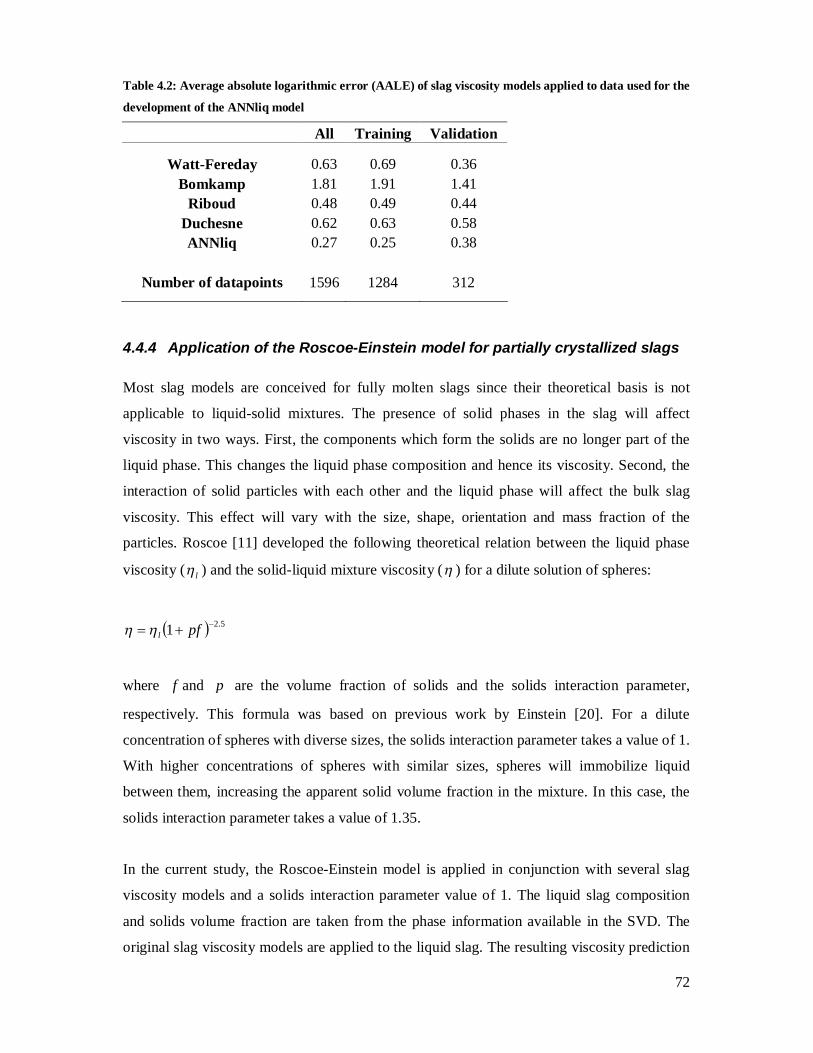
72

Table 4.2: Average absolute logarithmic error (AALE) of slag viscosity models applied to data used for the

development of the ANNliq model

All Training Validation

Watt-Fereday 0.63 0.69 0.36 Bomkamp 1.81 1.91 1.41

Riboud 0.48 0.49 0.44 Duchesne 0.62 0.63 0.58 ANNliq 0.27 0.25 0.38

Number of datapoints 1596 1284 312

4.4.4 Application of the Roscoe-Einstein model for partially crystallized slags

Most slag models are conceived for fully molten slags since their theoretical basis is not

applicable to liquid-solid mixtures. The presence of solid phases in the slag will affect

viscosity in two ways. First, the components which form the solids are no longer part of the

liquid phase. This changes the liquid phase composition and hence its viscosity. Second, the

interaction of solid particles with each other and the liquid phase will affect the bulk slag

viscosity. This effect will vary with the size, shape, orientation and mass fraction of the

particles. Roscoe [11] developed the following theoretical relation between the liquid phase

viscosity ( l ) and the solid-liquid mixture viscosity ( ) for a dilute solution of spheres:

5.21 pfl

where f and p are the volume fraction of solids and the solids interaction parameter,

respectively. This formula was based on previous work by Einstein [20]. For a dilute

concentration of spheres with diverse sizes, the solids interaction parameter takes a value of 1.

With higher concentrations of spheres with similar sizes, spheres will immobilize liquid

between them, increasing the apparent solid volume fraction in the mixture. In this case, the

solids interaction parameter takes a value of 1.35.

In the current study, the Roscoe-Einstein model is applied in conjunction with several slag

viscosity models and a solids interaction parameter value of 1. The liquid slag composition

and solids volume fraction are taken from the phase information available in the SVD. The

original slag viscosity models are applied to the liquid slag. The resulting viscosity prediction

73

is then modified according to the Roscoe-Einstein model. A similar approach was taken by

Kondratiev and Jak [21]. These authors believe the Roscoe-Einstein model is applicable up to

30 vol.% solids. The performance of slag viscosity models with and without the Roscoe-

Einstein modification are compared in Table 4.3. For this comparison, all data in the database

for which phase information is available, and the liquid volume fraction is within 0.70-0.99,

were selected. In total, 637 slag viscosity measurements were selected. Some models which

are available in the SVP were not included in the comparison as they are unable to return a

value for some of the compositions. This was due to a division by zero in one of their

equations. Only three of the nine compared models have improved performance when the

Roscoe-Einstein model is applied. The best accuracy was obtained using the Duchesne model

without the Roscoe-Einstein modification. An AALE of 0.78 is obtained. The second best

accuracy was obtained using the Kalmanovitch-Frank model with the Roscoe-Einstein

modification. An AALE of 0.81 is obtained.

Table 4.3: Average absolute logarithmic error (AALE) of slag viscosity models with and without the

Roscoe-Einstein (RE) modification

Model Without RE With RE

S2 0.81 1.06 Watt-Fereday 1.49 1.93

Bomkamp 2.33 3.14 Shaw 1.00 1.01

Urbain 0.90 0.92 Riboud 0.99 0.88

Kalmanovitch-Frank 0.84 0.81 Duchesne 0.78 0.85 ANNliq 1.31 1.00

4.5 Results and Discussion

In the following, multiple case studies are used to demonstrate how the SVD and SVP can be

applied for specific slag compositions and conditions. The general strategy is to first

determine which slag compositions and conditions are of most interest. The SVD is then used

to identify viscosity data which match or are similar to these slag compositions and

conditions. The SVD will also provide the number of viscosity measurements which match

the selection criteria, and the performance of 24 slag viscosity models with these

74

measurements. Provided there is sufficient data which match the selection criteria, the model

with the best performance is noted. Then, the specific slag compositions and conditions are

entered in the SVP to generate slag viscosity predictions with the best model. Of course if the

exact compositions and conditions of interest are present in the SVD, the measured viscosities

can be directly used instead of relying on models. In addition to providing specific examples

for application of the SVD and SVP, the case studies also demonstrate how confidence in

viscosity data and model performance come into play and the delicate balance between data

selection stringency and data quantity minimums for meaningful analyses. The data selection

criteria for each case study are given in Table 4.4. The number of viscosity measurements

identified and the performance of the slag viscosity models for each case study are given in

Table 4.5.

75

Table 4.4: Selection criteria for each case study (part 1 of 2)

Mass fractions Case Study

Temperature (K)

SiO2 Al2O3 Fe2O3 CaO K2O MgO Na2O SO3 TiO2 P2O5 Other

Min Max Min Max Min Max Min Max Min Max Min Max Min Max Min Max Min Max Min Max Min Max Min Max

1A 0 3000 0.25 0.9 0 0.01 0 0.01 0 0.5 0 0.01 0 0.01 0 0.5 0 0.01 0 0.01 0 0.01 0 0.01 1B 0 3000 0.25 0.9 0 0.01 0 0.01 0 0.5 0 0.01 0 0.01 0 0.5 0 0.01 0 0.01 0 0.01 0 0.01 1C 0 3000 0.25 0.9 0 0.01 0 0.01 0 0.5 0 0.01 0 0.01 0 0.5 0 0.01 0 0.01 0 0.01 0 0.01 1D 0 3000 0.25 0.9 0 0.01 0 0.01 0 0.5 0 0.01 0 0.01 0 0.5 0 0.01 0 0.01 0 0.01 0 0.01 1E 0 3000 0.25 0.9 0 0.01 0 0.01 0 0.5 0 0.01 0 0.01 0 0.5 0 0.01 0 0.01 0 0.01 0 0.01 1F 0 3000 0.25 0.9 0 0.01 0 0.01 0 0.5 0 0.01 0 0.01 0 0.5 0 0.01 0 0.01 0 0.01 0 0.01

2A 0 3000 0.4 0.65 0 0.3 0 0.2 0 0.2 0 0.2 0 0.2 0 0.2 0 1 0 0.01 0 0.01 0 0.01 2B 0 3000 0.2 0.8 0 0.4 0 0.4 0 0.4 0 0.4 0 0.4 0 0.4 0 1 0 0.05 0 0.05 0 0.05 2C 0 3000 0.2 0.8 0 0.4 0 0.4 0 0.4 0 0.4 0 0.4 0 0.4 0 1 0 0.05 0 0.05 0 0.05 2D 0 3000 0.2 0.8 0 0.4 0 0.4 0 0.4 0 0.4 0 0.4 0 0.4 0 1 0 0.05 0 0.05 0 0.05 2E 0 3000 0.2 0.8 0 0.4 0 0.4 0 0.4 0 0.4 0 0.4 0 0.4 0 1 0 0.05 0 0.05 0 0.05

3A 0 3000 0.1 0.6 0 0.3 0 0.03 0.1 0.6 0 0.03 0 0.3 0 0.03 0 1 0 0.03 0 0.03 0 0.03 3B 0 3000 0.1 0.6 0 0.3 0 0.03 0.1 0.6 0 0.03 0 0.3 0 0.03 0 1 0 0.03 0 0.03 0 0.03 3C 0 3000 0.1 0.6 0 0.3 0 0.03 0.1 0.6 0 0.03 0 0.3 0 0.03 0 1 0 0.03 0 0.03 0 0.03 3D 0 3000 0.1 0.6 0 0.3 0 0.03 0.1 0.6 0 0.03 0 0.3 0 0.03 0 1 0 0.03 0 0.03 0 0.03 3E 1793 1913 0.1 0.6 0 0.3 0 0.03 0.1 0.6 0 0.03 0 0.3 0 0.03 0 1 0 0.03 0 0.03 0 0.03 3F 1793 1913 0.1 0.6 0 0.3 0 0.03 0.1 0.6 0 0.03 0 0.3 0 0.03 0 1 0 0.03 0 0.03 0 0.03

75

76

Table 4.4: Selection criteria for each case study (part 2 of 2)

Gas atmosphere volume fractions Case Study

Ar N2 O2 CO2 CO H2 vaccum unknown

Viscosity (Pa·s)

Slag volume fraction

Min Max Min Max Min Max Min Max Min Max Min Max Min Max Min Max Min Max Min Max

Excluded datasets

Exclude data without

phase info?

1A 0 1 0 1 0 1 0 1 0 1 0 1 0 1 0 1 0 1015 0 1 none No 1B 0 1 0 1 0 1 0 1 0 1 0 1 0 1 0 1 0 1015 0.01 1 none Yes 1C 0 1 0 1 0 1 0 1 0 1 0 1 0 1 0 1 0 10 0 1 none No 1D 0 1 0 1 0 1 0 1 0 1 0 1 0 1 0 1 103 106 0 1 none No 1E 0 1 0 1 0 1 0 1 0 1 0 1 0 1 0 1 10 108 0 1 none No 1F 0 1 0 1 0 1 0 1 0 1 0 1 0 1 0 1 108 1015 0 1 none No

2A 0 1 0 1 0 10-7 0 1 0 1 0 1 0 1 0 0 1 100 0 1 none No 2B 0 1 0 1 0 10-7 0 1 0 1 0 1 0 1 0 0 1 100 0.01 1 none Yes 2C 0 1 0 1 0 10-7 0 1 0 1 0 1 0 1 0 0 1 100 0 1 none No 2D 0 1 0 1 0 10-7 0 1 0 1 0 1 0 1 0 0 0 1015 0 1 none No 2E 0 1 0 1 0 10-7 0 1 0 1 0 1 0 1 0 0 100 105 0 1 none No

3A 0 1 0 1 0 1 0 1 0 1 0 1 0 1 0 1 0 1015 0 1 none No 3B 0 1 0 1 0 1 0 1 0 1 0 1 0 1 0 1 0 1015 0.01 1 none Yes 3C 0.01 0.01 0.78 0.78 0.21 0.21 0 0 0 0 0 0 0 0 0 0 0 1015 0 1 none No 3D 0 0.01 0 0.78 0 0.21 0 0 0 0 0 0 0 0 0 1 0 1015 0 1 none No 3E 0 0.01 0 0.78 0 0.21 0 0 0 0 0 0 0 0 0 1 0 1015 0 1 none No 3F 0 0.01 0 0.78 0 0.21 0 0 0 0 0 0 0 0 0 1 0 1015 0 1 Yakushev 1977 No

76

77

Table 4.5: Number of measurements identified and average absolute logarithmic error (AALE) of slag viscosity models for each case study

Model Case Study

1A 1B 1C 1D 1E 1F 2A 2B 2C 2D 2E 3A 3B 3C 3D 3E 3F S2 1.372 1.161 0.761 N/A 2.509 5.109 0.192 0.256 0.266 1.749 0.465 0.694 0.677 0.213 0.772 1.782 0.165

Watt-Fereday 1.675 1.649 0.931 N/A 3.501 4.392 0.250 0.324 0.330 0.931 0.567 0.828 0.842 0.374 0.934 2.112 0.252 Bomkamp 3.763 3.886 3.124 N/A 5.891 3.843 1.579 1.431 1.435 2.072 1.141 1.684 1.718 1.536 1.863 2.346 1.760

Shaw 0.960 0.756 0.775 N/A 0.637 4.736 0.821 0.543 0.553 1.715 0.662 1.033 1.039 0.407 1.145 2.368 0.466 Lakatos 0.584 0.595 0.688 N/A 0.302 0.320 1.183 1.253 1.257 1.659 0.737 2.076 2.137 0.597 2.453 4.525 0.882 Urbain 0.766 0.443 0.253 N/A 1.072 6.523 0.651 0.487 0.490 1.649 0.376 0.591 0.564 0.181 0.636 1.439 0.169 Riboud 0.552 0.217 0.173 N/A 0.249 6.911 0.542 0.526 0.529 1.830 0.325 0.681 0.664 0.084 0.743 1.720 0.128 Streeter 1.735 1.145 0.990 N/A 1.685 12.006 0.618 0.522 0.531 1.526 0.401 0.981 0.969 0.263 1.095 1.580 0.213

Kalmanovitch-Frank 0.743 0.410 0.269 N/A 0.862 6.714 0.424 0.336 0.340 1.654 0.361 0.564 0.535 0.256 0.623 1.496 0.149 BBHLW 0.571 0.321 0.203 N/A 0.717 4.989 0.161 0.285 0.296 1.035 0.575 0.622 0.647 0.194 0.747 1.773 0.196 Duchesne 1.000 0.615 0.610 N/A 0.440 8.503 0.353 0.468 0.454 1.241 0.376 0.949 0.913 0.414 1.041 1.613 0.527 ANNliq 0.620 0.272 0.153 N/A 0.410 7.752 0.311 0.369 0.373 2.332 0.678 0.586 0.552 0.198 0.640 1.521 0.186 S2 +RE N/A 1.170 0.777 N/A 2.524 N/A 0.195 N/A 0.279 N/A 0.418 N/A 0.691 N/A N/A 1.769 0.165

Watt-Fereday +RE N/A 1.680 0.949 N/A 3.514 N/A 0.245 N/A 0.325 N/A 0.522 N/A 0.842 N/A N/A 2.078 0.251 Bomkamp +RE N/A 3.922 3.142 N/A 5.912 N/A 1.622 N/A 1.473 N/A 1.278 N/A 1.775 N/A N/A 2.323 1.761

Shaw +RE N/A 0.794 0.793 N/A 0.677 N/A 0.696 N/A 0.518 N/A 0.586 N/A 1.087 N/A N/A 2.342 0.464 Lakatos +RE N/A 0.629 0.690 N/A 0.336 N/A 1.204 N/A 1.285 N/A 0.749 N/A 1.964 N/A N/A 3.301 0.879 Urbain +RE N/A 0.466 0.269 N/A 1.061 N/A 0.512 N/A 0.446 N/A 0.343 N/A 0.608 N/A N/A 1.421 0.170 Riboud +RE N/A 0.240 0.189 N/A 0.264 N/A 0.421 N/A 0.469 N/A 0.325 N/A 0.679 N/A N/A 1.695 0.130 Streeter +RE N/A 1.162 0.993 N/A 1.724 N/A 0.478 N/A 0.473 N/A 0.384 N/A 0.990 N/A N/A 1.553 0.213

Kalmanovitch-Frank +RE N/A 0.434 0.282 N/A 0.863 N/A 0.316 N/A 0.330 N/A 0.386 N/A 0.555 N/A N/A 1.479 0.150 BBHLW +RE N/A 0.335 0.219 N/A 0.664 N/A 0.191 N/A 0.319 N/A 0.522 N/A 0.685 N/A N/A 1.749 0.195 Duchesne +RE N/A 0.633 0.626 N/A 0.449 N/A 0.396 N/A 0.487 N/A 0.372 N/A 0.987 N/A N/A 1.662 0.526 ANNliq +RE N/A 0.282 0.167 N/A 0.410 N/A 0.293 N/A 0.368 N/A 0.595 N/A 0.571 N/A N/A 1.506 0.186

Number of measurements 167 159 122 0 37 9 57 471 447 807 41 603 558 73 440 98 57

77

78

4.5.1 Case Study 1 – Glass formation

Many glasses are typically composed of SiO2-CaO-Na2O with a few trace elements. The glass

melting process is described by Auchet et al. [22]. A glass viscosity below 10 Pas is required

for refining and homogenizing, between 103 and 106 Pas for blowing and molding, and

around 1012 Pas for annealing [23]. In Case Study 1A, limits on the slag mass fractions were

used to identify measurements with slags which are composed of 25-90 wt.% SiO2, 0-50 wt.%

CaO, 0-50 wt.% Na2O and less than 1 wt% in other components. No limitations were put on

the gas atmosphere composition since the oxidation states of SiO2, CaO and Na2O do not vary

in liquid slag. In all, 167 measurements were identified. With these, the Riboud model is best

(AALE 0.552). However, no results were obtained with the viscosity models applying the RE

modification. This is due to selected measurements with a predicted liquid slag volume

fraction of zero. In Case Study 1B, the measurements with a liquid slag volume fraction of

zero were excluded. The Riboud model is still the best (AALE 0.217). Although the AALE is

now lower, excluding measurements with a predicted liquid slag volume fraction of zero may

remove measurements of interest. It is more important to note that the RE modification does

not improve the model performances. Hence for the next glass formation cases, the limit on

the liquid slag volume fraction was not used. In Case Study 1C, a model is desired

specifically for the refining and homogenization process. Measurements above 10 Pas are

excluded. 122 measurements were identified and the ANNliq model performs best (AALE

0.153). In Case Study 1D, a model is desired specifically for blowing and molding.

Measurements are limited to 103-106 Pas. In this case no data was identified. Therefore, the

viscosity range was increased to 10-108 Pas in Case Study 1E. 37 measurements were

identified and the Riboud model has the best performance (AALE 0.249). Case Study 1F is

focused on the annealing process, with only measurements in the viscosity range 108-1015 Pas

considered. 9 measurements are identified and the Lakatos model has the best performance

(AALE 0.320). It should be noted that the Riboud model has an AALE of 6.911 in this case.

Although the Riboud model has the best general performance for the glass compositions

considered, other models should be applied when considering specific glass formation

processes.

79

4.5.2 Case Study 2 – Entrained flow gasification

A thorough description of entrained flow gasification can be found in [24]. As a heuristic, slag

viscosity should not exceed 25 Pas at the slag tap [9]. In Case Study 2A, mass fraction limits

for the slag composition were specified in the SVD to identify measurements with

compositions similar to typical coal ashes. A maximum volume fraction of 10-7 was specified

for O2 in the gas atmosphere. Measurements with an unknown gas atmosphere were excluded.

Although the fraction of O2 is greater than 10-7 in certain sections of the gasifier, it should be

below this limit near the slag tap in a down-fired gasifier. It is also assumed that the slag in

the gasifier will approach equilibrium with the gas. It is important to specify the gas

atmosphere in this case since the viscosity of slags with high iron content will be significantly

affected due to the multiple possible oxidation states of iron. Furthermore, since the heuristic

limit is at 25 Pas, measurements in the range of 0-100 Pas were specified in the SVD. 57

measurements were identified and the BBHLW model has the best performance (AALE

0.161). In Case Study 2B, the composition limits were expanded to include more

measurements. 471 measurements were identified and the S2 model has the best performance

(AALE 0.256). Depending on the situation, more or less stringent selection criteria may be

preferred, with more or fewer measurements available. The criteria used for Case Study 2B

were kept for the following cases. To determine whether the RE modification can provide

better model performances, measurements with a predicted liquid slag volume fraction of zero

were excluded in Case Study 2C. The results show that the RE modification modestly

worsened the performance of some models, and modestly improved that of others.

Nonetheless, the S2 model still has the best performance (AALE 0.266).

For comprehensive CFD models of entrained flow gasifiers, slag viscosity predictions greater

than 100 Pas are required to model slag flow along the reactor walls, and sometimes to

predict the stickiness of slag particles. In Case Study 2D, the criteria for Case Study 2B were

used, however no limit was placed on viscosity. In this case, the Watt-Fereday model has the

best performance (AALE 0.931). An AALE of 0.931 translates to having predictions which

are on average 8.53 times greater or smaller than the measured value. It may be more useful to

evaluate the performance of models in different viscosity ranges. It was determined in Case

Study 2B that the S2 model should be used in the 0-100 Pas range. It might be assumed that

the slag flow in the gasifier is negligible above 105 Pas, and that the slag is no longer sticky

above this same value. In Case Study 2E, viscosity was limited to the 100-105 Pas range. 41

measurements were identified and the Riboud model has the best performance (AALE 0.325).

80

However, by inspecting the selected measurement data, it should be noted that there are no

measured viscosities greater than 625 Pas. Hence the Riboud model should be applied with

great caution in the 625-105 Pas range.

4.5.3 Case Study 3 – Blast furnace

The importance of slag viscosity in blast furnaces is described by Muller & Erwee [25]. In

Case Study 3A, mass fraction limits for the slag composition were specified in the SVD to

identify measurements with compositions similar to some typical blast furnace slags. 603

measurements are identified and the Kalmanovitch-Frank model has the best performance

with an AALE of 0.564. To determine whether the RE modification can provide better model

performances, measurements with a predicted liquid slag volume fraction of zero were

excluded in Case Study 3B. The results show that the RE modification slightly decreased the

performance of most models. The Kalmanovitch-Frank model still has the best performance

(AALE 0.535). Phase limitations were not applied in the following case studies. Moreover,

the blast furnace gas composition can vary throughout the furnace and with different

operating conditions. In Case Study 3C, it is assumed that an oxidizing gas atmosphere is of

interest. Only measurements performed in air were selected. 73 measurements were identified

and the Riboud model has the best performance (AALE 0.084). However, more

measurements may be desired to provide a better assessment of the models. Many of the

measurements with an unknown gas atmosphere were likely performed in air. Therefore in

Case Study 3D measurements in air or an unknown atmosphere were included. 440

measurements were identified and the Kalmanovitch-Frank model has the best performance

(AALE 0.623). With more data available, other criteria may be specified to approach the

conditions of interest. In Case Study 3E, the temperature range was limited to 1793-1913 K.

98 measurements were identified and the Urbain+RE model has the best performance (AALE

1.421). None of the models seem to have satisfactory performance in this case. Perhaps there

is a specific dataset in the selected measurements which should not be trusted. In Case Study

3F, measurements from Yakushev 1977 were excluded. 57 measurements were identified and

the Riboud model has the best performance (AALE 0.128).

81

4.6 Conclusion

A slag viscosity modeling toolbox, comprised of the SlagViscosityPredictor tool (SVP) and

SlagViscosityDatabase tool (SVD), was developed to facilitate the evaluation and selection of

slag viscosity models for given slag compositions and conditions. The functions of the SVP

and SVD were presented. An artificial neural network for liquid slag viscosity prediction,

ANNliq, was introduced. Furthermore, the Roscoe-Einstein (RE) model was applied in

conjunction with viscosity models and FactSage phase predictions. Glass forming, entrained

flow gasification and blast furnace case studies were presented to demonstrate how the SVD

and SVP can be applied. Slag viscosity model assessment is limited by the quantity and

quality of available slag viscosity measurement data. No one model is applicable to all slag

compositions and conditions, and model performances vary greatly. Model assessment should

be done with great care to balance criteria stringency and the measurement data quantity.

With the case studies, it was found that the RE-modified viscosity models did not have the

best performances. However, this may not be true in other cases. Also, the RE modification

might provide better results with other viscosity models not included in the SVP and SVD, or

with better phase predictions.

There is much room for improvement with the slag viscosity toolbox. More detailed data,

particularly with shear rate provided, should be added to the database. Phase predictions are

expected to improve as well. Certain applications will require much more measurement data

with certain components, such as Cr2O3 and V2O5 for example. In addition, there are more

slag viscosity models available, and some to be developed, which could increase prediction

accuracy. Some of these models can account for non-Newtonian behavior and the effect of

solid particle shapes and sizes. In the effort to improve the toolbox, external contributions are

welcome. More sharing of viscosity data and models in formats which are easy to use is

encouraged.


Part of this research has been funded by the Natural Sciences and Engineering Research

Council of Canada, the Canadian Federal Program for Energy Research and Development

82

(PERD), and the Federal Ministry of Education and Research of Germany in the framework

of Virtuhcon (project number 03Z2FN12).

4.8 References

[1] Richet P. Viscosity and configurational entropy of silicate melts. Geochimica et

Cosmochimica Acta 1984;48:471–83.

[2] Urbain G, Cambier F, Deletter M, Anseau MR. Viscosity of silicate melts. Transactions

& Journal of the British Ceramic Society 1981;80:139–41.

[3] Moriyama R, Takeda S, Onozaki M, Katayama Y, Shiota K, Fukuda T et al. Large-scale

synthesis of artificial zeolite from coal fly ash with a small charge of alkaline solution. Fuel

2005;84:1455–61.

[4] Ledzki A, Migas P, Stachura R, Klimczyk A, Bernasowski M. Dynamic viscosity of

blast furnace primary and final slag with titanium and alkali admixtures. Archives of

Metallurgy and Materials 2009;54:499–509.

[5] Shaw HR. Viscosities of magmatic silicate liquids; an empirical method of prediction.

Am J Sci 1972;272:870–93.

[6] Hurst HJ, Novak F, Patterson JH. Viscosity measurements and empirical predictions for

some model gasifier slags. Fuel 1999;78:439–44.

[7] Verein Deutscher Eisenhüttenleute (Allibert M, Gaye H, Janke D, Keene BJ, Kirner D

et al.). Slag Atlas. 2nd ed. Düsseldorf: Verlag Stahleisen GmbH; 1995.

[8] Vargas S, Frandsen FJ, Dam-Johansen K. Rheological properties of high-temperature

melts of coal ashes and other silicates. Prog. Energy Combust. Sci. 2001;27:237–429.

[9] Browning GJ, Bryant GW, Hurst HJ, Lucas JA, Wall TF. An Empirical Method for the

Prediction of Coal Ash Slag Viscosity. Energy & Fuels 2003;17:731–7.

[10] Duchesne MA, Macchi A, Lu DY, Hughes RW, McCalden D, Anthony EJ. Artificial

neural network model to predict slag viscosity over a broad range of temperatures and slag

compositions. Fuel Processing Technology 2010;91:831–6.

[11] Roscoe R. The viscosity of suspensions of rigid spheres. British Journal of Applied

Physics 1952;3:267–9.

83

[12] Bale CW, Pelton AD, Thompson WT, Eriksson G, Hack K, Chartrand P et al. FactSage:

Thermfact and GTT-Technologies; 2010. Available from http://www.factsage.com/


combustion. Ph. D. thesis, Massachusetts Institute of Technology, United States; 2010.

[14] Lange RA. A revised model for the density and thermal expansivity of K2O-Na2O-CaO-

MgO-Al2O3-SiO2 liquids from 700 to 1900 K: extension to crustal magmatic temperatures.

Contributions to Mineralogy and Petrology 1997;130:1–11.

[15] Jain AK, Mao J, Mohiuddin KM. Artificial neural networks: A tutorial. Computer

1996;29:31–44.

[16] Meireles MRG, Almeida PEM, Simoes MG. A comprehensive review for industrial

applicability of artificial neural networks: Industrial Electronics, IEEE Transactions on.

Industrial Electronics, IEEE Transactions on DOI - 10.1109/TIE.2003.812470 2003;50:585–

601.

[17] Hanao M, Kawamoto M, Tanaka T, Nakamoto M. Evaluation of Viscosity of Mold Flux

by Using Neural Network Computation. ISIJ International 2006;46:346–51.

[18] Saxén H, Zhang X. Neural-network based model of blast furnace slag viscosity.

Proceedings of the International Conference on Engineering Application of Neural Networks

1997;167-70.

[19] The MathWorks, MATLAB, R2008a; 2008.

[20] Einstein A. Eine neue Bestimmung der Moleküldimensionen. Annalen der Physik

1906;324:289–306.

[21] Kondratiev A, Jak E. Predicting coal ash slag flow characteristics (viscosity model for

the Al2O3-CaO-`FeO'-SiO2 system). Fuel 2001;80:1989–2000.

[22] Auchet O, Riedinger P, Malasse O, Iung C. First-principles simplified modelling of

glass furnaces combustion chambers. Control Engineering Practice 2008;16:1443–56.

[23] Le Bourhis E. Glass: Mechanics and Technology. 1st ed. Weinheim: WILEY-

VCHVerlag; 2007.

[24] Higman C, van der Burgt M. Gasification Processes. In: Gasification (Second Edition).

Burlington: Gulf Professional Publishing; 2008, p. 91–191.

84

[25] Muller J, Erwee M. Blast Furnace Control using Slag Viscosities and Liquidus

Temperatures with Phase Equilibria Calculations. Southern African Pyrometallurgy 2011,

Southern African Institute of Mining and Metallurgy, Johannesburg, 6-9 March 2011; 309-26.

85

Chapter 5. Flow behaviour of slags from coal and petroleum coke blends Published in Fuel (2012) 97, p. 321-328

Marc A. Duchesnea, Alexander Y. Ilyushechkinb, Robin W. Hughesc, Dennis

Y. Luc, David J. McCaldenc, Arturo Macchia, Edward J. Anthonyc



bCSIRO Energy Technology, Queensland Centre for Advanced Technologies, 1

Technology Court, Pullenvale QLD 4069, Australia


86

5.1 Abstract

Petroleum coke may be used as a fuel for entrained-flow slagging gasification. It may be

blended with coal to provide a more attractive feedstock. The coal provides the benefits

of enhancing reactivity and increasing the amount of slag coating the gasifier walls, while

the petroleum coke increases the heating value of the fuel blend. The slagging behavior of

the petroleum coke or blend must be known to determine if it is a suitable feedstock. In

the present study, the slag viscosities of coal, petroleum coke and coal/petroleum coke

blends were measured in the temperature range of 1175-1650ºC. Two different viscosity

measurement apparatuses were used in separate laboratories. Some viscosity

measurements were repeated to test reproducibility of the results. Also, slags with and

without sulphur were tested to determine whether the effect of sulphur can be neglected.

The largest deviation between repeated log(viscosity in Pas) measurements is 0.11. Both

petroleum coke slags tested are suitable for operation at or above 1275°C. The

temperature range of operability for one coal slag tested increased when blended with

petroleum coke ash, but did not significantly change for other coal slags tested. Some

effects of blending on viscosity behaviour can be explained by network former and

modifier theory. Other effects are attributed to solids formation which was investigated

via slag quenching experiments and FactSage predictions. Below 1300°C, vanadium, a

major component of petroleum coke ashes, promotes the formation of spinel which

increases slag viscosity.

Keywords: Slag, Viscosity, Coal, Petroleum coke, Gasification

87

5.2 Introduction

Production of petroleum coke, a by-product of the oil refining industry, has been and is

expected to continue to increase [1]. The major factors driving this increase include the

rising demand for transport fuels, the use of heavier crude oils and new environmental

regulations pushing for reduced waste and highly refined fuels. Due to petroleum coke’s

high heating value and low cost, there is much interest in its use as a primary fuel or in

coal-petroleum coke blends. Although various technologies can utilize petroleum coke as

a fuel for power generation, gasification can provide lower gaseous emissions and less

solid waste [2]. Another advantage of gasification for petroleum coke conversion is the

encapsulation of hazardous metals such as vanadium and nickel in non-leachable slag.

Furthermore, gasification may be used to provide steam and hydrogen in addition to

power generation. This can be beneficial when the gasifier is sited near the petroleum

coke-producing oil refinery which requires steam, hydrogen and power [3].

The majority of the successful high throughput coal gasifiers developed in the past 60

years are of the entrained-flow slagging type [4]. In this type of gasifier, most of the

inorganic component of the fuel (ash) is partially or fully melted, sticks to the reactor

wall and flows to the bottom as slag. To determine the performance and profitability of a

slagging gasifier it is important to know the slagging properties of the intended fuel. A

slag which is too viscous may accumulate on the reactor wall until the reactor begins to

plug, requiring corrective action which may include increasing the gasifier operating

temperature, oxygen injection at the slag tap, or ceasing operation. As a rule of thumb,

slag viscosity should not exceed 25 Pas at the slag tapping temperature [5,6]. If a fuel’s

slag is too viscous, the gasifier operating temperature may be increased, a fluxing agent

such as limestone or dolomite may be added, and/or the fuel may be blended with another

fuel. Blending fuels may also be necessary if there are issues with fuel availability, flame

stability or ash content.

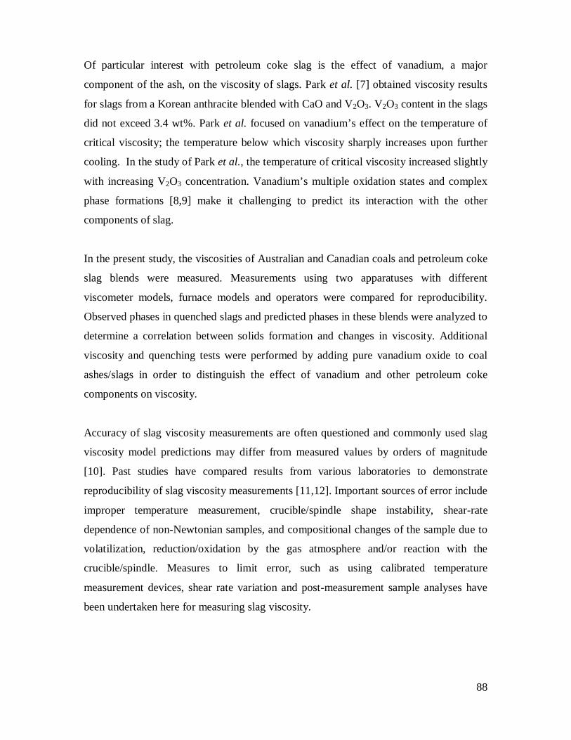
88

Of particular interest with petroleum coke slag is the effect of vanadium, a major

component of the ash, on the viscosity of slags. Park et al. [7] obtained viscosity results

for slags from a Korean anthracite blended with CaO and V2O3. V2O3 content in the slags

did not exceed 3.4 wt%. Park et al. focused on vanadium’s effect on the temperature of

critical viscosity; the temperature below which viscosity sharply increases upon further

cooling. In the study of Park et al., the temperature of critical viscosity increased slightly

with increasing V2O3 concentration. Vanadium’s multiple oxidation states and complex

phase formations [8,9] make it challenging to predict its interaction with the other

components of slag.

In the present study, the viscosities of Australian and Canadian coals and petroleum coke

slag blends were measured. Measurements using two apparatuses with different

viscometer models, furnace models and operators were compared for reproducibility.

Observed phases in quenched slags and predicted phases in these blends were analyzed to

determine a correlation between solids formation and changes in viscosity. Additional

viscosity and quenching tests were performed by adding pure vanadium oxide to coal

ashes/slags in order to distinguish the effect of vanadium and other petroleum coke

components on viscosity.

Accuracy of slag viscosity measurements are often questioned and commonly used slag

viscosity model predictions may differ from measured values by orders of magnitude

[10]. Past studies have compared results from various laboratories to demonstrate

reproducibility of slag viscosity measurements [11,12]. Important sources of error include

improper temperature measurement, crucible/spindle shape instability, shear-rate

dependence of non-Newtonian samples, and compositional changes of the sample due to

volatilization, reduction/oxidation by the gas atmosphere and/or reaction with the

crucible/spindle. Measures to limit error, such as using calibrated temperature

measurement devices, shear rate variation and post-measurement sample analyses have

been undertaken here for measuring slag viscosity.

89

5.3 Experimental

5.3.1 Coal and petroleum coke selection

Several coal and petroleum coke ashes, slags, and representative synthetic oxide mixtures

were used in this study. Compositions are given in Table 5.1. The listed compositions

exclude some components which represent less than 1 wt.% of the ash and were

normalized to 100%. Artificial coal ashes were prepared by mixing laboratory or

analytical grade Al2O3, CaO, Fe2O3, K2CO3, MgO, Na2CO3, NiO, S, SiO2, TiO2 and V2O5

powders. Real coal and petroleum coke ashes were prepared by ashing of the coal or

petroleum coke at 700-750 °C for 20-30 h. Slags S1 and S2 were collected from Siemens’

pilot plant gasifier in Germany. Slags S3 and S4 were collected from CanmetENERGY’s

pilot plant gasifier in Canada.

Table 5.1: Composition of coal and petcoke ashes/slags

Weight% Oxide

P1a P1b P2 C1a C1b S1 S2 S3 S4 SiO2 37.77 40.66 43.41 58.02 60.01 49.62 47.73 49.24 46.54 Al2O3 16.60 17.87 14.82 23.47 24.27 18.22 24.07 21.02 21.29 Fe2O3 7.35 7.91 9.41 4.55 4.71 24.36 15.41 7.38 12.21 TiO2 1.10 1.19 0.62 0.53 0.54 1.17 1.49 0.68 1.02 CaO 15.82 17.03 4.13 5.63 5.82 3.27 8.25 13.15 10.34 MgO 3.87 4.17 1.36 1.57 1.62 1.62 0.97 2.85 2.47 Na2O 1.67 1.80 1.13 2.34 2.42 0.55 0.28 2.71 1.43 K2O 0.96 1.03 1.75 0.58 0.60 0.45 0.30 0.82 0.67 V2O5 6.67 7.18 20.69 <1 0.01 <1 <1 <1 <1 NiO 1.09 1.17 2.68 <1 <1 <1 <1 <1 0.61 Cr2O3 <1 <1 <1 <1 <1 <1 <1 2.15 3.43 P2O5 <1 <1 <1 <1 <1 0.73 1.49 <1 <1 SO3 7.11 <1 <1 3.32 <1 <1 <1 <1 <1

90

P1a is real ash produced from an Alberta, Canada oil sands delayed coke. P1b is an

artificial ash based on the composition of P1a, excluding sulphur. P2 is an artificial ash

based on the ash composition of petroleum coke sourced from an eastern Canadian power

utility, excluding sulphur. C1a is an artificial ash based on the ash composition of an

Alberta, Canada sub-bituminous coal. C1b is the equivalent of C1a without sulphur. S1 is

slag produced from gasification of a sub-bituminous coal from Western Australia,

Australia. S2 is slag produced from gasification of a high volatile bituminous coal from

New South Wales, Australia. S3 is slag produced from the gasification of a sub-

bituminous coal from Alberta, Canada. S4 is slag produced from the gasification of a

50/50 blend of S3 and P2’s parent fuels.

Although S4 is from a 50/50 blend of S3 and P2’s parent fuels, its composition can not be

calculated based on the compositions of S3 and P2. Based on the compositions of S3 and

P2, S4 is expected to contain several weight percent V2O5. However, S4 does not contain

an appreciable amount of V2O5. It is believed that due to lower reactivity, the petroleum

coke ash reported to the fly ash stream rather than the coarse slag. Also, S3 and S4 have

higher Al2O3 and Cr2O3 than the ash of their parent fuels. These components are believed

to have been taken up by the slag from the gasifier refractory. Future testing will be done

to study enrichment and depletion in the gasifier of various slag components.

The base coal and petroleum coke ashes/slags, as described above, were blended for

viscosity measurements and quenching experiments. For sample identification in this

paper, the identifier of the majority ash is listed first, followed by the wt.% (relative to the

majority ash) and identifer of the secondary ash. For example, C1b+25P1b contains 25 g

of P1b for every 100 g of C1b.

5.3.2 Viscosity measurements

Slag viscosity measurements at CSIRO, Australia, were performed using a Haake high

temperature viscometer using a rotational bob [13]. Ashes were placed in a molybdenum

crucible and heated to 1200 ºC and left to equilibrate overnight. They were then heated to

1520-1550 ºC in a nitrogen atmosphere. Sample temperature was measured with a

91

thermocouple placed near the sample location. The crucible was placed in a sacrificial

graphite sleeve to consume free oxygen in the constant nitrogen gas flow. Oxygen partial

pressure (pO2) in the system has been measured using an oxygen probe (HT oxygen

probe, Australian Oxytrol Systems). At temperatures between 1200-1450 ºC, pO2 values

near the slag surface were between 2.8x10-6 and 2.9x10-4 Pa, confirming the reducing

nature of the experimental conditions. Viscosity measurements were performed using a

molybdenum rotating bob connected to a viscometer head. Measurements were

conducted at incremental temperature reduction steps within the temperature range 1200-

1550 ºC. The cooling step for each set of measurements was of 25 ºC with at least 30 min

intervals to equilibrate temperatures and compositions inside the crucible. At each step,

shear stress is measured with varying shear rate to detect non-Newtonian behaviour, and

the slag viscosity was measured several times to ensure the repeatability of

measurements. The average of these measurements was used as the value of viscosity

[14].

Slag viscosity measurements at CanmetENERGY, Canada, were performed in a Carbolite

3 litre BLF1700 furnace with a Brookfield RVDV-IIIU rheometer. Both are connected to

a PC for external control. Unless otherwise indicated, samples are placed in a

molybdenum crucible. The crucible is placed in a custom-built alumina chamber within

the furnace for gas atmosphere control and spill protection. A type B thermocouple is

inserted into the chamber to monitor the sample temperature. Argon is fed at 0.4 dm3/min

and a graphite sleeve is placed around the molybdenum crucible to consume trace

oxygen. Mössbauer spectroscopy of a slag sample after viscosity measurements indicates

that all iron atoms are in the ferrous state, confirming the reducing nature of the

experimental conditions. A molybdenum spindle, attached to the rheometer, reaches the

slag sample and is rotated to measure torque. The operation of the rheometer was

validated with the National Institute of Standards and Technology's (NIST, United States)

standard reference material 717a. Ash samples were first heated to 1225 ºC and left

overnight for equilibration. They were then heated to 1475-1650 °C. Measurements were

conducted at incremental temperature reduction steps within the temperature range 1175-

1650 ºC. The cooling step for each set of measurements was of 25 ºC with at least 25 min

intervals to equilibrate temperatures and compositions inside the crucible. At each

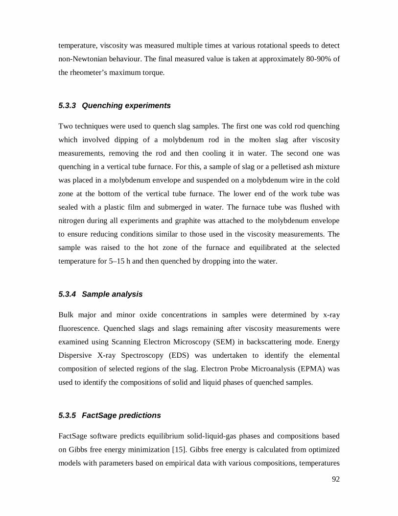
92

temperature, viscosity was measured multiple times at various rotational speeds to detect

non-Newtonian behaviour. The final measured value is taken at approximately 80-90% of

the rheometer’s maximum torque.

5.3.3 Quenching experiments

Two techniques were used to quench slag samples. The first one was cold rod quenching

which involved dipping of a molybdenum rod in the molten slag after viscosity

measurements, removing the rod and then cooling it in water. The second one was

quenching in a vertical tube furnace. For this, a sample of slag or a pelletised ash mixture

was placed in a molybdenum envelope and suspended on a molybdenum wire in the cold

zone at the bottom of the vertical tube furnace. The lower end of the work tube was

sealed with a plastic film and submerged in water. The furnace tube was flushed with

nitrogen during all experiments and graphite was attached to the molybdenum envelope

to ensure reducing conditions similar to those used in the viscosity measurements. The

sample was raised to the hot zone of the furnace and equilibrated at the selected

temperature for 5–15 h and then quenched by dropping into the water.

5.3.4 Sample analysis

Bulk major and minor oxide concentrations in samples were determined by x-ray

fluorescence. Quenched slags and slags remaining after viscosity measurements were

examined using Scanning Electron Microscopy (SEM) in backscattering mode. Energy

Dispersive X-ray Spectroscopy (EDS) was undertaken to identify the elemental

composition of selected regions of the slag. Electron Probe Microanalysis (EPMA) was

used to identify the compositions of solid and liquid phases of quenched samples.

5.3.5 FactSage predictions

FactSage software predicts equilibrium solid-liquid-gas phases and compositions based

on Gibbs free energy minimization [15]. Gibbs free energy is calculated from optimized

models with parameters based on empirical data with various compositions, temperatures

93

and pressures. This information is contained within compound and solution databases

which must be carefully selected prior to equilibrium calculations. The FactSage 6.2

Equilib module was utilized with the FACT53 and FToxid databases. 1 g of N2 per 100 g

of sample was included in the calculations. Some oxide components representing less

than 1 wt.% of the samples were excluded. Of all gas compounds, solid compounds and

solutions which can be formed, only solutions containing titanium were excluded. These

components and solutions were excluded as to not exceed the maximum phase limits in

FactSage.

5.4 Results

5.4.1 Validation of viscosity measurements

Viscosity values are given as logarithmic (base 10) values, with viscosity in Pas. This

makes it easier to view trends in temperature-viscosity curves since a large range of

viscosity is covered and the logarithm viscosity, herein referred to as LV, is roughly a

linear function of temperature. Furthermore, differences between LVs can be interpreted

as a factor difference between viscosities. For example, LVs with a difference of 0.2

correspond to viscosities with a factor difference of 1.58 (i.e., 100.2).

Various temperature-LV curves were generated to test the repeatability of results with the

CanmetENERGY viscosity measuring apparatus, and the reproducibility of results

between the CanmetENERGY and CSIRO viscosity apparatuses (Figure 5.1). Two

temperature-LV curves were generated four months apart for C1b as a measure of

repeatability with the CanmetENERGY viscosity equipment. Over the temperature range

of 1400-1550 °C, and the LV range of 1.62-2.48, the greatest deviation in LV is 0.09.

Reproducibility between the CanmetENERGY and CSIRO viscosity rigs was determined

by measuring the viscosity of S3 with both. Over the temperature range of 1300-1475 °C,

and the logarithmic viscosity range of 1.09-2.14, the greatest deviation in LV is 0.04. A

few viscosity measurements were conducted to determine whether sulphur can be

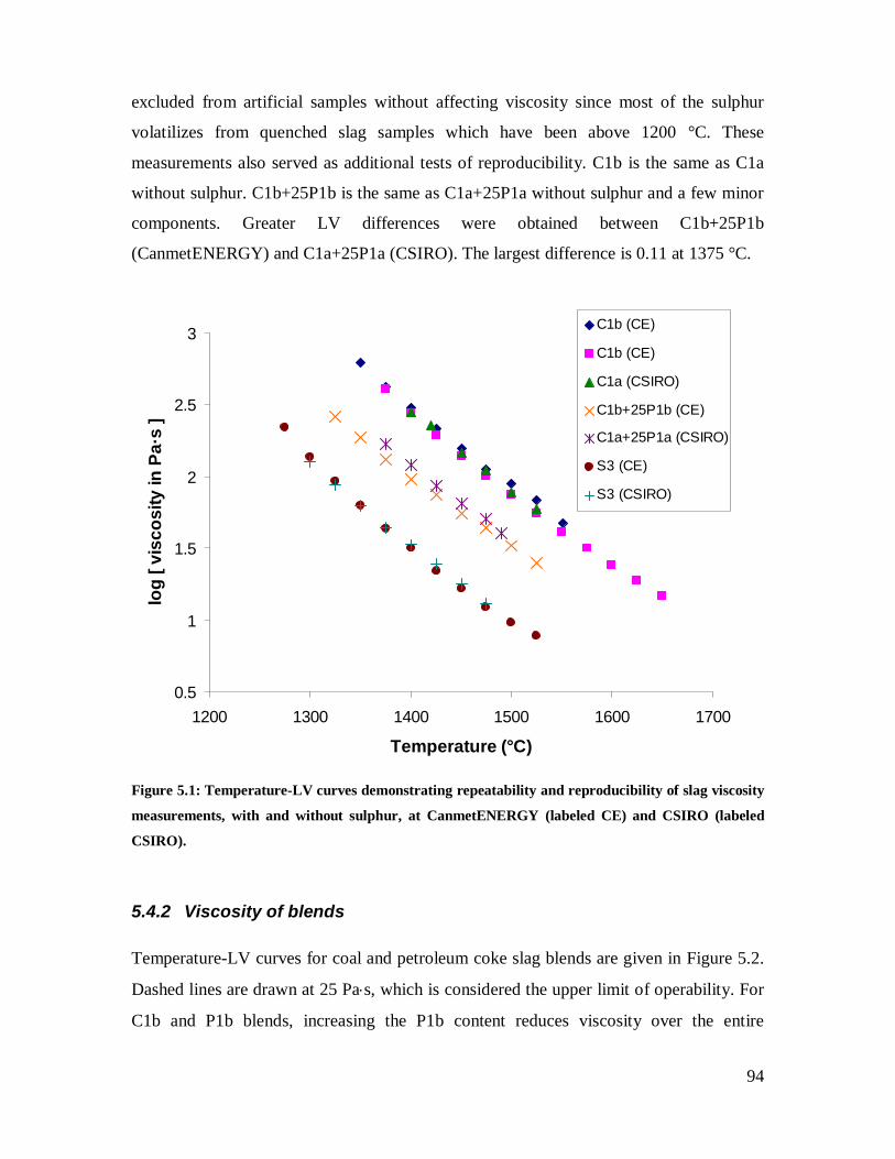
94

excluded from artificial samples without affecting viscosity since most of the sulphur

volatilizes from quenched slag samples which have been above 1200 °C. These

measurements also served as additional tests of reproducibility. C1b is the same as C1a

without sulphur. C1b+25P1b is the same as C1a+25P1a without sulphur and a few minor

components. Greater LV differences were obtained between C1b+25P1b

(CanmetENERGY) and C1a+25P1a (CSIRO). The largest difference is 0.11 at 1375 °C.

0.5

1

1.5

2

2.5

3

1200 1300 1400 1500 1600 1700

Temperature (°C)

log

[ vis

cosi

ty in

Pa·

s ]

C1b (CE)

C1b (CE)

C1a (CSIRO)

C1b+25P1b (CE)

C1a+25P1a (CSIRO)

S3 (CE)

S3 (CSIRO)

Figure 5.1: Temperature-LV curves demonstrating repeatability and reproducibility of slag viscosity

measurements, with and without sulphur, at CanmetENERGY (labeled CE) and CSIRO (labeled

CSIRO).

5.4.2 Viscosity of blends

Temperature-LV curves for coal and petroleum coke slag blends are given in Figure 5.2.

Dashed lines are drawn at 25 Pas, which is considered the upper limit of operability. For

C1b and P1b blends, increasing the P1b content reduces viscosity over the entire

95

temperature range tested, with pure P1b having the lowest viscosity. C1b has a viscosity

above 25 Pas for the entire temperature range tested, while C1b+100P1b is suitable for

operation above 1400 °C. S1 and its blends all cross the 25 Pas line between 1270 and

1290 °C. At 1450 °C, S1+P1a blends have LV’s which are up to 0.16 lower than the LV

of S1. At 1200 °C, S1+P1a blends have LV’s which are up to 0.21 higher than the LV of

S1. Viscosity of pure P1b, assumed to be the same as P1a, is lower over the entire

temperature range tested, albeit with a sharper increase in viscosity upon cooling. S2 and

its blends all cross the 25 Pas line between 1310 and 1340 °C. At 1475 °C, S2+50P1a

has an LV which is 0.08 lower than the LV of S2. At 1250 °C, S1+50P1a has an LV

which is 0.07 higher than the LV of S2. Viscosity of pure P1b is lower over the entire

temperature range tested, albeit with a sharper increase in viscosity upon cooling. When

S2 was mixed with 2.2 wt% V2O5, which is the same amount of V2O5 as in S2+50P1a,

the LV was higher than S2’s LV by 0.04 at 1450 °C, and by 0.21 at 1300 °C. Both S3 and

S4 have a viscosity below 25 Pas at temperatures above 1400 ºC. S4 has a lower

viscosity than S3 at temperatures above 1400 ºC, and a higher viscosity at temperatures

below 1400 ºC. Adding 5 wt% V2O5 to S3 reduces the LV by 0.28 at 1525 ºC, but

increases the LV by 0.17 at 1300 ºC. P2, based on the petroleum coke which had been

used to produce S4, has a viscosity below 25 Pas over the entire temperature range

tested. Note that the viscosity of P2 was measured with an alumina crucible and spindle.

An attempt had been made to measure its viscosity with a molybdenum crucible and

spindle; however, the viscosity did not stabilize after 4 hours at 1475 ºC.

96

Figure 5.2: Temperature-LV curves of coal and petcoke slag blends. Dashed lines are drawn at 25

Pa·s. (part 1 of 2)

-0.5

0

0.5

1

1.5

2

2.5

3

1175 1225 1275 1325 1375 1425 1475 1525 1575Temperature (°C)

log

[ vis

cosi

ty in

Pa·

s ]

C1bC1b+25P1bC1b+50P1bC1b+100P1bP1b

-0.5

0

0.5

1

1.5

2

2.5

3

1175 1225 1275 1325 1375 1425 1475 1525 1575Temperature (°C)

log

[ vis

cosi

ty in

Pa·

s ]

S1

S1+25P1a

S1+50P1a

P1b

97

Figure 5.2: Temperature-LV curves of coal and petcoke slag blends. Dashed lines are drawn at 25

Pa·s. (part 2 of 2)

-0.5

0

0.5

1

1.5

2

2.5

3

1175 1225 1275 1325 1375 1425 1475 1525 1575Temperature (°C)

log

[ vis

cosi

ty in

Pa·

s ]

S3

S4

P2

S3+5V2O5

-0.5

0

0.5

1

1.5

2

2.5

3

1175 1225 1275 1325 1375 1425 1475 1525 1575Temperature (°C)

log

[ vis

cosi

ty in

Pa·

s ]

S2

S2+50P1a

P1b

S2+2.2V2O5

98

5.4.3 Slag microstructure

In order to understand the viscosity behaviour of investigated slags below the liquidus

temperature, a series of slag quenching experiments was conducted. Quenching

temperatures were selected near the lower temperature limit of the viscosity

measurements. Figure 5.3 shows micrographs of the C1b and C1b+xP1b slags quenched

from 1350 °C and 1300 °C. At 1350 °C, only C1b slag contains solids. These are

identified by EPMA as mullite. Both blended samples have only a liquid phase at this

temperature. At 1300 °C, C1b slag still has more solids than C1b+xP1b blends. In the

blends, vanadium-rich spinels are present. It is clear that for C1b coal ash, blending with

petroleum coke ash significantly changes phase equilibria in the slag system and lowers

the liquidus temperature. Figure 5.4 shows micrographs of the S1 and S1+xP1a slags

quenched from 1200 °C. S1 slag is fully liquid, while S1+25P1a and S1+50P1a blends

have spinel and spinel with feldspar, respectively. Figure 5.5 shows micrographs of the

S2, S2+50P1a and S2+2.2V2O5 slags quenched from 1250 °C. The pure S2 slag has only

a small amount of mullite. For S2+50P1a slag, the composition shifts to the spinel

primary phase field. For S2 mixed with 2.2 wt% V2O5, which is the same amount of

V2O5 as in S2+50P1a, feldspar and vanadium-rich spinel are present. Figure 5.6 shows

micrographs of the S3, S4 and S3+5V2O5 slags quenched from 1325 °C and 1275 °C. At

1325 °C, S3 has chromium-rich spinel and feldspar, while S4 has chromium-rich spinel

containing a small amount of vanadium oxide (~ 2 wt.%). At 1275 °C, both S3 and S4

have chromium–rich spinel and a significant amount of feldspar. The chromium–rich

spinel in S4 also contains some (~2 wt.%) vanadium oxide. For S3 mixed with 5 wt.%

V2O5, which is in the same proportion as for the parent fuels of S4, chromium-vanadium

spinel is present at 1325 °C. At 1275 °C, feldspar appears as a second solid phase. The

quenched S3+5V2O5 samples are very similar to the quenched S4 samples.

99

Figure 5.3: Microstructure of slags quenched from 1350 °C: C1b (a), C1b+50P1b (b), C1b+100P1b

(c); and quenched from 1300 °C: C1b (d), C1b+50P1b (e), C1b+100P1b (f). Legend: Liq- former

liquid phase, Mul- mullite, Spi- spinel.

Figure 5.4: Microstructure of slags quenched from 1200 °C: S1 (a), S1+25P1a (b), S1+50P1a (c).

Legend: Liq- former liquid phase, Fel- feldspar, Spi- spinel.

Figure 5.5: Microstructure of slags quenched from 1250 °C: S2 (a), S2+50P1 (b), S2+2.2V2O5 (c).

Legend: Liq- former liquid phase, Fel- feldspar, Mul- mullite, Spi- spinel.

100

Figure 5.6: Microstructure of slags quenched from 1325 °C: S3 (a), S4 (b), S3+5V2O5 (c); and

quenched from 1275 °C: S3 (d), S4 (e), S3+5V2O5 (f). Legend: Liq- former liquid phase, Fel-

feldspar, Spi- spinel.

The mass fractions of solids in the coal and petroleum coke slag blends, as predicted by

FactSage, are given in Figure 5.7. The amount and type of solids predicted (type data not

shown) generally do not match with results from quenching experiments. For instance,

below 1300 °C, the FactSage predicted solids fractions are above 20% for most samples

tested. Also, since vanadium is only included as solid compounds and not as slag solution

species in the FactSage databases, all vanadium is predicted to be in solid form for the

entire temperature range of all samples which contain vanadium.

101

Figure 5.7: Predicted solids mass fractions of coal and petcoke slag blends using FactSage. (part 1 of

2)

0

0.1

0.2

0.3

0.4

0.5

0.6

0.7

0.8

0.9

1

1175 1225 1275 1325 1375 1425 1475 1525 1575

Temperature (°C)

Sol

ids

fract

ion

C1bC1b+25P1bC1b+50P1bC1b+100P1bP1b

0

0.1

0.2

0.3

0.4

0.5

0.6

0.7

0.8

0.9

1

1175 1225 1275 1325 1375 1425 1475 1525 1575

Temperature (°C)

Solid

s fra

ctio

n

S1S1+25P1aS1+50P1aP1b

102

Figure 5.7: Predicted solids mass fractions of coal and petcoke slag blends using FactSage. (part 2 of

2)

0

0.1

0.2

0.3

0.4

0.5

0.6

0.7

0.8

0.9

1

1175 1225 1275 1325 1375 1425 1475 1525 1575

Temperature (°C)

Solid

s fra

ctio

nS2S2+50P1aP1bS2+2.2V2O5

0

0.1

0.2

0.3

0.4

0.5

0.6

0.7

0.8

0.9

1

1175 1225 1275 1325 1375 1425 1475 1525 1575

Temperature (°C)

Sol

ids

fract

ion

S3S4P2S3+5V2O5

103

5.4.4 Reactivity with crucible and spindle

Post-run analysis of the slags indicates that MoO3 content does not exceed 1 wt.% for

slags containing <5 wt.% V2O5. For these slags, 10-15% of the V2O5 in the slag is lost by

reaction with the molybdenum crucible. Changes in composition are greater for slags

with ≥5 wt.% V2O5. Figure 5.8 shows microstructures of P2 after viscosity tests

conducted in both molybdenum and alumina crucibles. Slag-crucible reaction products,

indicated by arrows, are observed at the slag-crucible interface. EPMA analysis reveals

that the reaction products are vanadium-molybdenum metal and vanadium-containing

spinel for the viscosity measurements carried out in molybdenum and alumina crucibles,

respectively. Table 5.2 shows bulk compositions of vanadium-rich slags before and after

viscosity measurements. For slags processed in molybdenum crucibles, the V2O5 content

decreases by 3-10 percentage points by mass during viscosity tests. This is equivalent to a

loss of up to 66% of the initial V2O5 content. MoO3 content is increased by up to 10 wt%.

Compositional changes of P2 processed in an alumina crucible include a loss of 50% of

the initial V2O5 content, and an increase by 6 wt.% of the Al2O3 content.

Figure 5.8: Microstructure of slags in Mo (a) and alumina (b) crucibles.

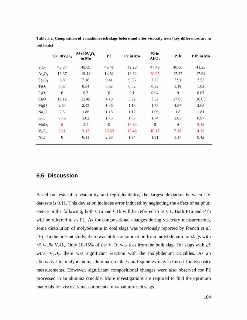
104

Table 5.2: Composition of vanadium-rich slags before and after viscosity tests (key differences are in

red fonts)

S3+10V2O5 S3+10V2O5

in Mo P2 P2 in Mo P2 in Al2O3

P1b P1b in Mo

SiO2 45.37 48.69 43.41 42.28 47.49 40.66 41.25 Al2O3 19.37 19.14 14.82 13.82 20.05 17.87 17.94 Fe2O3 6.8 7.18 9.41 9.56 7.23 7.91 7.53 TiO2 0.63 0.54 0.62 0.52 0.32 1.19 1.03 P2O5 0 0.5 0 0.1 0.04 0 0.05 CaO 12.12 12.48 4.13 3.72 3.52 17.03 16.03 MgO 2.63 2.43 1.36 1.13 1.73 4.87 3.65 Na2O 2.5 1.86 1.13 1.12 1.06 1.8 1.81 K2O 0.76 1.02 1.75 1.67 1.74 1.03 0.97 MoO3 0 2.3 0 10.64 0 0 5.16 V2O5 9.21 3.13 20.69 13.46 10.17 7.18 4.13 NiO 0 0.11 2.68 1.94 1.91 1.17 0.42

5.5 Discussion

Based on tests of repeatability and reproducibility, the largest deviation between LV

datasets is 0.11. This deviation includes error induced by neglecting the effect of sulphur.

Hence in the following, both C1a and C1b will be referred to as C1. Both P1a and P1b

will be referred to as P1. As for compositional changes during viscosity measurements,

some dissolution of molybdenum in coal slags was previously reported by French et al.

[16]. In the present study, there was little contamination from molybdenum for slags with

<5 wt.% V2O5. Only 10-15% of the V2O5 was lost from the bulk slag. For slags with ≥5

wt.% V2O5, there was significant reaction with the molybdenum crucibles. As an

alternative to molybdenum, alumina crucibles and spindles may be used for viscosity

measurements. However, significant compositional changes were also observed for P2

processed in an alumina crucible. More investigations are required to find the optimum

materials for viscosity measurements of vanadium-rich slags.

105

Differences in slag viscosities can be related to the slag compositions. Liquid slag

components can be classified into three categories; network formers, network modifiers

and amphoterics [10]. Network formers (e.g., Si) increase viscosity. Network modifiers

(e.g., Na, K, Mg, Ca) decrease viscosity. Amphoterics (e.g., Al, Fe) can act either as

network formers or modifiers. Other components have not been as thoroughly studied

and are harder to classify (e.g., Ti, V, Ni, Cr). A previous study produced viscosity data

for blends of C1, P1, limestone and/or dolomite [17]. It was shown that both limestone

and dolomite are effective for reducing the viscosity of C1 and C1/P1 slags. The addition

of 25 wt.% P1 also reduces the viscosity of C1, but not to the same extent as adding 25

wt.% limestone or dolomite. In the current study, the effect of adding petroleum coke ash

to C1, S1, S2 and S3 was investigated. Based on the network former and modifier

contents, adding P1 to C1, S1 and S2 should decrease their viscosity. Also, S4 should

have a lower viscosity than S3. From the results, adding P1 to C1 decreases viscosity

over the entire temperature range tested. Adding P1 to S1 and S2 only decreases the

viscosity at certain temperatures. S4’s viscosity is only lower than S3’s viscosity above

1375°C. The effect of amphoterics and unclassified components may be causing the

viscosity to increase. Another factor which causes viscosity to increase is the presence

solids.

Based on quenched sample analyses, addition of P1 to C1 reduced the liquidus

temperature which, in addition to the network former and modifier contents, contributed

to the lower viscosities of the C1+xP1 blends compared to C1. Adding P1 to S1 increased

the liquidus temperature, which led to an increase in viscosity below 1275 °C. For S2,

S2+50P1 and S2+2.2V2O5, a difference in liquidus temperature was not detected by

quenching experiments. This is also true for S3, S4 and S3+5V2O5. However, more

quenching experiments may reveal a difference in liquidus temperature. For all slags

which contain vanadium, spinel is present in slags quenched at or below 1300 °C. This is

likely associated to the sharper increase in viscosity upon cooling of these slags,

compared to the slags which do not contain vanadium. FactSage results are ambiguous

since the solid fraction curves are similar and crossover multiple times, particularly if one

106

does not consider vanadium solids at higher temperatures. Also, FactSage predictions

have very high solids fractions for most slags below 1300 °C. Given the quenched sample

observations, this has been shown not to occur.

C1 has a very high viscosity that makes its parent fuel a poor candidate as a feedstock for

slagging gasification. Adding P1 to C1 reduced the slag viscosity to below 25 Pas over

part of the temperature range tested. When P1 is added to S1 or S2, the temperature at

which the slag viscosity reaches 25 Pas varies by less than 30 °C. S3 and S4 both cross

the 25 Pas threshold at nearly the same temperature. At and above 1275 °C, both P1 and

P2 are below 25 Pas.

5.6 Conclusion

Repeatability and reproducibility of slag viscosity measurements are demonstrated.

Comparing slags with and without sulphur, the largest deviation of LV measurements

obtained with different apparatuses is 0.11. A series of viscosity measurements and

microstructural analyses of quenched samples indicate that blending coal ashes with

petroleum coke ash has a complex effect on the viscosity. Adding petroleum coke ash to

coal ashes changes the relative amounts of network formers and modifiers, as well as the

liquidus temperature and types/quantity of solids in the resulting slags. Vanadium, a

major component of petroleum coke ashes, has the particular effect of promoting the

formation of spinel in slags below 1300 °C. These combined effects lead to an increased

temperature range of operability for one coal ash tested, but do not significantly change

the range of operability for the other coal ashes tested. Both petroleum coke ashes tested

are suitable for operation at or above 1275 °C when they are not blended with coal ash.

Phases predicted using FactSage did not match solid phases observed in quenched

samples. Vanadium-rich slags (≥5 wt.% V2O5) require development of a better viscosity

measurement technique due to high reactivity with spindle/crucible materials.

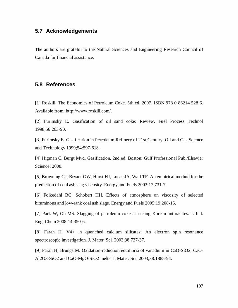
107


The authors are grateful to the Natural Sciences and Engineering Research Council of

Canada for financial assistance.

5.8 References

[1] Roskill. The Economics of Petroleum Coke. 5th ed. 2007. ISBN 978 0 86214 528 6.

Available from: http://www.roskill.com/.

[2] Furimsky E. Gasification of oil sand coke: Review. Fuel Process Technol

1998;56:263-90.

[3] Furimsky E. Gasification in Petroleum Refinery of 21st Century. Oil and Gas Science

and Technology 1999;54:597-618.

[4] Higman C, Burgt Mvd. Gasification. 2nd ed. Boston: Gulf Professional Pub./Elsevier

Science; 2008.

[5] Browning GJ, Bryant GW, Hurst HJ, Lucas JA, Wall TF. An empirical method for the

prediction of coal ash slag viscosity. Energy and Fuels 2003;17:731-7.



[7] Park W, Oh MS. Slagging of petroleum coke ash using Korean anthracites. J. Ind.

Eng. Chem 2008;14:350-6.

[8] Farah H. V4+ in quenched calcium silicates: An electron spin resonance

spectroscopic investigation. J. Mater. Sci. 2003;38:727-37.

[9] Farah H, Brungs M. Oxidation-reduction equilibria of vanadium in CaO-SiO2, CaO-

Al2O3-SiO2 and CaO-MgO-SiO2 melts. J. Mater. Sci. 2003;38:1885-94.

108

[10] Vargas S, Frandsen FJ, Dam-Johansen K. Rheological properties of high-

temperature melts of coal ashes and other silicates. Progress in Energy and Combustion

Science 2001;27:237-429.

[11] Mills KC, Chapman L, AFox AB, Sridhar S. 'Round robin' project on the estimation

of slag viscosities. Scand J Metall. 2001;30:396-403.

[12] Arvelakis S, Frandsen FJ, Folkedahl B, Hurley J. Viscosity of ashes from energy

production and municipal solid waste handling: A comparative study between two

different experimental setups. Energy and Fuels 2008;22:2948-54.



[14] Ilyushechkin AY, Hla SH, Roberts DG, Kinaev NN. The Effect of solids and phase

compositions on viscosity behaviour and Tcv of slags from Australian bituminous coals.

J. Non-Cryst. Solids 2011;357:893-902.


FactSage 2010. Available from http://www.factsage.com.

[16] French D, Hurst HJ, Marvig P. Comments on the use of molybdenum components

for slag viscosity measurements. Fuel Process Technol. 2001;72:215-25.

[17] Duchesne MA, Ilyushechkin AY, Macchi A, Anthony EJ. Optimization of Canadian

petroleum coke, coal and fluxing agent blends via slag viscosity measurements and

models. 27th Annual International Pittsburgh Coal Conference; Istanbul, Turkey, 2010.

ISBN 1-890977-27-6.

109

Chapter 6. Interactions of vanadium-rich slags with crucible materials during viscosity measurements

Accepted for publication in Journal of Materials Science (2012), DOI:

10.1007/s10853-012-6838-8

Alexander Y. Ilyushechkina, Marc A. Duchesneb, San S. Hlaa, Arturo

Macchib, Edward J. Anthonyc

aCSIRO Energy Technology, Queensland Centre for Advanced Technologies, 1

Technology Court, Pullenvale QLD 4069, Australia

bChemical and Biological Engineering Department, University of Ottawa, 161 Louis



110

6.1 Abstract

Slag chemistry is important for the assessment of flow behaviour of slags produced

during gasification of coal and coal-petroleum coke blends. Slags containing vanadium

species react readily with the crucible and spindle materials used for viscosity

measurements. Interaction of vanadium-rich slags with various materials has been

investigated in order to obtain a better understanding of the impact of containment

materials on the resulting slag chemistry and viscosity.

The bulk and phase compositions of two petroleum coke slags in Al2O3, Mo, Pt and Ni

crucibles produced under different laboratory conditions were analysed, and kinetics of

slag composition changes at 1400 °C were determined. Mechanisms of the slag

interactions with crucibles are described. They involve exchanging of crucible and slag

constituents, formation of interfaces with distinct compositions, and continuously

changing phase equilibria in the system. For slag processed in Ni and Pt crucibles,

reduction of Fe and Ni from oxide to metallic form occurs and is followed by dissolution

into the crucible materials.

Viscosity of slags with Mo, Ni and Al2O3 crucibles are determined in the temperature

range 1200-1500 °C. Resulting changes in the bulk composition of the processed slag has

an impact on the slag viscosity. At given temperatures, viscosities of the slags produced

in different crucibles are different. The impact of crucible materials and their

applicability in viscosity measurements of high-vanadium containing slags are also

discussed in order to define the optimal conditions.

Keywords: Slag, Viscosity, Petroleum coke, Gasification, Vanadium

111

6.2 Introduction

Petroleum coke (petcoke) ash can contain high concentrations of vanadium, nickel, and

iron. Vanadium oxide is a major impurity in the petcoke slags which is not found in coal

ash. Vanadium containing slags are typically produced during gasification of coal-

petroleum coke blended feed. Petcoke ash chemistry depends on the petcoke’s origin.

Vanadium concentration in petcoke ash can be as high as 75 wt.% [1]. However, total ash

content in petcoke is typically between 1-2 wt.%, while ash content in the coal is around

10 wt.%, and the total concentration of vanadium in the slags from coal-petcoke blends

depends on the feedstock blending ratio. The oxidation state of vanadium depends upon

the temperature and partial pressure of oxygen [2, 3]. Due to the low oxygen partial

pressure which may be encountered in a gasifier (O2 activity = 10-9-10-7 at temperatures

T=1300-1600 ºC [4]), a VOx phase can precipitate during gasification. Previous studies

have identified karelianite (V2O3) in slag which may increase the viscosity of a

coal/petcoke mixture [5]. Attempts to predict the effect of vanadium on viscosity have

been made using the FactSage thermodynamic package [6, 7]. However, the FactSage

databases do not consider vanadium oxide solutions which were observed in quenched

samples [7]. A recent study of phase equilibria for synthetic coal-petcoke slag mixtures in

simulated gasification conditions reported compositions of liquid and solid phases at

1500 ºC [8]. This may provide some input in the modelling of slag viscosity; however the

phase equilibria approach may not be suitable for predicting slag viscosity in vanadium-

containing slags processed in industrial conditions as it will be explained later in the

paper.

Despite the importance of real viscosity data for slags, experimentally the effect of

vanadium on the viscosity of gasification slags is rarely studied [6, 7, 9]. Major obstacles

associated with viscosity measurements of vanadium containing gasification slags are: i)

transition of oxidation states of metals in precursor materials (ashes) during slag

formation and ii) interaction of the slag with crucible materials, which may continuously

112

change phase equilibria in the system and slag bulk composition. Park and Oh [6]

obtained viscosity results for slags from a Korean anthracite blended with CaO and V2O3,

where V2O3 content in the slags did not exceed 3.4 wt.%. They highlighted the effect of

petcoke on the temperature of critical viscosity; the temperature below which viscosity

sharply increases upon further cooling. The temperature of critical viscosity was higher

in petcoke-coal ash blends compared with pure coal ashes. Viscosities of different

petcoke-coal ash blends were measured in previous studies by the current authors [7, 9].

Slag viscosity data were obtained with a high level of confidence for compositions

containing up to 5 wt.% V2O3. However, accurate viscosities of pure petcoke slags were

difficult to obtain because the compositions of these slags were significantly affected by

their interactions with crucible materials.

In the present study, interactions of vanadium-rich slags with metallic and refractory

materials are investigated. This will provide a better understanding of the impact of

metallic and refractory materials on slag chemistry. Conventional and potential crucible

materials applicable to viscosity measurements of high-vanadium containing slags

produced by gasification of petcoke and coal-petcoke blends are assessed. Results of this

work also provide some insights into the reactions and phase transformations which can

be associated to slag flow behaviour in industrial gasification conditions.

6.3 Experimental

6.3.1 Sample preparation

Two petcoke ashes and four crucible materials were used in this study. The petcoke ash

compositions and crucible materials tested are given in Table 6.1. Crucible materials

include metals: Mo (99+% purity), Ni (99%), Pt (99.99%), and high-density alumina

ceramic (99.7% ). Pelletised petcoke ashes were melted in a reducing gas atmosphere

(provided by a graphite enclosure) in flowing inert gas (nitrogen or argon). The partial

pressure of oxygen, pO2, in the system has been measured using an oxygen probe (HT

113

oxygen probe, Australian Oxytrol Systems). At temperatures between 1200-1450 °C, O2

activity values near the slag surface were detected between 2.8x10-11 – 2.9x10-9.

Table 6.1: Composition of petcoke ashes (wt.%) and crucibles used in the study

Composition P1 P2 SiO2 37.77 43.41 Al2O3 16.60 14.82 Fe2O3 7.35 9.41 TiO2 1.10 4.13 CaO 15.82 1.36 MgO 3.87 0.62 Na2O 1.67 1.13 K2O 0.96 1.75 V2O5 6.67 20.69 NiO 1.09 2.68 P2O5 <0.2 <0.2 SO3 7.11 <0.2

Crucibles P1 P2 Al2O3 + + Mo + + Ni + Pt +

Some of the slag samples were obtained prior to and after viscosity measurements

(described below). Their processing temperature profiles were similar to Profile 1

presented in Figure 6.1. Cold rod quenching experiments (Mo, Ni and Al2O3 supports) or

equilibration in envelopes (Pt support) were performed to obtain quenched slag samples

at a fixed temperature (Tq) for investigation of the kinetics of slag interaction with

support materials. Cold rod quenching involves dipping a Mo or Al2O3 rod in the molten

slag, removing it and then cooling it in water. Envelope equilibration involves heating the

slag sample in a small envelope made of the material of interest and suddenly dropping

the envelope out of the furnace into water for quenching. Temperature profiles used for

slag-crucible interaction kinetics are depicted by Profile 2 in Figure 6.1.

114

Figure 6.1: Temperature profiles used for slag preparation and processing. Profile 1 is in solid lines,

Profile 2 and quenching are in dashed lines. The shaded area corresponds to viscosity measurement.

6.3.2 Sample analysis

Slowly cooled (post-viscosity tests) and quenched slags were analysed using Scanning

Electron Microscopy (SEM) in backscattering mode. Energy Dispersive X-ray

Spectroscopy (EDS) was undertaken to identify the elemental composition of selected

regions of the slag. Electron Probe Microanalysis (EPMA) was used to identify the

composition of solid and liquid phases in the slag samples. In reducing conditions, iron

and vanadium are present in the slag as Fe2+ or Fe3+ and V2+ or V3+ respectively. EPMA

analysis provides information on the cation ratio present in the sample. However the

oxidation states of iron and vanadium in the various phases were not measured in this

study. For ease of presentation in the present study all of the iron was recalculated to the

ferric oxidation state and vanadium as V2O3.

Amounts of solids were determined using results of EPMA analysis (elements content in

the phases) of the samples and mass balances for elements, which do not participate in

slag-crucible interactions (such as Si and Ca). Bulk chemical composition of the slag and

ash were determined by Inductively Coupled Plasma - Atomic Emission Spectroscopy

(ICP-AES) or X-ray fluorescence (XRF), and confirmed by EPMA.

115

6.3.3 Viscosity measurements

Slag viscosity measurements were performed in a Carbolite 3 litre BLF1700 furnace with

a Brookfield RVDV-IIIU rheometer [7]. Petcoke ashes were placed into the crucible and

heated in a flow of argon to form liquid slag. To ensure reducing conditions, the crucible

was placed in a sacrificial graphite liner. O2 activity values are specified in section 6.3.1.

Viscosity measurements were performed using a rotating bob (made from Mo or Al2O3)

connected to the rheometer. Measurements were conducted at incremental temperature

steps (20-30 ºC) within the temperature range 1200-1500 °C. Temperature profiles where

viscosity measurements were taken are marked in Figure 1 (shaded areas). After slag pre-

melting at T1 =1225-1300 °C (sample heating rate is 5°C/min), the temperature of the

samples was increased to Tmax =1340-1500 °C. During the cooling stage (2°C/min),

samples were held at each temperature (T2) for at least 20-30 min intervals to equilibrate

temperature inside the crucible. At each temperature, the slag viscosity was measured at

least three times with various shear rates to ensure the repeatability of measurements. The

standard deviation of the measurements was below 5% of the mean value.

6.4 Results and discussion

Both petcoke slags were highly reactive with the crucibles used in this study. Interactions

of the slags with different materials were investigated in terms of the phase formations,

kinetics and mechanisms of reaction. For both petcokes, results with each crucible

material are presented below.

6.4.1 Slag processed in Al2O3

Figure 6.2 shows micrographs of the petcoke slags in an Al2O3 crucible following Profile

1 heat treatment with slow cooling. Phase compositions observed in Figure 6.2 are listed

in Table 6.2. Both samples have a clear interface phase which was identified as Al2O3

spinel. The concentration of V and Ni are higher in the interface observed for P2 than for

116

P1. This is expected since P2’s initial composition has higher concentrations of both Ni

and V. V-rich spinels are also observed with both slags, however, only Ni concentration

is higher in slag P2’s V-spinel than in slag P1’s V-spinel. Differences in the initial

petcoke ash Ca content result in differences for the other observed phases: feldspar was

formed in slag P1, while some mullite appeared in P2 slag. Molten slag has penetrated

into the Al2O3 support (up to 2 mm in depth) and formed Al2O3 spinel in the pores

between Al2O3 grains. Composition of these spinels determined by EPMA is very similar

to the composition of the interface phases ((1) and (5) in Figure 6.2) observed with each

petcoke slag. The observed microstructures in slow-cooled slags resulted from

compositional changes and reactions which occur during the whole heat treatment in

temperature Profile 1 and do not indicate at which stage of the treatment the phase

changes occurred.

Figure 6.2: Microstructures of slow cooled P1 (a) and P2 (b) slags with Al2O3 supports after

processing with Profile 1. Numbered phases are listed in Table 6.2.

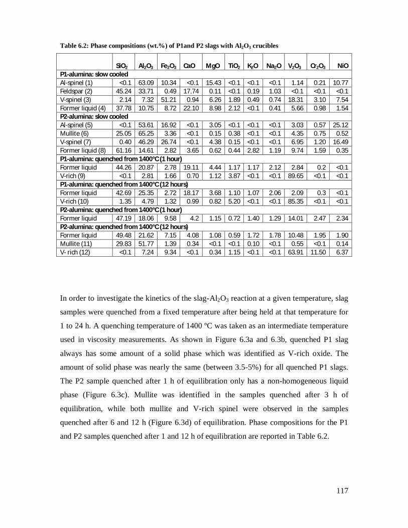
117

Table 6.2: Phase compositions (wt.%) of P1and P2 slags with Al2O3 crucibles

SiO2

Al2O3

Fe2O3

CaO

MgO

TiO2

K2O

Na2O

V2O3

Cr2O3 NiO

P1-alumina: slow cooled Al-spinel (1) <0.1 63.09 10.34 <0.1 15.43 <0.1 <0.1 <0.1 1.14 0.21 10.77 Feldspar (2) 45.24 33.71 0.49 17.74 0.11 <0.1 0.19 1.03 <0.1 <0.1 <0.1 V-spinel (3) 2.14 7.32 51.21 0.94 6.26 1.89 0.49 0.74 18.31 3.10 7.54 Former liquid (4) 37.78 10.75 8.72 22.10 8.98 2.12 <0.1 0.41 5.66 0.98 1.54 P2-alumina: slow cooled Al-spinel (5) <0.1 53.61 16.92 <0.1 3.05 <0.1 <0.1 <0.1 3.03 0.57 25.12 Mullite (6) 25.05 65.25 3.36 <0.1 0.15 0.38 <0.1 <0.1 4.35 0.75 0.52 V-spinel (7) 0.40 46.29 26.74 <0.1 4.38 0.15 <0.1 <0.1 6.95 1.20 16.49 Former liquid (8) 61.16 14.61 2.82 3.65 0.62 0.44 2.82 1.19 9.74 1.59 0.35 P1-alumina: quenched from 1400°C (1 hour) Former liquid 44.26 20.87 2.78 19.11 4.44 1.17 1.17 2.12 2.84 0.2 <0.1 V-rich (9) <0.1 2.81 1.66 0.70 1.12 3.87 <0.1 <0.1 89.65 <0.1 <0.1 P1-alumina: quenched from 1400°C (12 hours) Former liquid 42.69 25.35 2.72 18.17 3.68 1.10 1.07 2.06 2.09 0.3 <0.1 V-rich (10) 1.35 4.79 1.32 0.99 0.82 5.20 <0.1 <0.1 85.35 <0.1 <0.1 P2-alumina: quenched from 1400°C (1 hour) Former liquid 47.19 18.06 9.58 4.2 1.15 0.72 1.40 1.29 14.01 2.47 2.34 P2-alumina: quenched from 1400°C (12 hours) Former liquid 49.48 21.62 7.15 4.08 1.08 0.59 1.72 1.78 10.48 1.95 1.90 Mullite (11) 29.83 51.77 1.39 0.34 <0.1 <0.1 0.10 <0.1 0.55 <0.1 0.14 V- rich (12) <0.1 7.24 9.34 <0.1 0.34 1.15 <0.1 <0.1 63.91 11.50 6.37

In order to investigate the kinetics of the slag-Al2O3 reaction at a given temperature, slag

samples were quenched from a fixed temperature after being held at that temperature for

1 to 24 h. A quenching temperature of 1400 ºC was taken as an intermediate temperature

used in viscosity measurements. As shown in Figure 6.3a and 6.3b, quenched P1 slag

always has some amount of a solid phase which was identified as V-rich oxide. The

amount of solid phase was nearly the same (between 3.5-5%) for all quenched P1 slags.

The P2 sample quenched after 1 h of equilibration only has a non-homogeneous liquid

phase (Figure 6.3c). Mullite was identified in the samples quenched after 3 h of

equilibration, while both mullite and V-rich spinel were observed in the samples

quenched after 6 and 12 h (Figure 6.3d) of equilibration. Phase compositions for the P1

and P2 samples quenched after 1 and 12 h of equilibration are reported in Table 6.2.

118

Compositional changes in the quenched samples are mainly associated with changes in V

and Al content in the solid and liquid phases, as illustrated in Figure 6.4. Major changes

in concentrations of V and Al oxides occur in the first 3 h of equilibration. However,

continuous changes of Al2O3 and V content in the slag compositions demonstrate that

phase equilibria has not been achieved even after 12 h of equilibration. It is clear that the

Al2O3 crucible supplies extra Al in the melt while V is incorporated into the crucible.

With longer equilibration time, the slopes become flat which indicates a lower rate of V

and Al exchange between the slags and crucibles.

Figure 6.3: Microstructures of P1 and P2 slags on Al2O3 supports quenched from 1400 °C: P1 after

1h (a), P1 after 12 h (b), P2 after 1h (c), and P2 after 12h (d).

119

Figure 6.4: V2O3 and Al2O3 content in P1 (a, b) and in P2 (c, d) slags on Al2O3 supports quenched

from 1400 °C. (part 1 of 2)

120

Figure 6.4: V2O3 and Al2O3 content in P1 (a, b) and in P2 (c, d) slags on Al2O3 supports quenched

from 1400 °C. (part 2 of 2)

6.4.2 Slag processed in Mo

Micrographs of P1 and P2 slags processed in Mo crucibles with Profile 1 are shown in

Figure 6.5. The identified oxide phases are listed in Table 6.3. With P1, the corroded Mo

crucible dissolved metallic Ni from the slag and formed a layer 10-30 µm thick on the

edge of the Mo crucible (Figure 6.5a). For both P1 and P2, there is a clear interface phase

formed between the crucible (not attached to the P2 sample) and the slag, which is

identified as a Mo and V oxides solid solution, which contains small concentrations of

121

NiO, Cr2O3 and TiO2. Other solid phases observed are V-rich spinel (grey 10-50 µm

crystallites in Figure 6.5a and 6.5b) and dispersed inclusions of Mo oxide (light grey

particles in Figure 6.5a). As P2 has a higher V content (approximately three times higher)

than P1, the concentration of V at the interface is also higher (two times). More Mo was

precipitated in the V-rich oxide of sample P1, which also formed closer to the Mo-rich

interface.

Figure 6.5: Microstructures of slow cooled slags P1 (a) and P2 (b) on Mo supports after processing

with Profile 1. Numbered phases are listed in Table 6.3.

122

Table 6.3: Phase compositions (wt.%) of P1and P2 slags with Mo crucibles

SiO2

Al2O3

Fe2O3

CaO

MgO

TiO2

K2O

Na2O

V2O3

Cr2O3

NiO

MoO3

P1-Mo: slow cooled Interface (1) <0.1 <0.1 0.27 <0.1 <0.1 0.93 <0.1 <0.1 10.89 1.00 0.54 78.95 V- rich (2) <0.1 5.21 18.43 <0.1 3.78 1.46 <0.1 <0.1 49.04 3.23 2.53 20.66 Former liquid (3) 44.40 19.24 5.95 15.64 3.12 1.08 1.07 2.39 2.98 0.35 0.25 3.30 P2-Mo: slow cooled Interface (4) <0.1 <0.1 <0.1 <0.1 <0.1 0.64 <0.1 <0.1 21.73 1.94 0.21 79.59 V-rich (5) <0.1 3.25 14.20 <0.1 0.39 1.35 <0.1 <0.1 58.94 4.42 6.82 5.98 Former liquid (6) 64.38 16.31 3.74 3.45 0.87 0.25 3.04 1.43 1.36 0.23 0.42 2.72 P1-Mo: quenched from 1400°C (1 hour) V-rich (7) 0.5 3.66 2.08 0.4 0.89 3.19 <0.1 <0.1 77.91 6.23 <0.1 0.23 Former liquid 47.23 18.99 3.78 17.48 4.09 1.10 1.46 2.37 2.58 0.33 <0.1 <0.1 P1-Mo: quenched from 1400°C (12 hours) V-rich (8) <0.1 2.51 2.66 <0.1 0.84 3.78 0.03 0.00 80.45 6.05 0.10 3.05 Former liquid 44.64 18.84 5.44 18.42 4.50 1.20 1.18 2.00 2.62 0.30 <0.1 0.21 P2-Mo: quenched from 1400°C (1 hour) V-rich (9) <0.1 3.93 10.24 <0.1 0.35 0.93 <0.1 <0.1 64.90 11.72 6.64 1.11 Former liquid 45.30 16.00 7.56 4.14 1.21 0.5 1.56 1.34 13.97 2.47 2.18 3.59 P2-Mo: quenched from 1400°C (12 hours) V-rich (10) <0.1 3.63 10.77 <0.1 0.43 1.11 <0.1 <0.1 65.44 11.82 5.14 1.54 Former liquid 49.16 16.32 7.34 4.56 1.35 0.53 1.65 1.49 8.28 1.47 1.47 6.03

As was done for the Al2O3 tests, quenching experiments were conducted to investigate

the kinetics of slag-Mo crucible interaction. Samples were quenched after 15 min, 1 h, 3

h, 6 h, 12 h and 24 h of equilibration at 1400 °C. All P1 and P2 quenched slags consist of

a liquid phase and a V-rich spinel. Phase compositions of samples quenched after 1 and

12 h of equilibration are listed in Table 6.3 and shown in Figure 6.6. The quantity of

solids in the P1 slag does not change dramatically over 24 h, while gradual growth of

solids occurs with greater equilibration time for the P2 slag (Figure 6.7). The V and Mo

content in all solids, in the liquid phase, and in total for quenched P1 and P2 slags

processed in a Mo crucible are shown in Figure 6.8. In both P1 and P2 slags, the initial

concentration of V decreases rapidly in the first hour of equilibration. The V content is

partially restored after 6 and 24 h of equilibration for P1 and P2 slags, respectively. After

6 h of equilibration, the concentration of V in P1 slag continues to decrease. Over this

time, the Mo concentration in P1 slag increases from 0.4 to 3.3 wt.%. For P2 slag, the

concentration of Mo rapidly increases in the first hour of equilibration, reaches a

123

maximum of 6.3 wt.% after 6 h, and then slightly decreases in the next 18 h. The

difference in the kinetics of V depletion and Mo enrichment in P1 and P2 slags is likely

associated with the concentration of V in the initial slag. At first, the P2 slag reacts more

aggressively with the Mo support. This is seen by the rapid increase in liquid Mo content.

Past 6 h equilibration time, the Mo-V-oxide interface forms a continuous layer, as was

observed with the slowly cooled slag (Figure 6.5b). This phase still consumes Mo from

the support but resists penetration of Mo in the liquid slag. Moreover this phase may also

consume already dissolved Mo from the liquid slag (Mo decrease in bulk slag) and V

which was dissolved in the Mo support earlier. The Mo-V-oxide interface is also forming

in P1 slag but V dissolution into the crucible and Mo uptake into the slag are slower for

the first 12 h. Past 12 h, the V near the interface likely becomes depleted and Mo from

the support is no longer consumed by the interface phase growth. The discontinuous

interface phase (as observed in Figure 6.5a) allows the Mo to penetrate into the bulk slag.

124

Figure 6.6: Microstructures of P1 and P2 slags on Mo supports quenched from 1400 °C: P1 after 1h

(a), P1 after 12 h (b), P2 after 1h (c), and P2 after 12h (d).

Figure 6.7: Solid phase content in P1 and P2 slags on Mo supports quenched from 1400 °C.

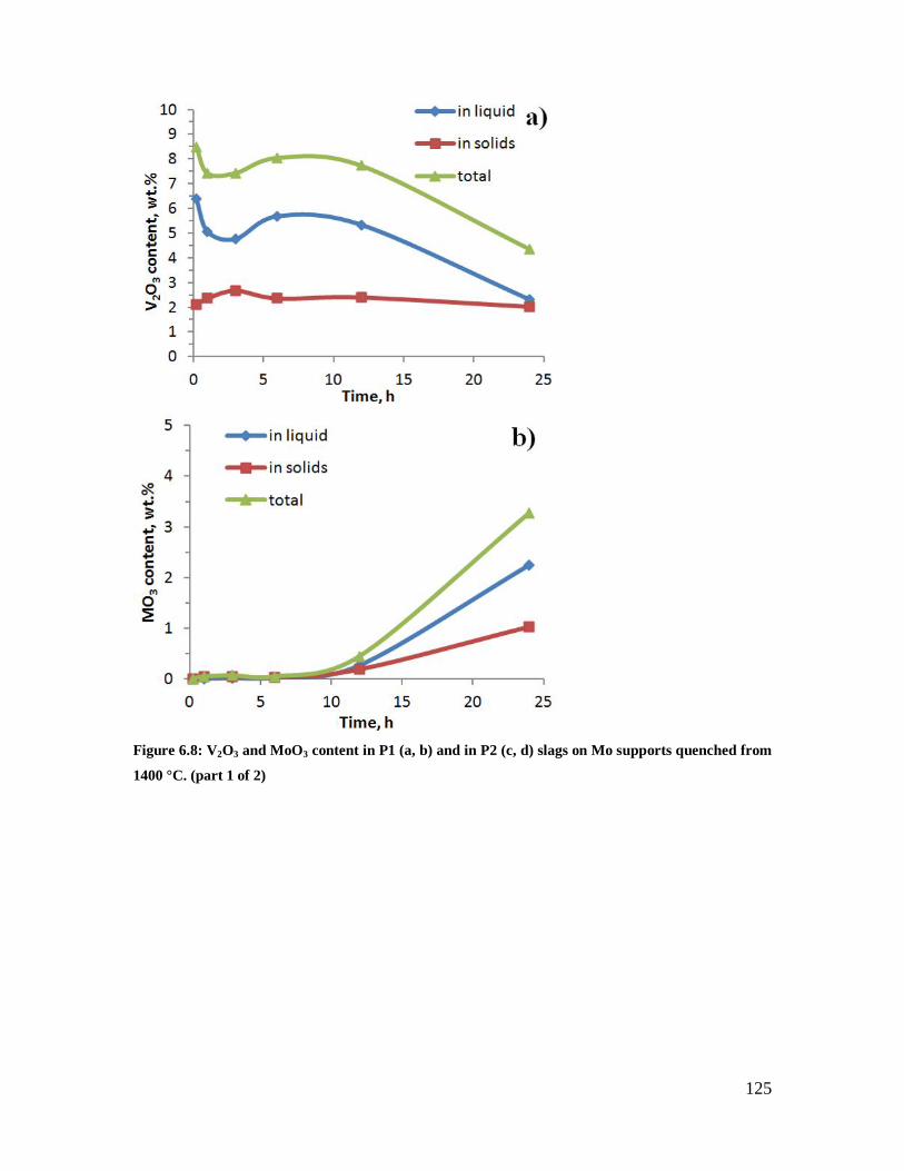
125

Figure 6.8: V2O3 and MoO3 content in P1 (a, b) and in P2 (c, d) slags on Mo supports quenched from

1400 °C. (part 1 of 2)

126

Figure 6.8: V2O3 and MoO3 content in P1 (a, b) and in P2 (c, d) slags on Mo supports quenched from

1400 °C. (part 2 of 2)

6.4.3 Slag processed in Pt or Ni

Pt and Ni were considered as alternative candidates for crucibles to be used in V-rich

slags preparation and viscosity measurements. However, both metals were found to react

with V-rich slag.

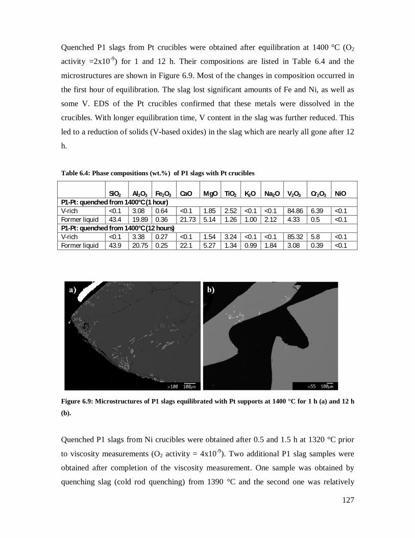
127

Quenched P1 slags from Pt crucibles were obtained after equilibration at 1400 °C (O2

activity =2x10-9) for 1 and 12 h. Their compositions are listed in Table 6.4 and the

microstructures are shown in Figure 6.9. Most of the changes in composition occurred in

the first hour of equilibration. The slag lost significant amounts of Fe and Ni, as well as

some V. EDS of the Pt crucibles confirmed that these metals were dissolved in the

crucibles. With longer equilibration time, V content in the slag was further reduced. This

led to a reduction of solids (V-based oxides) in the slag which are nearly all gone after 12

h.

Table 6.4: Phase compositions (wt.%) of P1 slags with Pt crucibles

SiO2

Al2O3

Fe2O3

CaO

MgO

TiO2

K2O

Na2O

V2O3

Cr2O3

NiO

P1-Pt: quenched from 1400°C (1 hour) V-rich <0.1 3.08 0.64 <0.1 1.85 2.52 <0.1 <0.1 84.86 6.39 <0.1 Former liquid 43.4 19.89 0.36 21.73 5.14 1.26 1.00 2.12 4.33 0.5 <0.1 P1-Pt: quenched from 1400°C (12 hours) V-rich <0.1 3.38 0.27 <0.1 1.54 3.24 <0.1 <0.1 85.32 5.8 <0.1 Former liquid 43.9 20.75 0.25 22.1 5.27 1.34 0.99 1.84 3.08 0.39 <0.1

Figure 6.9: Microstructures of P1 slags equilibrated with Pt supports at 1400 °C for 1 h (a) and 12 h

(b).

Quenched P1 slags from Ni crucibles were obtained after 0.5 and 1.5 h at 1320 °C prior

to viscosity measurements (O2 activity = 4x10-9). Two additional P1 slag samples were

obtained after completion of the viscosity measurement. One sample was obtained by

quenching slag (cold rod quenching) from 1390 °C and the second one was relatively

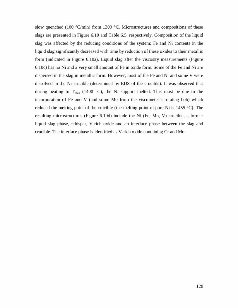
128

slow quenched (100 °C/min) from 1300 °C. Microstructures and compositions of these

slags are presented in Figure 6.10 and Table 6.5, respectively. Composition of the liquid

slag was affected by the reducing conditions of the system: Fe and Ni contents in the

liquid slag significantly decreased with time by reduction of these oxides to their metallic

form (indicated in Figure 6.10a). Liquid slag after the viscosity measurements (Figure

6.10c) has no Ni and a very small amount of Fe in oxide form. Some of the Fe and Ni are

dispersed in the slag in metallic form. However, most of the Fe and Ni and some V were

dissolved in the Ni crucible (determined by EDS of the crucible). It was observed that

during heating to Tmax (1400 °C), the Ni support melted. This must be due to the

incorporation of Fe and V (and some Mo from the viscometer’s rotating bob) which

reduced the melting point of the crucible (the melting point of pure Ni is 1455 °C). The

resulting microstructures (Figure 6.10d) include the Ni (Fe, Mo, V) crucible, a former

liquid slag phase, feldspar, V-rich oxide and an interface phase between the slag and

crucible. The interface phase is identified as V-rich oxide containing Cr and Mo.

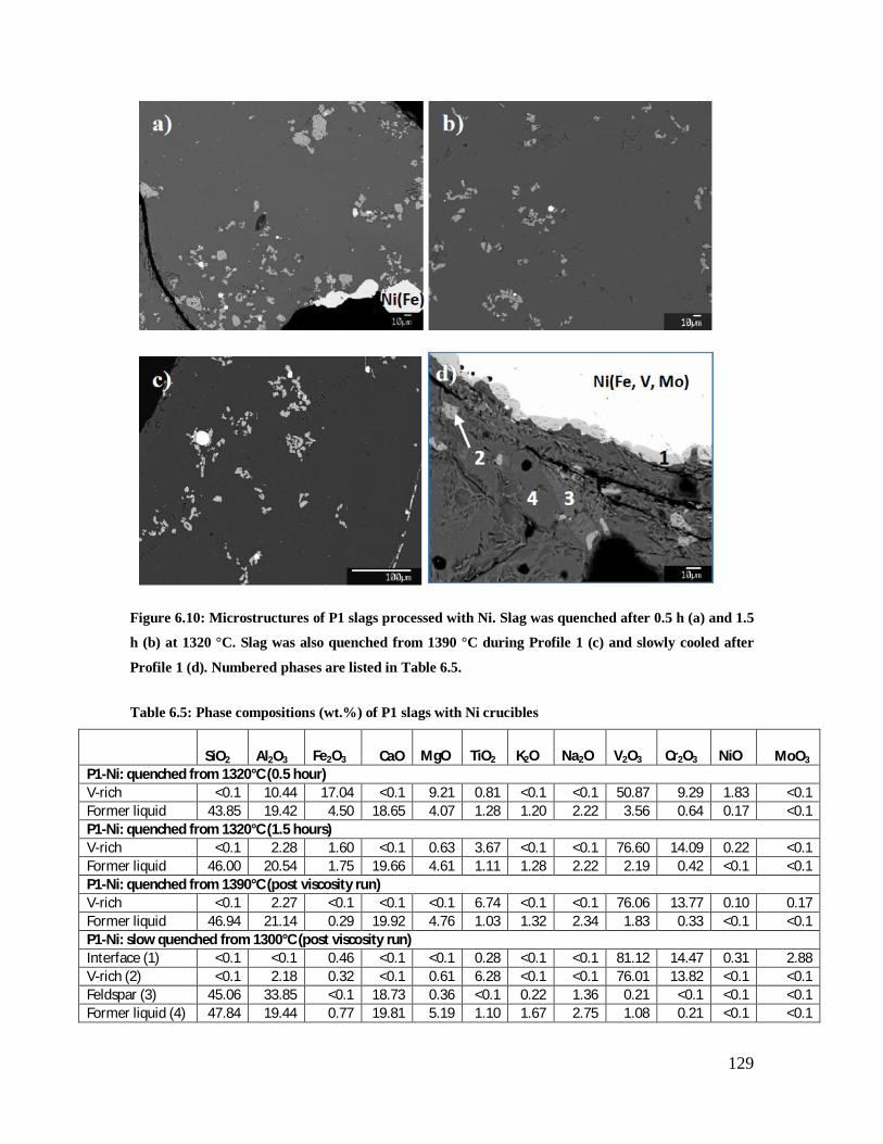
129

Figure 6.10: Microstructures of P1 slags processed with Ni. Slag was quenched after 0.5 h (a) and 1.5

h (b) at 1320 °C. Slag was also quenched from 1390 °C during Profile 1 (c) and slowly cooled after

Profile 1 (d). Numbered phases are listed in Table 6.5.

Table 6.5: Phase compositions (wt.%) of P1 slags with Ni crucibles

SiO2 Al2O3

Fe2O3 CaO

MgO

TiO2

K2O

Na2O

V2O3

Cr2O3

NiO MoO3

P1-Ni: quenched from 1320°C (0.5 hour) V-rich <0.1 10.44 17.04 <0.1 9.21 0.81 <0.1 <0.1 50.87 9.29 1.83 <0.1 Former liquid 43.85 19.42 4.50 18.65 4.07 1.28 1.20 2.22 3.56 0.64 0.17 <0.1 P1-Ni: quenched from 1320°C (1.5 hours) V-rich <0.1 2.28 1.60 <0.1 0.63 3.67 <0.1 <0.1 76.60 14.09 0.22 <0.1 Former liquid 46.00 20.54 1.75 19.66 4.61 1.11 1.28 2.22 2.19 0.42 <0.1 <0.1 P1-Ni: quenched from 1390°C (post viscosity run) V-rich <0.1 2.27 <0.1 <0.1 <0.1 6.74 <0.1 <0.1 76.06 13.77 0.10 0.17 Former liquid 46.94 21.14 0.29 19.92 4.76 1.03 1.32 2.34 1.83 0.33 <0.1 <0.1 P1-Ni: slow quenched from 1300°C (post viscosity run) Interface (1) <0.1 <0.1 0.46 <0.1 <0.1 0.28 <0.1 <0.1 81.12 14.47 0.31 2.88 V-rich (2) <0.1 2.18 0.32 <0.1 0.61 6.28 <0.1 <0.1 76.01 13.82 <0.1 <0.1 Feldspar (3) 45.06 33.85 <0.1 18.73 0.36 <0.1 0.22 1.36 0.21 <0.1 <0.1 <0.1 Former liquid (4) 47.84 19.44 0.77 19.81 5.19 1.10 1.67 2.75 1.08 0.21 <0.1 <0.1

130

Fe, Ni and V are main constituents of the V-rich phase which appeared in slags from

Al2O3 and Mo crucibles (listed in Tables 6.2 and 6.3). Extraction of Fe and Ni, and

partially of V, from the slags in Pt and Ni crucibles reduces the stability of the V-rich

phase. This leads to changes in phase equilibria in the systems and likely decreases the

liquidus temperature of the slags. However, P1 slag was less affected by these changes

when processed with a Ni crucible rather than a Pt crucible.

6.4.4 Mechanisms of slag-support interactions

Based on the observation of slag microstructures and analysis of the compositional

changes in the petcoke slags, proposed mechanisms of the slag-crucible interactions are

described.

For the slags in Al2O3 crucibles, the proposed mechanisms of interaction are illustrated in

Figure 6.11. First, V-rich melt starts to penetrate between Al2O3 grains (Figure 6.11a).

The reaction of the penetrated melt leads to dissolution of Al2O3 into the slag as well as

formation of V-spinels in the pockets (1-10 µm, as shown in Figure 6.2) between

alumina grains (Figure 6.11b). The slag still may contain some V-rich solid phases

(depending on the temperature) while a V-spinel interface is forming between the Al2O3

crucible and slag (Figure 6.11c). With longer equilibration time and/or during the slag

cooling, the spinel forms a continuous interface layer (Figure 6.11d). This interface spinel

minimises V penetration into the Al2O3 crucible. However, Al2O3 enrichment in the bulk

slag was observed over all 24 h tested. This led to changes in the amount and

composition of V-rich solids, the composition of the liquid phase and appearance/or

disappearance of other solid phases (such as mullite).

131

Figure 6.11: Mechanisms of slag interaction with Al2O3 supports. Red and yellow arrows indicate

migration of support and slag constituents respectively and the targeting areas. Different contrast of

liquid slag illustrates the compositional changes.

For slags on Mo supports, the mechanisms of slag-crucible interaction are different. With

slag melting, Ni and likely V dissolve in the Mo crucible (Figure 6.12a) and form a

metallic interface (Figure 6.12b), while Mo is oxidised and dissolves into the slag. As

melting progresses, the slag still contains some V-rich solids. Mo-V-oxide forms an

interface on the surface Mo containing residual Ni and V. (Figure 6.12c). This interface

finally forms a continuous layer, consuming Mo from the crucible and V from the

metallic slag-crucible interface and from the molten slag (Figure 6.12d). The solid phase

content in the slag (mainly V-rich oxide) depends on the initial slag bulk composition and

the temperature. Since the bulk composition continuously changes over 24 h of

equilibration, the solid phase content and solid phase composition change accordingly.

132

Figure 6.12: Mechanisms of slag interaction with Mo supports. Red and yellow arrows indicate

migration of support and slag constituents respectively and the targeting areas.

For slags with Pt and Ni supports, the mechanisms of interaction include the reduction of

Fe and Ni oxides in the slag to their metallic form. Much of the Fe and Ni, as well as

some V, was taken up by the crucibles. Most of the Fe and Ni was lost within the first 1-

1.5 h. V loss was slower. This is likely due to the fact that it is mainly present as a solid

in the conditions tested.

6.4.5 Bulk compositional changes and viscosity

As described above, the composition of the petcoke slags continuously changed during

the viscosity measurements. Table 6.6 shows the bulk slag compositions prior to and after

viscosity measurements. Compositions of slags processed in Al2O3 for viscosity tests

present a deficit of V2O3, which decrease to 3.9 wt.% in P1 slag and to 10.2 wt.% in P2

slag. Both slags accumulate Al2O3 from the crucibles. While Al2O3 content in P2 slag

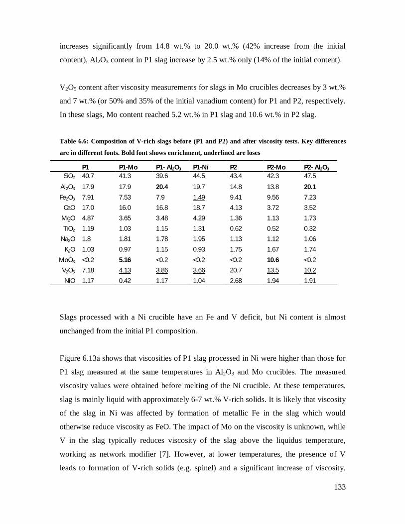
133

increases significantly from 14.8 wt.% to 20.0 wt.% (42% increase from the initial

content), Al2O3 content in P1 slag increase by 2.5 wt.% only (14% of the initial content).

V2O5 content after viscosity measurements for slags in Mo crucibles decreases by 3 wt.%

and 7 wt.% (or 50% and 35% of the initial vanadium content) for P1 and P2, respectively.

In these slags, Mo content reached 5.2 wt.% in P1 slag and 10.6 wt.% in P2 slag.

Table 6.6: Composition of V-rich slags before (P1 and P2) and after viscosity tests. Key differences

are in different fonts. Bold font shows enrichment, underlined are loses

P1 P1-Mo P1- Al2O3 P1-Ni P2 P2-Mo P2- Al2O3 SiO2 40.7 41.3 39.6 44.5 43.4 42.3 47.5

Al2O3 17.9 17.9 20.4 19.7 14.8 13.8 20.1 Fe2O3 7.91 7.53 7.9 1.49 9.41 9.56 7.23

CaO 17.0 16.0 16.8 18.7 4.13 3.72 3.52 MgO 4.87 3.65 3.48 4.29 1.36 1.13 1.73 TiO2 1.19 1.03 1.15 1.31 0.62 0.52 0.32

Na2O 1.8 1.81 1.78 1.95 1.13 1.12 1.06 K2O 1.03 0.97 1.15 0.93 1.75 1.67 1.74

MoO3 <0.2 5.16 <0.2 <0.2 <0.2 10.6 <0.2 V2O5 7.18 4.13 3.86 3.66 20.7 13.5 10.2 NiO 1.17 0.42 1.17 1.04 2.68 1.94 1.91

Slags processed with a Ni crucible have an Fe and V deficit, but Ni content is almost

unchanged from the initial P1 composition.

Figure 6.13a shows that viscosities of P1 slag processed in Ni were higher than those for

P1 slag measured at the same temperatures in Al2O3 and Mo crucibles. The measured

viscosity values were obtained before melting of the Ni crucible. At these temperatures,

slag is mainly liquid with approximately 6-7 wt.% V-rich solids. It is likely that viscosity

of the slag in Ni was affected by formation of metallic Fe in the slag which would

otherwise reduce viscosity as FeO. The impact of Mo on the viscosity is unknown, while

V in the slag typically reduces viscosity of the slag above the liquidus temperature,

working as network modifier [7]. However, at lower temperatures, the presence of V

leads to formation of V-rich solids (e.g. spinel) and a significant increase of viscosity.

134

Therefore, a decrease of V content in P1 slag likely reduces the amount of V-rich solids

formed in this system and does not lead to a sharp increase in viscosity at temperatures

below 1300 °C as is observed for P1 slag processed in Al2O3 [7]. The viscosity versus

temperature trend for this slag almost follows a simple exponential dependency on

temperature through the entire range of measurements (1200-1500 °C).

Figure 6.13: Viscosity versus temperature for P1 (a) and P2 (b) slags processed with different

support materials.

135

Of the three crucible materials tested with P1, Al2O3 provided the lowest viscosities in

the temperature range 1300-1400 °C. It is likely that at temperatures where viscosity is

mainly affected by composition of the liquid phase (above or near the liquidus

temperature), the extraction of V from the P1 slag is partially or fully compensated by

Al2O3 enrichment from interaction with the crucible. Increased Al2O3 content in the

liquid lowers the Si/Al ratio, which likely lowers the viscosity for these particular

conditions. However, at lower temperatures (<1300 °C) the excess of Al2O3 leads to

formation of spinel and a sharp increase of the viscosity.

For P2, slag viscosity measurements were conducted in Mo and Al2O3 crucibles only

(Figure 6.13b). For the slag processed in an Al2O3 crucible, viscosity values were

obtained for an extended temperature range. The measurements with a Mo crucible were

unstable since P2 slag was highly reactive with Mo and extensive reactions affected the

viscosity measurements through the entire testing procedure. The viscosity of the slag in

a Mo crucible was non-Newtonian and also significantly varied over time. For P2

processed in Al2O3, the viscosity vs. temperature trend is very similar to that of P1 slag in

Al2O3: viscosity values are low at high temperatures and follow an exponential

dependence, and then a sharp increase of viscosity is observed at temperatures below

1270 oC. Similar to P1 slag in Al2O3, this viscosity behaviour is also affected by changes

in V2O3 and Al2O3 concentrations in the slag.

It has to be noted that spindle materials (Mo and Al2O3) contacts with slag and also

contribute to slag chemistry changes. Post-viscosity measurement observations of the

spindles do not indicate significant changes in the geometry of the spindles and their

impact on viscosity value (less than 5%) does not exceed standard deviation of the

measurements.

6.4.6 Application of the results to viscosity measurements

6.4.6.1 Phase equilibrium approach Phase equilibrium considerations are used to predict flow behavior of metallurgical and

coal gasification slags [10-15]. Coal slags are often described by their four major

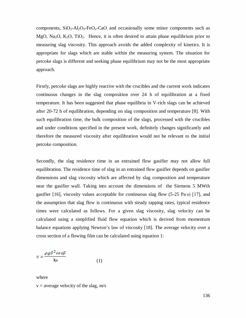
136

components, SiO2-Al2O3-FeOx-CaO, and occasionally some minor components such as

MgO, Na2O, K2O, TiO2. Hence, it is often desired to attain phase equilibrium prior to

measuring slag viscosity. This approach avoids the added complexity of kinetics. It is

appropriate for slags which are stable within the measuring system. The situation for

petcoke slags is different and seeking phase equilibrium may not be the most appropriate

approach.

Firstly, petcoke slags are highly reactive with the crucibles and the current work indicates

continuous changes in the slag composition over 24 h of equilibration at a fixed

temperature. It has been suggested that phase equilibria in V-rich slags can be achieved

after 20-72 h of equilibration, depending on slag composition and temperature [8]. With

such equilibration time, the bulk composition of the slags, processed with the crucibles

and under conditions specified in the present work, definitely changes significantly and

therefore the measured viscosity after equilibration would not be relevant to the initial

petcoke composition.

Secondly, the slag residence time in an entrained flow gasifier may not allow full

equilibration. The residence time of slag in an entrained flow gasifier depends on gasifier

dimensions and slag viscosity which are affected by slag composition and temperature

near the gasifier wall. Taking into account the dimensions of the Siemens 5 MWth

gasifier [16], viscosity values acceptable for continuous slag flow (5-25 Pa∙s) [17], and

the assumption that slag flow is continuous with steady tapping rates, typical residence

times were calculated as follows. For a given slag viscosity, slag velocity can be

calculated using a simplified fluid flow equation which is derived from momentum

balance equations applying Newton’s law of viscosity [18]. The average velocity over a

cross section of a flowing film can be calculated using equation 1:

(1)

where

v = average velocity of the slag, m/s

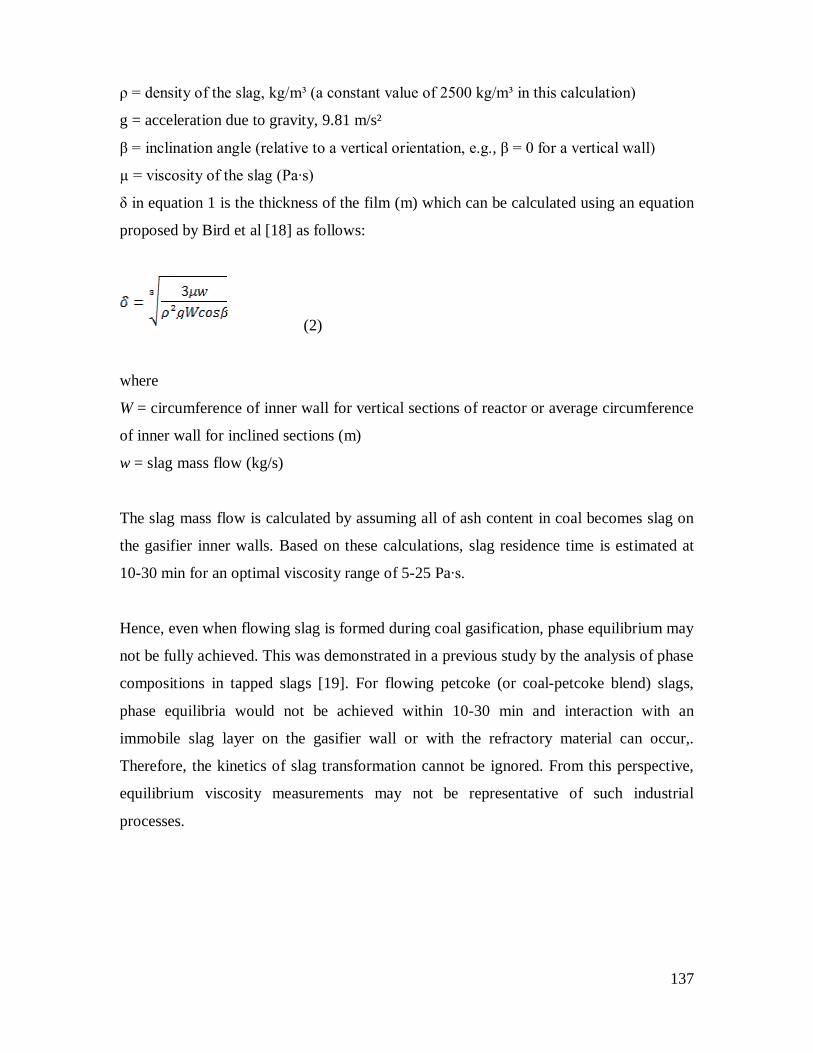
137

ρ = density of the slag, kg/m³ (a constant value of 2500 kg/m³ in this calculation)

g = acceleration due to gravity, 9.81 m/s²

β = inclination angle (relative to a vertical orientation, e.g., β = 0 for a vertical wall)

µ = viscosity of the slag (Pa∙s)

δ in equation 1 is the thickness of the film (m) which can be calculated using an equation

proposed by Bird et al [18] as follows:

(2)

where

W = circumference of inner wall for vertical sections of reactor or average circumference

of inner wall for inclined sections (m)

w = slag mass flow (kg/s)

The slag mass flow is calculated by assuming all of ash content in coal becomes slag on

the gasifier inner walls. Based on these calculations, slag residence time is estimated at

10-30 min for an optimal viscosity range of 5-25 Pa∙s.

Hence, even when flowing slag is formed during coal gasification, phase equilibrium may

not be fully achieved. This was demonstrated in a previous study by the analysis of phase

compositions in tapped slags [19]. For flowing petcoke (or coal-petcoke blend) slags,

phase equilibria would not be achieved within 10-30 min and interaction with an

immobile slag layer on the gasifier wall or with the refractory material can occur,.

Therefore, the kinetics of slag transformation cannot be ignored. From this perspective,

equilibrium viscosity measurements may not be representative of such industrial

processes.

138

6.4.6.2 Material selection Considering the four materials investigated in this work, it is evident that there is no ideal

slag crucible to be used for the viscosity measurements of petcoke slags.

Crucibles made of metals such as Pt and Ni can be used in viscosity measurements only

in less reducing conditions than relevant to the present study to avoid metallic Fe and Ni

formation. No metallic Fe precipitation and dissolution of Fe in Pt was observed when

synthetic petcoke slags were processed in Pt envelopes at 1500 °C and O2 activity =10-8

[8]. An additional limitation for Ni crucibles is temperature. Temperature has to be below

Ni’s melting point (1455 °C) or even lower if Ni dissolves some of the metals from the

slag.

Mo is a reasonable crucible material for slags containing less than 5 wt.% V2O3. It was

demonstrated that for these slags, the contamination of Mo and loss of V do not

significantly affect viscosity. For slag containing 5-10 wt.% V2O3, the measurements are

possible but the results have to be considered in context of the compositional changes.

With higher V concentrations, Mo should not be used for viscosity measurements.

However, in practice most petcokes are blended with coal in gasification. Since the ash

content of petcoke is significantly lower than the ash content of coal, it is likely that the

V2O3 of most coal-petcoke blend ashes will be below 10 wt.%.

Al2O3 has an advantage over other materials since it is usually a major component of

petcoke ashes. Therefore, the contamination from the crucible only changes a balance of

base elements in the petcoke system. V losses to the crucible are significant but about

half of the initial concentration has been conserved during viscosity tests conducted in

this study. One option to perform viscosity measurements with high V content melts is to

design artificial petcoke ashes with excess V and a deficit in Al. The excess V and Al

deficit would compensate the changes in Al and V concentrations during slag viscosity

measurements. This approach can be taken for research requiring phase equilibria. The

current study indicates that Al-V spinel forms an interface between the slag and Al2O3

crucible. This interface decreases migration of the slag to the crucible, and Al2O3 to the

slag liquid phase. Therefore, the slags with excess V will eventually be equilibrated with

139

a spinel primary phase field, while the rest of the slag may contain the liquid phase in

equilibria with other solid phases (eg. other V-rich phases and/or mullite). For this

equilibrated system the viscosity can be measured at a specified temperature for only one

specified bulk slag composition which consists of the liquid slag and solids in the liquid

slag (i.e. not including the spinel interface). With temperature changes, the equilibrium

between the interface and the rest of the slag will change. As a result, the composition of

the liquid and solids within the slag, and therefore the bulk slag composition (excluding

the interface) will change accordingly.

In entrained flow gasification, the reaction of V-containing slags with immobile slag on

the gasifier wall (for water-cooled walls) or with gasifier refractory [20] has to be

considered. To assess petcoke slag flow in industrial processes, a crucible material which

reproduces the contacting material in the process may be most suitable. This is a potential

experimental avenue to be explored.

6.5 Conclusion

Petcoke slags containing 6-21 wt.% V2O5 were found to be highly reactive with the

crucible materials used in this study. The interaction of slag with the crucibles always

involves the transfer of slag constituents to the crucible. For Mo and Al2O3 crucibles, the

interactions also include dissolution of the crucible material into the slag.

Slag equilibration at temperatures just below the liquidus temperature of slags indicates

that the investigated compositions are located in a V-rich oxide primary phase field.

Interactions of slag and crucible materials lead to changes in bulk slag composition and

appearance of new solid phases. An interface layer between the slag and crucible was

formed and identified as V-rich oxide, Mo-V-oxide and spinel for slags processed with

Ni, Mo and Al2O3 respectively. The interface layer can act as a barrier for migration of

the slag components to the crucibles and elements of the crucibles to the slags.

140

Compositional changes in the slags have an impact on viscosity and lead to differences in

viscosities of slags produced with different crucibles.

The results of this study indicate that for slags generated during petcoke gasification,

kinetics of the slag formation and slag interactions with immobile slag or refractory have

to be considered.

Conditions for use of a particular crucible material for slag viscosity measurements are

specified as:

- Ni and Pt crucibles can be used for viscosity tests at low reducing conditions

where formation of metallic Fe and Ni can be minimised or avoided;

- Mo supports can be used for viscosity measurements where the total

concentration of V2O3 in the petcoke (or coal-petcoke blend) ash is less than 5

wt.%;

- Al2O3 crucibles can be used for slags with higher than 5 wt.% V2O3.

However, the starting mixture has to be modified in order to compensate for

changes in Al and V concentrations in the slag during viscosity tests.

6.6 References

[1] Bryers RW. Utilization of petroleum coke and petroleum coke/coal blends as a means

of steam raising. Fuel Process Technol 1995;44:121–41.

[2] Farah HJ, Brungs M. V4+ in quenched calcium silicates: An electron spin resonance

spectroscopic investigation. J Mater Sci 2003;38:727-37.

[3] Farah HJ, Brungs M. Oxidation-reduction equilibria of vanadium in CaO-SiO2, CaO-

Al2O3-SiO2 and CaO-MgO-SiO2. J Mater Sci 2003;38:1885–94.

[4] Kwong K, Petty A, Bennett J, Krabbe R, Thomas H. Wear mechanisms of chromia

refractories in slagging gasifiers. Int J Appl Ceram Technol 2007;4:503–13.

141

[5] Nakano J, Sridhar S, Moss T, Bennett J, Kwong K-S. Crystallization of synthetic

coal-petcoke slag mixtures simulating those encountered in entrained bed slagging

gasifiers. Energy & Fuels 2009;23:4723–33.

[6] Park W, Oh MS. Slagging of petroleum coke ash using Korean anthracites. J Ind Eng

Chem 2008;14:350-6.

[7] Duchesne MA, Ilyushechkin AY, Hughes RW, Lu DY, McCalden DJ, Macchi A,

Anthony EJ. Flow behaviour of slags from coal and petroleum coke blends. Fuel

2012;97:321-8.

[8] Nakano J, Kwong K-S, Bennett J, Lam T, Fernandez L, Komolwit P, Sridhar S. Phase

equilibria of synthetic coal-petcoke slags (Al2O3 – CaO – FeO - V2O3) under simulated

gasification conditions. Energy & Fuels 2011;25:3298-306.

[9] Duchesne MA, Ilyushechkin AY, Macchi A, Anthony EJ. Optimization of Canadian

petroleum coke, coal and fluxing agent blends via slag viscosity measurements and

models Proceedings – 27th Annual International Pittsburgh Coal Conference, Pittsburgh,

United States, 2010;38-2.

[10] Kondratiev A, Jak E, Hayes PC. Prediction of slag viscosities in metallurgical

systems. JOM 2002;54:41-5.

[11] Kondratiev A, Jak E. Predicting coal ash slag flow characteristics (viscosity model

in the Al2O3-CaO-"FeO"-SiO2 system). Fuel 2001;80:1989-2000.

[12] Iida T. A model for accurate viscosity predictions of various types of molten slags

and glasses, in Aune RE and Sridhar S (Eds.) Proceedings of the Mills Symposium.

London, National Physical Laboratory, Teddington, UK, 2002.

[13] Zhang L, Jahanshahi S. Review and Modeling of Viscosity of Silicate Melts: Part I.

Viscosity of Binary and Ternary Silicates Containing CaO, MgO and MnO. Met Trans B

1998;29B:177–86.

[14] Hu H, Reddy RG. Modeling of Viscosities of Binary Alkaline-Earth Metal Oxide

and Silica Melts. High Temp Sci 1990;28:195–202.

[15] Muller J, Erwee M. Blast furnace control using slag viscosities and liquidus

temperatures with phase equilibria calculations, in Jones RT and den Hoed P (Eds.)

142

Southern African Pyrometallurgy 2011, Southern African Institute of Mining and

Metallurgy, Johannesburg, 2011.

[16] Hla SS, Roberts DG, Harris DJ. Integrating coal gasification performance data into

gasifiers models for IGCC-CCS systems. Final report for ACARP project CCSDRes001,

2011.

[17] Patterson JH, Hurst HJ. Ash and slag qualities of Australian bituminous coals for use

in slagging gasifiers. Fuel 2000;79:1671-8.

[18] Bird RB, Stewart WE, Lightfoot EN, Transport Phenomena, 2nd edition. John Wiley

& Sons, Inc., 2002.

[19] Roberts D, Ilyushechkin A, Tremel A, Beavis P, Kochanek M, Harris D.

Gasification of Australian Coals. Final report for ACARP Project C17060B, 2010.

[20] Rawers J, Iverson L, Collins K. Initial stages of coal slag interaction with high

chromia sesquioxide refractories. J Mater Sci 2002;37:531-8.

143

Chapter 7. Fate of inorganic matter in entrained-flow slagging gasifiers: Fuel characterization

Submitted for publication in Fuel Processing Technology (2012)

Marc A. Duchesnea, Ajae D. Hallb, Robin W. Hughesb, David J. McCaldenb,

Edward J. Anthonyb, Arturo Macchia



bCanmetENERGY, 1 Haanel Drive, Ottawa, Ontario, Canada, K1A 1M1

144

7.1 Abstract

This study is the first of a three-part research program which involves fuel

characterization, testing in a 1 MWth gasifier, and computational fluid dynamics (CFD)

modeling for entrained-flow slagging gasification. Focus is on the behaviour of inorganic

fuel components since the end goal is to develop a CFD model which includes inorganic

matter transformations. Initially, four coals were selected for this program and one

limestone was also chosen to act as a fluxing agent. Fuel properties related to ash particle

formation, gas-particle transport, particle sticking, slag flow and slag-refractory

interaction are provided with prioritization based on their potential application for

screening of potential fuels, ensuring proper gasifier operation, gasifier design and/or

CFD modeling. The selection of one or multiple experimental and/or modeling

techniques is justified and applied to determine each relevant property. Of the four coals

tested, one was deemed unsuitable based on initial screening tests. Two of the three

remaining coals require fluxing for proper gasifier operation. Design tests showed that

alumina is preferred over silicon carbide and alumina-chromia (with 30 wt.% chromia)

for use as refractory material with the selected fuels. Characterization for CFD modeling

is also discussed with results provided as supplementary data.

Keywords: Gasification, Inorganic, Mineral, Ash, Slag, CFD model

145

7.2 Introduction

Fuel and product flexibility have always been some of gasification’s selling points. More

recently, concerns over reducing emissions in industry and the power sector have

renewed interest in this technology. In comparison with coal combustion systems, the

advantages of coal gasification include high efficiency, suitability for carbon capture,

relatively easy removal of sulphur oxides, nitrogen oxides and trace contaminants, and

low water consumption [1]. Most of the successful high throughput coal gasifiers

developed in the past 60 years are of the entrained-flow slagging type [2]. This study is

the first part of a three-part research program which involves fuel characterization, testing

in a 1 MWth gasifier, and computational fluid dynamics (CFD) modeling for entrained-

flow slagging gasification. Here, the focus is on the behaviour of inorganic fuel

components as this is still ill-understood even though it can be the determining factor in

designing and operating entrained-flow gasifiers [3]. For instance, fouling or plugging of

the gasifier by inorganic matter is a major concern. Refractory wear, which is largely

dictated by interaction with inorganic matter, leads to poor plant availability. Also, the

distribution of potentially toxic inorganic matter in fly ash and slag is an environmental

concern. Four coals were selected for this program. One limestone was also selected to

act as a fluxing agent to reduce slag viscosity if required for operation with any of the

coals. F1 fuel is a lignite coal from Saskatchewan, Canada. F2 fuel is a sub-bituminous

coal from Alberta, Canada. F3 fuel is a beneficiated version of F2 with reduced ash

content. F4 fuel is another sub-bituminous coal from Alberta, Canada. L1 is a limestone

from a Canadian power company. The characterization of the fuels is described in this

study. Some bench-scale tests and models which do not relate to inorganic matter

transformations are not included. For example, thermogravimetric analysis of the fuels

can be used to optimize gasifier performance based on fuel reactivity, but is not directly

related to inorganic matter transformations and is therefore not included.

146

Selection of fuel analyses depends on the intended application of the results: (i) screening

of potential fuels; (ii) proper gasifier operation; (iii) gasifier design; and/or (iv) CFD

modeling. Unless an accurate CFD model is readily available, fuel screening, gasifier

operation and gasifier design will only make use of a subset of the tests required for CFD

modeling. A comprehensive CFD model must consider all relevant inorganic matter

phenomena, including ash particle formation, gas-particle transport, particle sticking, slag

flow and slag-refractory interaction. The properties involved are listed in Table 7.1 along

with their associated phenomena and experimental tests and models used to determine

them. The likely applications of each property are given in the last column of Table 7.1.

Since the end goal of this research program is to develop a CFD model which includes

inorganic matter transformations, a test or model for each property must be used. In Table

7.1, experimental and modeling techniques underlined and in red font were applied in this

study. Although modeling techniques generally require less time and resources,

experimental techniques are preferred where model accuracies are poor and/or the

property is very important for gasifier design and/or operation (e.g., slag viscosity). The

reasoning for the selection of each technique or model used is included in the discussion.

Properties related to screening were determined first, followed by the properties related to

operation, design, and finally CFD modeling. Results pertaining to screening, operation

and design are supplied directly in the paper. For brevity's sake, results which only

pertain to CFD modeling are provided as supplementary information. However, the

methods and importance of all results are discussed with references which demonstrate

the use of each property in CFD modeling.

147

Table 7.1: Fuel properties involved in inorganic matter phenomena

Property Phenomenaa Experimental Model Applicationsb

fuel composition 1 ultimate analysis, proximate analysis, calorimetry N/A S. O, D, M

fuel form 1 coal petrography, CCSEM ultimate/proximate models M

fuel particle size 1, 2, 3 sieving, laser diffraction, CCSEM N/A M

inorganic composition 1, 2, 3, 4, 5 XRF, XRD, CCSEM N/A S. O, D, M

inorganic form 1 XRD, HT-XRD FactSage M

inorganic particle size 1, 2, 3 CCSEM N/A M

fuel-inorganic associations 1 CCSEM, chemical fractionation N/A M

ash melting temperatures 3, 4 AFT composition models, FactSage S. O, D, M

slag viscosity 3, 4, 5 rheology composition models O, D, M

slag-refractory reactivity 4, 5 cup tests, sessile drop FactSage, numerical diffusion models D, M

slag interfacial tension 3, 5 sessile drop composition models M

inorganic density 1, 2, 3, 4, 5 pycnometry, buoyancy, dilatometer, sessile drop composition models M

inorganic heat capacity 1, 4, 5 calorimetry composition models, FactSage M

inorganic heat conductivity 1, 4, 5 various techniques with heating and temperature measurements

temperature models, thermal diffusivity models M

inorganic emissivity 1, 4 FTIR constant value from literature M a) Phenomena are coded as (1) ash particle formation, (2) gas-particle transport, (3) particle sticking, (4) slag flow and (5) slag-refractory interaction.

b) Applications are coded as (S) screening, (O) operation, (D) design and (M) CFD modeling. 147

148

7.3 Experimental

7.3.1 FactSage modeling

FactSage software predicts equilibrium solid-liquid-gas phases and compositions based

on Gibbs free energy minimization [4]. Gibbs free energy is calculated from optimized

models with parameters based on empirical data with various compositions, temperatures

and pressures. This information is contained within compound and solution databases

which must be carefully selected prior to equilibrium calculations. The FactSage 6.2

Equilib module was utilized with the FACT53 and FToxid databases. Oxide components

representing less than 1 wt.% for all samples were excluded. Sulphur is not included in

the analyses as it is expected to completely devolatilize at the temperatures of interest.

All gas and solid compounds were considered. For compounds found in both the

FACT53 and FToxid databases, preference was given to the FToxid database to have

better thermodynamic consistency with the solution phases data. Pure liquid Fe was also

considered. All solution phases were considered. However, only the SLAGA solution

was allowed to form multiple immiscible phases. Total pressure was specified at 1 atm

and, unless otherwise noted, the activity of O2 in the gas phase was set to 10-9 which is

similar to what is typically encountered near the walls in a gasifier [5].

7.3.2 Slag viscosity measurements

Artificial ashes were prepared by mixing laboratory or analytical grade Al2O3, CaCO3,

Fe2O3, K2CO3, MgCO3, Na2CO3, SiO2 and TiO2 powders. Slag viscosity measurements

were performed in a Carbolite 3 litre BLF1700 furnace with a Brookfield RVDV-IIIU

rheometer. Both the furnace and the rheometer were connected to a personal computer for

external control and data collection. Samples were placed in a molybdenum crucible. The

crucible was placed in a custom-built alumina chamber within the furnace for gas

atmosphere control and spill protection. A type B thermocouple was inserted into the

149

chamber to monitor the sample temperature. Argon flowed at 0.4 dm3/min (STP) into the

alumina chamber and a graphite sleeve was placed around the molybdenum crucible to

consume trace oxygen. Mössbauer spectroscopy of a slag sample after viscosity

measurements indicated that the iron components were in the ferrous state, confirming

the reducing nature of the experimental conditions. A molybdenum spindle was attached

to the rheometer and lowered until it sufficiently penetrated into the slag sample for the

purpose of accurate viscosity measurement. It was rotated while measuring the torque

required for spindle rotation at a given angular velocity. The operation of the rheometer

was validated with the National Institute of Standards and Technology's (NIST, United

States) standard reference material 717a. Artificial ash samples were first heated to 1225

°C and left overnight for equilibration. They were then heated to 1525-1600 °C.

Measurements were conducted at incremental temperature reduction steps. The cooling

step for each set of measurements included a reduction in temperature of 25 ºC with a

minimum of 25 minute intervals to allow the temperatures and compositions to

equilibrate inside the crucible. At each temperature, viscosity was measured multiple

times at various rotational speeds to detect non-Newtonian behaviour [6]. The final

measured value was taken at approximately 80-90% of the rheometer’s maximum torque.

7.3.3 Cup tests for slag-refractory reactivity

Approximately 0.5 g of ash was placed on 1200 mm2 pieces of refractory. The crucible

was placed in a custom-built alumina chamber within a Carbolite 3 litre BLF1700

furnace for gas atmosphere control and spill protection. A type B thermocouple was

inserted into the chamber to monitor the sample temperature. Argon was fed at 0.4

dm3/min and small pieces of graphite were placed near the samples to consume any trace

oxygen. Mössbauer spectroscopy of a slag sample after testing indicated that all the iron

atoms are in the ferrous state, confirming the reducing nature of the experimental

conditions. Samples were either heated to 1250 or 1500 °C at approximately 3 °C/min.

They were then held at the temperature of interest for 4 h and afterwards, the samples

were cooled at approximately 5 °C/min to 1100 °C and then slowly cooled to room

temperature. The slag-covered refractory was cross-sectioned using a Buhler ISOMET

150

low speed saw with a 0.4 mm 15LC wafering blade. The samples were mounted with

carbon tape on an aluminum holder. Scanning electron microscopy with energy-

dispersive X-ray spectroscopy (SEM-EDX) analysis was done using a Hitachi 3400N

VP-SEM with Oxford Instruments Si(Li) Pentafet Plus 10 mm2 detector. The system was

operated at a reduced vacuum of 30 Pa to reduce charging from the uncoated samples.

Imaging and analyses were done at 20 kV and approximately 60 µA emission current. X-

ray acquisition was done with Oxford INCA Point and ID and Mapping modules.

7.3.4 Coal petrography to determine fuel form

Coal samples (< 0.85 mm) were made into polished 25.4 mm diameter coal pellets for

microscopical analysis by reflected light as per ASTM D 2797-11a. Petrographic analysis

included (i) determination of v-type groups, percent reflectance of vitrinite and Romax as

per ASTM D 2798-11a and (ii) determination of the volume percent of macerals or

coalified organic remains as per ASTM D 2799-05a. Vitrinite reflectance was performed

with a Zeiss microscope photometer equipped with a polarizer using a 40x oil immersion

objective, 12.5x oculars, a tube factor of 1.6 and total magnification of 800x. In this

work 100 readings on vitrinite macerals covering the entire pellet surface were recorded.

Identification and point counting of coal macerals was done using a Leitz S 544-21

microscope; 50x oil immersion objective, 10x oculars, tube factor of 1.6, total

magnification of 800x. 1000 maceral counts were made on the entire polished pellet

surface.

7.3.5 CCSEM

Computer-controlled scanning electron microscopy (CCSEM) samples were mounted in

carnauba wax and carbon coated. The wax mount was glued to an epoxy blank for

structural strength. Analysis was done using a Hitachi 3400N VP-SEM with Oxford

Instruments Si(Li) Pentafet Plus 10 mm2 detector. The system was operated at full

vacuum. Imaging and analyses were done at 20 kV and approximately 60 µA emission

current. X-ray acquisition was done with Oxford INCA Feature software. Three analyses

151

were conducted per sample, all using the backscatter detector to provide elemental

contrast in the image. The first was 10,000 particles acquired at 500x magnification. This

collected particles over 10 pixels in size (0.89 µm equivalent circle diameter) and under 5

µm in breadth. A 200x magnification analysis was done over the same area as the 500x

run to collect particles over 5 µm but under 30 µm breadth. Particles over 30 µm breadth

were collected over the same area at 75x magnification. Energy-dispersive X-ray

spectroscopy (EDX) data was collected for 5 seconds per particle, at the center of the

longest chord. Each hour the quantification optimization was performed with cobalt. Two

particle detection grey level ranges were used and set manually before each analysis. For

the limestone sample, only 1 grey level range was used. Coal particles were kept separate

from mineral particles during the automated detection. Remove edge touching, two erode,

one dilate and hole fill filter options were used in the image processing to help separate

particles that were close to each other. All three magnifications were combined and the

data was sorted. Coal particles were identified by grey-level analysis; all particles below

a grey level determined at the start of the analysis were classed as coal. The remaining

particles were classified by their elemental composition. C was excluded due to the high

background, and O was calculated using the O by stoichiometry option. Quantification

was done with the base Oxford factors, no additional standards were used.

7.3.6 Other methods

ASTM D7582 was applied for determination of moisture, secondary moisture, ash and

fixed carbon in the proximate analyses. ISO 562 was applied for determination of volatile

matter in the proximate analyses. ASTM D5373 was applied for determination of carbon,

hydrogen and nitrogen in the ultimate analyses. ASTM D4239 was applied for

determination of sulphur in the ultimate analyses, while oxygen was calculated by

difference. ISO 1928 was applied to determine the gross calorific value of samples.

ASTM D1857 was applied for determination of ash fusion temperatures. ASTM D4326

was applied to determine major and minor oxides content via X-ray fluorescence (XRF).

Particle size analysis was conducted using a combination of sieving (grains > 2 mm),

152

Camsizer (grains 0.063-2 mm) and a Lecotrac LT100 Particle Size Analyzer (grains <

0.063 mm).

Quantitative X-ray diffraction (XRD) analysis of the samples was performed over the

angular range of 7 to 80° (2θ). Each sample was mixed with an internal standard. The

resulting mixture was thoroughly ground using a mortar and pestle to ensure sample

homogeneity. Integrated intensities for strong diffracting peaks of each phase were

obtained using JADE version 7.0 XRD processing software. Concentrations of the

chemicals identified in each sample were calculated using the reference intensity ratio

(RIR) method.


7.4.1 Screening

When multiple fuels are available and the gasification system in question need not rely on

all of them, routine standardized tests and simple models can be applied to the fuels for

screening. This step can reduce the number of fuels to be examined in the often more

difficult and expensive tests and models for gasifier operation, design and CFD modeling.

In this study, fuel composition, inorganic composition and ash melting temperatures have

been selected for fuel screening.

Fuel composition is directly involved in only one inorganic matter phenomenon, ash

particle formation. However, it is an indicator of two important fuel selection criteria,

energy content and reactivity. In terms of gasifier operation, the fuel composition is

required to determine fuel and fluxant mixing ratios. In terms of gasifier design,

emissions can be estimated from the fuel composition and this will impact downstream

processing. Also, CFD models rely on fuel composition for mass and energy balances.

The proximate analysis, ultimate analysis and gross calorific value for the fuels in this

153

study are given in Table 7.2. The volatiles content from the proximate analysis can be

correlated to reactivity [7]. The gross calorific value provides the energy content.

Inorganic matter composition is directly involved in all the inorganic matter phenomena.

This property is an input to models for all properties which can be determined by

FactSage or composition models (see Table 7.1) including the ash melting temperatures

which are used for fuel screening. There are different options to experimentally

determine inorganic matter composition. Quantitative XRD can be used for crystalline

materials, but it fails to determine the composition of amorphous components. CCSEM is

an option, but it is not a standardized technique. Hence, XRF was selected in this study

and the results are presented in Table 7.3. It should be noted that the bulk inorganic

matter composition is sufficient for screening, design and operation, but the composition

of specific particles may be preferred for CFD modeling.

Table 7.2: Proximate analysis, ultimate analysis and gross calorific value

F1 F2 F3 F4

Proximate Analysis Moisture (wt.%) 6.43 2.86 3.32 6.08 Ash (wt.%) 13.87 32.84 10.52 24.72 Volatile (wt.%) 36.27 27.30 34.76 26.87 Fixed Carbon (wt.%) 43.43 37.00 51.40 42.33

Ultimate Analysis Carbon (wt.%) 57.7 48.8 67.8 52.2 Hydrogen (wt.%) 3.64 3.00 4.22 3.05 Nitrogen (wt.%) 1.02 0.64 0.86 0.79 Sulphur (wt.%) 0.93 0.18 0.27 0.30 Oxygen (wt.%) 16.41 11.67 13.01 12.85

Gross Calorific Value (MJ/kg) 22.15 18.83 26.67 19.98

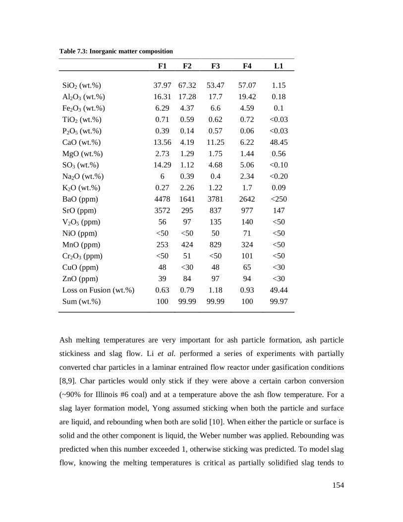
154

Table 7.3: Inorganic matter composition

F1 F2 F3 F4 L1

SiO2 (wt.%) 37.97 67.32 53.47 57.07 1.15 Al2O3 (wt.%) 16.31 17.28 17.7 19.42 0.18 Fe2O3 (wt.%) 6.29 4.37 6.6 4.59 0.1 TiO2 (wt.%) 0.71 0.59 0.62 0.72 <0.03 P2O5 (wt.%) 0.39 0.14 0.57 0.06 <0.03 CaO (wt.%) 13.56 4.19 11.25 6.22 48.45 MgO (wt.%) 2.73 1.29 1.75 1.44 0.56 SO3 (wt.%) 14.29 1.12 4.68 5.06 <0.10 Na2O (wt.%) 6 0.39 0.4 2.34 <0.20 K2O (wt.%) 0.27 2.26 1.22 1.7 0.09 BaO (ppm) 4478 1641 3781 2642 <250 SrO (ppm) 3572 295 837 977 147 V2O5 (ppm) 56 97 135 140 <50 NiO (ppm) <50 <50 50 71 <50 MnO (ppm) 253 424 829 324 <50 Cr2O3 (ppm) <50 51 <50 101 <50 CuO (ppm) 48 <30 48 65 <30 ZnO (ppm) 39 84 97 94 <30 Loss on Fusion (wt.%) 0.63 0.79 1.18 0.93 49.44 Sum (wt.%) 100 99.99 99.99 100 99.97

Ash melting temperatures are very important for ash particle formation, ash particle

stickiness and slag flow. Li et al. performed a series of experiments with partially

converted char particles in a laminar entrained flow reactor under gasification conditions

[8,9]. Char particles would only stick if they were above a certain carbon conversion

(~90% for Illinois #6 coal) and at a temperature above the ash flow temperature. For a

slag layer formation model, Yong assumed sticking when both the particle and surface

are liquid, and rebounding when both are solid [10]. When either the particle or surface is

solid and the other component is liquid, the Weber number was applied. Rebounding was

predicted when this number exceeded 1, otherwise sticking was predicted. To model slag

flow, knowing the melting temperatures is critical as partially solidified slag tends to

155

have a much higher viscosity than fully molten slag and may display non-Newtonian

behaviour [6], while fully solidified slag will not flow at all. In terms of fuel screening, a

high melting temperature indicates a poor candidate for gasification. However, low

melting temperatures do not guarantee the fuel’s slag will flow well, since the viscosity

may still be high. Slag viscosity tests may be used for screening, but slag viscosity

measurements are difficult and existing models are often unreliable [11]. The melting

temperatures can impact operation as temperature in the gasifier may be controlled to

specifically avoid solidification. They may also affect design of the gasifier as it may

impact reactivity with the refractory material. Ash fusion temperatures (AFTs) are

determined by ashing a fuel via a standard procedure, forming a cone, pyramid or cube

with the ash, and observing the deformation of the molded ash as it is heated up. The

procedure is widely employed, standardized and inexpensive. AFTs are used as indicators

of degrees of melting for the ash at different temperatures, and it is often assumed that the

ash is fully molten at the highest AFT (the flow temperature). However, solids may be

present at all fusion temperatures provided by the standard methods. Also, some ash

minerals may melt at a given temperature, then react with other molten minerals at a

higher temperature and form solids [12]. Factors other than liquid fraction, such as

surface tension, will affect the shape of the mold. Since AFTs are determined upon

heating of the ash, they are most applicable to ash particle formation and stickiness. AFTs

for this study’s fuels are given in Table 7.4. Reactor plugging usually happens with

cooling of slag as it contacts the refractory and flows down towards the cooler slag tap.

Solidification behaviour can be very different from melting [7]. If equilibrium can be

assumed during cooling, FactSage predictions are appropriate. However, these are subject

to modeling error. The mass fraction of solids in the slags of each fuel, as predicted using

FactSage, are plotted in Figure 7.1.

156

Table 7.4: Ash fusion temperatures in °C

F1 F2 F3 F4

Oxidizing Initial 1191 1254 1238 1196 Spherical 1268 1332 1274 1279 Hemispherical 1299 1385 1313 1327 Fluid 1332 >1510 1416 1457

Reducing Initial 1096 1213 1177 1191 Spherical 1107 1293 1263 1246 Hemispherical 1118 1393 1324 1310 Fluid 1177 >1510 1374 1446

0

0.1

0.2

0.3

0.4

0.5

0.6

0.7

0.8

0.9

1

1100 1150 1200 1250 1300 1350 1400 1450 1500 1550 1600

Temperature (°C)

Solid

s mas

s fra

ctio

n

F1F2F3F4F3L1F4L1

Figure 7.1: Solids mass fractions predicted using FactSage.

F1 and F3 have higher volatile content which may result in better reactivity, higher gross

calorific values which would provide greater efficiency, and lower ash content which

reduces the risk of fouling and plugging. Their inorganic matter contains less SiO2 and

157

more CaO, which is favorable to reduce slag viscosity [6]. The lower AFTs also favor F1

and F3. F1 has the lowest solids mass fractions, followed by F3 and F4 which have

similar fractions, and F2 which has the highest. Nonetheless, limestone may be added to

the fuels to improve their ash melting temperatures and slag flow properties. However,

F2 will likely require more limestone than the other coals. This may be problematic as it

already has very high ash content. Therefore, F2 was not evaluated for operation, design,

and CFD modeling.

7.4.2 Operation

Certain variables can be adjusted while operating a gasifier, such as the fuel blend, fuel

feeding rate, oxidant feeding rate and moderator (i.e., steam) feeding rate. Adjusting the

feeding rates will change the temperature and gas composition within the reactor, while

changing the fuel blend can change the temperature required for proper slag flow. In this

study, slag viscosity and properties used for screening were applied for proper gasifier

operation.

Slag viscosity plays a role in particle sticking, slag flow and slag-refractory interaction.

One approach in estimating the particle sticking probability involves calculating the

kinetic energy of the impacting particle and the energy dissipation at impact [13,14]. If

the particle has more kinetic energy than the amount which can be dissipated by the

collision, it is assumed that the particle rebounds. Otherwise, it is assumed that the

particle sticks. Another approach to predicting the sticking probability is to use a

viscosity criterion [15,16]. Both approaches require knowledge of slag viscosity. For

slag-refractory interaction, viscosity of the slag controls the dissolution rate of refractory

and slag penetration into the refractory [17,18]. Viscosity is also a critical property in slag

flow modeling [19,20].

In this study it was assumed that the temperature near the slag tap would be 1400 °C. As

a rule of thumb, the viscosity should be below 25 Pa·s at the slag tap in order to maintain

proper slag flow [6,21-23]. Slag with higher viscosity will likely plug the reactor. To

158

provide some leeway, a viscosity of 10 Pa·s or less at 1400 °C was the target for the fuel

blends in this study. Measured slag viscosities for each fuel are given in Figure 7.2. The

slag viscosity for F1 is well below 10 Pa·s at 1400 °C. However, slag viscosities for F3

and F4 do not meet the required specification. To minimize the number of measurements

required to determine how much L1 should be added to the fuels, various models were

relied upon. Using the SlagViscosityPredictor tool [11], predictions from several

viscosity models were compared to the measured values. The model which performs best

with each fuel was then used to predict viscosity at 1400 °C with various L1:fuel ratios. It

was determined that the mass ratio of L1:F3 should be 0.042:1, and the mass ratio of

L1:F4 should be 0.055:1. These optimized L1:F3 and L1:F4 blends are henceforth

referred to as F3L1 and F4L1, respectively. Since the viscosity models perform poorly

when solids are present in the slag, solids mass fractions were determined for the blends

using FactSage (Figure 7.1). The limestone and fuel blends have lower solids than the

unblended fuels above 1175 °C; therefore viscosity measurements were performed to

confirm the viscosity predictions. Results are shown in Figure 7.2. In fact, the slag

viscosities for the blends are indeed below 10 Pa·s at 1400 °C and therefore these blends

are suitable for use in the gasifier. However, if the gasifier’s refractory material reacts

with the slag, the viscosity can be altered by mechanisms such as dissolution changing

the liquid composition and spalling adding solids to the slag. Including these effects

requires a more thorough investigation.

159

Figure 7.2: Measured slag viscosities.

159

160

7.4.3 Design

Many variables will affect the design of an entrained-flow gasifier. Different options are

available in terms of configurations (e.g., bottom-fired or top-fired), burner structure

(e.g., with or without induced swirl), or the cooling mechanism (e.g., air-cooled or water-

cooled) [2]. All of these choices will affect the fate of inorganic material, but the effects

are difficult to predict without a comprehensive CFD model and the selection of these

options is usually based on other factors. Nonetheless, there is freedom in selecting the

type of refractory material. This design choice can significantly impact the fate of

inorganic matter due to slag-refractory interaction. It will also affect the lifetime of the

refractory liner which is a major cost for gasifier operation both due to replacement

material cost and loss of production during replacement [24]. Refractories are usually

alumina-based; sintered and/or fused cast alumina-silicate, high alumina, chromia-

alumina, chrome-magnesia spinels or alumina-chromia-zirconia [5]. Silicon carbide can

also be used but is more typical of water-cooled reactors [2]. In this study, alumina,

silicon carbide and alumina-chromia (with 30 wt.% chromia) were considered. Slag-

refractory reactivity and slag viscosity were used to predict the effect of refractory

material on inorganic matter. FactSage modeling and cup tests were applied for slag-

refractory reactivity predictions. Numerical models simulating compressive/tensile forces

[25-27], which take effect when slag infiltrates refractory, were not applied since they

require information which is not currently available for the gasification system in

question (e.g., temperature gradient through the refractory which depends on the

thickness of the slag layer).

Thermodynamic calculations with FactSage are often relied upon to model refractory

corrosion by slag [17,18,28]. Typically, the difference between the concentration of

refractory material in the slag saturated with refractory and its concentration in the

original slag is assumed to be the driving force for corrosion by diffusion with the

concentration in saturated slag determined using FactSage. In this study, Fick’s first law

of diffusion is combined with the Stokes-Einstein equation such that:

161

CTFJ

where J is the diffusion flux of refractory in slag, F is the diffusion factor, T is the

absolute temperature, is viscosity of the slag, and C is the concentration driving

force. A greater diffusion factor indicates a higher diffusion flux and greater corrosion.

To obtain a rough estimate of the diffusion factor, the following three assumptions are

applied. i) The effect of the diffusing molecule on the slag’s viscosity is negligible. ii)

Molecules representing the average composition of the refractory are dissolved. Hence

the slags will have an initial concentration of alumina which can be determined from the

fuel ash composition (Table 7.3), excluding SO3 which devolatilizes at the temperatures

of interest. However, they will have an initial concentration of 0 wt.% with respect to

silicon carbide and alumina-chromia. iii) The slag is saturated with refractory when the

refractory equilibrium solid phase is formed upon further addition of refractory to the

slag. The equilibrium solid phase is the dominant phase when a large excess of refractory

is added. This phase and the saturation concentration can be determined using FactSage.

Table 7.5 provides the slag viscosity (taken from Figure 7.2), refractory equilibrium solid

phase, other solids present with refractory saturation, the concentration driving force and

diffusion factor for five combinations of fuel slag and refractory material at 1250 and

1500 °C. The parameters used for the FactSage predictions are as described in the

experimental section. For predictions with silicon carbide refractory, the activity of

oxygen gas was not specified at 10-9 since it is believed that the activity will be lower

near the silicon carbide surface. For cases listed in Table 7.5 where solids other than the

refractory equilibrium solid phase are present at saturation, it may be possible that the

kinetics for formation of these solids is very slow and would not be observed in gasifiers.

This could lead to lower concentrations at which the refractory reaches saturation in the

slag. For this reason, a metastable diffusion factor was calculated (Table 7.5) for which

solids other than the refractory equilibrium solid were not permitted in the FactSage

predictions. From the diffusion factors, it is expected that corrosion by diffusion is 6-12

times greater at 1500 °C than at 1250 °C for all slag-refractory combinations. With

metastable conditions, corrosion is predicted to be 10-70 times greater at 1500 °C than at

162

1250 °C for all slag-refractory combinations. Corrosion resistance seems to be greater for

silicon carbide than the other refractory materials. Alumina and alumina-chromia seem to

have similar corrosion resistance in non-metastable conditions. However, alumina-

chromia has much better resistance in metastable conditions.

The approach to predicting corrosion described above only accounts for corrosion by

diffusion and ignores other major corrosion mechanisms such as slag penetrating

refractory and physical attiributes of the refractory. Experimental results may provide the

information lacking in a model-based approach. Much of the experimental data studying

these mechanisms derive from cup tests [5,29] or sessile-drop type experiments [30,31].

Cup tests were performed for all the cases listed in Table 7.5. Refractories covered in slag

were cross-sectioned for SEM-EDX analysis. Elemental maps are shown in Figure 7.3.

Table 7.6 lists the composition, expressed as normalized atomic percentages, of the bulk

slags after the cup tests. These were calculated by averaging 20 X-ray spectra for each

slag. The initial slag composition, based on data in Table 7.3, is provided for comparison.

Table 7.7 lists the composition, expressed as normalized atomic percentages, of the

refractories after the cup tests. These were calculated for each refractory by averaging 20

X-ray spectra near the slag-refractory interface. The refractory compositions without slag,

calculated by averaging 20 X-ray spectra, are provided for comparison. Note that C is

detected by SEM-EDX, but it was not included in Tables 7.6 and 7.7 due to high

background interference seen with this element.

163

Table 7.5: Diffusion predictions

Fuel slag

Refractory material

Temperature (°C)

Viscosity (Pa·s)

Refractory equilibrium solid phase

Other solids present at saturation

Concentration driving force

(g/g)

Diffusion factor

(K·Pa-1·s-1)

Metastable concentration driving force

(g/g)

Metastable diffusion

factor (K·Pa-1·s-1)

F1 alumina 1250 29.1 corundum

spinel, anorthite,

Ca2Mg2Al28O46, CaMg2Al16O27

0.290 15 0.103 5

F1 alumina 1500 3.2 corundum none 0.248 137 0.248 137

F3L1 alumina 1250 22.1 corundum

hibonite, spinel,

anorthite, Ca2Mg2Al28O46,

leucite

0.407 28 0.107 7

F3L1 alumina 1500 2.2 corundum None 0.231 187 0.231 187

F4L1 alumina 1250 46.6 corundum

spinel, hibonite, anorthite,

Ca2Mg2Al28O46

0.289 9 0.093 3

F4L1 alumina 1500 3.4 corundum none 0.209 109 0.209 109

F1 silicon carbide 1250 29.1 silicon

carbide FeSi, graphite 0.065 3 0.020 1

F1 silicon carbide 1500 3.2 silicon

carbide FeSi , graphite 0.065 36 0.020 11

F1 alumina-chromia 1250 29.1 corundum spinel,

anorthite 0.248 13 0.010 1

F1 alumina-chromia 1500 3.2 corundum spinel 0.242 134 0.065 36

163

164

Figure 7.3: Silicon (Si), aluminum (Al) and iron (Fe) elemental maps produced by SEM-EDX of F1

on alumina at 1250°C (a), alumina at 1500°C (b), silicon carbide at 1250°C (c), silicon carbide at

1500°C (d), alumina-chromia at 1250°C (e) and alumina-chromia at 1500°C (f). The scale in the left

(a) image applies to all images. (part 1 of 2)

a) Si a) Al a) Fe

b) Si b) Al b) Fe

c) Si c) Al c) Fe

d) Si d) Al d) Fe

100um

165

Figure 7.3: Silicon (Si), aluminum (Al) and iron (Fe) elemental maps produced by SEM-EDX of F1

on alumina at 1250°C (a), alumina at 1500°C (b), silicon carbide at 1250°C (c), silicon carbide at

1500°C (d), alumina-chromia at 1250°C (e) and alumina-chromia at 1500°C (f). The scale in the left

(a) image applies to all images. (part 2 of 2)

e) Si e) Al e) Fe

f) Si f) Al f) Fe

166

Table 7.6: Normalized atomic compositions of slags reacted with refractories

Si Al Fe Ca Mg Na Cr

F1 initial 41.2 20.9 5.1 15.8 4.4 12.6 N/A alumina 1250 °C 40.6 26.9 3.3 12.7 2.4 14.1 N/A alumina 1500 °C 39.1 36.5 2.5 13.8 1.4 6.8 N/A silicon carbide 1250 °C N/A N/A N/A N/A N/A N/A N/A silicon carbide 1500 °C 53.2 24.7 0.1 16.8 5.1 0.0 N/A alumina-chromia 1250 °C 42.3 21.9 3.7 15.7 3.2 12.6 0.7 alumina-chormia 1500 °C N/A N/A N/A N/A N/A N/A N/A

F3L1 initial 46.3 18.0 4.3 28.2 2.5 0.7 N/A alumina 1250 °C 46.9 19.7 4.0 26.1 2.5 0.9 N/A alumina 1500 °C 30.3 41.0 3.7 22.2 1.5 1.3 N/A

F4L1 initial 48.6 19.4 2.9 23.2 2.1 3.8 N/A alumina 1250 °C 50.9 19.4 3.0 21.6 2.0 3.1 N/A alumina 1500 °C 41.5 38.4 1.3 16.2 0.5 2.0 N/A

167

Table 7.7: Normalized atomic compositions of refractories reacted with slag

Si Al Fe Ca Mg Na Cr

Alumina no slag 1250 °C 1.3 97.9 0.0 0.4 0.1 0.2 N/A F1 1250 °C 3.4 94.3 0.2 1.0 0.6 0.5 N/A F3L1 1250 °C 1.8 97.0 0.0 1.1 0.0 0.0 N/A F4L1 1250 °C 2.7 96.3 0.0 1.0 0.0 0.0 N/A F1 1500 °C 2.5 95.9 0.3 0.6 0.4 0.4 N/A F3L1 1500 °C 3.5 94.6 0.1 1.9 0.0 0.0 N/A F4L1 1500 °C 2.8 95.5 0.1 0.9 0.5 0.3 N/A

Silicon carbide no slag 1250 °C 100.0 0.0 0.0 0.0 0.0 0.0 N/A F1 1250 °C 99.9 0.0 0.1 0.0 0.0 0.0 N/A F1 1500 °C 98.8 0.5 0.2 0.4 0.0 0.0 N/A

Alumina-chromia no slag 1250 °C 3.7 60.4 0.0 0.4 0.0 0.3 35.1 F1 1250 °C 14.8 24.2 5.4 4.9 7.8 4.1 38.8 F1 1500 °C 13.4 49.0 0.9 5.2 0.6 2.3 28.6

Figures 7.3a and 7.3b respectively, show F1 slag on alumina at 1250 and 1500 °C.

Images for F3L1 and F4L1 on alumina are very similar. At both temperatures, the

elemental maps and refractory compositions indicate very little slag penetrates the

alumina. At 1250 °C there are no clearly distinguishable phases in all the slags with

alumina refractory. By contrast, at 1500 °C all the slags caused alumina spalling, the F1

slag contains Al-Fe-Mg rich solids, while the F3L1 and F4L1 slags contain Al-Si-Ca rich

solids. It can be seen in Table 7.6 that the Al content increases in F1 at 1250 °C, but not

in F3L1 or F4L1. All three slags see an Al content increase at 1500 °C. The diffusion

factors do not agree with these results when comparing the different slags at a given

temperature. However, the diffusion factors do agree with the marked increase in Al

diffusion with higher temperature. It is interesting to note that solids were present in the

slags at 1500 °C and not at 1250 °C, which is the opposite of what was predicted by

168

FactSage calculations. This may be due to slow formation and dissolution of solids.

Hence the metastable diffusion factor may be more appropriate than the non-metastable

diffusion factor. Caution must be taken when comparing the atomic concentration of a

single element in Table 7.6 as the concentrations are not only affected by diffusion from

the refractory, but also by other changes in the slag composition. For example, the

increased Al content of F1 from initial to 1500 °C is partially due to devolatilization of

Na.

Figures 7.3c and 7.3d respectively, show F1 slag on silicon carbide at 1250 and 1500 °C.

At both temperatures, the elemental maps and refractory compositions indicate very little

slag penetrates the silicon carbide. Not enough slag adhered to silicon carbide at 1250 °C

to obtain an accurate slag composition from SEM-EDX analysis. It was also noted that

the slag is “bubbly”. This could be due to the reduction of iron to its metallic form. The

elemental maps do show enrichment of iron at the slag-refractory interface. Iron

enrichment is observed at the slag-silicon carbide interface at 1500 °C as well, yet the

slag was not as “bubbly” and adhered well to the silicon carbide. Metallic iron may have

been formed at 1500 °C, with the lower slag viscosity allowing the gas bubbles to escape

easily. The observed iron accumulation at the interface supports the assumption of a

highly reducing state near the silicon carbide, which was used for FactSage predictions

when calculating the diffusion factors. At 1500 °C the slag is enriched in Si (29%

increase). However about half of that increase can be attributed to the loss of Na which

devolatilizes. This explains the slight enrichment in Al, Ca and Mg. About 98% of the

iron is removed from the bulk slag, likely due to precipitation. The low diffusion factors

(less than 50 K·Pa-1·s-1) predicted for silicon carbide at 1500 °C compare well with the

similar amount of diffusion and the low diffusion factors predicted for F1 with alumina at

1250 °C, as opposed to the higher amounts of diffusion observed and predicted (diffusion

factors greater than 100 K·Pa-1·s-1) for the slags on alumina at 1500 °C.

Figures 7.3e and 7.3f respectively, show F1 slag on alumina-chromia at 1250 and 1500

°C. The elemental maps indicate some slag penetrates the alumina-chromia at 1250 °C,

while all the slag penetrated the alumina-chromia at 1500 °C. At 1250 °C, the slag seems

169

to have maintained the same composition as the original ash, and this compares well with

the low metastable dissolution factor. Table 7.6 does not indicate a slag composition at

1500 °C since there was no slag left on top of the refractory. A Cr-Fe-Mg rich phase

formed at the slag-refractory interface at both temperatures. Refractories with high Cr

content are often used in gasifiers since the formation of spinel physically impedes slag

penetration while also reducing Fe content in the liquid slag which increases its viscosity

and further impedes penetration [24].

Overall, metastable diffusion factors correlate resonably well with general trends

observed experimentally. Based on the observations in this study, factors below 50 K·Pa-

1·s-1 correspond to little or no diffusion of refractory into slag. Factors above 100 K·Pa-

1·s-1 correspond to high diffusion of refractory in slag. The alumina-chromia refractory

presents the worst slag corrosion resistance due to high levels of slag penetration. The

alumina and silicon carbide refractories have very little slag penetration. Silicon carbide

shows less spalling and diffusion into slag than alumina refractory. However, formation

of metallic iron at the slag-silicon carbide interface may hinder slag flow by removing

iron (II) oxide, which tends to reduce viscosity, from the bulk slag [6].

7.4.4 CFD modeling

The end goal of this three-part research program is to develop a gasifier CFD model

which includes the effects of inorganic matter. Such a model requires many fuel

properties as inputs, including the fuel properties used for screening, operation and

design. The remaining properties are discussed here with characterization results made

available as supplementary information. These results will be applied in the subsequent

parts of the research program.

During volatilization, softening and/or swelling of coal, combined gases escaping will

lead to the formation of porous char with possibly an overall cenospheric shape [32-35].

This will dictate whether inorganic matter in coal will coalesce or form separate entities.

The structure of char can be predicted from the fuel form [33]. Coal petrography was

170

performed to determine the abundance of maceral types of the fuels in this study and the

results are presented in Table S1 (supplementary data). Fuel particle size is important to

predict ash particle formation and gas-particle transport. If the Weber number is applied

to model particle sticking, then particle size is needed for this as well. Table S2

(supplementary data) presents the size distributions of the fuels and limestone.

The form, particle size and associations of inorganic matter in the fuel also play a key

role in predicting ash particle formation [32-35]. The inorganic matter form indicates

whether it is crystalline or amorphous, and the crystal structure/composition if applicable.

At room temperature, the form is best characterized by XRD analysis since the

alternative, FactSage modeling, does not account for the extremely slow kinetics. XRD

results for each fuel and the limestone selected are given in Table S3 (supplementary

data). At elevated temperatures, HT-XRD can be applied but its accuracy is compromised

as the liquid content rises. In this case, FactSage predictions may be more appropriate.

FactSage predictions for F1, F3L1 and F4L1 are given in Tables S4, S5 and S6

(supplementary data), respectively. The associations indicate whether the inorganic

matter is a particle included in a coal particle, a particle excluded from coal particles, or

organically bound to the coal matter. As was the case for the fuel particle sizes, the

inorganic matter particle sizes will also affect gas-particle transport and sticking. CCSEM

was performed with each fuel to determine the size and association of their inorganic

features. Tables S7, S8, S9 and S10 (supplementary data) contain data on inorganic

features detected by CCSEM in F1, F3, F4 and L1, respectively. This data includes the

area, average diameter, composition and association for each feature. If the inorganic

feature was detected within a coal particle, the indicated association is included.

Otherwise, the indicated association is excluded.

Slag interfacial tension can be used when predicting particle sticking since it is present in

the Weber number. It may also be used when modeling slag-refractory interaction since

wetting and penetration of slag onto or into the refractory are functions of the interfacial

energy. The reader is referred elsewhere [36,37] for thorough reviews of theory,

measurement techniques, data and models relating to slag interfacial tension. For a

171

particle sticking model, Yong [10] applied an equation presented by Mills and Rhine [36]

for slag interfacial tension with gas. The equation relates the interfacial tension to

temperature and slag composition. A contact angle is typically used to describe interfacial

tension for slag on a solid or liquid. Some contact angles for various slags on different

substrates is available in the Slag Atlas [37]. To model slag deposition in a gasifier, Ni et

al. used fitted equations for contact angles of slag on a gasifier wall as a function of

temperature [13]. It was noted that for two coal ashes, the contact angle is relatively

constant at about 70° when the substrate is above 500 °C. In another gasifier slagging

model, Ni et al. used a constant contact angle of 67° for slag on a gasifier wall [38].

Contact angle measurements may be required for more accurate predictions with specific

slag-substrate combinations and conditions.

The density of inorganic matter is involved in all the inorganic behaviour phenomena.

The density of solid inorganic matter can be obtained from literature or FactSage. The

reader is again referred elsewhere [36,37] for thorough reviews of theory, measurement

techniques, data and models relating to liquid slag density. The density of the liquid slag

can be calculated from the partial molar volumes of its components. Partial molar

volumes for various components are available from [10] and [39].

Many heat transfer sub-models must be applied when modeling gasification. Temperature

is very important as it will affect many parameters in the other sub-models such as

reaction rates and viscosity predictions. Fletcher et al. [40], Lipinski and Steinfeld [41]

and Watanabe and Otaka [42] provide equations for heat transfer between the gas phase

and the particles. They considered convective heat transfer, latent heat transfer associated

with mass transfer, heat from the gasification reactions, and radiative heat transfer

between the particles and the gasifier walls. The reader is also referred elsewhere for

thorough reviews of heat transfer theory, measurement techniques, data and models

relating to ash and slag [37,43-45]. Thermal conductivity of slag is a function of

temperature and composition. Wang et al. [46] provide a correlation for thermal

conductivity of a running slag layer. However, for modeling slag behaviour in reactors, it

is common to express liquid slag’s thermal conductivity as a function of its thermal

172

diffusivity, heat capacity and density [44]. Seggiani [20], Ni et al. [38] and Yong [10]

used this approach with a thermal diffusivity of 4.5 x 10-7 m2/s. Ni et al. state that the

thermal conductivity is lower for solid slag than it is for liquid slag, citing a value for

solid slag of 0.6 W/m/°C from [43]. As for emissivity, Mills and Rhine [44] obtained a

constant emissivity of 0.83 for a slag in the temperature range 1343-2073 °C. This value

was applied by Seggiani [20] and Ni et al. [38]. Mueller et al. applied a constant

emissivity of 0.75 [14]. Wang et al. [46] applied a constant emissivity of 0.4.

Measurements for the conditions of interest may be required. Determining slag heat

capacity can be very difficult due to multiple phases and phase transitions. Inorganic

solids may contain distinct crystals which are not necessarily the equilibrium phases. In

this case, the crystals present must be known and the overall heat capacity can be a

weighted average of the individual crystal heat capacities. However, if the ash is fully

molten or has been fully molten and slowly cooled, then the heat capacity can be obtained

from an equation for the equilibrium heat capacity. One method to estimate a slag’s

equilibrium heat capacity is to use FactSage. Alternatively, Mills and Rhine [44] suggest

using the Kopp-Neumann rule to estimate the heat capacity. Ni et al. [38] and Yong [10]

applied this approach.

7.5 Conclusions

Thorough characterization of four coals (F1-F4) and a limestone (L1) was performed to

evaluate properties for fuel screening, gasifier operation, gasifier design and gasifier CFD

modeling. Focus was on the properties that relate to the fate of inorganic matter in

entrained-flow slagging gasifiers. Fuel composition, inorganic matter composition and

ash melting temperatures were applied for screening. Based on these properties it was

determined that F2 is not a good fuel candidate and therefore would not be evaluated in

subsequent testing. Slag viscosity was modeled and measured for the remaining fuels to

determine optimal fluxing ratios for gasifier operation. Assuming a slag tap temperature

of 1400 °C and a desired viscosity below 10 Pa·s at that temperature, F1 does not require

173

fluxing with L1. The optimal blend of F3 and L1 (F3L1) contains 0.042 kg L1 per kg F3.

The optimal blend of F4 and L1 (F4L1) contains 0.055 kg L1 per kg F3. Slag-refractory

reactivity was modeled and measured for the fuels or optimal fuel blends to assess the

suitability of three refractory materials for gasifier design. Alumina, silicon carbide and

alumina-chromia (30 wt.% chromia) were evaluated as potential refractory materials. The

alumina-chromia refractory presents the worst slag corrosion resistance. Alumina is

preferred over silicon carbide despite presenting slightly more spalling and dissolution in

slag due to metallic Fe accumulation at the interface between silicon carbide and slag.

Finally, the fuel forms and particle sizes, as well as the inorganic matter forms, particle

sizes, associations, interfacial tension, density, heat capacity, heat conductivity and

emissivity were discussed in terms of their application to CFD modeling. Experimental

characterization or FactSage modeling is desired for some of these properties and the

results are supplied as supplementary data for this paper.


Part of this research has been funded by the Natural Sciences and Engineering Research

Council of Canada (NSERC) and the Canadian Federal Program for Energy Research and

Development (PERD).

7.7 References

[1] National Energy Technology Laboratory, Gasifipedia, Available from:

http://www.netl.doe.gov/technologies/coalpower/gasification/gasifipedia/TOC.html,

2012.

[2] Higman C, van der Burgt M, (Eds.). Gasification, 2nd ed. Gulf Professional


174

[3] Roberts DG, Harris DJ, Tremel A, Ilyushechkin AY. Linking laboratory data with

pilot scale entrained flow coal gasification performance. Part 2: Pilot scale testing. Fuel

Process Technol. 2012;9426-33.


FactSage, www.factsage.com, 2009.

[5] Kinaev N. A review of mineral matter issues in coal gasification. Cooperative

Research Centre for Coal in Sustainable Development Report 60, www.ccsd.biz, 2006.

[6] Vargas S, Frandsen FJ, Dam-Johansen K. Rheological properties of high-temperature

melts of coal ashes and other silicates. Progress in Energy and Combustion Science

2001;27:237-429.

[7] Gupta R. Advanced coal characterization: A review. Energy & Fuels 2007;21:451-60.

[8] Li S, Whitty KJ. Investigation of coal char-slag transition during oxidation: effect of

temperature and residual carbon. Energy & Fuels 2009;23:1998-2005.

[9] Li S, Wu Y, Whitty KJ. Ash deposition behavior during char-slag transition under

simulated gasification conditions. Energy & Fuels 2010;24:1868-76.


combustion. MSc thesis, Massachusetts Institute of Technology, United States, 2010.

[11] Duchesne MA, Bronsch AM, Hughes RW, Masset PJ. Slag viscosity modeling

toolbox. Fuel 2012. Article in press.

[12] van Dyk JC. Effect of dense medium separation of a South African coal source on

slag-liquid formation: An experimental and FactSage approach. 27th International

Pittsburgh Coal Conference, Istanbul, Turkey, 2010.

[13] Ni J, Yu G, Guo Q, Zhou Z, Wang F. Submodel for predicting slag deposition

formation in slagging gasification systems. Energy & Fuels 2011;25:1004-9.


Deposition behaviour of molten alkali-rich fly ashes - Development of a submodel for

CFD applications. Proceedings of the Combustion Institute 2005;30(II);2991-8.

175



utility boiler. 4th International Symposium on Coal Combustion, Beijing, China, 1999.

[16] Walsh PM, Sayre AN, Loehden DO, Monroe LS, Beér JM, Sarofim AF. Deposition

of bituminous coal ash on an isolated heat exchanger tube: Effects of coal properties on

deposit growth. Progress in Energy and Combustion Science 1990;16:327-45.

[17] Soll-Morris H, Sawyer C, Zhang ZT, Shannon GN, Nakano J, Sridhar S. The

interaction of spherical Al2O3 particles with molten Al2O3-CaO-FeOx-SiO2 slags. Fuel

2009;88:670-82.

[18] Luz AP, Martinez AGT, Braulio MAL, Pandolfelli VC. Thermodynamic evaluation

of spinel containing refractory castables corrosion by secondary metallurgy slag. Ceram.

Int. 2011;37:1191-201.

[19] Bockelie MJ, Denison MK, Chen Z, Linjewile T, Senior C, Sarofim AF. CFD

modeling for entrained flow gasifiers in Vision 21 systems. www.reaction-eng.com,

2002.



[21] Browning GJ, Bryant GW, Hurst HJ, Lucas JA, Wall TF. An empirical method for

the prediction of coal ash slag viscosity. Energy & Fuels 2003;17:731-7.


bituminous and low-rank coal ash slags. Energy & Fuels 2005;19:208-15.

[23] GE Energy. Design, fabrication and testing of an infrared ratio pyrometer system for

the measurement of gasifier reaction chamber temperature. DOE report DE-FC26-

99FT40684, 2006.

[24] Bennett JP, Kwong K. Failure mechanisms in high chrome oxide gasifier

refractories. Metall Mat Trans A Phys Metall Mat Sci 2011;42:888-904.

176

[25] Johnson KI, Williford RE, Matyas J, Pilli SP, Sundaram SK, Korolev VN. Modeling

Slag Penetration and Refractory Degradation Using the Finite Element Model. 25th

Annual International Pittsburgh Coal Conference, Pittsburgh, United States, 2008.

[26] Williford RE, Johnson KI, Sundaram SK, Pilli SP. Models for Refractory Spalling in

Coal Gasifiers. 25th Annual International Pittsburgh Coal Conference, Pittsburgh, United

States, 2008.

[27] Lin W, Liang Q, Yu G, Liu H, Gong X. Numerical modeling for non-steady thermal

stress analysis of slag layer in a membrane wall entrained-flow gasifier. Fuel

2011;90:2396-403.

[28] Kovacik GJ, Pelton AD, Degterov S. Thermodynamic calculation of

gas/slag/refractory equilibira in coal gasification. CanmetENERGY Report, Natural

Resources Canada, 1994.

[29] Rawers J, Kwong J, Bennett J. Characterizing coal-gasifier slag-refractory

interactions. Materials at High Temperatures 1999;16(4);219-22.

[30] Nakano J, Sridhar S, Bennett J, Kwong K, Moss T. Interactions of refractory

materials with molten gasifier slags. Int J Hydrogen Energy 2011;36:4595-604.

[31] Park JH, Park JG, Min DJ, Lee YE, Kang Y. In situ observation of the dissolution

phenomena of SiC particle in CaO-SiO2-MnO slag. Journal of the European Ceramic

Society 2012;30:3181-6.


pulverized coal combustion. Fuel 2002;81:337-44.





combustion of a bituminous coal. PhD thesis, Massachusetts Institute of Technology,


177

[35] Kang S. Fundamental Studies of Mineral Matter Transformation during Pulverized

Coal Combustion: Residual Ash Formation. PhD thesis, Massachusetts Institute of

Technology, United States, 1991.

[36] Mills KC, Rhine JM. The measurement and estimation of the physical properties of

slags formed during coal gasification. 1. Properties relevant to fluid flow. Fuel

1989;68:193-200.

[37] Verein Deutscher Eisenhüttenleute, (Ed.). Slag Atlas, 2nd ed. Verlag Stahleisen

GmbH, Germany, 1995.

[38] Ni J, Zhou Z, Yu G, Liang Q, Wang F. Molten slag flow and phase transformation

behaviors in a slagging entrained-flow coal gasifier. Industrial and Engineering

Chemistry Research 2012;49:12302-10.

[39] Lange RA. A revised model for the density and thermal expansivity of K2O-Na2O-

CaO-MgO-Al2O3-SiO2 liquids from 700 to 1900 K: extension to crustal magmatic

temperatures. Contributions to Mineralogy and Petrology 1997;130:1-11.

[40] Fletcher DF, Haynes BS, Christo FC, Joseph SD. A CFD based combustion model

of an entrained flow biomass gasifier. Appl Math Model 2000;24:165-82.

[41] Lipinski W, Steinfeld A. Transient radiative heat transfer within a suspension of coal

particles undergoing steam gasification. Heat Mass Transfer 2005;41:1021-32.

[42] Watanabe H, Otaka M. Numerical simulation of coal gasification in entrained flow

coal gasifier. Fuel 2006;851935-43.

[43] Zbogar A, Frandsen FJ, Jensen PA, Glarborg P. Heat transfer in ash deposits: A

modelling tool-box. Progress in Energy and Combustion Science 2005;31:371-421.


slags formed during coal gasification. 2. Properties relevant to heat transfer. Fuel

1989;68:904-10.


Summary of Research Conducted at Sandia's Combustion Research Facility. Sandia

National Laboratories Report SAND2000-8253, 2000.

178



2007;149:249-60.

179

Chapter 8. Fate of inorganic matter in entrained-flow slagging gasifiers: Pilot plant testing

Submitted for publication in Fuel Processing Technology (2012)

Marc A. Duchesnea, Robin W. Hughesb, Dennis Y. Lub, David J.

McCaldenb, Edward J. Anthonyb, Arturo Macchia aChemical and Biological Engineering Department, University of Ottawa, 161 Louis


bCanmetENERGY, 1 Haanel Drive, Ottawa, Ontario, Canada, K1A 1M1

180

8.1 Abstract

This study is the second of a three-part research program that involves fuel

characterization, testing in a pilot-scale gasifier, and computational fluid dynamics (CFD)

modeling for entrained-flow slagging gasification. Focus of this paper is on the behaviour

of inorganic fuel components since the end goal is to develop a CFD model which

includes inorganic matter transformations. Using CanmetENERGY’s 1 MWth gasifier,

five gasification tests have been completed with three different coal fuels and a limestone

as fluxant. The refractory liner from the upper section of the gasifier was removed for

analysis after each test. The liners were made of sintered alumina or castable alumina-

chromia refractory. Carbon conversions and cold gas efficiencies for the gasification

tests ranged within 97.0-99.6% and 33.7-61.9%, respectively. Solid samples from the

refractory liners, in-situ gas sampling probe sheaths and impingers, the slag tap, the slag

pot, quench discharge water and scrubber water were collected and characterized. Char

and fly ash samples indicate that most of the inorganic matter melted and formed spheres.

Devolatilization and interaction with the gasifier refractory affected the composition of

slag collected from the gasifier. Signs of refractory spalling/erosion were detected. The

slag layers formed on the alumina liners are smooth with some rivulets and spotting. The

slag layers formed on the alumina-chromia liners are rough and bubbly. Slag penetration

fractions were determined for all liners.

Keywords: Gasification, Inorganic, Mineral, Ash, Slag, CFD model

181

8.2 Introduction

Gasification is a flexible technology which is applied in industry for electricity

generation, hydrogen production, steam raising and liquid fuels production [1].

Furthermore, it can utilize one or more feedstocks such as coal, biomass, municipal waste

and petroleum coke. This versatility, in addition to being adaptable to various emissions

control technologies, including carbon capture, renders it an attractive option for years to

come [2]. Most of the successful high throughput coal gasifiers developed in the past 60

years are of the entrained-flow slagging type [1]. This study is the second part of a three-

part research program which involves fuel characterization, testing in a 1 MWth gasifier,

and computational fluid dynamics (CFD) modeling for entrained-flow slagging

gasification. The focus of this program is on the behaviour of inorganic fuel components

in the gasifier as this is still ill-understood even though it can be the determining factor in

designing and operating entrained-flow gasifiers [3]. Results from fuel characterization

have been published elsewhere [4].

The motivation for pilot-scale testing is to provide data for a comprehensive CFD model

which includes ash particle formation, gas-particle transport, particle sticking, slag flow

and slag-refractory interaction. Multiple studies have been conducted with pilot scale or

larger gasifiers [3,5-8]. Emphasis is often on the syngas composition and fuel

conversion. Limited experimental data is provided on the ash and slag produced. The

current study investigated inorganic matter phenomena throughout the gasification

process by systematically collecting samples which represent each step of ash and slag

transformations. These samples were characterized by various techniques to obtain data

for CFD model validation. The pilot testing program was based on results from fuel and

limestone characterization which considered screening of potential fuels, gasifier

operation, gasifier design and CFD modeling inputs [4]. Of the four coals that were

characterized, one was eliminated at the screening step due its high ash content combined

with its requirement of a fluxing agent. The three fuels remaining were coded F1, F3 and

182

F4. F1 fuel is a lignite coal from Saskatchewan, Canada. F3 fuel is a beneficiated sub-

bituminous coal from Alberta, Canada. F4 fuel is another sub-bituminous coal from

Alberta, Canada. Within the fuel characterization study, it was determined that F1 does

not require fluxing for proper gasifier operation, while optimal fluxing ratios with L1, a

limestone from a Canadian power company, were determined for F3 and F4. These

optimal blends for F3 and F4 fuels were dubbed F3L1 and F4L1, respectively. The

intention was to use F1, F3L1 and F4L1 for the pilot plant tests. However, the available

quantity of L1 was insufficient. L2, a limestone from Nova Scotia, Canada, was used

instead of L1. Due to their similar compositions, the same fuel-to-limestone mass ratios

were used for F3L2 and F4L2 as for F3L1 and F4L1, respectively. Inorganic matter

composition, particle size distribution, X-ray diffraction analysis and computer-controlled

scanning electron microscopy analysis for L2 limestone are available in supplementary

data Tables S1-S4, respectively. Experimental methods for these results are as described

by Duchesne et al. [4].

In total, five pilot-scale gasifier tests were performed: tests T1-T3 were with F1 fuel, test

T4 was with F3L2 fuel and test T5 was with F4L2 fuel. The operating conditions and

gasifier design used are described and justified based on fuel characterization and

operational experience. Mass balances on ash and carbon were performed, and

subsequently carbon conversion and cold gas efficiency were determined for each test.

Solid samples were collected from the refractory liner, the gas probe sheath and

impingers, the slag tap, the slag pot, quench discharge water and scrubber water. In

addition to validation data for CFD models, characterization of these samples provides

insight on often overlooked features of inorganic matter transformations in entrained-

flow gasifiers.

183

8.3 Experimental

8.3.1 Gasifier system

The CanmetENERGY pressurized entrained-flow slagging gasifier was configured for

single-stage slurry-fed gasification as shown in Figure 8.1. Water, coal and limestone

(when required) were combined in the slurry tank in sufficient quantity to complete each

gasification test. The slurry components were vigorously mixed using both a helical

mixer that sweeps the full volume of the tank and a slurry circulation pump with its

suction at the bottom dish of the tank with a flow rate sufficient to provide a minimum of

eight tank changeovers per hour. Slurry samples were taken before and after each test to

ensure that the moisture content and slurry viscosity remained constant throughout the

test. During gasification tests, the slurry was pressurized and metered into the gasifier

using a progressing cavity pump. The slurry flow rate was determined by loss-in-weight

from the slurry tank based on the feedback from load cells with a resolution of +/- 0.5 kg.

Oxygen was supplied from a cryogenic oxygen tank equipped with a vapourizer. The

oxygen flow rate was measured using thermal mass flow meters and controlled by plug

valves. Automation and data collection for the pilot gasifier facility is accomplished

using an ABB Freelance 2000 distributed control system. No steam or other moderators

were injected during the gasification tests.

Slurry and oxygen were premixed within the down-fired gasifier burner in a Delavan Air

Swirl nozzle providing a finely atomized hollow cone spray and subsequent flame in the

gasifier reactor which was operated at 1.5 MPa(gauge). Details of the slurry spray

characteristics under these conditions including spray angle, droplet size distribution, and

axial mass flux at various elevations and radial positions are provided by Daviault et al.

[9].

184

1.5 meters

Figure 8.1: Schematic diagram of CanmetENERGY’s pressurized entrained-flow gasification system.

184

185

The insulation and refractory system from the gasifier shell to the gasifier hot face is

made up of the following layers: alumina paper insulation, alumina board insulation,

alumina bubble castable refractory and finally the hot face. The hot face is made up of

three sections. The upper section shown in blue (upper refractory liner) in Figure 8.1 is

removed after each test. In tests T1 and T2 this section was a high density sintered

alumina liner with an inner diameter of 250 mm, thickness of 9.5 mm and length of 730

mm. In tests T3, T4, and T5 this section was a 30% Cr2O3 balance Al2O3 cast refractory

with an inner diameter of ~200 mm, thickness of 40 mm and length of 730 mm. The two

lower sections shown in green (lower refractory liner) and pink (the slag tap) were

chrome/alumina cast refractory. The lower refractory liner had an inner diameter of ~250

mm while the slag tap reduced down to ~200 mm diameter. The temperature profile

within the gasifier was monitored using type B thermocouples with the tip of the

thermocouples protruding past the hot face and into the reaction chamber by ~10 mm.

The locations of the thermocouples are indicated on Figure 8.1 as TC1 through TC4. The

burner shutdown sequence included starting the injection of 30 to 60 kg/hr of water

immediately prior to diverting slurry from the gasifier and isolating the oxygen flow to

the gasifier. The water flow into the gasifier was maintained until the gasification

chamber temperature was less than 1000 °C. This procedure was followed in order to

rapidly quench the upper refractory liner and the probe sheath (described below). After

each gasification test, the slag was bored out of the slag tap for analysis using a 200 mm

diameter diamond tipped coring bit.

A nitrogen-cooled gas sampling probe was inserted into the gasifier at the same elevation

as TC4 for each of the tests (Figure 8.2). Insulation was placed on the probe and then

covered by a sheath. The sheath (length 180 mm, inner diameter 35 mm, thickness 3.2

mm) protruded past the hot face and into the reaction chamber by ~75 mm. Finite

element heat transfer analysis performed during experimental design has shown that the

outer surface temperature of the sheath is within a few degrees Celsius of the prevailing

syngas temperature and TC4 likely represents the temperature of the sheath quite well.

The sheath and probe were retracted from the gasification chamber using a remotely

operated servo motor immediately upon burner shut down in order to rapidly freeze the

slag for subsequent analysis. During the tests, syngas was extracted through the probe

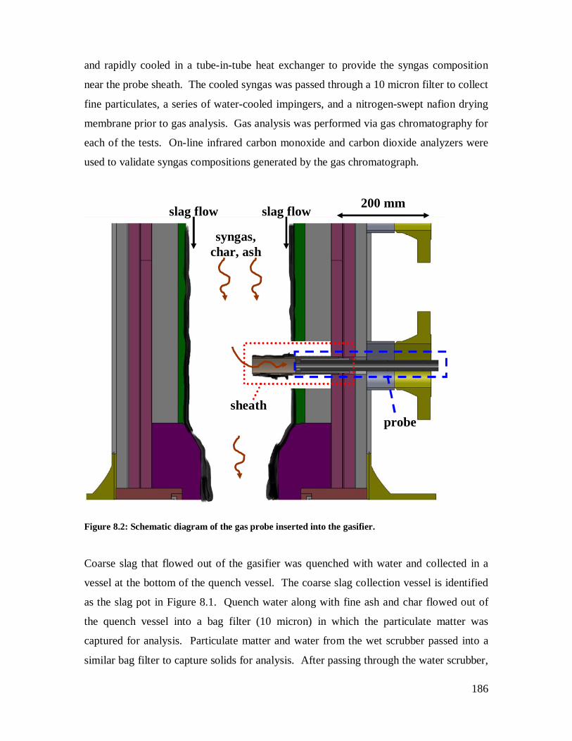
186

and rapidly cooled in a tube-in-tube heat exchanger to provide the syngas composition

near the probe sheath. The cooled syngas was passed through a 10 micron filter to collect

fine particulates, a series of water-cooled impingers, and a nitrogen-swept nafion drying

membrane prior to gas analysis. Gas analysis was performed via gas chromatography for

each of the tests. On-line infrared carbon monoxide and carbon dioxide analyzers were

used to validate syngas compositions generated by the gas chromatograph.

Figure 8.2: Schematic diagram of the gas probe inserted into the gasifier.

Coarse slag that flowed out of the gasifier was quenched with water and collected in a

vessel at the bottom of the quench vessel. The coarse slag collection vessel is identified

as the slag pot in Figure 8.1. Quench water along with fine ash and char flowed out of

the quench vessel into a bag filter (10 micron) in which the particulate matter was

captured for analysis. Particulate matter and water from the wet scrubber passed into a

similar bag filter to capture solids for analysis. After passing through the water scrubber,

syngas, char, ash

200 mm slag flow slag flow

sheath probe

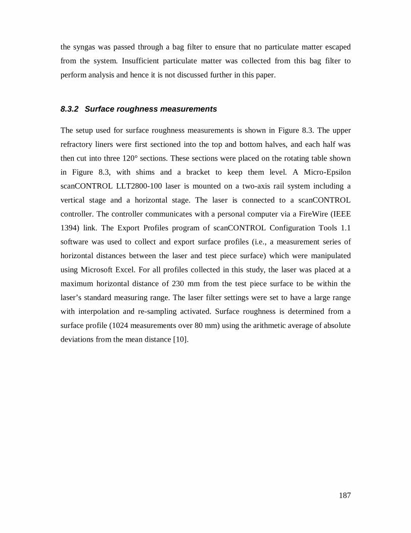
187

the syngas was passed through a bag filter to ensure that no particulate matter escaped

from the system. Insufficient particulate matter was collected from this bag filter to

perform analysis and hence it is not discussed further in this paper.

8.3.2 Surface roughness measurements

The setup used for surface roughness measurements is shown in Figure 8.3. The upper

refractory liners were first sectioned into the top and bottom halves, and each half was

then cut into three 120° sections. These sections were placed on the rotating table shown

in Figure 8.3, with shims and a bracket to keep them level. A Micro-Epsilon

scanCONTROL LLT2800-100 laser is mounted on a two-axis rail system including a

vertical stage and a horizontal stage. The laser is connected to a scanCONTROL

controller. The controller communicates with a personal computer via a FireWire (IEEE

1394) link. The Export Profiles program of scanCONTROL Configuration Tools 1.1

software was used to collect and export surface profiles (i.e., a measurement series of

horizontal distances between the laser and test piece surface) which were manipulated

using Microsoft Excel. For all profiles collected in this study, the laser was placed at a

maximum horizontal distance of 230 mm from the test piece surface to be within the

laser’s standard measuring range. The laser filter settings were set to have a large range

with interpolation and re-sampling activated. Surface roughness is determined from a

surface profile (1024 measurements over 80 mm) using the arithmetic average of absolute

deviations from the mean distance [10].

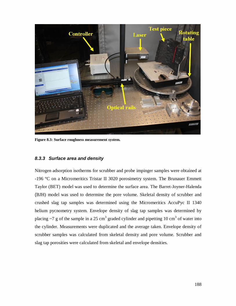
188

Figure 8.3: Surface roughness measurement system.

8.3.3 Surface area and density

Nitrogen adsorption isotherms for scrubber and probe impinger samples were obtained at

-196 °C on a Micromeritics Tristar II 3020 porosimetry system. The Brunauer Emmett

Taylor (BET) model was used to determine the surface area. The Barret-Joyner-Halenda

(BJH) model was used to determine the pore volume. Skeletal density of scrubber and

crushed slag tap samples was determined using the Micromeritics AccuPyc II 1340

helium pycnometry system. Envelope density of slag tap samples was determined by

placing ~7 g of the sample in a 25 cm3 graded cylinder and pipetting 10 cm3 of water into

the cylinder. Measurements were duplicated and the average taken. Envelope density of

scrubber samples was calculated from skeletal density and pore volume. Scrubber and

slag tap porosities were calculated from skeletal and envelope densities.

189

8.3.4 Other methods

ASTM D7582 was applied for determination of ash content in solid samples. ASTM

D5373 was applied for determination of carbon content in solid samples, except for probe

samples since the amount collected was insufficient for this procedure. Alternatively,

ASTM D5291 was applied for determination of carbon content in samples from the

probe. ASTM D4326 was applied to determine major and minor oxides content via X-ray

fluorescence (XRF).

Quantitative X-ray diffraction (XRD) analysis of the samples was performed over the

angular range of 7 to 80° (2θ). Each sample was mixed with an internal standard.

Integrated intensities for strong diffracting peaks of each phase were obtained using

JADE version 7.0 XRD processing software. Concentrations of the chemicals identified

in each sample were calculated using the reference intensity ratio (RIR) method.

Scanning electron microscopy with energy dispersive X-ray spectroscopy (SEM-EDX)

analysis was completed for cross-sections of the slag-covered refractory and solids from

the probe impingers and scrubber water. Samples were mounted with carbon tape on an

aluminum holder. A Hitachi 3400N VP-SEM with Oxford Instruments Si(Li) Pentafet

Plus X-Max 20 mm2 detector was used. X-ray acquisition was done with Oxford AZtec

Point and ID software. Quantification was done with the base Oxford factors.

57Fe Mössbauer spectroscopy measurements were conducted at room temperature using a

standard Mössbauer spectrometer operating in a sine mode and with a 57Co(Rh) gamma-

ray source. The spectrometer was calibrated with a 6.35-µm-thick α-Fe foil.

190


8.4.1 Description of pilot plant tests

Five gasification tests were conducted. Details for each are provided in Table 8.1. The

tests lasted 2-4 h. Injection rates, discharge rates, temperatures and dry syngas

compositions presented in Table 8.1 are averages for the final hour of operation. These

are representative of the quasi-steady state operating conditions during each test in terms

of feed rates and syngas composition, and are most representative of the conditions prior

to system quenching at the end of each test. The gasifier design allowed removal of the

upper refractory liner after each test. An alumina liner was used for tests T1 and T2. An

alumina-chromia (30 wt.% chromia) liner was used for tests T3-T5.

For each test, solid samples were collected from gas probe impingers, the slag tap, the

slag pot, the quench water discharge and the scrubber. The ash content, carbon content

and mass of the dried solids are given in Table 8.2. There was insufficient sample for

analysis from the scrubber for test T2, and from the probe for tests T1 and T5. Using the

results in Table 8.2 in conjunction with the total slurry mass consumed and composition,

ash and carbon mass balances were performed for each gasification test. Results of the

ash and carbon mass balances are presented in Tables 8.3 and 8.4, respectively. Note that

the mass of ash accumulated in the gasifier was calculated by difference. It was assumed

that accumulated ash in the gasifier has the same carbon content as ash at the slag tap.

The carbon in the syngas was calculated by difference and was used to calculate the total

mass of syngas produced. The carbon conversion and cold gas efficiency were calculated

for each test and are given in Table 8.1.

191

Table 8.1: Conditions for pilot-scale gasifier tests

Test name T1 T2 T3 T4 T5 Fuel F1 F1 F1 F3 F4

Upper refractory liner material alumina alumina alumina-chromia

alumina-chromia

alumina-chromia

Amount L2 per amount fuel (kg/kg) 0.000 0.000 0.000 0.042 0.099 Slurry moisture (wt.%) 58.0 56.0 59.5 54.6 52.1 Slurry used (kg) 200 156 197 257 158 Test duration (h) 2.46 2.62 2.85 3.36 2.05 Slurry injection rate (kg/h) 82.9 66.0 75.6 81.5 80.6 Oxygen injection rate (kg/h) 43.8 33.9 37.1 48.3 43.1 Quench water injection rate (kg/h) 302 214 172 350 327 Quench water discharge rate (kg/h) 367 291 241 389 369 TC1 temperature (°C) 1466 1593 1609 1554 1582 TC2 temperature (°C) 1413 1562 1441 1476 1501 TC3 temperature (°C) 1381 1422 1339 1440 1452 TC4 temperature (°C) 1285 1254 1253 1385 1371 Dry syngas composition

H2 (vol.%) 25.1 21.7 24.0 29.6 23.1 CO (vol.%) 28.0 20.9 24.5 41.9 25.0 CO2 (vol.%) 46.1 56.3 50.6 28.0 50.7

Carbon conversiona (%) 99.5 98.7 97.0 99.6 97.8 Cold gas efficiencyb (%) 44.1 33.7 38.8 61.9 39.3

a Based on carbon content of solids. b Based on higher heating values.

A very small amount of solids was entrained with the syngas to the scrubber. Most of the

solids were collected from the slag tap and slag pot. However, the majority of the solids

in tests T1 and T2 accumulated in the gasifier. Carbon conversion was 97.0% or greater

for every test. Most of the unconverted carbon was found in the slag pot. Cold gas

efficiencies varied from 33.7 to 61.9%. It should be noted that optimization of conversion

and efficiency was not the primary objective of the gasifier tests, but rather steady

gasification conditions for analysis of the inorganic matter were desired.

192

Table 8.2: Ash content, carbon content and mass of dried collected solids

Ash Carbon Mass Test Source (wt.%) (wt.%) (g)

T1 scrubber 20.0 71.9 19 T2 scrubber 3.2 85.2 7 T4 scrubber 77.0 20.0 95 T5 scrubber 18.1 73.8 9 T2 probe N/A 1.7 < 1 T3 probe N/A 24.7 < 1 T4 probe N/A 31.1 < 1 T1 quench discharge 91.2 9.0 146 T2 quench discharge 33.0 51.4 990 T3 quench discharge 53.5 37.6 447 T4 quench discharge 81.3 19.2 338 T5 quench discharge 78.1 18.8 165 T1 slag tap 98.1 1.7 3288 T2 slag tap 100.0 0.1 3363 T3 slag tap 100.0 0.0 2901 T4 slag tap 100.0 0.0 5775 T5 slag tap 100.0 0.0 2264 T1 slag pot 96.3 3.5 2994 T2 slag pot 66.1 26.2 113 T3 slag pot 83.8 14.1 9282 T4 slag pot 96.3 3.3 8144 T5 slag pot 94.7 4.4 18940 T1 slag pot (chunks) 100.0 0.0 N/A T2 slag pot (chunks) 98.3 1.3 N/A T3 slag pot (chunks) 99.1 0.7 N/A T4 slag pot (chunks) 100.0 0.0 N/A T5 slag pot (chunks) 100.0 0.0 N/A T1 slag pot (sheets) 100.0 0.0 N/A T5 slag pot (sheets) 99.8 0.2 N/A

193

Table 8.3: Ash mass balance

T1 T2 T3 T4 T5

Total in (g) 12372 10134 11778 14816 22009 Slag tap (g) 3241 3364 2901 5775 2263 Slag pot (g) 2884 75 7782 7847 17944

Quench discharge (g) 133 327 239 275 129 Scrubber (g) 4 0 0 73 2

Accumulated in gasifier (g) 6110 6369 856 845 1672

Table 8.4: Carbon mass balance

T1 T2 T3 T4 T5

Total in (g) 51796 42427 49308 78961 38970 Slag tap (g) 44 2 0 0 0 Slag pot (g) 105 30 1306 268 834

Quench discharge (g) 13 509 168 65 31 Scrubber (g) 13 6 0 19 7

Accumulated in gasifier (g) 104 6 0 0 0 Syngas (g) 51516 41874 47833 78608 38099

8.4.2 Char and fly ash

Solid samples collected from the gas probe impingers are representative of char and fly

ash ~150 mm above the slag tap. Samples collected from the scrubber are representative

of char and fly ash which were entrained out of the reactor by syngas. Ash content,

carbon content, as well as mass of samples collected from the scrubber and probe are

given in Table 8.2. The probe samples contain 2-31 wt.% carbon. Scrubber samples

contain 20-85 wt.% carbon. Ash compositions of the solid samples, on a major and minor

oxides basis, are provided in Table 8.5. Fuel ash compositions are included in this table

for comparison. Quantitative XRD analyses of the solid samples are provided in Table

8.6. Masses of probe samples were insufficient for the characterization in Tables 8.5 and

8.6. Compared to the fuel ashes, scrubber samples from tests T1 and T2 are enriched in

194

Table 8.5: Major and minor oxides in ash of collected solid samples (part 1 of 2)

SiO2 Al2O3 Fe2O3 TiO2 P2O5 CaO MgO SO3 Na2O K2O Cr2O3 Test Source (wt.%) (wt.%) (wt.%) (wt.%) (wt.%) (wt.%) (wt.%) (wt.%) (wt.%) (wt.%) (wt.%)

T1 scrubber 50.3 22.1 6.7 0.7 0.3 5.5 0.6 4.4 5.1 1.7 1.1 T2 scrubber 49.8 22.0 14.4 0.0 0.0 7.9 0.0 0.0 0.0 0.7 2.9 T4 scrubber 45.2 19.3 4.9 0.7 0.8 23.6 1.7 0.9 0.6 1.1 0.1 T5 scrubber 43.4 20.6 7.6 1.0 0.8 15.7 0.7 7.0 0.0 1.2 1.2 T1 quench discharge 52.8 22.3 4.3 0.8 0.2 8.0 2.0 0.5 6.4 1.6 0.2 T2 quench discharge 51.8 20.7 5.5 0.7 0.2 9.6 1.4 5.0 2.9 1.2 0.1 T3 quench discharge 48.4 25.7 4.9 0.7 0.2 9.6 2.3 1.7 4.4 1.2 0.2 T4 quench discharge 48.4 18.2 5.0 0.6 0.8 22.1 1.5 0.6 0.7 1.5 0.1 T5 quench discharge 54.1 17.0 4.4 0.5 0.1 18.3 1.0 0.5 1.3 2.1 0.1 T1 slag tap 51.4 21.5 5.5 0.8 0.2 11.0 2.4 0.0 5.0 1.1 0.1 T2 slag tap 49.5 24.3 5.5 0.8 0.2 9.8 2.4 0.0 5.0 1.1 0.5 T3 slag tap 48.5 22.4 5.8 0.8 0.2 10.4 2.7 0.0 5.1 1.1 2.1 T4 slag tap 46.8 19.2 5.8 0.5 0.4 21.5 1.8 0.0 0.9 1.0 1.5 T5 slag tap 49.0 20.4 5.0 0.5 0.1 18.1 1.4 0.0 1.5 1.2 2.4

194

195

Table 8.5: Major and minor oxides in ash of collected solid samples (part 2 of 2)

SiO2 Al2O3 Fe2O3 TiO2 P2O5 CaO MgO SO3 Na2O K2O Cr2O3 Test Source (wt.%) (wt.%) (wt.%) (wt.%) (wt.%) (wt.%) (wt.%) (wt.%) (wt.%) (wt.%) (wt.%)

T1 slag pot 51.9 20.5 5.6 0.8 0.2 11.0 2.6 0.0 5.1 1.2 0.1 T2 slag pot 52.0 21.0 5.7 0.8 0.2 10.3 2.3 0.8 4.5 1.2 0.3 T3 slag pot 48.4 23.7 5.4 0.7 0.2 10.5 2.3 0.2 4.8 1.1 1.8 T4 slag pot 45.2 22.0 5.6 0.5 0.4 20.2 1.7 0.2 1.0 1.1 1.6 T5 slag pot 53.6 16.6 4.9 0.5 0.1 19.6 1.2 0.0 1.3 1.5 0.4 T1 slag pot (chunks) 51.9 20.8 5.5 0.8 0.2 10.8 2.7 0.0 5.2 1.1 0.1 T2 slag pot (chunks) 51.8 21.5 5.8 0.8 0.2 10.2 2.5 0.0 5.0 1.1 0.2 T3 slag pot (chunks) 50.5 21.6 5.4 0.8 0.2 10.9 2.6 0.0 5.3 1.1 0.6 T4 slag pot (chunks) 48.7 19.2 6.0 0.6 0.3 17.8 2.1 0.0 2.3 1.1 1.3 T5 slag pot (chunks) 54.5 15.9 4.8 0.5 0.1 19.8 1.2 0.0 1.3 1.5 0.2 T1 slag pot (sheets) 51.5 20.7 5.5 0.8 0.2 11.2 2.5 0.0 5.3 1.2 0.1 T5 slag pot (sheets) 21.1 51.2 3.0 0.2 0.1 7.9 1.0 0.0 0.7 0.4 14.2 T1 slag pot (filaments) 52.5 20.6 5.4 0.8 0.2 11.2 2.2 0.0 5.0 1.2 0.0 T5 slag pot (filaments) 54.8 15.7 4.6 0.5 0.0 19.9 1.1 0.0 1.3 1.5 0.1

T1-T3 F1 fuel 38.0 16.3 6.3 0.7 0.4 13.6 2.7 14.3 6.0 0.3 0.0 T4 F3:L2 fuel 45.6 15.2 5.6 0.5 0.5 25.7 1.6 3.8 0.3 1.1 0.0 T5 F4:l2 fuel 48.4 16.6 3.9 0.6 0.0 21.5 1.4 4.1 1.9 1.5 0.0

195

196

Table 8.6: Quantitative XRD analyses for solid samples (values reported as wt.%)

scrubber slag tap slag pot slag pot, filaments

T1 T2 T4 T5 T1 T2 T3 T4 T5 T1 T2 T3 T4 T5 T1 T5

CaAl2Si2O8 0.0 0.0 0.0 0.0 0.0 0.0 0.0 0.0 0.0 0.0 0.0 2.7 0.0 0.0 0.0 0.0 (Ca,Na)(Al,Si)2Si2O8 0.0 0.0 0.0 0.0 0.0 0.0 0.0 0.0 0.0 0.0 0.8 0.0 0.0 0.0 0.0 0.0

(Mg,Fe,Ti,Al)(Ca,Na,Mg,) (Si,Al)2O6

0.0 0.0 0.0 0.0 6.1 16.7 8.4 0.0 0.0 0.0 0.0 0.0 0.0 0.0 0.0 0.0

Ca(CO3) 2.3 0.9 0.0 1.6 0.6 0.0 0.0 0.0 0.0 0.0 0.0 0.0 8.1 0.2 0.0 0.0 Ca(SO4)(H2O)0.6 5.2 0.6 0.0 4.3 0.0 0.0 0.0 0.0 0.0 0.0 0.0 0.0 0.0 0.0 0.0 0.0

FeCr2O4 0.0 0.0 0.0 0.0 0.0 1.9 1.8 1.7 3.2 0.0 0.0 0.0 0.0 0.0 0.0 0.0 CrO2 0.0 0.0 0.0 0.0 0.0 0.0 0.0 0.0 0.0 0.0 0.0 0.9 0.0 0.0 0.0 0.0 Al2O3 0.0 0.0 0.0 0.0 0.0 0.0 0.0 0.0 0.0 0.0 0.0 5.3 8.0 0.0 0.0 0.0 Cr2O3 0.0 0.0 0.0 0.0 0.0 0.0 0.0 0.0 0.0 0.0 0.0 0.0 4.0 0.0 0.0 0.0 Fe2O3 0.0 0.0 0.0 0.0 0.0 0.4 0.0 0.0 0.0 0.0 0.0 0.0 0.8 0.0 0.0 0.0

(Fe0.324Si0.676) (Fe0.963Si0.037)2O4

0.6 0.0 0.0 0.0 0.0 0.0 7.1 5.7 2.5 0.0 0.0 0.0 0.0 0.0 0.0 0.0

Ca0.65Na0.32 (Al1.62Si2.38O8) 0.0 0.0 0.0 0.0 14.3 69.8 64.1 73.6 64.3 0.0 0.0 4.8 0.0 0.0 0.0 0.0 Mg3Si2O5(OH)4 0.0 0.0 0.0 0.0 0.0 0.0 0.0 0.0 0.0 0.0 0.7 0.0 0.0 0.0 0.0 0.0

MgAlCrO4 0.0 0.0 0.0 0.0 0.0 0.0 0.0 0.0 0.0 0.0 0.0 0.0 0.0 0.0 0.0 0.0 KAl(Mg0.2Al0.8)

(Al0.42Si3.58)O10(OH)2 0.0 0.0 0.0 0.0 0.0 0.0 0.0 0.0 0.0 0.0 0.9 0.0 0.0 0.0 0.0 0.0

Na6K1.2Al7.2Si8.8O32 0.0 0.0 0.0 0.0 0.0 7.0 8.6 0.0 7.3 0.0 0.0 0.0 0.0 0.0 0.0 0.0 CaAl2Si2O8 0.0 0.0 0.0 0.0 0.0 0.0 0.0 0.0 0.0 0.0 0.0 0.0 0.5 0.0 0.0 0.0

SiO2 4.6 1.3 6.3 4.1 0.0 0.0 0.0 0.0 0.0 3.4 2.6 6.0 5.7 0.6 0.0 0.0 TiO2 0.0 0.0 0.0 0.0 0.0 0.0 0.0 0.0 0.0 0.1 0.0 0.0 0.6 0.1 0.0 0.0

Na1.71Al0.43(PO4) 0.0 0.0 0.0 0.0 0.0 0.0 0.0 0.0 0.0 0.0 0.0 1.8 0.0 0.0 0.0 0.0 Amorphous 87.2 97.2 93.7 90.1 79.0 4.1 10.1 19.0 22.7 96.5 95.0 78.5 72.5 99.1 100.0 100.0

196

197

SiO2 and Al2O3. These samples are also depleted in CaO. Scrubber samples from tests T4

and T5 have ash compositions which are closer to the feed ash composition. However, all

scrubber samples contain Cr2O3 which was not present in the feed ashes. The Cr2O3 must

have originated from the gasifier refractory. The inorganic matter in the scrubber samples

is 87-97% amorphous.

Table 8.7 provides surface area, skeletal density, envelope density and porosity of the

scrubber samples. The scrubber sample from test T2 only has skeletal density provided

since attempts to obtain nitrogen adsorption isotherms failed. Surface area of test T1 and

T4 scrubber samples are approximately three times greater than the surface area of the

test T5 scrubber sample. The T5 scrubber sample also has much lower porosity than the

other scrubber samples, which is expected with lower surface area. It may be that this

sample has less char, denser char and/or more plugging of pores by inorganic matter

compared to the other scrubber samples. The T4 scrubber sample has the highest skeletal

and envelope densities. This is expected since it has higher ash content than the other

scrubber samples and inorganic matter is generally denser than organic matter. SEM

images of the scrubber and probe samples are shown in Figure 8.4. Many features

observed in these and additional SEM images were analysed by EDX. Annotations are

added in Figure 8.4 to highlight some of these features. In the SEM images, char particles

are darker than inorganic matter. EDX analyses of char surfaces without inorganic matter

indicate a carbon content exceeding 80 wt.%. The structure of the char affects

coalescence and expulsion of included particles of inorganic matter [11,12]. Yu et al. [13]

present an equation which correlates the number percentage of char with more than 80%

porosity ( cN ) to pressure ( P in MPa) and the reactive maceral content of coal ( rM in

%):

3753.06 rc MPN

198

Table 8.7: Surface area, skeletal density, envelope density and porosity of solid samples

Surface area Skeletal density Envelope density Porosity Test Source (m2/g) (g/cm3) (g/cm3)

T1 scrubber 31.27 1.78 1.35 0.239 T2 scrubber N/A 1.43 N/A N/A T4 scrubber 34.63 2.45 2.02 0.172 T5 scrubber 10.53 1.64 1.57 0.041 T2 probe 15.54 N/A N/A N/A T3 probe 11.37 N/A N/A N/A T4 probe 12.23 N/A N/A N/A T1 tap N/A 2.64 2.1 0.21 T2 tap N/A 2.82 2.0 0.28 T3 tap N/A 2.89 2.1 0.26 T4 tap N/A 2.67 2.1 0.22 T5 tap N/A 2.85 2.2 0.22

198

199

Figure 8.4: SEM images comparing scrubber and probe impinger samples: (a) T1 scrubber, (b) T2 scrubber, (c) T4 scrubber, (d) T5 scrubber, (e) T1

impinger, (f) T3 impinger and (g) T4 impinger. The scale in the (a) image applies to all images. 199

200

With the maceral content of the fuels obtained in the fuel characterization study [4], 88-

92% of char particles are expected to have a porosity exceeding 80%. From SEM

analysis of the scrubber and impinger samples, the proportion of highly porous char

seems to be much lower than the predicted proportions. This may be due to higher

conversion of porous char and differences in particle trajectories or sticking.

In all scrubber samples, most inorganic matter is spherical. Considering the low

crystallinity of the ash in these samples (3-13%) and the high crystallinity of the feed

ashes (71-95%), it appears that the majority of the inorganic matter melted in the gasifier

and formed spheres due to surface energy minimization. Most of the inorganic matter on

the char particles is spherical, indicating that the liquid slag on the char is non-wetting.

The melting of inorganic matter and low wetting of char confirm assumptions made in

ash particle formation models [11,12]. The compositions of the slag spheres are quite

variable, but for the most part resemble the fuel ash composition. Many of the scrubber

and probe samples contain separate non-spherical phases rich in chrome and iron. This

indicates the chrome from the refractory material reacted with iron in the slag and

spalling and/or erosion occurred. The strands observed in the probe samples are from the

filters used in the probe impingers. Except for samples from test T4, the probe samples

seem to contain less char than their scrubber counterparts. This result was validated by

the measured carbon content of the samples as presented in Table 8.2. The discrepancies

of char-to-ash ratios in the probe and scrubber samples may be caused by differences in

particle trajectories and/or sticking to surfaces.

The carbon content of the scrubber samples is greater than the average carbon content of

all solid samples combined. This suggests that compared to the proportion of fly ash

particles collected from the scrubber, a greater proportion of char particles are entrained

with the syngas to the scrubber rather than captured by water in the slag pot or quench

discharge. For particles to make it to the scrubber, they must flow down with the gas

phase through the slag tap and into the quench vessel, and then be brought up with the

gas to the syngas outlet instead of submerging into the water in the quench vessel.

According to Stokes’s law, it is easiest for smaller and lower density particles to achieve

201

this feat. Char particles have lower density than fly ash particles and are therefore likelier

to be entrained. There are several possible causes to explain why a greater amount of ash

made it to the scrubber during test T4. The fly ash could have been smaller or had a lower

density. Also, the gas velocity may have been greater. Alternatively, the fly ash particles

may have had a lower wall impaction/sticking rate with the surfaces in the gasifier during

test T4.

8.4.3 Slag from the slag tap, slag pot and quench water discharge

Major and minor oxides compositions of samples collected at the slag tap, in the slag pot

and in the quench water discharge are provided in Table 8.5. All slags from a given test

have similar major and minor oxides compositions. Crystalline phase content of samples

collected at the slag tap and in the slag pot is provided in Table 8.6. Skeletal density,

envelope density and porosity of slag tap samples are provided in Table 8.7.

Together, SO3 and Na2O represent 4-20 wt.% of the feed ashes. However, they are

expected to partially or fully devolatilize in the gasifier. Compared to the feed ashes, the

content of SO3 in the slag tap, slag pot and quench water discharge samples decreased by

65-100%. The content of Na2O decreased by 15-52% in all these samples except test T4

samples which have increases of 123-203%, and the quench water discharge sample from

test T3 which has an increase of 7%. The increase in sodium content for test T4 slags is

likely due to contamination from slag accumulated in the gasifier during previous tests.

Nonetheless, the amount of Na2O in these slags remains small (≤ 1 wt.%). Excluding the

SO3 and Na2O loss, most slag samples are enriched in SiO2, enriched in Al2O3 and

depleted in CaO. These changes may be caused by interactions with the gasifier

refractory and slag accumulated in the gasifier during previous tests.

Ca0.65Na0.32(Al1.62Si2.38O8) dominates the crystalline portion of the slag tap slags. This

compound has a composition which is similar to the slag major and minor oxides

compositions and has a melting temperature of 1400 °C [14]. The slag tap slags also

contained up to 3.2 wt.% FeCr2O4, which has a melting temperature of 1670 °C [15]. The

202

FeCr2O4 in the slag at the slag tap is likely a result of iron in slag reacting with the

refractory and forming FeCr2O4 which then detaches from the refractory, or chromium

from the refractory dissolving in slag and then precipitating as FeCr2O4.

The slag pot samples have much higher amorphous content than the slag tap samples

(Table 8.6). The higher amorphous content of the slag in the slag pot suggests that most

of the slag flowed down from the slag tap and was rapidly quenched. Solids with

different shapes were discovered in the slag pot, as can be seen in Figure 8.5. Slag chunks

were found in all the slag pot samples. Their major and minor oxides composition is

roughly the same as the slag pot slag composition (Table 8.5). However, they contain

much less carbon (Table 8.2). These chunks are slag which flowed from the slag tap and

into the quench vessel. Filaments were found in slag pot samples from tests T1, T3 and

T5. These are mostly translucent and green. They are completely amorphous (Table 8.6)

and their major and minor oxides composition is roughly the same as the slag pot slag

composition (Table 8.5), although they contain almost no carbon (Table 8.2). Slag sheets

were found in slag pot samples from tests T1 and T5. They contain very little carbon

(Table 8.2). Slag sheets from test T1 resembled the slag pot slag composition in terms of

major and minor oxides (Table 8.5). However, sheets from test T5 are highly enriched in

Al2O3 and Cr2O3. The sheets from test T1 may be cracked pieces of slag. Sheets from test

T5 seem to be pieces of slag with refractory.

The carbon content of slag samples from the quench discharge water (9-51%) is higher

than the carbon content of slag from the slag pot (3-26%). Hence, the proportion of char

that goes in the quench water discharge (as opposed to remaining in the slag pot) is

greater than the proportion of ash which goes in the quench water discharge. This is

expected since the higher density slag can rapidly sink down in the water in the slag pot,

while lighter char tends to stay on top or does not sink as quickly. The water which is

removed from the top of the slag pot can therefore entrain a higher fraction of the char in

the higher slag pot water as it is discharged. The quench water does contain a significant

portion of the unconverted char particles (Table 8.4). Nonetheless, for four of the five

tests, more carbon was present in the slag pot.

203

Figure 8.5: Slag collected from the slag pot after test T5 (a) and classified according to shape: (b) slag

chunks, (c) slag filaments and (d) slag sheets.

Beyond the atomic composition of slag, there is much interest in knowing the oxidation

state of slag iron in the gasifier since it can affect slag flow and interaction with the

refractory. The oxidation state of the iron in the slag will depend on many factors such as

temperature, gas phase composition and slag composition [16]. Assumptions on the

oxidation state can be made based on temperature and oxygen partial pressure in the

gasifier, but whether gas-slag equilibrium is achieved remains unclear. 57Fe Mössbauer

spectroscopy measurements indicate that virtually all the iron atoms in the slag collected

from the slag pot after tests T1-T5 are in the divalent oxidation state. This suggests that

iron in slag flowing through the slag tap is in the divalent oxidation state before reaching

the quench vessel and experiencing rapid quenching.

a) b)

c) d)

204

8.4.4 Slag layer on refractory

The following equation to calculate the thickness of slag ( ) assumes a steady-state

falling film of slag on a vertical surface with laminar flow, negligible rippling at the slag-

gas interface, no slip at the wall, slag entrainment is entirely caused by gravity (i.e., there

is no shear stress at the slag gas interface), all ash entering the gasifier sticks to the wall,

the film thickness is much smaller than the reactor diameter, and the slag properties are

constant:

31

23

gCm

where m is the injection rate of ash which is calculated from slurry used, test duration,

slurry moisture content and fuel ash content. is the density of the slag which is taken

as the envelope density of slag at the slag tap. g is acceleration due to gravity. C is the

circumference of the refractory liner. is the slag viscosity. For slag thickness

predictions with the upper refractory liners, the TC1 temperature is assumed. For slag

thickness predictions with the probe sheaths, the TC4 temperature is assumed. For each

sheath and liner, the slag thickness calculations were first completed by predicting the

slag viscosity from measured values in the fuel characterization study [4]. This assumes

the feed ash composition applies. The thickness calculations were then repeated with the

assumption that the slag pot ash composition applies. In this case, the slag viscosity

model used for prediction was selected using the method presented by Duchesne et al.

[17]. Ash injection rates, predicted slag viscosities and predicted slag layer thicknesses

are given in Table 8.8. The slag viscosities predicted with the slag pot slag composition

tend to be higher than those predicted with the feed ash composition. In some cases, the

former is more than five times greater than the latter. Still, the two thicknesses never

differ by more than 1.5 mm.

205

The slag flow in the gasifier can be considered laminar if the Reynolds number ( ReN ) is

less than 1200 and negligible rippling will occur when it is lower than 20 [18,19]. The

Reynolds number can be obtained from:

2

32

Re 34

gN

The calculated Reynolds numbers for slag flowing on the upper refractory liner and on

the probe sheath are given in Table 8.8. Values for each predicted slag viscosity are

given. The Reynolds numbers are very small and the assumption of laminar flow with

negligible rippling is applicable. In all cases, with all other parameters constant, the slag

thickness would have to be at least ten times greater for non-negligible rippling to occur.

Slag thicknesses on the liners and probe sheaths were measured using Vernier calipers.

For the liners, averages of ten measurements with standard deviations are provided in

Table 8.8. For the probe sheath, the maximum thickness is provided in Table 8.8.

Figure 8.6 shows photographs of upper refractory liners collected after each test. The

measured slag surface roughness values are shown in Figure 8.7. Liners from tests T1 and

T2 have smoother slag surfaces than the liners from tests T3-T5. Slag features on liners

from tests T1 and T2 are less than 0.5 mm thick. Slag features on liners from tests T3-T5

are up to 12 mm thick, but for the most part are much thinner. The predicted thicknesses

for liners from tests T1 and T2 are greater than what is observed experimentally. The

predicted thicknesses for liners from tests T3-T5 are smaller than what is observed. The

liner from test T1 presents some slag rivulets which are 3-50 mm in width and less than

0.5 mm thick. Some rivulets travelled the entire length of the liner. T2 also presents some

slag rivulets, however they are less numerous than for the liner from test T1. They are 3-

20 mm wide, 10-200 mm long and less than 0.5 mm thick. Most of the slag on the T2

liner is present as spots with diameters ranging from 1 to 80 mm. The larger spots are

mostly near seams, cracks and holes in the liner. The slag layers on liners from tests T3-

T5 are rough and bubbly. Bumps can protrude up to 35 mm. Some cavities are as deep as

20 mm. Gas bubbles may have been formed by decomposition or devolatilization of slag

206

components. Reaction with the refractory material may have prompted bubble formation

as well. Another hypothesis is that gas trapped in the refractory pores escapes as bubbles

while the slag penetrates the refractory material. Clearly, assumptions made in the above

slag thickness model do not represent reality and the formation of rivulets and bubbles

warrants future studies.

Table 8.8: Ash injection rates and slag layer properties

Test T1 T2 T3 T4 T5 Ash injection rate (kg/h) 5.0 3.9 4.1 4.4 10.7 At upper liner

Viscositya (Pa·s) 3.9 2.1 1.9 1.7 1.9 Viscosityb (Pa·s) 12.6 4.6 3.1 1.4 2.8 Model slag thicknessa (mm) 0.8 0.6 0.6 0.6 0.8 Model slag thicknessb (mm) 1.2 0.8 0.7 0.6 0.9 Measured thicknessc (mm) <0.5 <0.5 2.7 (1.2) 3.0 (0.6) 4.2 (3.5) Reynolds numbera 0.0018 0.0026 0.0038 0.0046 0.0100 Reynolds numberb 0.0006 0.0012 0.0024 0.0056 0.0068

At probe sheath Viscositya (Pa·s) 16.9 27.4 27.8 4.6 10.9 Viscosityb (Pa·s) 124 240 173 6.9 19.8 Model slag thicknessa (mm) 1.3 1.4 1.5 0.9 1.5 Model slag thicknessb (mm) 2.5 2.9 2.8 1.0 1.8 Measured thicknessd (mm) 19.0 4.0 <0.5 4 14.0 Reynolds numbera 0.00042 0.00020 0.00026 0.00169 0.00174 Reynolds numberb 0.00006 0.00002 0.00004 0.00113 0.00096

a assuming feed ash composition b assuming slag pot slag composition c standard deviation is in brackets d maximum thickness on sheath

207

Figure 8.6: Photos of liners (a-e) from tests T1-T5, respectively.

a)

b)

c)

d)

e)

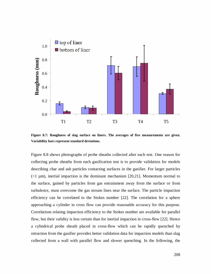
208

0.0

0.2

0.4

0.6

0.8

1.0

T1 T2 T3 T4 T5

Rou

ghne

ss (m

m)

top of linerbottom of liner

Figure 8.7: Roughness of slag surface on liners. The averages of five measurements are given.

Variability bars represent standard deviations.

Figure 8.8 shows photographs of probe sheaths collected after each test. One reason for

collecting probe sheaths from each gasification test is to provide validation for models

describing char and ash particles contacting surfaces in the gasifier. For larger particles

(>1 µm), inertial impaction is the dominant mechanism [20,21]. Momentum normal to

the surface, gained by particles from gas entrainment away from the surface or from

turbulence, must overcome the gas stream lines near the surface. The particle impaction

efficiency can be correlated to the Stokes number [22]. The correlation for a sphere

approaching a cylinder in cross flow can provide reasonable accuracy for this purpose.

Correlations relating impaction efficiency to the Stokes number are available for parallel

flow, but their validity is less certain than for inertial impaction in cross-flow [22]. Hence

a cylindrical probe sheath placed in cross-flow which can be rapidly quenched by

retraction from the gasifier provides better validation data for impaction models than slag

collected from a wall with parallel flow and slower quenching. In the following, the

209

convention used refers to the left of the probe sheath as the end that is in the gasifier. The

top corresponds to the top of the sheath as it was placed in the gasifier. All probe sheaths

are made of alumina, except for the sheath used in test T3 which is made of silicon

carbide. The probe sheath from test T1 cracked at 70 mm from the left end. Its entire top

is covered in slag which is typically less than 1 mm thick. Near where it cracked, slag is

up to 5 mm thick. The section of the sheath on the right that did not extend into the

gasifier can be distinguished as it does not have slag at the bottom. The left section which

was extended past the gasifier inner refractory has dripping slag, up to 19 mm thick. As

for the probe sheath from test T2, a piece broke off the top left. The entire top and left

side are covered in slag, generally less than 0.5 mm thick. The top left has areas with

thicker slag, but still less than 1 mm thick. The left bottom has slag which is up to 4 mm

thick. The bottom of the right section which did not extend into the gasifier is bare. For

the silicon carbide sheath collected from test T3, slag on its left side was knocked off as it

was removed from the gasifier. Some slag remained on the top right side. The built-up

slag thickness is less than 0.5 mm. Probe sheaths from tests T4 and T5 both had some

slag flake off the top left sections. The sheath from test T5 has more slag on it,

particularly on the top section aligned with the inner gasifier refractory. The measured

maximum thicknesses on the probe sheaths are compared to predicted values in Table

8.8. For all tests except T3, the predicted thicknesses are smaller than the maximum

measured thickness. Greater predicted thicknesses do not correspond to greater measured

maximum thicknesses. The slag thickness model is a poor representation of the slag layer

on the sheaths. A better model for slag flow on the sheaths would likely consider

interfacial tension. For example, less slag may have accumulated on the silicon carbide

sheath than the alumina sheath due to poorer sticking of char/ash/slag particles during

impaction on silicon carbide. Sticking is a function of the gas-slag, gas-refractory and

slag-refractory interfacial tensions [23]. Also, the bare silicon carbide sheath is smoother

than the bare alumina sheaths. Generally, wetting on rough surfaces is greater than on

smooth surface when the contact angle between the liquid and solid is less than 90° [10].

210

Figure 8.8: Photos of probe sheaths (a-e) from tests T1-T5, respectively.

The section on top of sheaths with thicker slag was aligned with the wall during gasifier

testing. This suggests slag flowed down from the refractory and onto the sheaths. Another

possible cause of the thicker slag would be higher char and fly ash particle density in the

gas phase near the wall, leading to increased impaction on the sheath in this area. This

can occur if particle sticking on the refractory is inhibited. Such is the case if there is

extensive coverage of char on the surface of slag flowing down the refractory [24,25].

b)

c)

d)

e)

180 mm

211

8.4.5 Slag-refractory interface

Pieces of slag-covered refractory near the mid-section of the upper refractory liner were

cut and cross-sections were used for SEM-EDX analysis. Temperature during gasifier

operation at the slag surface of these sections was assumed to be near the TC1

temperature given in Table 8.1. Figure 8.9 shows silicon, aluminum and calcium

elemental maps at the slag-refractory interface for tests T1 and T2. The interface between

the slag and alumina is clearly seen since little slag penetrated the alumina which has

high aluminum and low silicon concentrations. Spalling/eroding of alumina is seen in

Figure 8.9. SEM-EDX results for the slag near the alumina refractory indicate a 73% and

88% increase of atomic aluminum content for tests T1 and T2, respectively. The

distribution of elements in the slag suggests most of the slag has formed crystal

plagioclase with a small portion of amorphous slag surrounding the crystals. It is not

clear whether these crystals were present during the test or only formed upon shutdown

and cooling of the gasifier system. SEM images indicate that the slag layer thickness

varies but is typically 0.2 mm thick.

Percentages of slag penetration into the refractory were calculated as follows. The atomic

composition of a given refractory section was calculated by averaging the results of a

minimum of 20 SEM-EDX spectra. An estimated atomic composition of this section was

then expressed as a weighted average atomic composition combining the test’s feed ash

composition and the slag-free refractory composition. The sum of squared differences

between the components in this weighted average and the SEM-EDX spectra average was

minimized by allowing the weight of the feed ash and slag-free refractory to vary from 0

to 1, with their sum equal to 1. The weight of the feed ash is the slag penetration fraction.

At a depth of 0 to 150 µm into the refractory, in reference to the slag-refractory interface,

samples from tests T1 and T2 have 3.5% and 5.4% slag penetration, respectively.

212

Figure 8.9: Silicon (Si), aluminum (Al) and calcium (Ca) elemental maps produced by SEM-EDX of slag-refractory cross-sections for tests T1 (a) and

T2 (b). The scale in the left image applies to the centre and right images.

100 µm

500 µm

a) Si ia) Ali a) Ca

b) Si ib) Ali b) Ca

212

213

Elemental maps for tests T3-T5 are not shown since it is difficult to locate a slag-

refractory interface. Slag penetration was calculated as a function of depth into the

refractory, in reference to the slag-covered surface. Results are given in Figure 8.10. Slag

penetrated approximately 20, 12 and 8 mm for tests T3, T4 and T5 respectively. Even in

the first millimeter of depth, where the sample looks like dark slag, the purity of the slag

is less than 80%. The slag percentage does not continuously decrease with depth. This

can be due to the presence of pores, cracks in the refractory, or due to the heterogeneous

composition of the refractory. Slag penetration is a major cause of refractory wear.

Penetration depth is, among other factors, a function of temperature, slag viscosity, slag-

refractory interfacial tension, slag-refractory reactions, refractory porosity and exposure

duration [26]. The viscosity of slag on the liners should be similar for tests T3-T5, as

indicated in Table 8.8. However, temperature, exposure time and slag compositions vary

between tests and it is difficult to isolate which parameters had the greatest effect on

penetration.

0.0

0.1

0.2

0.3

0.4

0.5

0.6

0.7

0.8

0 5 10 15 20

Depth in refractory (mm)

Slag

frac

tion

T3T4T5

Figure 8.10: Slag penetration in alumina-chromia refractory.

214

8.5 Conclusion

Five tests have been completed with CanmetENERGY’s pilot-scale gasifier. The first

three tests were with fuel F1, the fourth with F3:L2 and the fifth with F4:L2. The gasifier

configuration allowed replacement of the upper refractory liner after each test. Alumina

liners were used for the first two tests. Alumina-chromia liners were used for subsequent

tests. Carbon conversions and cold gas efficiencies for the tests were within 97.0-99.6%

and 33.7-61.9%, respectively. Samples collected from the gas probe impingers and

scrubber have relatively high carbon concentrations, but most of the unconverted carbon

was collected in slag from the slag pot and quench water discharge. Char and fly ash

samples indicate that most of the inorganic matter melted and formed spheres, regardless

of whether it was associated to char or not. Amorphous slag ran down the slag tap and

dripped into the slag pot. Some slag accumulated near the slag tap and crystallized. Slag

collected from the gasifier was affected by devolatilization and interaction with the

gasifier refractory. This can significantly impact slag properties such as viscosity. Signs

of spalling and/or erosion were detected by SEM-EDX analysis of the slag-refractory

interface from the first two tests. The chromium-rich particles found in scrubber, probe

impinger and slag pot samples are other signs of spalling/erosion. Slag accumulated on

the alumina liners is thin (~0.2 mm) and formed rivulets and spots. The slag is enriched

in aluminum and penetration into the alumina refractory was 3.5-5.4% at a depth of 0-150

µm. Slag layers on the alumina-chromia liners are rough and bubbly. For these liners, the

slag-refractory interface is difficult to distinguish, but slag thickness was estimated at 2.7-

4.2 mm. Slag penetrated 8-20 mm into the alumina-chromia liners. Measured slag

thicknesses were compared to predicted slag thicknesses. The slag thickness model used

should be improved by considering interfacial tensions, deviation from the vertical wall

assumption and non-constant slag properties.

215


Jeffery Slater and Ryan Burchat of CanmetENERGY were invaluable for the operation

and maintenance of the pilot-scale gasifier. Part of this research has been funded by the

Natural Sciences and Engineering Research Council of Canada (NSERC) and the

Canadian Federal Program for Energy Research and Development (PERD).

8.7 References

[1] Higman C, van der Burgt M, (Eds.). Gasification, 2nd ed. Gulf Professional


[2] National Energy Technology Laboratory Gasifipedia, Available from:

http://www.netl.doe.gov/technologies/coalpower/gasification/gasifipedia/TOC.html,

2012.




[4] Duchesne MA, Hall AD, Hughes RW, McCalden DJ, Anthony EJ, Macchi A. Fate of

inorganic matter in entrained-flow slagging gasifiers: Fuel characterization. Fuel Process

Technol 2012, submitted.

[5] Shinada O, Yamada A, Koyama Y. The development of advanced energy

technologies in Japan: IGCC - A key technology for the 21st century. Energy Conversion

and Management 2002;43:1221-33.

[6] Yun Y, Yoo YD, Chung SW. Selection of IGCC candidate coals by pilot-scale

gasifier operation. Fuel Process Technol 2007;88:107-16.

[7] Guo X, Dai Z, Gong X, et al. Performance of an entrained-flow gasification

technology of pulverized coal in pilot-scale plant. Fuel Process Technol 2007;88:451-9.

216

[8] Cousins A, McCalden DJ, Hughes RW, Lu DY, Anthony EJ. Entrained-flow gasifier

fuel blending studies at pilot scale. Can J Chem Eng 2008;86:335-46.

[9] Daviault SG, Ramadan OB, Matida EA, Hughes PM, Hughes R. Atomization

performance of petroleum coke and coal water slurries from a twin fluid atomizer. Fuel

2012;98:183-93.

[10] Bikerman JJ. Surface chemistry: Theory and applications. New York: Academic

Press Inc, 1958.


combustion of a bituminous coal, PhD thesis. 1989.






[14] Bunch TE, Cohen AJ. Natural terrestrial maskelynite. The American Mineralogist

1967;52:244-253.

[15] Kracek FC. Melting and transformation temperatures of mineral and allied

substances. In: Anonymous Contributions to Geochemistry, Geological Survey Bulletin

1144-D. U.S. Department of the Interior, 1963.



Science 2001:27;237-429.

[17] Duchesne MA, Bronsch AM, Hughes RW, Masset PJ. Slag viscosity modeling

toolbox. Fuel 2012, in press.

[18] Bird RB, Stewart WE, Lightfoot EN. Transport phenomena. New York: John Wiley

& Sons, 2007.

217

[19] Geankoplis CJ. Transport processes and separation process principles. New Jersey:

Prentice Hall PTR, 2003.



utility boiler. 4th International Symposium on Coal Combustion 1999.

[21] Lee FCC, Lockwood FC. Modelling ash deposition in pulverized coal-fired

applications. Progress in Energy and Combustion Science 1999;25:117-32.


Summary of Research Conducted at Sandia's Combustion Research Facility.

2000;SAND2000-8253.


Deposition behaviour of molten alkali-rich fly ashes—development of a submodel for

CFD applications. Proc. Combust. Inst. 2005:30;2991-8.

[24] Montagnaro F, Salatino P. Analysis of char-slag interaction and near-wall particle

segregation in entrained-flow gasification of coal. Combust Flame 2010;157:874-83.

[25] Montagnaro F, Brachi P, Salatino P. Char-wall interaction and properties of slag

waste in entrained-flow gasification of coal. Energy & Fuels. 2011:25;3671-7.



218

Chapter 9. Conclusions and recommendations

9.1 Slag viscosity measurements

The viscosities of slags have been widely investigated over the past five decades. Slag

viscosity has major implications in glass production, geophysical phenomena,

metallurgical processes, combustion and gasification. Measurements have been

conducted with samples from different origins, including artificial laboratory prepared

glasses and ashes, coal fly ashes, magmatic systems, gasifier slags, and metallurgical

slags [1-6]. In the case of entrained-flow slagging gasification, slag viscosity plays a role

in ash particle sticking, slag flow and slag-refractory interactions. More measurements

are required for slags produced from gasification fuels that are of interest in Canada and

abroad, such as petroleum coke (petcoke).

Petcoke slags contain important amounts of vanadium which is typically not found in

other types of slag. Vanadium’s multiple oxidation states and complex phase formations

make it challenging to predict its interaction with the other components of slag [7,8]. In

Chapter 5, it is determined from viscosity measurements and microstructural analyses

that adding petroleum coke ash to coal ashes changes the relative amounts of network

formers and modifiers, as well as the liquidus temperature and types/quantity of solids in

the resulting slags. Vanadium has the particular effect of promoting the formation of

spinel in slags below 1300 °C. However, it was also noted that vanadium-rich slags (≥5

wt% V2O5) require development of a better viscosity measurement technique due to high

reactivity with spindle/crucible materials. Also noteworthy from Chapter 5 is the

repeatability of results with the CanmetENERGY viscosity measuring apparatus, and the

reproducibility of results between the CanmetENERGY and CSIRO viscosity

apparatuses.

219

In Chapter 6, the interactions between vanadium-rich slags and support materials used for

viscosity measurements were investigated in more detail. The bulk and phase

compositions of two petcoke slags on Al2O3, Mo, Pt and Ni supports produced under

different laboratory conditions were analysed, and kinetics of slag composition changes

at 1400 °C were determined. Interactions of slag and support materials lead to changes in

bulk slag composition and appearance of new solid phases. An interface layer between

the slag and support was formed and identified as V-rich oxide, Mo-V-oxide and spinel

for slags processed with Ni, Mo and Al2O3 respectively. The interface layer can act as a

barrier for migration of the slag components to the supports and elements of the support

to the slags. Viscosity of slags with Mo, Ni and Al2O3 supports were determined in the

temperature range 1200-1500 °C. Interactions with the support materials affected the bulk

composition of the processed slag and as a result impacted viscosity. It was determined

that Ni and Pt supports can be used for viscosity tests in conditions where formation of

metallic Fe and Ni can be minimised or avoided. Mo supports can be used for viscosity

measurements where the total concentration of V2O3 in the petcoke (or coal-petcoke

blend) ash is less than 5 wt.%. Al2O3 supports can be used for slags with higher than 5

wt.% V2O3. However, when using Al2O3 supports, the starting mixture has to be modified

in order to compensate for changes in Al and V concentrations in the slag during

viscosity tests.

As was mentioned in previous chapters, the main parameters that affect slag viscosity are

composition and temperature. The exact composition may not be known due to changes

in oxidation/coordination states of the components. For instance, the most studied effect

of gas atmosphere on slag viscosity relates to the oxidation state of iron [9-13]. Iron can

be present in slags as ferric iron (Fe3+), ferrous iron (Fe2+) or metallic iron (Fe0).

Generally, ferric iron increases the viscosity and ferrous iron decreases the viscosity. The

effect of metallic iron is less clear since in most slag viscosity measuring systems the

metallic iron forms a separate phase which accumulates at the bottom of the sample. Iron

is not the only slag component with multiple oxidation/coordination states. Aluminum,

vanadium, chromium, titanium and manganese can also have multiple

oxidation/coordination states. Aluminum, a common major component of gasifier slags,

220

is known to have various coordination states [14,15]. Aluminum tends to increase

viscosity when its charge can be balanced by alkali and alkaline earth oxide metals [16].

Otherwise, it tends to decrease viscosity. Vanadium is a major component of petcoke

slags. Its effect on slag viscosity has already been discussed in Chapters 5 and 6. With

more experimental phase equilibria data, vanadium could be added to the slag solution

database in FactSage, allowing much improved phase equilibria predictions for petcoke

slags. The concentration of chromium is usually negligible in gasifier feedstocks.

However, as was discussed in Chapter 8, chromium is often used in gasifier refractory

materials and can be incorporated into slag flowing down gasifier walls. Viscosity of

slags containing chromium has not been studied systematically and further research is

needed [17]. Titanium and manganese generally have a low prevalence in gasifier slags.

In addition to changes in oxidation/coordination of slag components, dissolution and

devolatilization may affect the composition of slag. There have been studies claiming

H2O, H2, N2, NH3 and CO2 can dissolve in slag and significantly affect its viscosity

[9,18-20]. However, predicted amounts of these dissolved components are very small

[21]. More experimentation is required. The dissolution of carbon in slag is of particular

interest for gasification. Furthermore, some slag components may volatilise into the gas

phase (Chapter 8). Alkali metals typically have higher vapour pressures than other slag

components and have been known to devolatilize [16]. Slag viscosity can increase due to

their loss. The amount being volatilised is likely dictated in part by the surrounding

atmosphere’s composition. Undoubtedly, the kinetics of devolatilization must be

considered when measuring the viscosity of slags with high concentrations of alkali

metals or other volatile compounds. Composition analyses of such slags after viscosity

measurements can be useful.

Although many aspects of viscosity measurements remain to be improved, one of the

often unaddressed aspects is non-Newtonian behaviour. Slags tend to have non-

Newtonian behaviour when they contain solids and/or two or more immiscible liquids

[16]. Non-Newtonian behaviour can be detected by varying the shear rate during

viscosity measurements and by monitoring viscosity over time. Many slag viscosity

221

studies justifiably avoid measurements with non-Newtonian flow since it is more

complex to model and/or not necessarily of interest for their application. For instance,

there is no need to measure non-Newtonian flow properties if the only application of the

data will be to apply a maximum viscosity (or minimum temperature) heuristic for fully

molten slag to properly flow through the slag tap in a gasifier. However, as the

application of slag viscosity broadens (i.e., particle sticking probabilities and slag layer

viscosity gradients in gasifiers) and the models improve (see Section 9.2), the need for

non-Newtonian viscosity measurements increases. In one of the few studies providing

non-Newtonian slag flow data, the viscosity of 45 coal ashes at 1200-1600 ºC with

varying shear rates was measured [22]. For the advancement of gasification modeling,

more data considering the shear rate dependence of viscosity should be acquired.

9.2 Slag viscosity modeling

There is great interest in slag viscosity models since measurements are costly, lengthy to

perform and require much expertise to obtain accurate data. Many slag viscosity models

are described in literature, but their accuracy and range of applicability are limited. The

work presented in Chapter 3 is an attempt to create a model with good accuracy and

applicable to a broad range of temperatures and slag compositions. Artificial neural

networks (ANNs) present significant advantages over conventional data regression

models as there is no need to provide a model function, the learning capability of ANNs

allows the inclusion of more complex and subtle interactions between variables, and

ANNs are intrinsically more robust when it comes to handling noisy or inaccurate data

[23]. An ANN was created to predict slag viscosity with eight components, temperatures

ranging 809-2482 ºC and viscosities ranging 10-3.81-1011.16 Pa·s. It outperforms other

models with an average absolute logarithmic error (AALE) of 0.703 when applied to data

not used for its training. Despite being better than the other models, an AALE of 0.703

means that the predicted value is on average 5 times greater or smaller than the measured

value.

222

Rather than seeking to create a one-size-fits-all model, a strategy to determine which

empirical model applies best to certain slags and conditions can be applied. Prior to the

work presented in Chapter 4, a method was sought to determine whether a particular slag

composition and temperature are within the range of data used for a given model. This is

not an easy task as the data is found in n-dimensional space, with n being the sum of the

number of components considered plus one for temperature. However, if the data used to

create a model are known, a linear program can be used to determine whether a

prediction falls within the convex hull formed by that particular model’s data [24].

However, the weakness of this extrapolation detection approach is that it does not

consider that a model may have better performance with predictions that are outside of its

convex hull but close to its data, compared to predictions which are within its convex hull

but far from its data. An alternative to the convex hull strategy is to consider the data

density in the model’s n-dimensional space. Various tree-based density estimation

strategies can achieve this [25]. Assuming the model predicts well for data used to create

it, or similar data, a data density approach can be useful. Nevertheless, data density does

not guarantee good performance since models do not necessarily perform well with all

the data used to create them. A more direct strategy to assessing models is to apply them

to the data in the region of n-dimensional data space which is of interest. For this, a large

database increases the probability of having good data density in the region of interest.

The consideration of numerous models increases the probability of finding one that

performs well in the region of interest. The challenge lies in obtaining a large database,

developing numerous models, and manipulating the database and models together.

In Chapter 4 a slag viscosity modeling toolbox, comprised of the SlagViscosityPredictor

tool (SVP) and SlagViscosityDatabase tool (SVD), is presented. The toolbox was

developed to facilitate the evaluation and selection of slag viscosity models for given slag

compositions and conditions. The SVP includes a new model, ANNliq, for liquid slag

viscosity prediction. It also can apply the Roscoe-Einstein (RE) model in conjunction

with viscosity models and FactSage phase predictions. The recommended strategy is to

first determine which slag compositions and conditions are of most interest. The SVD is

223

then used to identify viscosity data that match or are similar to these slag compositions

and conditions. The SVD will also provide the number of viscosity measurements which

match the selection criteria, and the performance of 24 slag viscosity models with these

measurements. Provided there is sufficient data which match the selection criteria, the

model with the best performance is noted. Then, the specific slag compositions and

conditions are entered in the SVP to generate slag viscosity predictions with the best

model. Model assessment with the toolbox should be done with great care to balance the

stringency of criteria to identify data in the database and the quantity of data identified.

Emphasis should be placed on the unconventional performance function used in Chapters

3 and 4 to compare viscosity models. Conventional performance functions such as the

average absolute error (AAE) and average absolute relative error (AARE) are inadequate

for slag viscosity model evaluation. The AAE does not account for error tolerances which

are proportional to the slag viscosity value. The AARE gives preference to predicted

values which are proportionally smaller rather than proportionally larger. This becomes

more apparent as the relative error becomes larger. In the case of slag viscosity

predictions, relative error greater than 100% is common. Note that the average squared

error and average squared relative error present the same problems as the AAE and

AARE, respectively. The AALE always favours the predicted values which are

proportionally closest to the measured values, regardless of whether the predicted values

are smaller or greater than the measured values.

A promising slag viscosity model which was excluded from the study in Chapter 4 is the

recently developed model that was built into FactSage [26]. FactSage 6.2 was used for

the work in Chapter 4 and does not have macro commands to automate viscosity

calculations. However, this feature is now available in FactSage 6.3. Future work will

include adding the FactSage viscosity calculator to the Slag Viscosity Modeling toolbox.

With the case studies in Chapter 4, it was found that the RE-modified viscosity models

did not have the best performances. This was unexpected since the RE-modified viscosity

models account for solids in slag, while most other slag viscosity models are semi-

224

empirical and their theoretical basis is for fully molten slags. The ANNs could account

for solids since they are fully empirical, but it may be difficult for the ANNs to pick up

the complexity of phase transitions and their effect on viscosity. Perhaps the RE-

modification is useful for viscosity predictions not considered in the case studies, or is

better suited for pairing with a fully molten slag viscosity model not included in the SVP.

The FactSage phase predictions used are another source of error.

Still, it may be worthwhile revisiting the assumptions made for the application of the RE-

modification. The RE-modification relates the liquid phase viscosity ( l ) and the solid-

liquid mixture viscosity ( ) for a solution of dilute spheres or spheres with diverse sizes

[27]:

5.21 pfl

where f is the volume fraction of solids, p is the solids interaction parameter. For a

highly dilute concentration of spheres and/or with spheres of very diverse sizes, the solids

do not interact with each other and the interaction parameter takes a value of 1. With

higher concentrations of solids and/or with solids having similar sizes, the solids will

immobilize liquid between them, increasing the apparent solid volume fraction in the

mixture. In the case of equally-sized solid spheres, the maximum volume fraction which

they can occupy in a given space is 0.74 [28]. In the extreme case of all the spheres

aggregating for their densest packing and freezing all the liquid between them, the

apparent solid volume fraction increases by a factor of 1.35 (i.e., 1/0.74). Hence 1.35

should be used as the solids interaction parameter for high concentrations of equally sized

solid spheres. With lower solid volume fractions of spheres which lead to the occasional

freezing of liquid, the volume of frozen liquid as well as the frequency of interactions

should be considered. For dilute equally-sized solid spheres, Roscoe [27] estimates that

the solids spend a fraction of their time equal to f4 as doublets. While forming doublets

the spheres will freeze some liquid and double their effective volume. As a result, the

solids interaction parameter is equal to f41 . This neglects the formation of triplets and

225

higher order aggregates. It also assumes that the aggregates of solids with frozen liquid

behave like spheres. The exponent of -2.5 in the equation originates from Einstein’s

equation for the viscosity of solutions with dilute rigid spheres [29,30]. For solutions with

non-spherical particles, the exponent will take on different values [16]. Improvements to

the RE-modification can include better approximations of the solids interaction parameter

and of the exponent in the equation above. This will require greater knowledge of the

sizes and shapes of solids in slags which can be determined experimentally and/or by

fitting viscosity data to the viscosity model equations.

9.3 Modeling transformations of inorganic matter in entrained-flow slagging gasifiers

Computational fluid dynamics (CFD) modelers face many obstacles when it comes to

incorporating inorganic matter transformations in entrained-flow slagging gasifier

simulations. The transformations are complex and include multiple phenomena; ash

particle formation, gas-particle transport, particle sticking, slag flow and slag-refractory

interaction (refer to Chapter 2). Other than some bench-scale experiments considering a

subset of these, very little validation data is available for comprehensive gasifier

simulations. In part, this is due to the harsh conditions in the gasifier and the difficulty in

obtaining data relevant to the inorganic matter transformations. Furthermore, the gasifier

data cannot be properly interpreted without thorough characterization of the fuels [31].

Many fuel properties are also required as inputs to the CFD model.

In Chapter 7, the characterization of four coals and a limestone is presented. Properties

for fuel screening, gasifier operation, gasifier design and gasifier CFD modeling were

evaluated. Fuel composition, inorganic matter composition and ash melting temperatures

were applied for screening. Based on these properties it was determined that one of the

coals is not a good fuel candidate and therefore would not be evaluated in subsequent

testing. Slag viscosity was modeled and measured for the remaining fuels to determine

226

optimal fluxing ratios for gasifier operation. Slag-refractory reactivity was modeled and

measured for the fuels or optimal fuel blends to assess the suitability of three refractory

materials for gasifier design. Finally, the fuel forms and particle sizes, as well as the

inorganic matter forms, particle sizes, associations, interfacial tension, density, heat

capacity, heat conductivity and emissivity were discussed in terms of their application to

CFD modeling. This work can serve as a blueprint for subsequent fuel characterization

studies.

In Chapter 8, results from five pilot-scale gasification tests are presented. These tests

utilized the fuels characterized in Chapter 7. For each test, solid samples were collected

from the refractory liner, the gas probe sheath and impingers, the slag tap, the slag pot,

quench discharge water and scrubber water. From these, ash and carbon mass balances

were completed. A very small amount of solids was entrained with the syngas to the

scrubber. Most of the solids were collected from the slag tap and slag pot. Carbon

conversions ranged 97.0-99.6%. Most of the unconverted carbon was found in the slag

pot. The majority of the inorganic matter melted in the gasifier and formed spheres due to

surface energy minimization. The spherical inorganic matter on the char particles

indicates that the liquid slag on the char is non-wetting. This confirms assumptions made

in ash particle formation models [32,33]. Slag collected from the gasifier was affected by

devolatilization and interaction with the gasifier refractory. This can significantly impact

slag properties such as viscosity. Signs of spalling and/or erosion were detected. Slag

layers on upper gasifier refractory liners were characterized in terms of thickness,

composition, form and penetration into the refractory. In addition to validation data for

CFD models, the results of Chapter 8 provide insight on often overlooked features of

inorganic matter transformations in entrained-flow gasifiers.

One slag property which should be more thoroughly characterized is interfacial tension.

The interfacial tension plays a critical role in particle sticking and slag-refractory

interactions (refer to Chapter 2). Experimental data and models for slag surface tensions

are available in the literature [6,34]. Data regarding slag-solid interfacial tension (and

resulting contact angles) is sparser. It is particularly challenging to find data with the

227

right combination of slag and solid surfaces for specific applications. Data relevant to the

slags and refractory materials used in the above-mentioned pilot plant study could help

determine the mechanisms involved in particles sticking to the walls and slag penetration

into the refractory. It could also help in the understanding of the spotting, rivulet

formation and bubbling observed on the refractory liners.

As was mentioned in the introductions of Chapters 7 and 8, the fuel characterization and

pilot plant testing are the first two parts of a three-part research program to develop an

entrained-flow slagging gasification CFD model which includes inorganic matter

transformations. The final part of the program involves creating the CFD model and

using it for various simulations. The CFD modeling group at CanmetENERGY has

already performed simulations for CanmetENERGY’s pilot-scale gasifier [35,36].

However, these simulations did not consider the transformations of inorganic matter. It is

important to include these transformations since they affect the overall gasifier

performance, and proper slag flow and slag-refractory interactions are primary concerns

for gasifier operators [37,38]. Sub-models discussed in Chapter 2 will be applied and

flexibility to test different sub-models for each inorganic matter phenomenon is desired.

Recommendations for the modeling of inorganic matter transformations include:

- Predict particle sticking via kinetic energy dissipation and/or critical char

conversion.

- Consider particles settling on or being entrapped by the slag layer on the wall.

- Carefully select and apply slag viscosity models.

- Use cylindrical coordinates when modeling slag flow.

- Consider the effects of slag-refractory interactions on slag properties.

9.4 References

[1] Richet P. Viscosity and configurational entropy of silicate melts. Geochim

Cosmochim Acta 1984;48:471-83.

228

[2] Urbain G, Cambier F, Deletter M, Anseau MR. Viscosity of silicate melts.

Transactions & Journal of the British Ceramic Society 1981;80:139-41.

[3] Moriyama R, Takeda S, Onozaki M, et al. Large-scale synthesis of artificial zeolite

from coal fly ash with a small charge of alkaline solution. Fuel 2005;84:1455-61.

[4] Shaw HR. Viscosities of magmatic silicate liquids; an empirical method of prediction.

Am J Sci 1972;272:870-93.



[6] Verein Deutscher Eisenhüttenleute, (Ed.). Slag Atlas, 2nd ed. Verlag Stahleisen

GmbH, Germany, 1995.

[7] Farah H. V4+ in quenched calcium silicates: An electron spin resonance

spectroscopic investigation. J Mater Sci 2003;38:727-37.

[8] Farah H, Brungs M .Oxidation-reduction equilibria of vanadium in CaO-SiO2, CaO-

Al2O3-SiO2 and CaO-MgO-SiO2 melts. J Mater Sci 2003;38:1885-94.



[10] Schobert HH, Streeter RC, Diehl EK. Flow properties of low-rank coal ash slags.

Implications for slagging gasification. Fuel 1985;64:1611-7.

[11] Virgo D, Mysen BO. The structural state of iron in oxidized vs. reduced glasses at 1

atm: A57Fe Mössbauer study. Physics and Chemistry of Minerals 1985;12:65-76.

[12] Nowok JW. Viscosity and structural state of iron in coal ash slags under gasification

conditions. Energy & Fuels 1995;9:534-9.

[13] Lim S, Oh M. Prediction of coal slag foaming under gasification conditions by

thermodynamic equilibrium calculations. Korean Journal of Chemical Engineering

2007;24:911-6.

[14] Urbain G, Bottinga Y, Richet P. Viscosity of liquid silica, silicates and alumino-

silicates. Geochim Cosmochim Acta 1982;46:1061-72.

229

[15] Goto A, Oshima H, Nishida Y. Empirical method of calculating the viscosity of

peraluminous silicate melts at high temperatures. Journal of Volcanology and Geothermal

Research 1997;76:319-27.



Science 2001;27:237-429.

[17] Holappa L, Xiao Y. Slags in ferroalloys production - Review of present knowledge.

J S Afr Inst Min Metall 2004;104:429-37.

[18] Hurley JP, Watne TM, Nowok JW. The effects of atmosphere and additives on coal

slag viscosity. ACS Division of Fuel Chemistry, Preprints 1996;41:691-4.

[19] Kovalenko AM, Novokhatskiy IA, Petrov AK, Ershov GS. Russ Metall 1969;6:17-

22.

[20] Skryabin VG, Novokhatskii IA. Izv An SSSR Neorg Mat+ 1972;8:1334-5.

[21] Duchesne MA, Macchi A, Anthony EJ, Lu DY, Hughes R, McCalden D. Modeling

Slag Viscosity with Atmospheric Effects. Twenty Sixth Annual International Pittsburgh

Coal Conference, Pittsburgh, United States, 2009.

[22] Song W, Sun Y, Wu Y, Zhu Z, Koyama S. Measurement and simulation of flow

properties of coal ash slag in coal gasification. AICHE J 2011;57:801-18.

[23] Meireles MRG, Almeida PEM, Simões MG. A comprehensive review for industrial

applicability of artificial neural networks. IEEE Transactions on Industrial Electronics

2003;50:585-601.

[24] Patel MH. A linear program to detect extrapolation in predicting new responses of a

multiple linear regression model. Computers and Industrial Engineering 1995;28:787-91.

[25] Hooker G. Diagnostics and extrapolation in machine learning, PhD thesis, Stanford

University, United States, 2004.

[26] Kim W, Pelton AD, Decterov SA. A model to calculate the viscosity of silicate

melts. International Journal of Materials Research 2012;103(3);313-28.

230

[27] Roscoe R. The viscosity of suspensions of rigid spheres. British Journal of Applied

Physics 1952;3:267-9.

[28] Hales TC, Sarnak P, Pugh MC. Advances in random matrix theory, zeta functions,

and sphere packing. Proc Natl Acad Sci U S A 2000;97:12963-4.

[29] Einstein A. Eine neue bestimmung der molekul-dimensionen. Ann Phys , Lpz

1906;19:289-306.

[30] Einstein A. Berichtigung zu meiner Arbeit: "Eine neue bestimmung der molekul-

dimensionen". Ann Phys , Lpz 1911;34:591-2.

[31] Roberts DG, Ilyushechkin AY, Harris DJ. Linking laboratory data with pilot scale

entrained flow coal gasification performance. Part 1: Laboratory characterisation. Fuel



combustion of a bituminous coal, PhD thesis, Massachusetts Institute of Technology,





slags formed during coal gasification. 1. Properties relevant to fluid flow. Fuel

1989;68:193-200.

[35] Chui EH, Majeski AJ, Douglas MA, Tan Y, Thambimuthu KV. Numerical

investigation of oxy-coal combustion to evaluate burner and combustor design concepts.

Energy 2004;29:1285-96.

[36] Chui EH, Majeski AJ, Lu DY, et al. Simulation of entrained flow coal gasification.

Energy Procedia 2009;1:503-9.




231



232

Appendix A

The rotational viscometer used at CanmetENERGY has a cylindrical crucible, a spindle

with a cylindrical bob on its end, and a torque sensor. The sample is placed in the

crucible and the bob is centrally immersed in the sample. The spindle is attached to the

torque sensor. The torque required to turn the spindle at a known angular velocity is a

function of the sample’s viscosity.

A Brookfield RVDV-IIIU rheometer (full scale torque 7.187 x 10-4 N∙m) is currently

used for the CanmetENERGY system. The rheometer was calibrated with NIST’s

Standard Reference Material (SRM) 717a, a borosilicate glass. RheoCalc software is used

to control all aspects of the rheometer directly from a computer. A Carbolite BLF 17/3

furnace is used to heat up the samples. Graphite sleeves are placed over sample crucibles

to remove trace oxygen from the gas atmosphere. The sleeves are cylindrical with 56 mm

OD, 50 mm ID and 103 mm length.

Molybdenum and alumina were chosen as the materials for the spindles and crucibles.

Sizing and geometry of the first generation molybdenum spindles and crucibles are given

in Figures A.1 and A.2, respectively.

233

Figure A.1: First generation molybdenum spindle specifications. Dimensions are in millimetres.

Figure A.2: First generation molybdenum crucible specifications. Dimensions are in millimetres.

Second generation molybdenum spindles (Figure A.3) were designed with a shorter bob

in order to reduce the amount of sample required for measurements. The shorter bob also

reduces the torque required for a given shear rate and viscosity. Second generation

234

molybdenum crucibles (Figure A.4) are taller to reduce the possibility of slag overflow.

The walls are thinner to reduce cost.

Figure A.3: Second generation molybdenum spindle specifications. Dimensions are in millimetres.

Figure A.4: Second generation molybdenum crucible specifications. Dimensions are in millimetres.

235

Alumina spindles (Figure A.5) and crucibles (Figure A.6) are used for testing with slag

samples which react with molybdenum, or for viscosity tests in oxidizing conditions. The

alumina spindle has an alumina bolt and nut which keep the shaft and bob attached.

Figure A.5: Alumina spindle specifications. Dimensions are in millimetres.

236

Figure A.6: Alumina crucible specifications. Dimensions are in millimetres.

Since the furnace is not gas tight, a custom alumina chamber to contain the crucible and

sample is used. This chamber also protects the furnace in case the slag overflows,

splashes or goes through the sample crucible. The alumina chamber consists of two parts,

a base piece and a cap piece. The design of the chamber incurred multiple iterations. The

first generation base and cap pieces are shown in Figures A.7 and A.8, respectively. The

cap sits on top of the base to form the chamber. There were multiple problems with the

first generation design. The base would crack upon heating. This was caused by the

temperature gradient formed in the bottom which sits on furnace insulation. To solve this

problem, the base is now placed on small alumina posts which allow better heating of the

base bottom. Another problem with the first generation design is that the cap piece can

stay stuck in the base piece upon a heating and cooling cycle. Hence the diameter of the

rabbet on the cap piece was reduced by grinding. The purpose of the rabbet fit between

the cap and base is to provide a better gas seal, and to ensure the base is centered with the

cap. However, it was determined wth experimentation that the rabbet is not necessary.

The pins in the bottom of the base anchor the sample crucible from rotation. The sample

crucible sits on small posts placed on the bottom of the base.

237

Figure A.7: First generation base specifications. Dimensions are in millimetres.

238

Figure A.8: First generation cap specifications. Dimensions are in millimetres.

The second generation base and cap pieces are shown in Figures A.9 and A.10,

respectively. The second generation base is thinner to increase heat transfer and to make

it easier to handle. It is taller to permit the use of the taller second generation

molybdenum sample crucibles. There is no longer a rabbet between the cap and base.

Also, the cap no longer has a bottom tube.

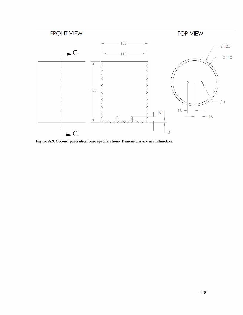
239

Figure A.9: Second generation base specifications. Dimensions are in millimetres.

240

Figure A.10: Second generation cap specifications. Dimensions are in millimetres.

Documents

SLAGGING IN ENTRAINED-FLOW GASIFIERS · th gasifier, five gasification tests were completed with the characterized coals. Solid samples from the refractory liners, in-situ gas sampling