sLH

C-P

roje

ct-N

ote-

0044

14/0

7/20

16

sLHC-Project-Note-0044

July 14, 2016

kai.papke@cern.ch

ANSYS modeling of thermal contraction of SPLHOM couplers during cool-down

K. PapkeBeams Department

Keywords: HOM Coupler, SPL, High-Gradient, Thermal Contraction, APDL

Summary

During the cool-down the HOM coupler as well as the cavity inside the cryo moduleexperience a thermal contraction. For most materials between room temperature andliquid helium temperatures, the changes in dimension are in the order of a few tenths ofa percent change in volume. This paper presents the effect of thermal contraction on theRF transmission behavior of HOM couplers, and in particular the influence on its notchfilter. Furthermore the simulation process with APDL is explained in detail. Conclusionsabout the necessary tuning range of the notch filter are made which is especially a concernfor couplers with only notch filter.

1 Introduction

The thermal contraction or expansion as one of the typical state functions to de-scribe a material thermodynamically, can be defined either by the volume expansivity βaccording to the following formula:

β =1

V

(

∂V

∂T

)

p

, (1)

or by the linear thermal expansion coefficient α which is a more appropriate form incase of solids as the changes in individual directions can be different. The linear thermalexpansion coefficient is defined as:

α =1

L

(

∂L

∂T

)

p

. (2)

This value is tabulated in the literature and for isotropic materials is linked to the volumeexpansivity via: β = 3α. Moreover, it is common in literature to relate the overallcontraction or expansion to 293K which can be derived from α according to:

L293 − LT

L293

=

ˆ T

293K

α(T )dT (3)

This is an internal CERN publication and does not necessarily reflect the views of the CERN management.

One of the major concerns is the effect of the differential thermal contraction and the asso-ciated thermal stress that may occur when two dissimilar materials are bonded together.In figure 1, the linear thermal expansion coefficient is shown for different materials. Thecontraction can vary in a large range between the materials as for example by a factor oftwo between niobium and copper leading to thermal stresses if they are bound together.The currently considered HOM couplers will be fabricated out of only one material, whichis either copper (prototype fabrication in progress) or later niobium. However, the nu-merical analysis presented in this paper can be applied to composite couplers, as well.In spite of the minor dimensional changes in a range of a few tenths of a millimeter per

0 50 100 150 200 250 300

Temperature [K]

0

50

100

150

200

250

300

350

L293−LT

L293

10−5

0 50 100 150 200 250 3000.00

0.25

0.50

0.75

1.00

1.25

1.50

1.75

α10−5[1/K]

αCu

αSteel

αNb

Figure 1: In dashed, the linear thermal expansion coefficient α for copper, niobium and stainlesssteel (AISI 304). The data are taken from [4]. In solid, the overall contraction with a referencetemperature of 293K.

meter, the effect on the notch filter may be notable and requires a tuning after cool-downor a detuning beforehand in order to compensate the effect of the contraction on the RFtransmission behavior of the coupler.

In the following, the work flow of the combined thermal-electromagnetic simulationis presented and verified with other simulation tools. The simulations are carried outwith the ANSYS Parametric Design Language (APDL) as it covers a wide range of multi-physical and engineering problems applied on exactly the same model and mesh, whichavoids any interpolation of field loads from one mesh to another (e.g. RF simulationperformed on the contracted model). This is especially important if the structural changesare very small as for example the thermal contraction or the deformation due to Lorentzforce detuning. Alternatives such as ACE3P, COMSOL or nowadays also CST are notconsidered in this paper. Merely the latter one is used for verifications of the harmonicsolver of APDL.

APDL is a scripting language to automate common tasks in ANSYS. This involves

2

the creation of parametrized models, the mesh configuration and meshing itself, materialsetup, definition of boundary conditions and applying loads, simulation setup and a mul-tiplicity of post processing functions. It allows structural mechanical, thermodynamic,electromagnetic, and fluid dynamical analysis and, furthermore, all these in combinationcoupled on the model using precisely the same or originally deformed mesh. APDL alsooffers a wide range of standard scripting features such as repeating a command, macros(functions), if-then-else branching, do-loops, and scalar, vector and matrix operations.Moreover, all information about the mesh elements and even nodes including the localsolutions are accessible and extractable which allows a large flexibility for the data postprocessing. The most important commands for this are *GET and *VGET which are ex-plained in detail in the user guide of APDL [2].

In order to structure the work flow of the coupled simulation, different macros havebeen programmed according to the following tasks:

1. Basic setup which involves building and meshing of the model, definition of materialproperties (createModel.mac).

2. S-Parameter simulation of the original model at 293K (HarmOriginal.mac).

3. Steady state thermal simulation which gives the deformed mesh(ThermalStruct.mac).

4. S-Parameter simulation of the contracted model at 2K or at a different temperature(HarmDeformed.mac).

2 Model preparation

In this section we discuss the different parts covered by the macro createModel.macwhich involves the geometry, the material definition as well as the meshing.

2.1 Geometry

First, the macro createModel.mac imports the HOM coupler model [3], comingfrom CST, HFSS or other CAD tools as Standard ACIS Text (*.sat) or Standard ACISBinary (*.sab) file. IGES files (*.iges) require further processing to convert them to solidmodels. The widely used STEP file format (*.stp) seems not to be supported by APDL(V15). However, other formats such as CATIA V5 files can be imported. The ACIS filescontain the pure solid information, whereas in other formats (e.g. IGES) the solids aredisassembled in their surfaces and have to be rejoined during the import, which sometimesleads to geometry errors and problems with the mesh such as too fine elements aroundthe contact region between two solids. Hence, the SAT or SAB format for the modelimport is a more reliable and advisable option to avoid problems concerning meshing andsimulation time.

One major restriction of APDL with respect to modeling is the limited supportof geometries if they have rounded edges (at least up to version 15)1. The import and

1The most CAD programs provide a feature to round edges with a defined radius. Depending on thesoftware it is called for example ’blending’ (ANSYS DM, CST) or ’Fillet’ (HFSS).

3

meshing of models with such features is possible, however, neither Boolean operationsnor merging of faces between solids is supported if two or more rounded edges are joinedwith each other. Note that merging faces between solids is mandatory for a precise RFsimulations that include structural deformations of the model and its mesh. Because ofthis the coupler model was simplified as shown in figure 2 which slightly changed thetransmission behavior. However, we are rather interested in the relative change of the S21

curve due the cool-down than in the absolute position of the notch filter. Furthermore,

(a) (b)

Figure 2: a) Original design including the rounded edges as the prototypes and final couplerfeature. b) Modified model without rounded edges considered for the simulation.2 The connec-tion to the tube wall (tube not shown here) is also simplified as it would have no effect on thethermal contraction of the whole model. The same is true for the RF behavior.

the fixation of the coupler parts on the tube wall is simplified as shown in figure 2 toavoid very small mesh elements and to reduce the likelihood of inverse elements whichmay result from the thermal contraction simulation and may lead to problems for furtherRF simulations. Finally, the model consists of three main parts:

• The HOM coupler parts (depending on the coupler type two to three separatedsolids),

• the vacuum, and

• the tube wall.

It is advisable to import all parts as bulk solid parts and to subtract stepwise theparts from each other within APDL (e.g. the vacuum solid from the tube solid). Thisensures that the faces between connected solids are merged, hence, shared between eachother. In the following, the APDL code is shown, which is used for the import and thepreparation:

~SATIN ,file ,SAT ,,SOLIDS ! model import from file.sat

VSBV ,5,4,, delete ,keep ! subtract vacuum from tube

VSBV ,1,6,, delete ,keep ! subtract tube from coupler

VSBV ,2,6,, delete ,delete ! subtract tube from coupler

NUMCMP ,volu ! compress volume IDs

VSBV ,3,1,, delete ,keep ! subtract coupler from vacuum

VSBV ,5,2,, delete ,keep ! subtract coupler from vacuum

VSBV ,3,4,, delete ,keep ! subtract coupler from vacuum

NUMMRG ,all ! merge coincident items

NUMCMP ,volu ! compress volume IDs

2We later found that rounded edges along the capacitor plate (here in horizontal direction) are possibleas long as they are not connected with any other rounded edges. This model extension reflects the RFbehavior of the original design much better and has been used in section 7.

4

To identify solids and to associate them with their ID, one can use the command /pnum,volu,1

and vplot which makes the IDs visible in the graphical user interface (GUI). The codeabove removes the tube wall because it is not necessary to consider the wall as solid inAPDL. Instead, one can apply shell elements meshed only on the surface of the vacuumpart to model the wall (see section 4). Using shell elements reduces the numerical effortnotably.

Moreover it is helpful to define components in APDL in order to select assembliesof volumes, areas, lines, elements or nodes. Here, we created the following components:

• coupler (volume assembly)

• vacuum (volume assembly)

• tube (area assembly)

The APDL code for the component creation with the corresponding volume and area IDsis as follows:

VSEL ,S,,,1,3 ! select coupler volume parts

CM,coupler ,VOLU ! create coupler component

VSEL ,S,,,4 ! select vacuum volume part

CM,vacuum ,VOLU ! create vacuum component

ASEL ,S,,,2 ! select 1st area of tube wall

ASEL ,A,,,31 ! add 2nd area to the selection

... ! add nth area to the selection

CM,tube ,AREA ! create tube component

2.2 Material Properties

We distinguish between two materials: i) The vacuum and ii) the material thecoupler and the tube is made of, which is either copper as considered for the first prototypeor niobium for later prototypes. The properties are summarized in table 1. We assume

Table 1: Material Properties at 293K

Parameter Unit APDL Vacuum Coupler

command (Cu) (Nb)

Permittivity MP,MURX 1 - -

Permeability MP,PERX 1 - -

Resistivity [nΩm] MP,RSVX - 15.9 -

Elastic modulus [GPa] MP,EX 0 117 104

Poisson’s ratio MP,PRXY 0.00 0.35 0.35

Lin. therm. expansion 10−5[1/K] MP,ALPX 0.00 1.68 0.70

Therm. conductivity [W/m/K] MP,KXX 0.0 394.0 54.5

a ‘slow’ cool-down, i.e. a quasi-stationary problem without any transient effects. Hence,we can neglect the heat transport and the temperature is everywhere the same duringcool-down.

5

The change of structural properties such as the elastic modulus and the Poisson’sratio in the considered temperature range is very low, so that the values are assumed tobe constant. The vacuum has to be considered for the thermal contraction simulation,as well. Hence, its material properties comprise also properties of the structural mechan-ics. Definitions for the permeability and permittivity are not necessary to model themetallic parts. The resistivity is mentioned only for completeness. We apply perfect elec-tric boundary conditions (PEC) for the RF simulations as surface loss will basically notchange the transmission behavior of the coupler. The temperature independent materialproperties can be defined in APDL as follows:

MP ,EX ,1 ,117 ! define elastic modulus of 117

! for the material with the ID 1

The linear thermal contraction, in contrast to all other considered properties, is temper-ature dependent (Fig.: 1), which is slightly more complicated to define in APDL. Anappropriate method is to load the temperature dependent values from an external fileinto an APDL table and to transfer the interpolated values at defined temperatures intothe material model. Tables in APDL are similar to arrays, however, the indices are realnumbers rather than integers. ANSYS calculates (through linear interpolation) any val-ues that fall between the explicitly declared array element values. The maximum numberof temperature points which can be defined for a material property is 100. Hence, theprocedure described above, using table array parameters as an intermediate step, is veryconvenient because the macro can define always 100 values equidistantly distributed from2K to 300K (e.g. for the linear thermal expansion α(T)) independent of the numberof values and the temperature range given in the input file. The following code readsthe tabulated data from a file which features eight columns in which the first one hasto represent the temperature points. The other columns are related to different materialproperties such as column number 7 corresponds to the linear thermal expansion.

toskip = 1 ! no. of lines to skip

/INQUIRE ,N,LINES ,file ,txt ! get no. of lines in file

toread = N - toskip ! no. of lines to read

*DEL ,tCu ,,NOPR ! delete pre - definition

*DIM ,tCu ,TABLE ,to_read -1,7 ! define table with

! 7 columns

*TREAD ,tCu ,file ,txt ,,toskip ! load file in table

*DO ,i ,1 ,100 ! iterate T-points

T = (i -1)*298/99+2 ! calculate temperature

DT = 293-T

MPTEMP ,i,T ! set temperature point

MPDATA ,ALPX ,2,, tCu(T ,7)/DT ! set property at T

*ENDDO

UIMP ,2, REFT ,,,293 ! reference temperature

In order to index the different properties within the APDL table (e.g. column number 7in the example above), the first line must contain indices (0, 1, 2, 3, ...). Hence, the inputfile has basically the following structure:

Listing 1: Structure of the material property file.

TEMP PROP1 PROP2 PROP3 PROP4 PROP5 PROP6 PROP7

0 1 2 3 4 5 6 7

2 8960 0.028 0.00 0.746 187 0 3.25E-3

10 8960 0.870 2.35 0.118 922 4470 3.25E-3

20 8960 7.270 35.4 0.024 1590 17400 3.25E-3

...

100 8960 251.0 10500 0.000 2449 87800 2.82E-3

...

6

280 8960 382 71800 0.000 395 1.6 E3 2.15E-4

290 8960 384 75600 0.000 395 1.7 E3 5.01E-5

293 8960 385 76800 0.000 394 1.7 E3 0.00

One important aspect for the thermal contraction simulation is that APDL interpretsthe material property ALPX not as the linear thermal expansion α(T) as defined in (2)but rather as the overall contraction related to a reference temperature divided by thedifference between the considered temperature and the reference temperature. Hence, itis defined as:

ALPX(T) =1

Tref − T

ˆ T

Tref

α(T )dT. (4)

As a consequence the material file must contain the integrated values and not the linearthermal expansion α(T) itself. In the example described above, the input file contains theaccumulated thermal contraction related to 293K according to equation (3) (solid linesin Fig. 1) as it is typically found in literature. The division by the temperature differenceis carried out within the macro when applying the value from the APDL table to thematerial property ALPX:

MPDATA ,ALPX ,2,, tCu(T ,7)/DT.

In figure 3, the temperature dependent contraction parameter ALPX is shown for differentmaterials.

0 50 100 150 200 250 300

Temperature [K]

0.4

0.6

0.8

1.0

1.2

1.4

1.6

1.8

ALPX

Tref = 293K

Copper

Steel AISI 304

Niobium

Figure 3: Temperature dependent contraction parameter ALPX for copper, stainless steel, andniobium which is used as the main parameter for the thermal contraction simulation in APDL.

2.3 Meshing

As a first step before meshing the model, the type of elements has to be defined.APDL offers a multiplicity of elements which differ for example in dimension (1D, 2Dand 3D), in shape (e.g. tetrahedral, hexahedral), in the order of ansatz functions (e.g.1st or 2nd order), and in degrees of freedom which specify elements to physical problems(e.g. thermodynamics, structural mechanics, RF). The ANSYS elements reference [1]

7

gives a detailed description of all available elements with respect to their application.The following code uses high frequency elements (Type: HF119) to mesh first the couplerparts and then the surrounding vacuum:

et ,1, HF119 ,2 ! define high frequency solid

! tetrahedral element , 2nd order

MAT ,2 ! select material: copper

CMSEL ,S,coupler ! select parts for meshing

LESIZE ,40,,,20 ! 20 elements along notch plate

LESIZE ,43,,,20 ! 20 elements along notch plate

ESIZE ,0.002 ! set max. element size

VMESH ,ALL ! mesh the selected volumes

MAT ,1 ! select material: vacuum

CMSEL ,S,vacuum ! select parts for meshing

ESIZE ,0.007 ! set max. element size

VMESH ,ALL ! mesh the selected volumes

The resulting mesh based on the code above is shown in figure 4. It features around250000 tetrahedral elements which is a good trade-off between simulation time and accu-racy. Several tests for convergence have been performed in order to estimate an appropri-ate number of elements. Under these conditions, the harmonic analysis (RF simulation)requires around three minutes per frequency point and the thermal contraction simula-tion needs around ten minutes in total. The bottleneck is finally the RF simulation as weconsider typically a few hundred frequency points in order to have a sufficient resolutionof the S-Parameter curve. The meshing itself requires only half a minute with the config-uration above. Mesh refinements using commands such as erefine,all,,,1 are possiblebut did not lead to better meshes in our case.

Note: The faces between connected solids are merged as described before. Hence,also the elements share the corresponding faces and nodes.

The macro createModel.mac creates the root project which is the base for all of the

X Y

Z

File: HBB_DN2C_HSV1_simplified33

(a)

X Y

Z

File: HBB_DN2C_HSV1_simplified33

(b)

Figure 4: a) The HOM coupler parts which are meshed with approximately 100000 elements.b) The vacuum part which is meshed with around 150000 elements.

8

following simulations. This root project provides each problem type (e.g. thermal, struc-tural mechanics, and RF simulations) with the model, the mesh, and material properties.In the following all described macros will load the root project but create sub projects toseparately save all modifications, adaptions, and preparations for the individual simula-tions, as well as the results.

3 RF Simulation

To simulate S-Parameters, APDL offers a wide spectrum of features3. This involvesperfect electric (PEC) and magnetic boundary (PMC) conditions, impedance boundaryconditions, definition of lumped circuit elements, perfect matched layer (PML), and waveguide ports.

3.1 Boundary conditions and wave guide ports

We neglect any losses on the coupler surface not only if niobium is considered inits superconducting state but also in case of copper as the electrical conductivity of5.96× 107 S/m is too high to notably impact the field configuration and, hence, the S-Parameters. Therefore all boundaries of the HOM coupler are configured as PEC and thecoupler parts can be excluded from the simulation such that only the vacuum is takeninto account. Furthermore, a circular waveguide port is defined on the antenna side ofthe model which excites TM or TE modes, respectively. On the opposite side which isthe output of the HOM coupler we define a coaxial waveguide to transmit TEM-modesout of the structure. Figure 5 depicts the configuration for the RF simulation.

V1

V2

V3

V411

X

Y

Z

Figure 5: Setup for the S-Parameter simulation. Terminating the end of the HOM coupler tubetowards the beam pipe with a circular waveguide port (red) allows the excitation of monopoleas well as dipole modes, whereas a TEM mode is transmitted out of the coaxial output (blue).PEC boundary conditions are applied to all other surfaces.

The following code is used to setup all boundary and excitation conditions.

3One has to use mesh elements of the type HF119 or HF118 [1] as they provide the correspondingdegrees of freedom for electromagnetic problems.

9

CMSEL ,S,vacuum ! select all surfaces

DA ,ALL ,AX ,0 ! configure as PEC

! define coaxial wave guide port with TEM -mode

ASEL ,S,,,30 ! select 1st port face

SFA ,ALL ,,PORT ,1 ! declare as port no. 1

HFPORT ,1,COAX ,11,TEM ,EXT ,ri,ra ,1,0 ! configuration

! define circular wave guide port with TM01 -mode

ASEL ,S,,,41 ! select 1st port face

SFA ,ALL ,,PORT ,2 ! declare as port no. 2

HFPORT ,2,CIRC ,11,TM01 ,EXT ,rad ! configuration

Note: It is mandatory to configure the circular wave guide with pseudo dimensions insuch a way that the cut-off frequency of the waveguide is below the simulation frequency.The cut-off frequency is computed analytical by APDL based on the configured radius inthe HFPORT command. It does not refer to the real radius of the model. In general, theharmonic solver fails and produces an error message if the considered frequency point isbelow the cut-off frequency of a wave guide port. As the considered TM01 mode at thecircular wave guide has a cut-off frequency of 5.1GHz we have to define virtually a muchlarger radius to analyze the transmission behavior between 0.5 and 2.5GHz.

3.2 Harmonic analysis and verification

A disadvantage of APDL is the performance of the harmonic solver to computeS-Parameters over a frequency range. The solver needs approximately three minutes tocompute the scattering parameter for one frequency point whereas CST requires a fewminutes for 10001 frequency points, and HFSS around 10-15 minutes for a comparablenumber of mesh elements. In order to reduce the simulation time and to efficientlyuse the computational resources of a work station, it is advisable to split the frequencysweep in separated simulations which can be executed in parallel (Fig. 6). This also

0.5 1.0 1.5 2.0 2.5

Frequency[GHz]

−180

−160

−140

−120

−100

−80

−60

−40

−20

0

S21[dB]

Figure 6: RF transmission behavior of the exemplary HOM coupler. The frequency sweep wassplit into 13 ranges in order to reduce simulation time.

allows to vary the frequency resolution over the considered frequency range. In table2, the resolution with respect to the frequency range is listed as well as the number ofsimulations (accumulated number of sweeps) which can be carried out in parallel. Theresults of APDL agree well with CST and HFSS (Fig. 7). A slight offset of around 1.5 dBappears for the S-Parameters calculated by APDL. However, the frequency of the notchesdiffers by less than 0.2%, which is the commonly used convergence criterion for scattering

10

parameter calculations in RF applications. Due to the modifications in the geometry(2.1), the notch filter is located at 680.0MHz instead of 704.4MHz (Fig. 7 b). This is nota problem as we are interested in the relative change, which means the detuning of thenotch filter during cool-down.

4 Thermal contraction of couplers without stainless steel flanges

In this first step we study the deformation of the coupler itself without consideringits stainless steel flanges. These will be taken into account in a 2nd step of the analysisin section 6. Independent of the previously described harmonic analysis, the thermal

Table 2: Frequency resolution for the S-Parameter calculations.

Frequency range ∆f No. of sweeps No. of points per sweep

500...600MHz 1.0MHz 1 101

600...700MHz 0.1MHz 5 201

700...1000MHz 1.0MHz 3 103

1000...1400MHz 2.0MHz 2 101

1400...2600MHz 6.0MHz 2 101

0.5 1.0 1.5 2.0 2.5

Frequency [GHz]

−180

−160

−140

−120

−100

−80

−60

−40

−20

0

S21[dB]

APDL

CST

HFSS

(a)

0.60 0.62 0.64 0.66 0.68 0.70 0.72 0.74

Frequency [GHz]

−180

−160

−140

−120

−100

−80

−60

S21[dB]

APDL

CST

HFSS

(b)

0.86 0.88 0.90 0.92 0.94

Frequency [GHz]

−50

−45

−40

−35

−30

−25

−20

−15

−10

S21[dB]

APDL

CST

HFSS

(c)

1.10 1.15 1.20 1.25 1.30 1.35 1.40

Frequency [GHz]

−25

−20

−15

−10

−5

0

S21[dB]

APDL

CST

HFSS

(d)

Figure 7: Comparison of the S-Parameter calculations between APDL, CST, and HFSS. a)The whole frequency range from 0.5 to 2.5GHz. b) S21 around the fundamental pass band(notch filter). c) S21 at the 1st dipole band (∼920MHz). d) S21 around the 2nd monopole band(∼1.33GHz).

11

contraction simulation is carried out. Hence, it can run in parallel to the RF simulation.For this purpose the macro ThermalStruct.mac is used.

4.1 Mesh extension and boundary conditions

First the macro modifies the element type (after loading the root project) to changethe problem type from RF to structural thermal analysis. In this case one may change theHF119 elements to SOLID187 elements [1]. In addition, we use the shell elements SHELL281in order to efficiently model the coupler tube. A modeling with three dimensional elementsis computationally much more expensive. These two-dimensional elements can be directlymatched to the mesh of the vacuum tube on the surface. The following code applies theelement modification and configuration, as well as meshing of the coupler tube.

ET ,1, SOLID187 ,2 ! HF119 -> SOLID187 elem.

ET ,2, SHELL281 ! add shell element (ID 2)

TYPE ,2 ! select element type

MAT ,2 ! set active material (Cu)

SECTYPE ,1, SHELL ! Shell element setup

SECDATA , 0.0024 ,2 ,0.0 ,5 ! shell thickness 2.4mm

! and 5 integration points

SECOFFSET ,BOT ! offset to bottom

CMSEL ,S,tube ! select tube areas

MSHAPE ,1,2D ! setup 2D triangle mesh

AMESH ,all ! mesh shell elements

ANORM ,40,0 ! correct face orientation

The shell elements have to be configured with material information and parameters suchas thickness, offset position and number of integration points (the numerical integrationmethod is Simpson’s Rule). Sometimes it is necessary to flip or correct the orientation ofshell elements if they vary with respect to each other. This is not important for thermalcontraction simulations but rather in case of vectorial loads such as forces, pressure, andmomentum. The command ANORM aligns all selected elements to the normal vector of aspecified area.

In figure 8, the mesh is shown, which is used for the thermal contraction analysis.The vacuum elements are hidden for a better visualization. They have to be included inthe simulations. Otherwise the deformed mesh will be corrupted if only the elements atthe coupler and tube surface deform. ANSYS announced for the newest version (v16) afeature which avoids the creation of inverse elements. Hence, it might be possible in thefuture version to exclude vacuum elements from the contraction simulation, which wouldreduce the calculation time notably from 10 minutes to less than one minute.

Furthermore, the boundary conditions for the thermal solver have to be defined,which consist of two parts. i) Select the elements and nodes to which the bound-ary conditions shall be applied. Then define the final temperature using the commandBF,ALL,TEMP,3. ii) The mechanical fixation of the model to restrict the degrees of free-dom. The coupler is fixed at the coaxial output as the contraction in that region doesnot change the frequency response. Such a fixation will be applied on the selected nodesusing the command D,ALL,ALL.

12

X

Y

Z

Figure 8: Mesh for the thermal contraction simulation including shell elements to model thecoupler tube (Thickness: 2.4mm).

4.2 Structural thermal Analysis

In order to verify the results of the simulation, the displacement of key points (spe-cific nodes of the model which are depicted in figure 9) was calculated at different tem-peratures from 293 down to 2K always in comparison to the initial temperature of 293K.The following code fragment is an example of how to access the number of key points,the corresponding node IDs, and finally the coordinates of each node.

*GET , nKP , KP , 0, count ! get number of key points

nKP = nKP + 1 ! 1 additional point

*DIM ,KPPOSX ,,nKP ! vector for key points X

*DIM ,KPPOSY ,,nKP ! vector for key points Y

*DIM ,KPPOSZ ,,nKP ! vector for key points Z

*DIM ,KPtoN ,,nKP ! vector key point -> node

*VGET ,KPtoN (1),KP ,,ATTR ,NODE ! get node of key points

pnt = x1 ,y1 ,z1 ! point on the notch plate

*MOPER ,KPtoN(nKP ),pnt ,NNEAR ! get ID of nearest node

! and add to list

*DO ,i,1, nKP ! get x,y,z coordinates

*GET ,KPPOSX (i,1), NODE ,KPtoN(i),LOC ,X

*GET ,KPPOSY (i,1), NODE ,KPtoN(i),LOC ,Y

*GET ,KPPOSZ (i,1), NODE ,KPtoN(i),LOC ,Z

*ENDDO

A build-in matrix operation (*MOPER) is used to seek the nearest node to user definedcoordinates. This feature is used to analyze the contraction of the notch filter gap whereno key point exist (Fig. 9).

In figure 10, the results of the thermal contraction are shown for different partsof the coupler assuming copper as material. It shows the overall contraction with areference temperature of 293K to be consistent to formula (3), or typical literature values,respectively. The results are in a good agreement with the curve shown in figure 1. Thereare minor deviations with respect to the contractions of the gaps of the notch filter andof the feed-through capacitor (C1) whose dimensions are less than 0.7mm.

13

37

3839

710

353436

34 3536

38

37

3938

3536

39

35

3839

36

3332

7

3233

1010

3332

7

4340

4142

41

4043

42

40

4142

43

29

28

31

30

5352

28

3127

24

3026

2731

2529

3026

2824

2529

24

25

26

27

2223

53

89

52

22

1311

23

1817

1916

1718

8

5352

9

13

2223

11

8

1113

9

191615

1414

89

1516

1718

19

620

21

1

206

5

21

11

1243

13

8

1415

9

13

3 212

11

2

1

21

5

4 12

1

234

5

620

6

5

21

620

21

11

234

5

6

2

1

21

5

4 12

8

1415

9

13

3 212

11

8

1113

9

53

89

52

44

45

46

47

710

5352

8

5352

9

14

89

1516

1718

19191615

141916

171818

17

7

3233

1010

3332

7

35

3839

36

3332

34 3536

353436

38

3536

39

37

3839

38

37

39

44

47

49

50

48

49

50

51

48

514340

41

4043

4241

42

40

4142

43

49

48

51

50

45

44

47

46

45

46

22

1311

23

24

25

26

27

2223

13

2223

1111

1243

13

28

3127

24

3026

2731

2529

3026

29

28

31

30

2824

2529

XY

Z

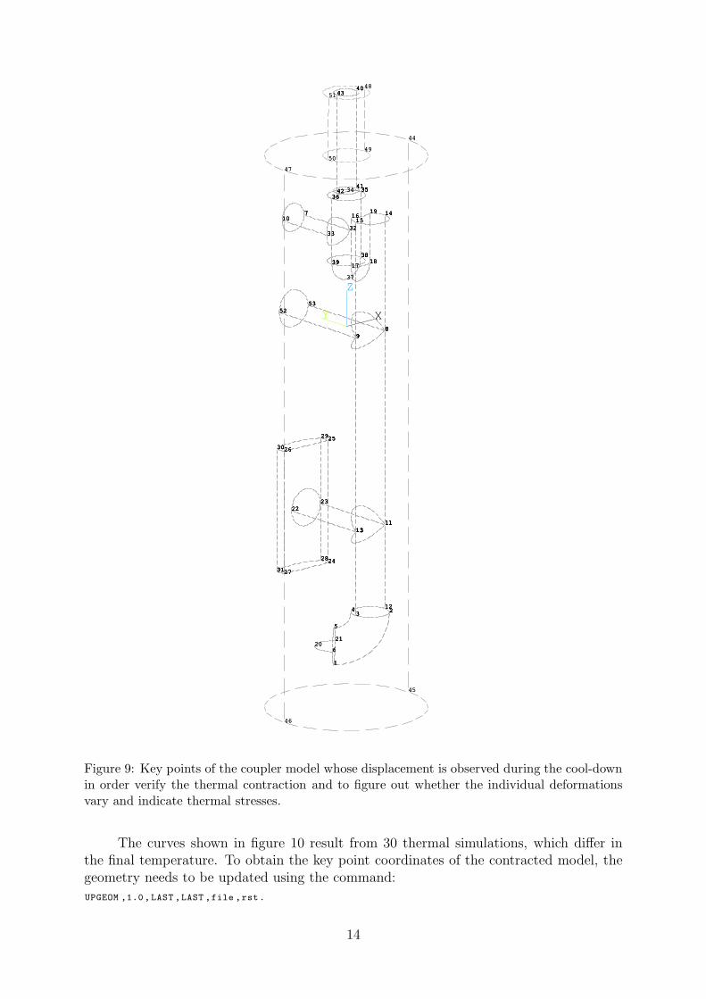
Figure 9: Key points of the coupler model whose displacement is observed during the cool-downin order verify the thermal contraction and to figure out whether the individual deformationsvary and indicate thermal stresses.

The curves shown in figure 10 result from 30 thermal simulations, which differ inthe final temperature. To obtain the key point coordinates of the contracted model, thegeometry needs to be updated using the command:

UPGEOM ,1.0, LAST ,LAST ,file ,rst.

14

0 50 100 150 200 250 300

Temperature [K]

0

50

100

150

200

250

300

350

L293−LT

L293

10−5

Tube diameterAntenna lengthAntenna diameterNotch heightNotch widthNotch gapC1 gapC2 gap

Figure 10: Accumulated thermal contraction of individual parts of the HOM coupler with respectto 293K. C1 is the uppermost capacitor at the feed-through. C2 is the horizontal capacitor.The antenna length is measured between key point 3 and 15 and its diameter between key point8 and 9.

This command loads the result file ’file.rst’ from the previous executed simulation, whichcontains all node displacements and applies them onto the original mesh.

In table 3, the absolute contractions in x, y and z direction are shown accordingto the Cartesian coordinate system in figure 9. The values are represented generally asdisplacements to distinguish between the positive and negative axes because not all partsof the coupler are in the center of the tube. Hence, for example the maximum contractionin the negative y direction differs from the one in the positive y-direction. All valuesare related to a cool-down from 293K to 2K and to a coupler made of copper. Thedisplacements are also graphically shown in figure 11 together with the original mesh.

Table 3: Deformation of the HOM coupler.

Dimension Unit Positive axis* Negative axis*

∆x [µm] -26.0 40.4∆y [µm] -73.3 49.8∆z [µm] 0.0 528.0

* The coordinate system is in the tube center (Fig. 9).

15

-26 -11 4 19 34

∆x [µm]

MN

MX

X

Y

Z

(a)

-70 -40 -10 20 50

∆y [µm]

MN

MX

X

Y

Z

(b)

0 125 250 375 500

∆z [µm]

MN

MX

X

Y

Z

(c)

Figure 11: Contraction of the HOM coupler in x, y and z-direction (sub-figures a, b, c) . Thedisplacements are scaled by a factor of 10 to illustrate the contraction with respect to the originalmesh.

16

4.3 S-Parameter shift

Finally, a harmonic analysis is carried out on the contracted geometry. The onlydifference to the analysis of the original model is the conversion of the structural thermalelements SOLID187 back to the high frequency elements HF119 in the same manner asdescribed before. In addition, the shell elements have to be excluded from the RF sim-ulation as they are not supported by the harmonic solver. The impact of the thermalcontraction is shown in figure 12. The notch filter shows a detuning of around 2MHz,

0.5 1.0 1.5 2.0 2.5

Frequency [GHz]

−180

−160

−140

−120

−100

−80

−60

−40

−20

0

S21[dB]

T = 293K

T = 2K

(a)

0.600 0.625 0.650 0.675 0.700 0.725 0.750

Frequency [GHz]

−180

−160

−140

−120

−100

−80

−60

S21[dB] ∆f0 = 2.1MHz

∆f1 = 2.1MHz

∆f2 = 2.0MHz

T = 293K

T = 2K

(b)

0.850 0.875 0.900 0.925 0.950

Frequency [GHz]

−50

−45

−40

−35

−30

−25

−20

−15

−10

S21[dB]

∆f3 = 3.0MHz

T = 293K

T = 2K

(c)

Figure 12: Simulated variation of S21 due to the thermal contraction. a) S21 between 0.5 and2.5GHz b) Detuning of the notch filter by around 2MHz. c) S21 shift at the 1st dipole band(920MHz).

17

which is a lot especially in case of a single notch filter. The considered double notch filter,however, is robust enough to guarantee more than 100 dB damping after detuning. Theresonance at the first dipole band is shifted by 3 MHz and this shift should certainly betaken into account, when tuning the coupler at warm. In general, the coupler frequenciesare shifted to towards higher values and the shift increases with the frequency.

5 Comparison between the HOM Couplers

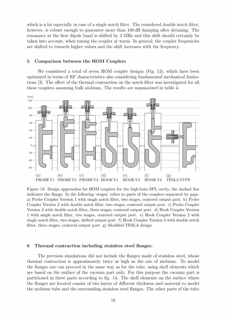
We considered a total of seven HOM coupler designs (Fig. 13), which have beenoptimized in terms of RF characteristics also considering fundamental mechanical limita-tions [3]. The effect of the thermal contraction on the notch filter was investigated for allthese couplers assuming bulk niobium. The results are summarized in table 4.

-60

-40

-20

0

20

40

60

80

100

120

[mm]

(a)PROBEV1

(b)PROBEV2

(c)PROBEV3

(d)HOOKV1

(e)HOOKV2

(f)HOOKV3

(g)TESLATYPE

Figure 13: Design approaches for HOM couplers for the high-beta SPL cavity, the dashed lineindicates the flange. In the following ‘stages’ refers to parts of the couplers separated by gaps.a) Probe Coupler Version 1 with single notch filter, two stages, centered output port. b) ProbeCoupler Version 2 with double notch filter, two stages, centered output port. c) Probe CouplerVersion 3 with double notch filter, three stages, centered output port. d) Hook Coupler Version1 with single notch filter, two stages, centered output port. e) Hook Coupler Version 2 withsingle notch filter, two stages, shifted output port. f) Hook Coupler Version 3 with double notchfilter, three stages, centered output port. g) Modified TESLA design.

6 Thermal contraction including stainless steel flanges.

The previous simulations did not include the flanges made of stainless steel, whosethermal contraction is approximately twice as high as the one of niobium. To modelthe flanges one can proceed in the same way as for the tube, using shell elements whichare based on the surface of the vacuum part only. For this purpose the vacuum part ispartitioned in three parts according to fig. 14. The shell elements on the surface wherethe flanges are located consist of two layers of different thickness and material to modelthe niobium tube and the surrounding stainless steel flanges. The other parts of the tube

18

Table 4: Notch detuning for the concidered HOM couplers.

Coupler Primary notch Secondary notchdesign f293K [MHz] f2K [MHz] ∆f [MHz] f293K [MHz] f2K [MHz] ∆f [MHz]

PROBE V1 675.00 675.95 0.950 - - -PROBE V2 644.05 644.85 0.800 691.20 692.15 0.950PROBE V3 639.60 640.60 1.000 681.35 682.30 0.950HOOK V1 778.95 780.15 1.200 - - -HOOK V2 778.05 779.15 1.100 - - -HOOK V3 636.30 637.20 0.900 724.75 725.80 1.050TESLA 640.40 641.30 0.900 - - -

surface are handled as before using shell elements which consist only of one layer to modelthe niobium tube.

1

X

Y

Z

Displacement superposition of x, y and z (DSCALE = 20)

ELEMENTS

Figure 14: Partition of the coupler model with corresponding shell elements. In the middlesection the shell consist of two layers of different material. One layer of 2.4mm thickness tomodel the niobium tube and a second layer of 10mm thickness to model the stainless steelflanges. The other two sections contain only the first layer.

-70 -35 0 35 70

∆y [µm]

X

Y

Z

Figure 15: Contraction of the HOM coupler, tube and flanges in y-direction. The displacementsare scaled by a factor of 10 to illustrate the contraction with respect to the original mesh.

19

The bigger contraction of the flanges changes the detuning of the notch filter from+1.0MHz to −2.7MHz for the PROBE V3 coupler. The detuning of the HOOK V3 cou-pler changes from +1.05MHz to −8.7MHz. Instead of increasing as before, the frequencyof the notch resonances is now decreasing during cool-down. This is caused by the chang-ing gap distance between the capacitor plate and the tube wall. The same tendency canbe assumed for the other models in section 5 except for the TESLA design. Therefore, theflanges play an important role for the thermal contraction and have to be included in thesimulation. We further looked at the contraction of the notch filter with respect to thetube wall to explain the different behavior between the PROBE V3 and the HOOK V3coupler whose notch plates are identical (Fig. 17). The only difference is the connection

0.62 0.63 0.64 0.65 0.66 0.67 0.68 0.69 0.70

Frequency [GHz]

−170

−160

−150

−140

−130

−120

−110

−100

−90

S21[dB]

∆f0 = −0.500MHz

∆f1 = −2.700MHz

T = 293K

T = 2K

0.62 0.64 0.66 0.68 0.70 0.72 0.74

Frequency [GHz]

−160

−150

−140

−130

−120

−110

−100

−90

−80

S21[dB]

∆f0 = −1.600MHz

∆f1 = −8.700MHz

T = 293K

T = 2K

Figure 16: Simulated Notch detuning taking into account the different contraction of the stainlesssteel flanges. Upper: PROBE V3. Lower: HOOK V3.

via the hook in the latter case. Figures 18 and 19 show the distance between the notchplate and the tube wall before and after thermal contraction. Apparently the fixation ofthe plate via hook results in more change of the notch gap during cool-down. In averagethe gap distance reduces by 0.041mm for the HOOK V3 coupler whereas 0.016mm forthe PROBE V3 coupler. Correspondingly the frequency shift for the HOOK V3 coupleris three times higher as the change of gap distances is linear correlated to the frequencyshift for small values (∆L ≪ L).

20

As a comparison we did a sensitivity analysis of the notch resonances as a functionof the gap distance. The S-Parameter simulations for variing gap distance yield similarfrequency shifts. However the results differ by up to 50% as this type of simulation onlyconsider a change of the gap distance and not the overall contraction.

z

x

Tube wall

Notch filter plate

y

Figure 17: Schematic of the notch filter close to the tube wall.

−8−4

04

8 010

2030

0.7

0.8

0.9

1.0

x [mm]

z [mm]

y [mm]293 K2 K

(a)

0 5 10 15 20 25 30 35

z [mm] (vertical axis)

0.665

0.670

0.675

0.680

0.685

0.690

0.695

0.700

0.705

ym

in[m

m](notchgap) ∆L = 0.016 mm

293 K

2 K

(b)

Figure 18: Analysis of the notch filter for the PROBE V3 coupler. a) 3D profile of the distancebetween notch plate and tube wall at 293K and 2K. b) A slice of the 3D profile in (a) at x = 0(minimum distance between notch plate and tube wall. On average the gap distance reduces by0.016mm.

−8−4

04

8 0

10

20

30

0.8

0.9

1.0

1.1

x [mm]

z [mm]

y [mm]293 K2 K

(a)

0 5 10 15 20 25 30

z [mm] (vertical axis)

0.79

0.80

0.81

0.82

0.83

0.84

0.85

0.86

ym

in[m

m](gap)

∆L = 0.041 mm

293 K

2 K

(b)

Figure 19: Analysis of the notch filter for the HOOK V3 coupler. a) 3D profile of the distancebetween notch plate and tube wall at 293K and 2K. b) A slice of the 3D profile in (a) at x = 0(minimum distance between notch plate and tube wall. On average the gap distance reduces by0.041mm.

21

7 Measurement of the Notch Detuning during Cool-Down

Finally, we measured the frequency shift of a prototype (PROBE V3) cooled downto 77K with liquid nitrogen. The prototype is made of copper and equipped with arotatable stainless steel flange (welded). A coaxial transmission line on which a SPLHOM coupler can be mounted serves as test facility to measure the filter characteristicsinside and outside the nitrogen bath. This test facility has the shape of a cross, featuringfour ports: The input and output port of the transmission line, in which the latter oneis matched with a 50Ω load. The remaining two ports perpendicular to the transmissionline are used for the HOM coupler and a vacuum valve. The assembly is shown in figure20. We have not used liquid helium to further cool down the coupler as the purpose ofthis test is the verification of the simulation and the quantitative estimate of its accuracy.Furthermore this copper prototype will not be used for any cavity cold test. Neverthelessat 77K more than 90% of the maximum contraction is done such that our measurementallows a good estimate of the frequency shift at 2K.

(a) (b)

Figure 20: a) Measurement setup. The HOM coupler is located on the bottom side of the cross.The network analyzer measures the transmission from the input of the coaxial transmission line(left) to the output of the HOM coupler. The second port of the coaxial line (right) is terminatedby a 50Ω load. b) The whole assembly plunged into the nitrogen bath cooling the coupler downto 77K.

The network analyzer was configured with an intermediate frequency bandwidth(IFBW) of 10Hz and 10001 frequency points over a span of 80MHz around 705MHzcenter frequency. Due to the high attenuation, a large number of points and the lowintermediate frequency bandwidth are necessary in order to measure the notch resonancesprecisely. The results of the measurements are shown in figure 21 and compared with asimulation in APDL taken into account the stainless steel flange welded on the coppertube. Indeed, they show an excellent agreement within an accuracy of 10%. Also thedifferent shifts of the two resonances is well represented by the simulation. Note that theabsolute values differ as it is not possible to create an exact model of the HOM couplerin APDL (see section 2.1).

22

0.66 0.67 0.68 0.69 0.70 0.71 0.72 0.73 0.74

Frequency [GHz]

−160

−150

−140

−130

−120

−110

−100

−90S21[dB]

∆f0 = 2.300MHz

∆f1 = 2.900MHz

T = 293 K

T = 77 K

(a) (b)

Figure 21: Notch detuning of the copper prototype HOM coupler (PROBE V3) simulates (a)and measured (b).

8 Conclusions

The thermal contraction of SPL HOM couplers during cool-down was investigatedby simulations using ANSYS APDL. All necessary aspects of the simulation which is basedon a parametric design language were described in details in order to modify and to applythe existing scripts to other projects. The main focus of this paper was the evaluation ofthe detuning of the notch filter of different HOM couplers considered for the SPL high-beta superconducting cavities. First, the flange was excluded from the model which ledto a detuning of 0.8 to 1.2MHz. Hence, the influence of the thermal contraction on thenotch filter only slightly depends on the geometry but rather on the material. Couplerswith double notch filter easily handle this detuning whereas the single notch filters wouldrequire a corresponding tuning before the cool-down in order to compensate the effect ofthe thermal contraction. The filter characteristics of the couplers, which are tuned to allowhigh transmission for certain HOM frequency bands should also be pre-tuned taking intoaccount the changes due to the cool-down. Finally the model was extended consideringalso the stainless steel flanges as they are located at the same position as the notch filter.Due to the higher contraction of the flanges the detuning of the notch filter changes from+1MHz to −2.7MHz for the PROBER V1 coupler which is still not a problem for itsdouble notch filter due to the high bandwidth. Moreover the frequency of the notchfilter is reduced instead of increased when considering the flanges. The designs with ahook are more affected by the contraction of the flanges. For the HOOK V3 coupler, thedetuning of the notch filter changes from +1.05MHz to −8.7MHz. Finally, we verifiedour simulations for a PROBE V3 coupler prototype made of copper whose measurementsshow an agreement within 10%. At least in this case, the APDL simulations seem to bevery reliable but they still need verification in the case for niobium couplers where thechange of the notch resonances behaves very differently according to the simulations.

References

[1] ANSYS Inc. ANSYS Mechanical APDL Element Reference, 2013.

[2] PADT Inc., Jeff Strain, and Eric Miller. Introduction to the ANSYS Parametric DesignLanguage (APDL): A Guide to the ANSYS Parametric Design Language. CreateSpaceIndependent Publishing Platform, USA, 1st edition, 2013.

23

[3] K. Papke, F. Gerigk, and U. van Rienen. HOM Couplers for CERN SPL Cavities. InProc. SRF2013, pages 1066–1068, 2013.

[4] R.P. Reed, A.F. Clark, and American Society for Metals. Materials at low tempera-tures. American Society for Metals, 1983.

24