Slide 1

Business and Economic ForecastingChapter 5

Business and Economic Forecasting is a critical managerial activity which comes in two forms:

Quantitative Forecasting +2.1047%Quantitative Forecasting +2.1047% Gives the precise amount

or percentage

Qualitative ForecastingQualitative Forecasting Gives the expected direction Up, down, or about the same

2008 Thomson * South-Western

Slide 2

Managerial ChallengeExcess Fiber Optic

Capacity• High-speed data installation

grew exponentially• But adoption follows a typical

S-curve pattern, similar to the adoption rate of TV

• Access grew too fast, leading to excess capacity around the time of the tech bubble in 2001

• The challenge is to predict demand properly

1940 1960 1980 2000 2020

100% Color TVs

InternetAccess

Slide 3

The Significance of Forecasting• Both public and private enterprises operate under

conditions of uncertainty. • Management wishes to limit this uncertainty by predicting

changes in cost, price, sales, and interest rates. • Accurate forecasting can help develop strategies to

promote profitable trends and to avoid unprofitable ones. • A forecast is a prediction concerning the future. Good

forecasting will reduce, but not eliminate, the uncertainty that all managers feel.

Slide 4

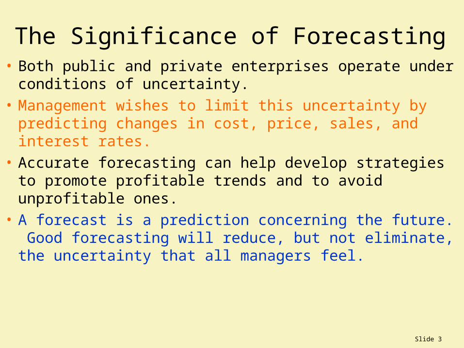
Hierarchy of Forecasts• The selection of forecasting techniques depends in part on

the level of economic aggregation involved.

• The hierarchy of forecasting is:

• National Economy (GDP, interest rates, inflation, etc.)

»sectors of the economy (durable goods) industry forecasts (all automobile manufacturers)

> firm forecasts (Ford Motor Company)

»Product forecasts (The Ford Focus)

Slide 5

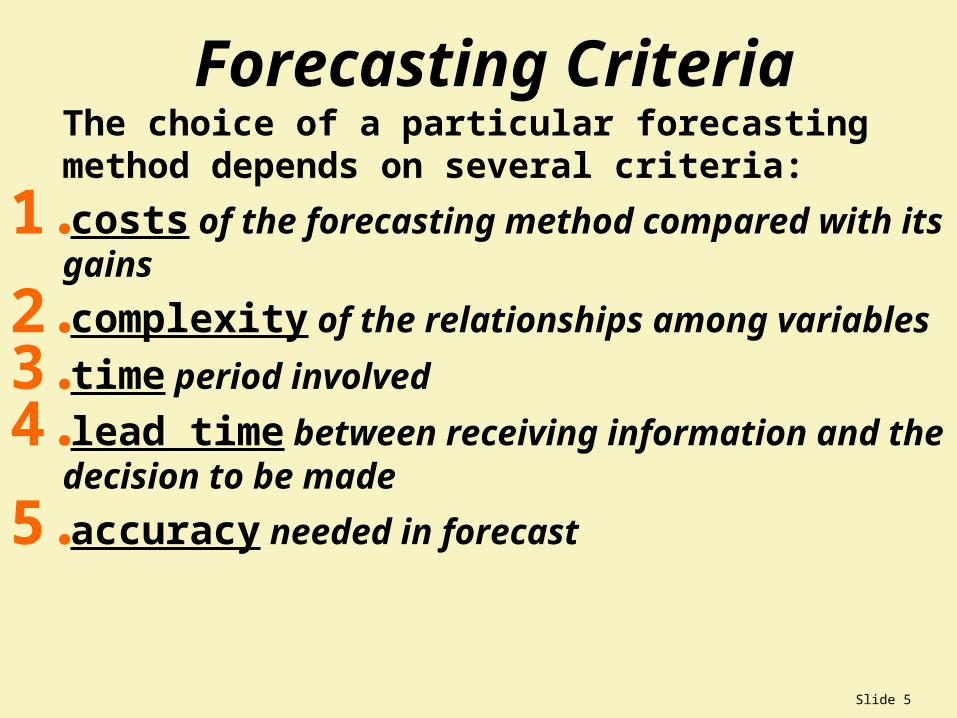
Forecasting CriteriaThe choice of a particular forecasting method depends on several criteria:

1.costs of the forecasting method compared with its gains

2.complexity of the relationships among variables

3.time period involved

4.lead time between receiving information and the decision to be made

5.accuracy needed in forecast

Slide 6

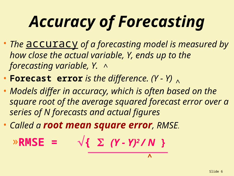
Accuracy of Forecasting• The accuracy of a forecasting model is measured by how

close the actual variable, Y, ends up to the forecasting variable, Y.

• Forecast error is the difference. (Y - Y)

• Models differ in accuracy, which is often based on the square root of the average squared forecast error over a series of N forecasts and actual figures

• Called a root mean square error, RMSE.

»RMSE = { (Y - Y)2 / N }

^

^

^

Slide 7

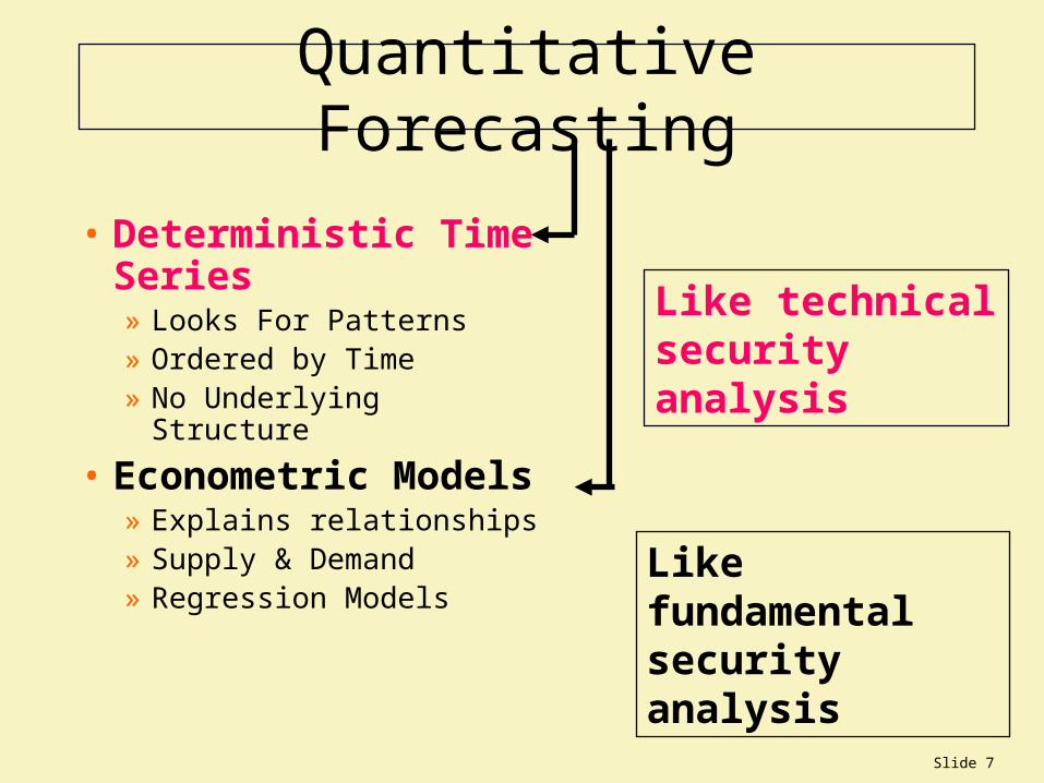
Quantitative Forecasting

• Deterministic Time Series » Looks For Patterns» Ordered by Time» No Underlying Structure

• Econometric Models» Explains relationships» Supply & Demand» Regression Models

Like technicalsecurity analysis

Like fundamentalsecurity analysis

Slide 8

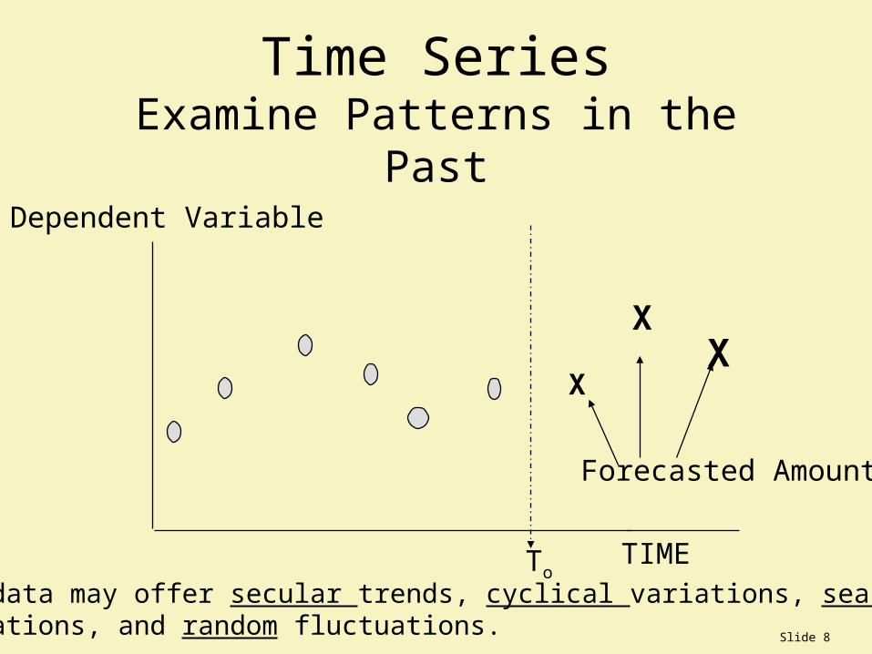
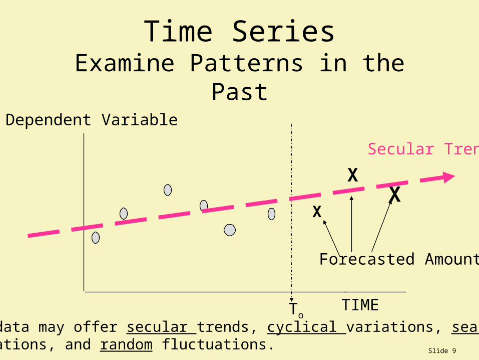
Time SeriesExamine Patterns in the Past

TIME

To

X

XX

Dependent Variable

Forecasted Amounts

The data may offer secular trends, cyclical variations, seasonalvariations, and random fluctuations.

Slide 9

Time SeriesExamine Patterns in the Past

TIME

To

X

XX

Dependent Variable

Secular Trend

Forecasted Amounts

The data may offer secular trends, cyclical variations, seasonalvariations, and random fluctuations.

Slide 10

Time SeriesExamine Patterns in the Past

TIME

To

X

XX

Dependent Variable

Secular TrendCyclical Variation

Forecasted Amounts

The data may offer secular trends, cyclical variations, seasonalvariations, and random fluctuations.

Slide 11

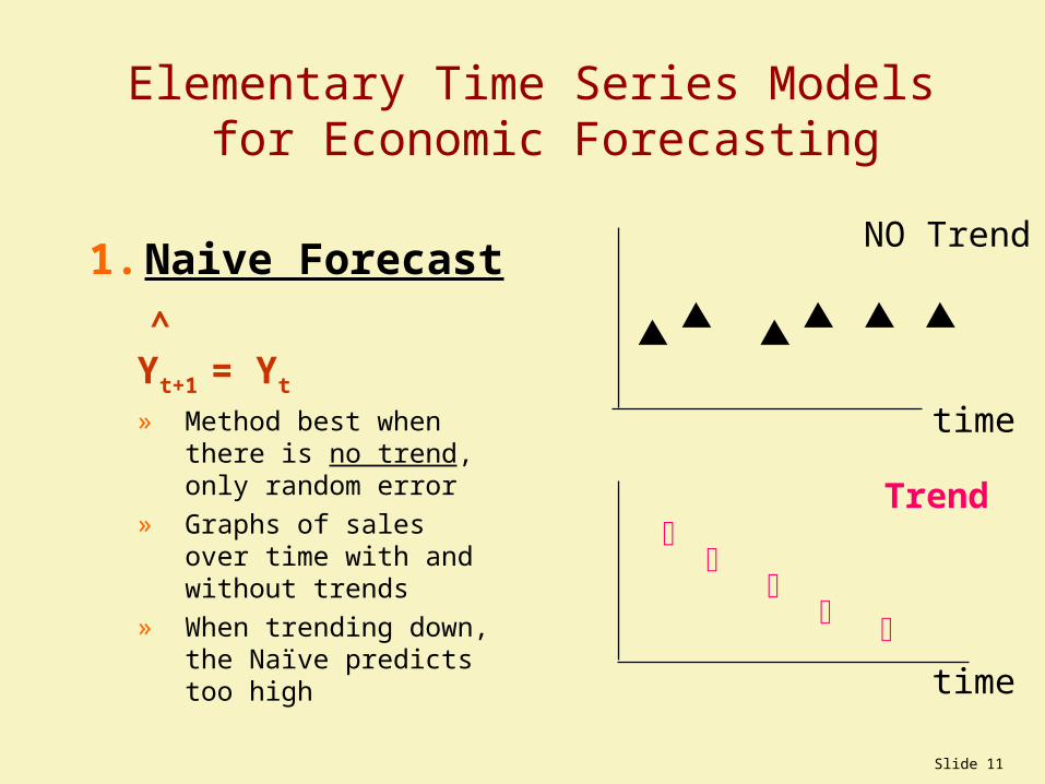
Elementary Time Series Models for Economic Forecasting

1. Naive Forecast

Yt+1 = Yt

» Method best when there is no trend, only random error

» Graphs of sales over time with and without trends

» When trending down, the Naïve predicts too high

NO Trend

Trend

^

time

time

Slide 12

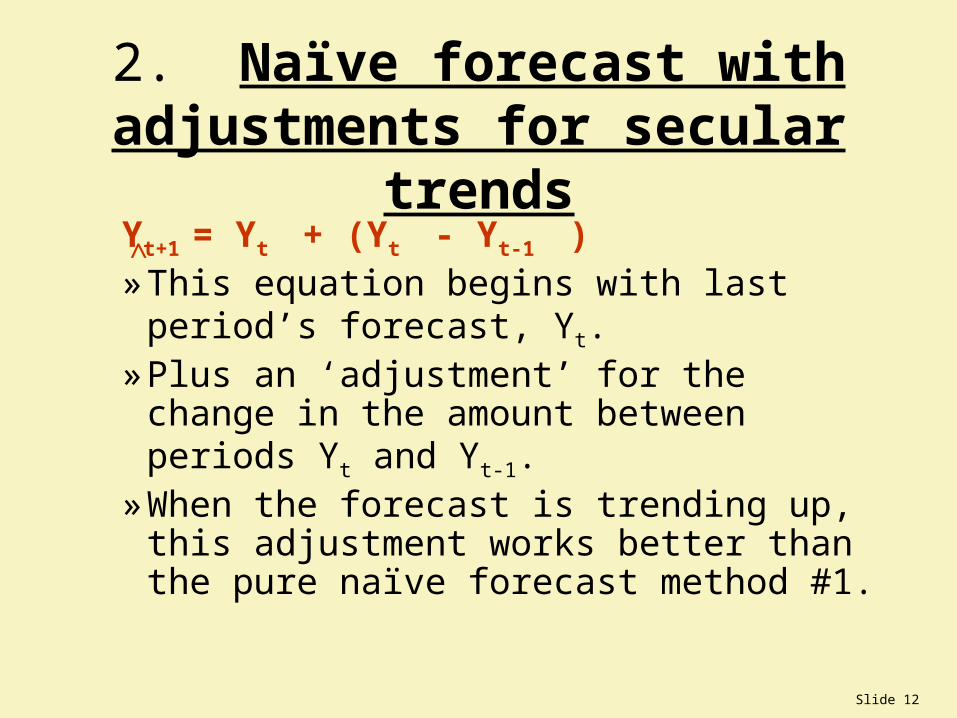
2. Naïve forecast with adjustments for secular trends

Yt+1 = Yt + (Yt - Yt-1 )» This equation begins with last period’s

forecast, Yt. » Plus an ‘adjustment’ for the change in the

amount between periods Yt and Yt-1.» When the forecast is trending up, this

adjustment works better than the pure naïve forecast method #1.

^

Slide 13

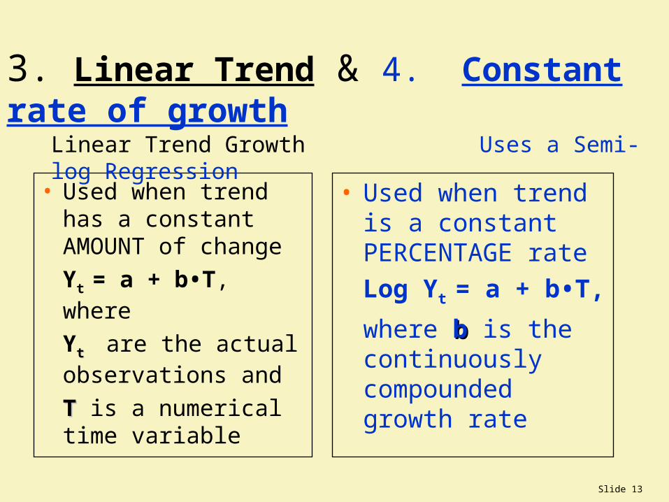
3. Linear Trend & 4. Constant rate of growth

• Used when trend has a constant AMOUNT of change

Yt = a + b•T, where

Yt t are the actual observations and

TT is a numerical time variable

• Used when trend is a constant PERCENTAGE rate

Log Yt = a + b•T,

where b b is the continuously compounded growth rate

Linear Trend Growth Uses a Semi-log Regression

Slide 14

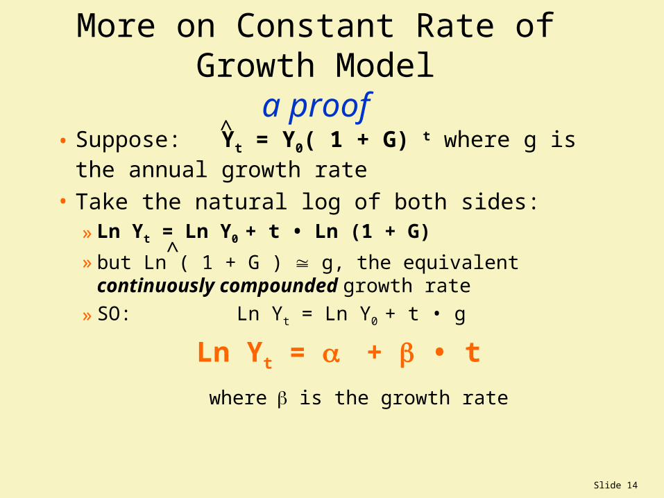
More on Constant Rate of Growth Modela proof

• Suppose: Yt = Y0( 1 + G) t where g is the annual growth rate

• Take the natural log of both sides:» Ln Yt = Ln Y0 + t • Ln (1 + G)

» but Ln ( 1 + G ) g, the equivalent continuously compounded growth rate

» SO: Ln Yt = Ln Y0 + t • g

Ln Yt = + • t

where is the growth rate

^

^

Slide 15

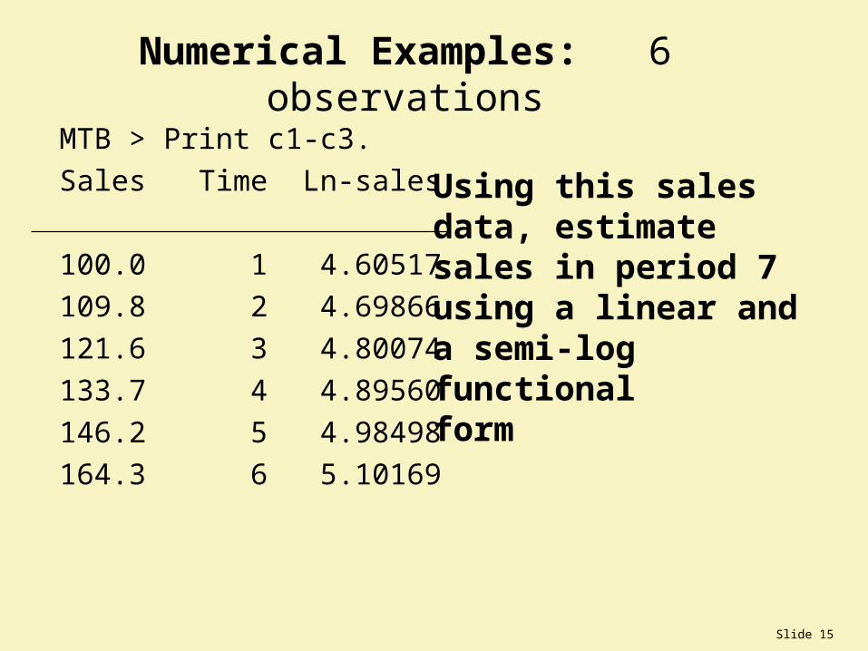
Numerical Examples: 6 observations

MTB > Print c1-c3.

Sales Time Ln-sales

100.0 1 4.60517

109.8 2 4.69866

121.6 3 4.80074

133.7 4 4.89560

146.2 5 4.98498

164.3 6 5.10169

Using this salesdata, estimate sales in period 7using a linear and a semi-log functionalform

Slide 16

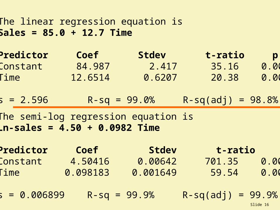
The linear regression equation isSales = 85.0 + 12.7 Time

Predictor Coef Stdev t-ratio pConstant 84.987 2.417 35.16 0.000Time 12.6514 0.6207 20.38 0.000

s = 2.596 R-sq = 99.0% R-sq(adj) = 98.8%

The semi-log regression equation isLn-sales = 4.50 + 0.0982 Time

Predictor Coef Stdev t-ratio pConstant 4.50416 0.00642 701.35 0.000Time 0.098183 0.001649 59.54 0.000

s = 0.006899 R-sq = 99.9% R-sq(adj) = 99.9%

Slide 17

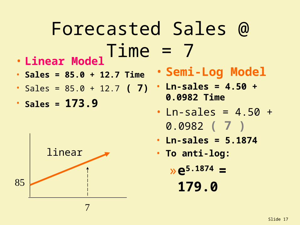
Forecasted Sales @ Time = 7• Linear Model• Sales = 85.0 + 12.7 Time

• Sales = 85.0 + 12.7 ( 7)

• Sales = 173.9

• Semi-Log Model• Ln-sales = 4.50 + 0.0982

Time

• Ln-sales = 4.50 + 0.0982 ( 7 )

• Ln-sales = 5.1874

• To anti-log:

» e5.1874 = 179.0

linear

Slide 18

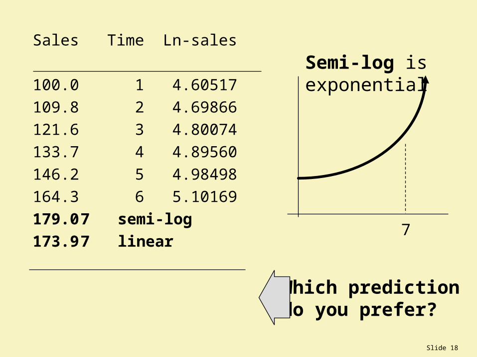
Sales Time Ln-sales

100.0 1 4.60517

109.8 2 4.69866

121.6 3 4.80074

133.7 4 4.89560

146.2 5 4.98498

164.3 6 5.10169

179.0 7 semi-log

173.9 7 linearWhich prediction do you prefer?

Semi-log isexponential

7

Slide 19

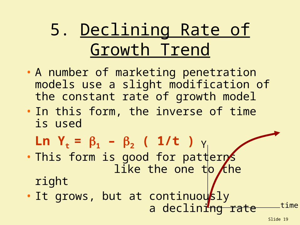
5. Declining Rate of Growth Trend

• A number of marketing penetration models use a slight modification of the constant rate of growth model

• In this form, the inverse of time is used

Ln Yt = 1 – 2 ( 1/t )• This form is good for patterns

like the one to the right• It grows, but at continuously

a declining rate time

Y

Slide 20

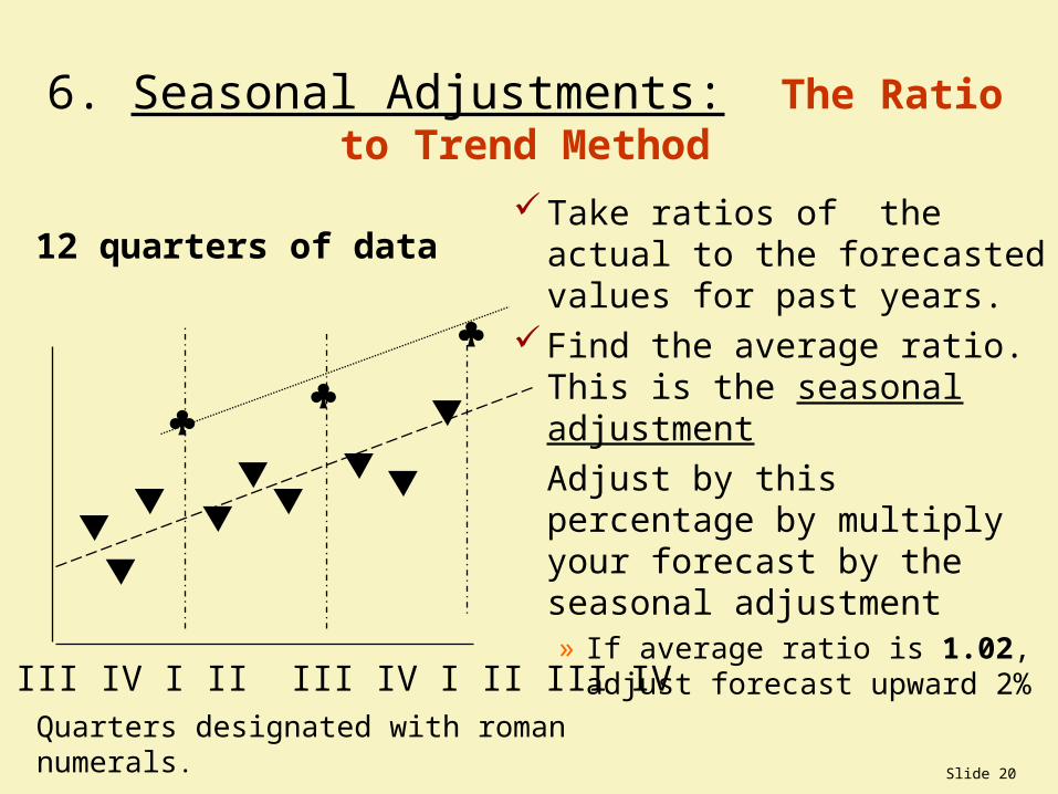
6. Seasonal Adjustments: The Ratio to Trend Method

Take ratios of the actual to the forecasted values for past years.

Find the average ratio. This is the seasonal adjustment

Adjust by this percentage by multiply your forecast by the seasonal adjustment» If average ratio is 1.02, adjust

forecast upward 2%

12 quarters of data

I II III IV I II III IV I II III IV

Quarters designated with roman numerals.

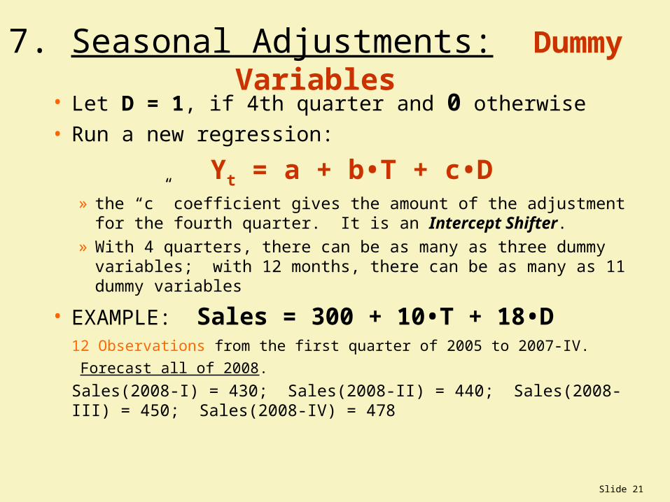
Slide 21

• Let D = 1, if 4th quarter and 0 otherwise

• Run a new regression:

Yt = a + b•T + c•D » the “c” coefficient gives the amount of the adjustment for the fourth

quarter. It is an Intercept Shifter.» With 4 quarters, there can be as many as three dummy variables; with 12

months, there can be as many as 11 dummy variables

• EXAMPLE: Sales = 300 + 10•T + 18•D12 Observations from the first quarter of 2005 to 2007-IV.

Forecast all of 2008.

Sales(2008-I) = 430; Sales(2008-II) = 440; Sales(2008-III) = 450; Sales(2008-IV) = 478

7. Seasonal Adjustments: Dummy Variables

Slide 22

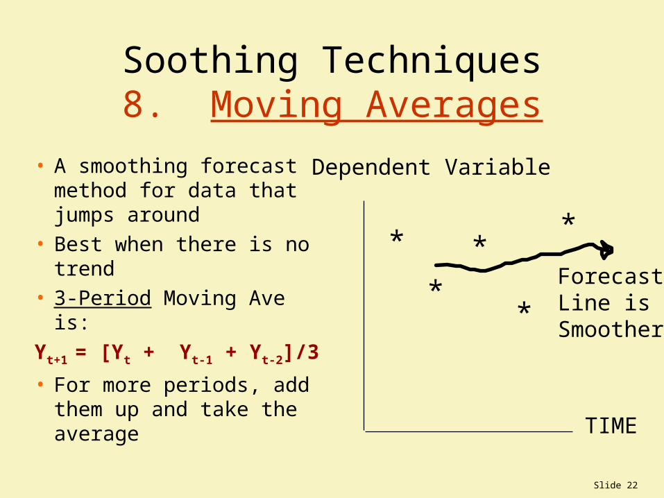
Soothing Techniques8. Moving Averages

• A smoothing forecast method for data that jumps around

• Best when there is no trend• 3-Period Moving Ave is:

Yt+1 = [Yt + Yt-1 + Yt-2]/3

• For more periods, add them up and take the average

*

*

*

*

*

ForecastLine isSmoother

TIME

Dependent Variable

Slide 23

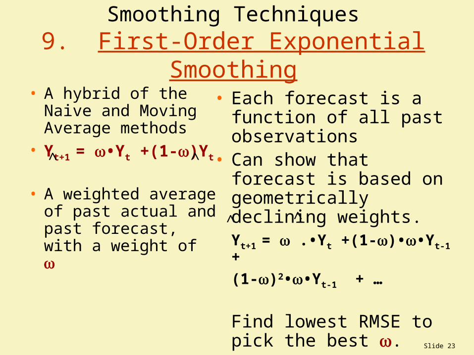
Smoothing Techniques9. First-Order Exponential Smoothing

• A hybrid of the Naive and Moving Average methods

• Yt+1 = •Yt +(1-)Yt

• A weighted average of past actual and past forecast, with a weight of

• Each forecast is a function of all past observations

• Can show that forecast is based on geometrically declining weights.Yt+1 = .•Yt +(1-)••Yt-1 +

(1-)2••Yt-1 + …

Find lowest RMSE to pick the best .

^ ^

^ ^

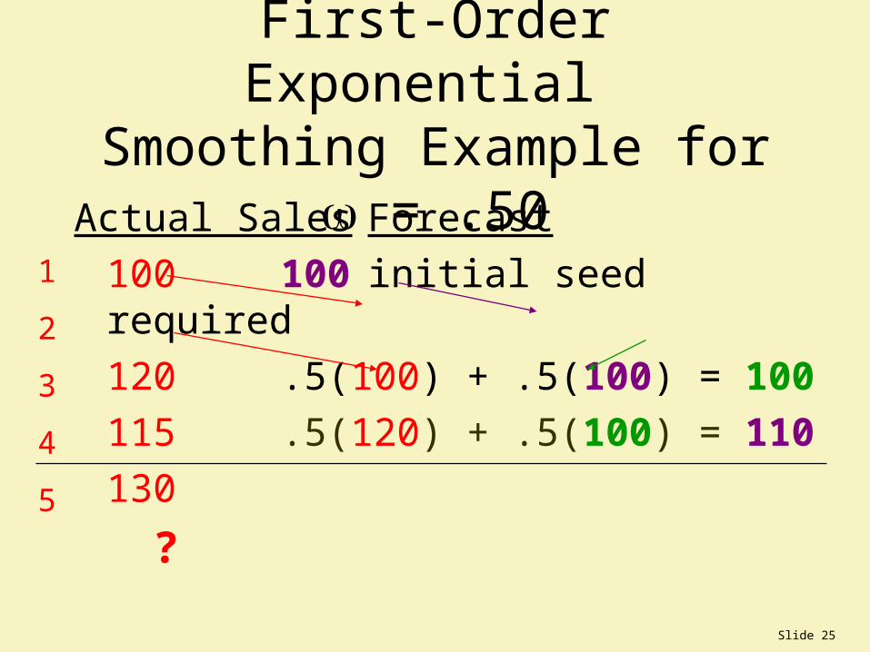
Slide 24

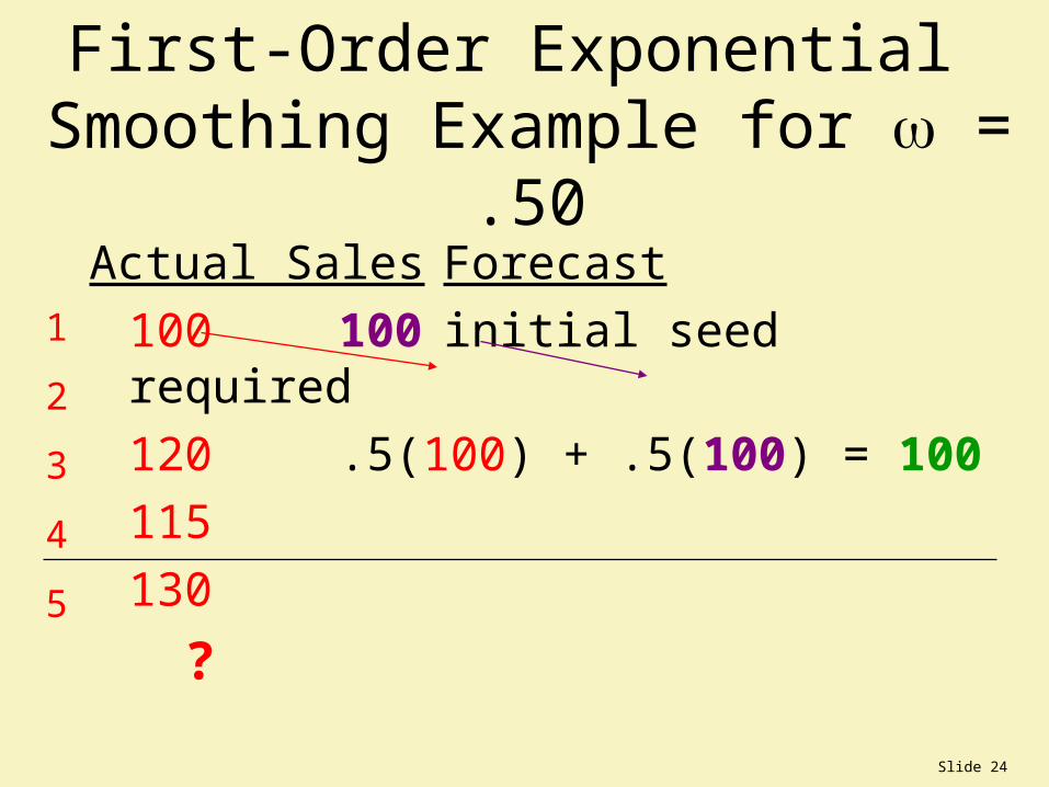
First-Order Exponential Smoothing Example for = .50

Actual Sales Forecast

100 100 initial seed required

120 .5(100) + .5(100) = 100

115

130

?

1

2

3

4

5

Slide 25

First-Order Exponential Smoothing Example for = .50

Actual Sales Forecast

100 100 initial seed required

120 .5(100) + .5(100) = 100

115 .5(120) + .5(100) = 110

130

?

1

2

3

4

5

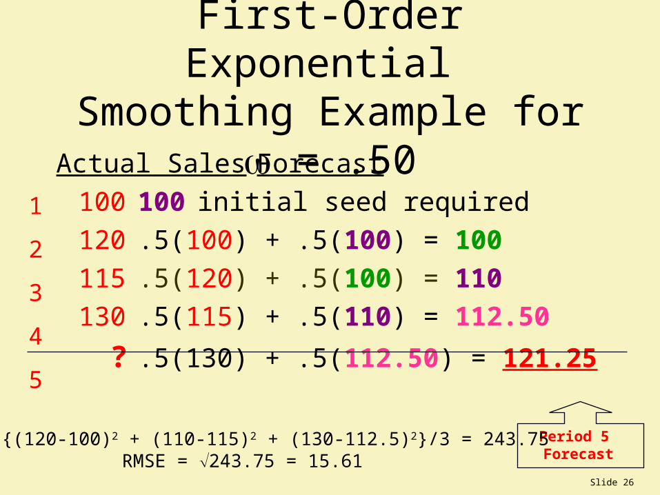
Slide 26

First-Order Exponential Smoothing Example for = .50

Actual Sales Forecast

100 100 initial seed required

120 .5(100) + .5(100) = 100

115 .5(120) + .5(100) = 110

130 .5(115) + .5(110) = 112.50

? .5(130) + .5(112.50) = 121.25

Period 5 Forecast

MSE = {(120-100)2 + (110-115)2 + (130-112.5)2}/3 = 243.75RMSE = 243.75 = 15.61

1

2

3

4

5

Slide 27

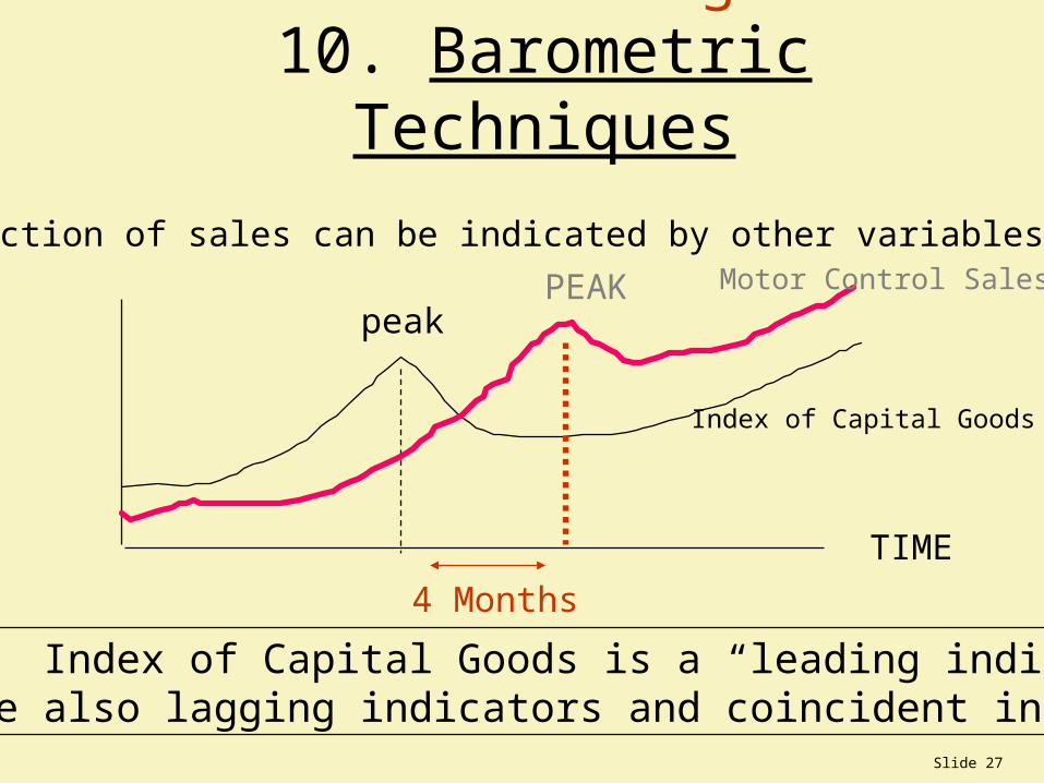
Direction of sales can be indicated by other variables.

TIME

Index of Capital Goods

peakPEAK Motor Control Sales

4 Months

Example: Index of Capital Goods is a “leading indicator”There are also lagging indicators and coincident indicators

Qualitative Forecasting10. Barometric Techniques

Slide 28

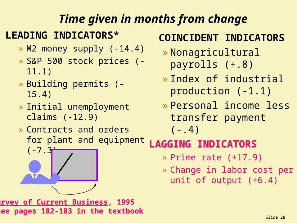
LEADING INDICATORS*» M2 money supply (-14.4)

» S&P 500 stock prices (-11.1)

» Building permits (-15.4)

» Initial unemployment claims (-12.9)

» Contracts and orders for plant and equipment (-7.3)

COINCIDENT INDICATORS» Nonagricultural payrolls

(+.8)» Index of industrial

production (-1.1)» Personal income less

transfer payment (-.4)

LAGGING INDICATORS» Prime rate (+17.9)

» Change in labor cost per unit of output (+6.4)

*Survey of Current Business, 1995 See pages 182-183 in the textbook

Time given in months from change

Slide 29

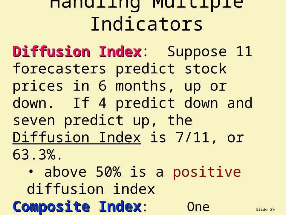
Handling Multiple IndicatorsDiffusion IndexDiffusion Index: Suppose 11 forecasters predict stock prices in 6 months, up or down. If 4 predict down and seven predict up, the Diffusion Index is 7/11, or 63.3%.

• above 50% is a positive diffusion index

Composite IndexComposite Index: One indicator rises 4% and another rises 6%. Therefore, the Composite Index is a 5% increase.

• used for quantitative forecasting

Slide 30

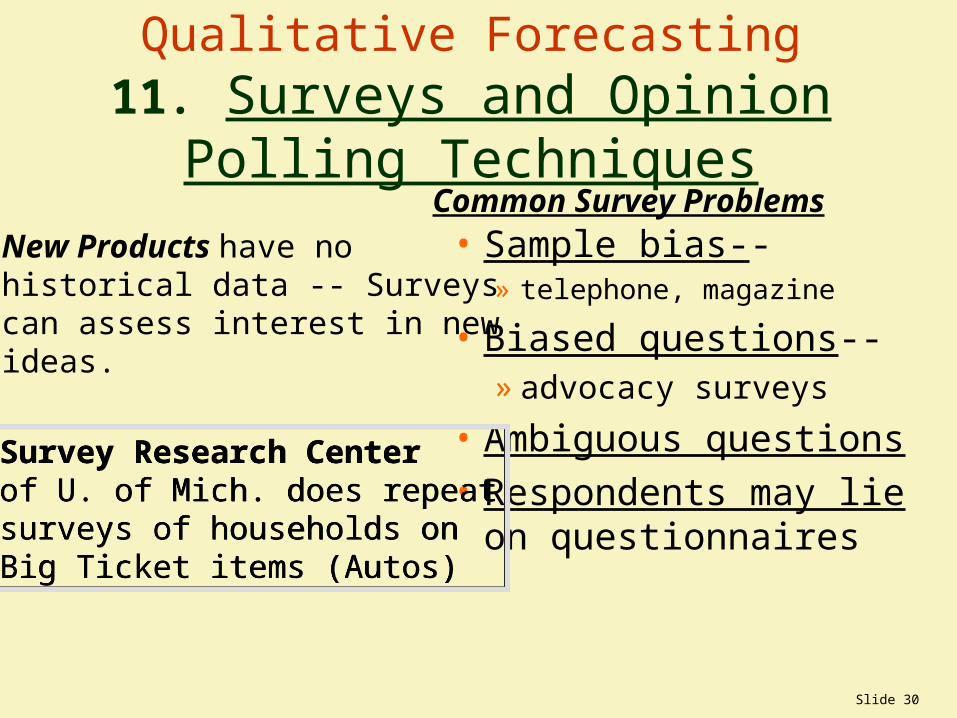
Qualitative Forecasting11. Surveys and Opinion Polling Techniques

• Sample bias--» telephone, magazine

• Biased questions--» advocacy surveys

• Ambiguous questions

• Respondents may lie on questionnaires

New Products have nohistorical data -- Surveyscan assess interest in newideas.

Survey Research Centerof U. of Mich. does repeatsurveys of households onBig Ticket items (Autos)

Survey Research Centerof U. of Mich. does repeatsurveys of households onBig Ticket items (Autos)

Common Survey Problems

Slide 31

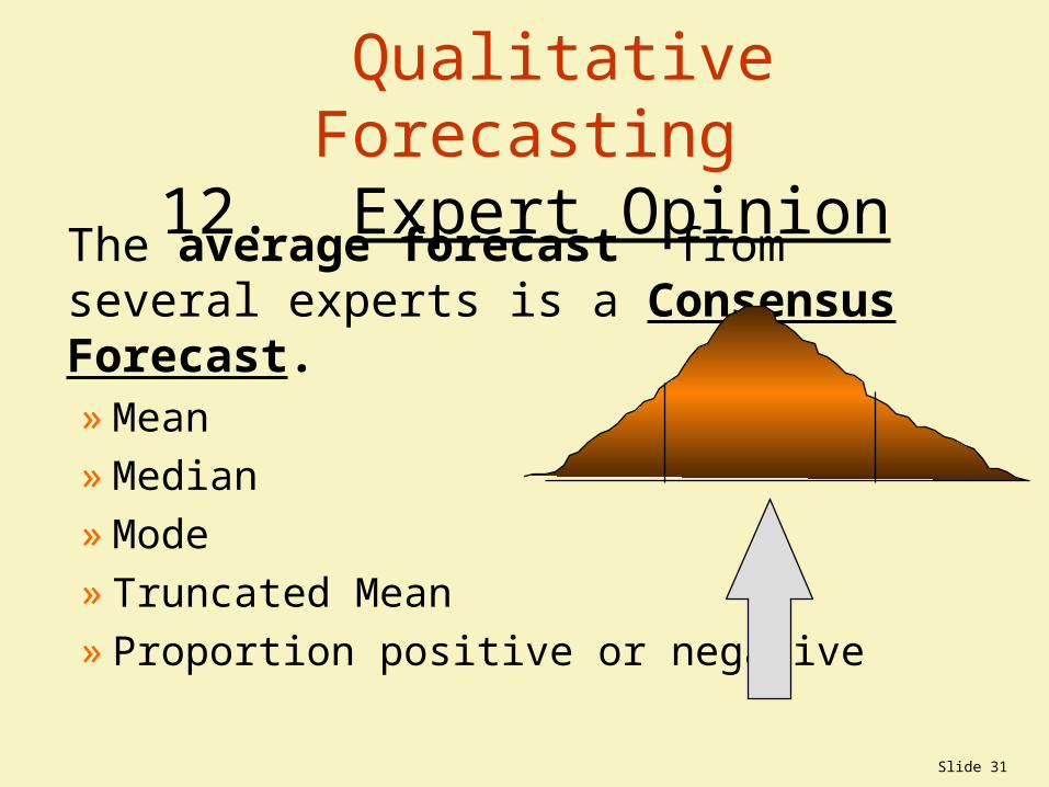
Qualitative Forecasting12. Expert Opinion

The average forecast from several experts is a Consensus Forecast.» Mean» Median» Mode» Truncated Mean» Proportion positive or negative

Slide 32

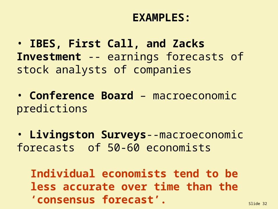
EXAMPLES:

• IBES, First Call, and Zacks Investment -- earnings forecasts of stock analysts of companies

• Conference Board – macroeconomic predictions

• Livingston Surveys--macroeconomic forecasts of 50-60 economists

Individual economists tend to be less accurate over time than the ‘consensus forecast’.

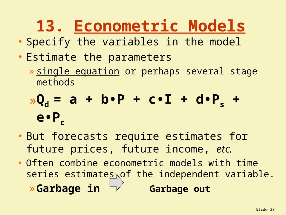
Slide 33

13. Econometric Models• Specify the variables in the model

• Estimate the parameters » single equation or perhaps several stage methods

»Qd = a + b•P + c•I + d•Ps + e•Pc

• But forecasts require estimates for future prices, future income, etc.

• Often combine econometric models with time series estimates of the independent variable.

» Garbage in Garbage out

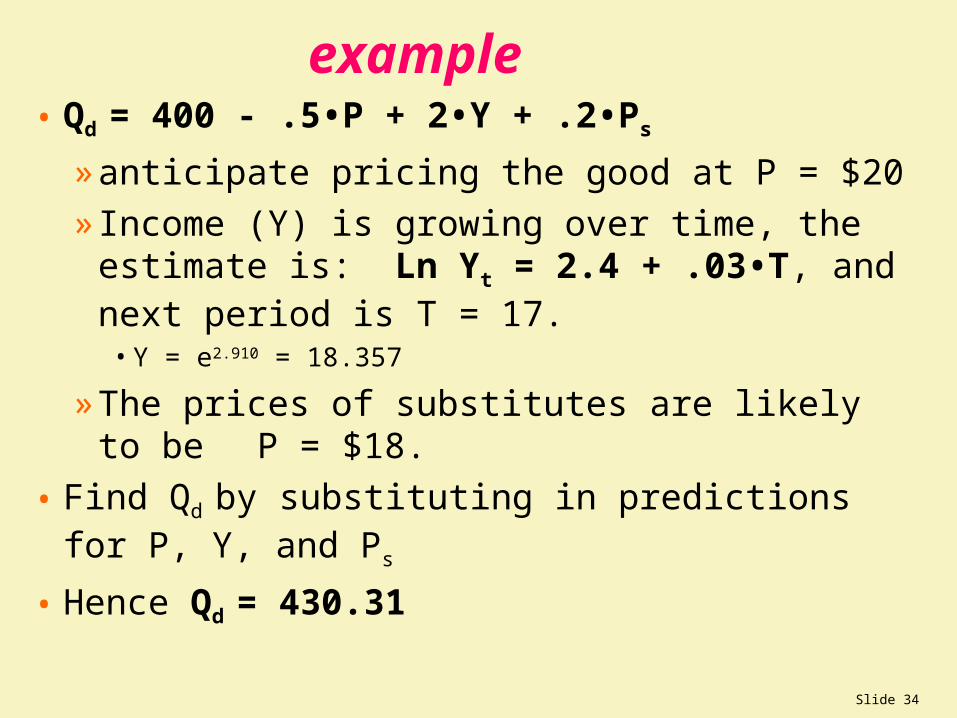
Slide 34

example • Qd = 400 - .5•P + 2•Y + .2•Ps

» anticipate pricing the good at P = $20

» Income (Y) is growing over time, the estimate is: Ln Yt = 2.4 + .03•T, and next period is T = 17.

• Y = e2.910 = 18.357

» The prices of substitutes are likely to be P = $18.

• Find Qd by substituting in predictions for P, Y, and Ps

• Hence Qd = 430.31

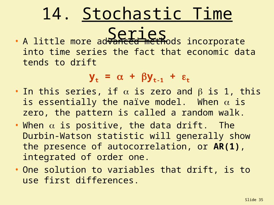
Slide 35

14. Stochastic Time Series• A little more advanced methods incorporate into time

series the fact that economic data tends to drift

yt = + yt-1 + t

• In this series, if is zero and is 1, this is essentially the naïve model. When is zero, the pattern is called a random walk.

• When is positive, the data drift. The Durbin-Watson statistic will generally show the presence of autocorrelation, or AR(1), integrated of order one.

• One solution to variables that drift, is to use first differences.

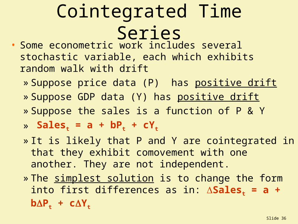
Slide 36

Cointegrated Time Series• Some econometric work includes several stochastic

variable, each which exhibits random walk with drift» Suppose price data (P) has positive drift» Suppose GDP data (Y) has positive drift» Suppose the sales is a function of P & Y

» Salest = a + bPt + cYt

» It is likely that P and Y are cointegrated in that they exhibit comovement with one another. They are not independent.

» The simplest solution is to change the form into first differences as in: Salest = a + bPt + cYt