Embed Size (px)
Citation preview

Slide # 1
STANDARD COSTING & VARIANCE ANALYSIS
KHALID AZIZKHALID AZIZ0322-33857520322-33857520312-23028700312-2302870
FRESH CLASSES MA-ECONOMICS 15FRESH CLASSES MA-ECONOMICS 15THTH FEBRUARY 2010FEBRUARY 2010

Slide # 2
JOIN KHALID AZIZ
• ECONOMICS OF ICMAP, ICAP, MA-ECONOMICS, B.COM.
• FINANCIAL ACCOUNTING OF ICMAP STAGE 1,3,4 ICAP MODULE B, B.COM, BBA, MBA & PIPFA.
• COST ACCOUNTING OF ICMAP STAGE 2,3 ICAP MODULE D, BBA, MBA & PIPFA.
• CONTACT:• 0322-3385752• R-1173,ALNOOR SOCIETY, BLOCK 19,F.B.AREA,
KARACHI, PAKISTAN.

Slide # 3
Standard Costs & Variance Analysis
Learning objectives
• Q1: How are standard costs established?
• Q2: What is variance analysis and how is it performed?
• Q3: How are direct cost variances calculated?
• Q4: How is direct cost variance information analyzed and used?
• Q5: How are variable and fixed overhead variances calculated?
• Q6: How is overhead variance information analyzed and used?
• Q7: How are manufacturing cost variances closed?
• Q8: Which profit-related variances are commonly analyzed?

Slide # 4
Q1: Standard Costs
• Organizations set standards to help plan operations.
• A standard cost is the expected cost of providing a good or service.
• In manufacturing, the standard cost of a unit of output is comprised of:• the standard price (SP) of the input, and • the standard quantity of the input expected
to be consumed in the production of one output unit.

Slide # 5
Q1: Establishing & Using Standard Costs
• Standards can be set using:• Information from the prior year• Engineered estimates• New information available
• Standards can be used for:• Planning future operations• Monitoring current operations• Motivating manager and employee behavior• Evaluating performance

Slide # 6
Q2: Standard Cost Variances
• The difference between an actual cost and the standard cost of producing goods or services at the actual volume level is called a standard cost variance.
• Managers investigate the reasons for standard cost variances so that:• efficiencies can be rewarded and replicated,• inefficiencies can be minimized, and• the validity of the standards can be assessed.

Slide # 7
Q3: Direct Cost Variances
• A price variance is the difference between the standard cost of resources purchased (or that should have been consumed) and the actual cost.
• An efficiency variance measures whether inputs were used efficiently.• It is the difference between the inputs used
and the inputs that should have been used, times the standard price of the input

Slide # 8
Q3: Direct Labor Cost Variances
• The direct labor price and efficiency variances are a decomposition of the direct labor flexible budget variance.
• The year-end flexible budget direct labor cost is based on the standard direct labor hours for the actual output, or standard quantity allowed (SQA).
• Other abbreviations used:• SP = standard price of the input• AP = actual price of the input• AQ = actual quantity of the input used

Slide # 9
Q3: Direct Labor Cost Variances
The direct labor price and efficiency variances are a decomposition of the direct labor flexible budget variance.
The direct labor price and efficiency variances are a decomposition of the direct labor flexible budget variance.
SQA x SP
Year-end flexible budget
Year-end actual results
AQ x APAQ x SP
DL flexible budget variance
DL price varianceDL efficiency variance
DLPV = [SP – AP] x AQDLEV = [SQA – AQ] x SP
Slide # 10
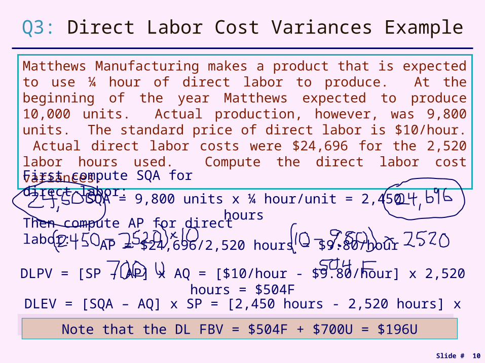
Matthews Manufacturing makes a product that is expected to use ¼ hour of direct labor to produce. At the beginning of the year Matthews expected to produce 10,000 units. Actual production, however, was 9,800 units. The standard price of direct labor is $10/hour. Actual direct labor costs were $24,696 for the 2,520 labor hours used. Compute the direct labor cost variances.
Q3: Direct Labor Cost Variances Example
First compute SQA for direct labor:
SQA = 9,800 units x ¼ hour/unit = 2,450 hours
DLPV = [SP – AP] x AQ = [$10/hour - $9.80/hour] x 2,520 hours = $504F
Then compute AP for direct labor:
AP = $24,696/2,520 hours = $9.80/hour
DLEV = [SQA – AQ] x SP = [2,450 hours - 2,520 hours] x $10/hour = $700U
Note that the DL FBV = $504F + $700U = $196UNote that the DL FBV = $504F + $700U = $196U

Slide # 11
What are some possible explanations for the direct labor cost variances of Matthews Manufacturing?
Q4: Direct Labor Cost Variances Example
• The favorable price variance could be due to:
• an incorrect standard price,
• using a higher percentage of lower-paid workers than expected, or
• a favorable renegotiation of a labor contract.
• The unfavorable efficiency variance could be due to:
• an incorrect standard quantity for labor,
• inefficiency of direct labor personnel,
• unexpected problems with machinery, or
• lower quality of inputs that were more difficult to use.

Slide # 12
Q3: Direct Material Cost Variances
• The direct materials and direct labor efficiency variances are computed in the same fashion.
• The direct material price variance is computed slightly differently than the direct labor price variance.
• Direct materials can be purchased and stored, and direct labor is consumed as it is purchased.
• The direct materials price and efficiency variances do not sum to the direct material flexible budget variance when there are any direct materials inventories.

Slide # 13
Q3: Direct Material Cost Variances
The direct material price variance is based on the actual quantity of direct materials purchased, not the actual quantity of direct materials used.
The direct material price variance is based on the actual quantity of direct materials purchased, not the actual quantity of direct materials used.
SQA x SP
Year-end flexible budget
AQ x SP
DM price variance
DM efficiency variance
DMPV = [SP – AP] x Actual Quantity Purchased
DMEV = [SQA – AQ] x SP
Actual Quantity Purchased x SP
Actual Quantity Purchased x AP
Remember that AQ=Actual quantity
used, not actual quantity purchased.
Remember that AQ=Actual quantity
used, not actual quantity purchased.

Slide # 14
Matthews Manufacturing makes a product that is expected to use 2 pounds of direct material to produce. At the beginning of the year Matthews expected to produce 10,000 units. Actual production, however, was 9,800 units. The standard price of direct materials is $3/pound. Matthews purchased 20,500 pounds of direct material at $3.10/pound, and used 19,400 pounds. Compute the direct material cost variances.
Q3: Direct Material Cost Variances Example
First compute SQA for direct materials:
SQA = 9,800 units x 2 pounds/unit = 19,600 pounds
DMPV = [SP – AP] x Actual Quantity Purchased =
[$3/pound - $3.10/pound] x 20,500 pounds = $2,050U
DMEV = [SQA – AQ] x SP =
[19,600 pounds - 19,400 pounds] x $3/pound = $600F

Slide # 15
What are some possible explanations for the direct material cost variances of Matthews Manufacturing?
Q4: Direct Material Cost Variances Example
• The unfavorable price variance could be due to:
• an incorrect standard price,
• an unexpected price increase from a supplier, or
• the purchase of higher quality materials.
• The favorable efficiency variance could be due to:
• an incorrect standard quantity for material,
• efficient use of direct materials during production, or
• less waste of direct materials due to higher material quality.

Slide # 16
JOIN KHALID AZIZ
• ECONOMICS OF ICMAP, ICAP, MA-ECONOMICS, B.COM.
• FINANCIAL ACCOUNTING OF ICMAP STAGE 1,3,4 ICAP MODULE B, B.COM, BBA, MBA & PIPFA.
• COST ACCOUNTING OF ICMAP STAGE 2,3 ICAP MODULE D, BBA, MBA & PIPFA.
• CONTACT:• 0322-3385752• R-1173,ALNOOR SOCIETY, BLOCK 19,F.B.AREA,
KARACHI, PAKISTAN.

Slide # 17
• The direct material price variance is recorded when the materials are purchased.
• The direct material efficiency variance is recorded when the materials are used in production.
• The direct labor price and efficiency variances are recorded when labor is used in production.
• Work in process inventory is debited for the standard cost of the inputs that should have been used to produce the actual quantity of outputs (SP x SQA).
Q3: Recording Direct Cost Variances

Slide # 18
The journal entry to record the use of direct labor is:The journal entry to record the use of direct labor is:
Q3: Recording Direct Labor Cost Variances
dr. Work in process inventory SP x SQA
dr. or cr. DLEV [SQA-AQ] x SP
dr. or cr. DLPV [SP-AP] x AQ
cr. Accrued payroll AP x AQ
Unfavorable variances are debited to the variance accounts and favorable variances
are credited to the variance accounts.
Unfavorable variances are debited to the variance accounts and favorable variances
are credited to the variance accounts.
Slide # 19
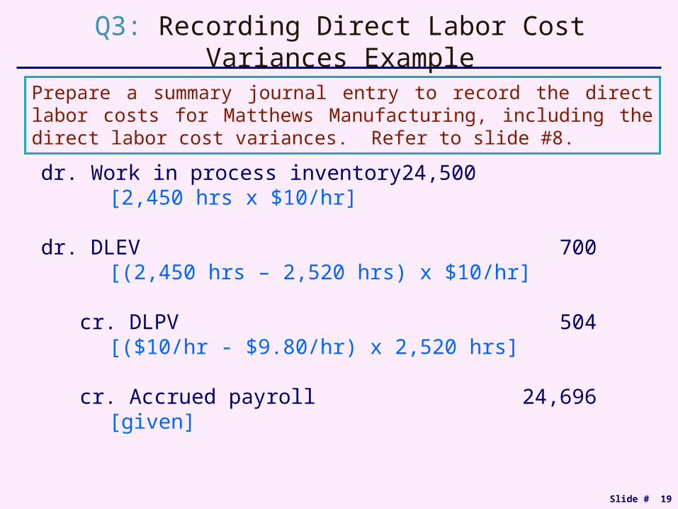
Prepare a summary journal entry to record the direct labor costs for Matthews Manufacturing, including the direct labor cost variances. Refer to slide #8.
Q3: Recording Direct Labor CostVariances Example
dr. Work in process inventory 24,500[2,450 hrs x $10/hr]
dr. DLEV 700[(2,450 hrs – 2,520 hrs) x $10/hr]
cr. DLPV 504[($10/hr - $9.80/hr) x 2,520 hrs]
cr. Accrued payroll 24,696[given]
Slide # 20
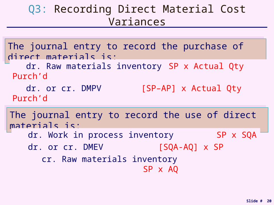
The journal entry to record the purchase of direct materials is:The journal entry to record the purchase of direct materials is:
Q3: Recording Direct Material Cost Variances
dr. Raw materials inventory SP x Actual Qty Purch’d
dr. or cr. DMPV [SP–AP] x Actual Qty Purch’d
cr. Accounts payable AP x Actual Qty Purch’d
The journal entry to record the use of direct materials is:The journal entry to record the use of direct materials is:
dr. Work in process inventory SP x SQA
dr. or cr. DMEV [SQA-AQ] x SP
cr. Raw materials inventory SP x AQ

Slide # 21
The journal entry to record the purchase of direct materials is:
Q3: Recording Direct Material CostVariances Example
dr. Raw materials inventory [$3/lb x 20,500 lbs] 61,500dr. DMPV [($3/lb –$3.10/lb) x 20,500 lbs] 2,050
cr. Accounts payable [$3.10/lb x 20,500 lbs] 63,550
The journal entry to record the use of direct materials is:
dr. Work in process inventory [$3/lb X 19,600 lbs] 58,800cr. DMEV [(19,600 lbs – 19,400 lbs) x $3/lb] 600cr. Raw materials inventory [19,400 lbs x $3/lb] 58,200
Prepare summary journal entries to record the purchase and the use of direct material for Matthews Manufacturing, including the direct material cost variances. Refer to slide #12.

Slide # 22
Q5: Allocating Overhead Costs
• Chapter 5 covered the allocation of overhead to units of production.
• Estimated overhead rates are calculated for both fixed and variable overhead.
Standard variable
overhead allocation rate
Estimated variable overhead costsEstimated volume of an overhead allocation base
=
Standard fixed overhead
allocation rate
Estimated fixed overhead costsEstimated volume of an overhead allocation base
=

Slide # 23
Q5: Overhead Cost Management
• For both variable and fixed overhead, cost management includes reducing non-value-added costs.
• For each variable overhead cost pool, cost management includes reducing the consumption of the related cost allocation base.
• For fixed overhead, cost management involves a trade-off between insufficient and excess capacity.

Slide # 24
Q5: Variable Overhead Cost Variances
• The variable overhead cost variances are computed in the same fashion as the direct labor cost variances.
• The variable overhead spending variance is similar to the direct labor price variance.
• The variable overhead efficiency variance is similar to the direct labor efficiency variance.
• The variable overhead (flexible) budget variance is the sum of these two variable overhead variances.

Slide # 25
Q5: Variable Overhead Cost Variances
The standard quantity allowed (SQA) in the variable overhead cost variance calculations is the quantity of the variable overhead allocation base that should have been used to produce the actual output. SR is the standard variable overhead allocation rate.
The standard quantity allowed (SQA) in the variable overhead cost variance calculations is the quantity of the variable overhead allocation base that should have been used to produce the actual output. SR is the standard variable overhead allocation rate.
SQA x SR
Year-end flexible budget
Year-end actual results
Total actual VOAQ x SR
VO flexible budget variance
VO spending varianceVO efficiency variance
VOSV = [AQ x SR] – actual VOVOEV = [SQA – AQ] x SR

Slide # 26
Matthews Manufacturing makes a product that is expected to use ¼ hour of direct labor to produce. At the beginning of the year Matthews expected to produce 10,000 units. Actual production, however, was 9,800 units. The estimated variable overhead allocation rate is $4 per direct labor hour, actual variable overhead costs were $10,450, and actual direct labor hours were 2,520. Compute the variable overhead cost variances.
Q5: Variable Overhead Cost Variances Example
First compute SQA for direct labor, the VO cost allocation base:
SQA = 9,800 units x ¼ hour/unit = 2,450 hours
VOSV = AQ x SR – actual VO = 2,520 hrs x $4/hr - $10,450 = $370U
VOEV = [SQA – AQ] x SR = [2,450 hours - 2,520 hours] x $4/hour = $280U
Note that the VO FBV = $280U + $370U = $650UNote that the VO FBV = $280U + $370U = $650U

Slide # 27
What are some possible explanations for the variable overhead cost variances of Matthews Manufacturing?
Q6: Variable Overhead Cost Variances Example
• The favorable spending variance could be due to:
• an incorrect standard variable overhead rate per direct labor hour,
• lower prices than expected for the components of the variable overhead cost pool (e.g. a lower price per quart of machine oil), or
• lower consumption than expected of the components of the variable overhead cost pool (e.g. less indirect labor used per direct labor hour).
• The unfavorable efficiency variance could be due to:
• an incorrect standard quantity for labor,
• inefficiency of direct labor personnel,
• unexpected problems with machinery, or
• lower quality of inputs that were more difficult to use.
Slide # 28
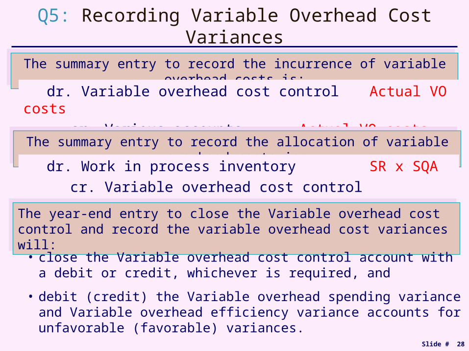
The summary entry to record the incurrence of variable overhead costs is:The summary entry to record the incurrence of variable overhead costs is:
Q5: Recording Variable Overhead Cost Variances
dr. Variable overhead cost control Actual VO costs
cr. Various accounts Actual VO costs
The summary entry to record the allocation of variable overhead costs is:The summary entry to record the allocation of variable overhead costs is:
dr. Work in process inventory SR x SQA
cr. Variable overhead cost control SR x SQA
The year-end entry to close the Variable overhead cost control and record the variable overhead cost variances will:The year-end entry to close the Variable overhead cost control and record the variable overhead cost variances will:
• close the Variable overhead cost control account with a debit or credit, whichever is required, and
• debit (credit) the Variable overhead spending variance and Variable overhead efficiency variance accounts for unfavorable (favorable) variances.

Slide # 29
The journal entry to record the incurrence of variable overhead costs is:
Q3: Recording Variable Overhead CostVariances Example
dr. Variable overhead cost control 10,450cr. Various accounts 10,450
The journal entry to record the allocation of variable overhead is:
dr. Work in process inventory [$4/hr X 2,450 hrs] 9,800cr. Variable overhead cost control 9,800
Prepare summary journal entries to record the incurrence of and the allocation to work in process of variable overhead costs for Matthews Manufacturing. Also prepare the year-end entry to close variable overhead control and record the variances. Refer to slide #22.
The year-end entry to close the Variable overhead cost control account is:
dr. VOSV 280dr. VOEV 370
cr. Variable overhead cost control 650

Slide # 30
Q5: Fixed Overhead Cost Variances
• The fixed overhead spending variance is the same as the fixed overhead (flexible) budget variance.
• There is no fixed overhead efficiency variance because changes in the quantity of the fixed overhead allocation base do not cause changes in actual total fixed overhead costs.
• The production volume variance occurs when actual volume is different than the static budget estimated volume.

Slide # 31
Q5: The Production Volume Variance
• Allocating fixed overhead to production using a standard rate per unit of a cost allocation base treats fixed overhead as a variable cost for bookkeeping purposes.
• Since fixed overhead is not a variable cost, the fixed overhead allocated to production will differ from budgeted fixed overhead when actual volume differs from static budget estimated volume.
• The production volume variance is favorable (unfavorable) when actual volume exceeds (is less than) static budget estimated volume.

Slide # 32
Q5: Fixed Overhead Cost Variances
The standard quantity allowed (SQA) in the fixed overhead cost variance calculations is the quantity of the fixed overhead allocation base that should have been used to produce the actual output. SR is the standard fixed overhead allocation rate.
The standard quantity allowed (SQA) in the fixed overhead cost variance calculations is the quantity of the fixed overhead allocation base that should have been used to produce the actual output. SR is the standard fixed overhead allocation rate.
Total FO budget variance
FO spending varianceFO production volume variance
FOPVV = [SQA x SR] – estimated FO
SQA x SR
Static & year-end budget
Year-end actual results
Total actual FOEstimated FO
Allocated fixed overhead
FOSV =Estimated FO – actual FO

Slide # 33
Matthews Manufacturing makes a product that is expected to use 1.2 machine hours to produce. At the beginning of the year Matthews expected to produce 10,000 units. Actual production, however, was 9,800 units. Estimated fixed overhead at the beginning of the year was $60,000 and actual fixed overhead was $58,100. Actual machine hours for the year totaled 12,200 hours. Compute the fixed overhead cost variances.
Q5: Fixed Overhead Cost Variances Example
First compute SQA for machine hours:
SQA = 9,800 units x 1.2 hours/unit = 11,760 hours
FOSV = Estimated FO – actual FO = $60,000 - $58,100 = $1,900F
FOPVV = SQA x SR – estimated FO =
11,760 hours x $5/hr - $60,000 = $1,200U
Next compute the estimated fixed overhead rate per machine hour:
SR = $60,000/[10,000 units x 1.2 hrs/unit] = $5/hr

Slide # 34
What are some possible explanations for the fixed overhead cost variances of Matthews Manufacturing?
Q6: Fixed Overhead Cost Variances Example
• The favorable spending variance could be due to:
• an incorrect estimate for fixed overhead costs,
• a decision to forgo a budgeted discretionary fixed cost, or
• a favorable renegotiation of leasing agreements.
• The unfavorable production volume variance is due to:
• an actual volume level that is less than the static budget volume level.

Slide # 35
The summary entry to record the incurrence of fixed overhead costs is:The summary entry to record the incurrence of fixed overhead costs is:
Q5: Recording Fixed Overhead Cost Variances
dr. Fixed overhead cost control Actual FO costs
cr. Various accounts Actual FO costs
The summary entry to record the allocation of fixed overhead costs is:The summary entry to record the allocation of fixed overhead costs is:
dr. Work in process inventory SR x SQA
cr. Fixed overhead cost control SR x SQA
The year-end entry to close the fixed overhead cost control and record the fixed overhead cost variances will:The year-end entry to close the fixed overhead cost control and record the fixed overhead cost variances will:
• close the Fixed overhead cost control account with a debit or credit, whichever is required, and
• debit (credit) the fixed overhead production volume variance and fixed overhead spending variance accounts for unfavorable (favorable) variances.

Slide # 36
JOIN KHALID AZIZ
• ECONOMICS OF ICMAP, ICAP, MA-ECONOMICS, B.COM.
• FINANCIAL ACCOUNTING OF ICMAP STAGE 1,3,4 ICAP MODULE B, B.COM, BBA, MBA & PIPFA.
• COST ACCOUNTING OF ICMAP STAGE 2,3 ICAP MODULE D, BBA, MBA & PIPFA.
• CONTACT:• 0322-3385752• R-1173,ALNOOR SOCIETY, BLOCK 19,F.B.AREA,
KARACHI, PAKISTAN.

Slide # 37
The journal entry to record the incurrence of variable overhead costs is:
Q5: Recording Fixed Overhead CostVariances Example
dr. Fixed overhead cost control 58,100cr. Various accounts 58,100
The journal entry to record the allocation of fixed overhead is:
dr. Work in process inventory [$5/hr x 11,760 hrs] 58,800cr. Fixed overhead cost control 58,800
Prepare summary journal entries to record the incurrence of and the allocation to work in process of fixed overhead costs for Matthews Manufacturing. Also prepare the year-end entry to close Fixed overhead control and record the variances. Refer to slide #29.
The year-end entry to close the fixed overhead cost control account is:
dr. Fixed overhead cost control 700dr. Fixed overhead production volume variance 1,200
cr. Fixed overhead spending variance 1,900

Slide # 38
• At the end of the year, all eight variance accounts are closed out to Work in process inventory, Finished goods inventory, and Cost of goods sold.
Q7: Closing Manufacturing Variances
• The net of the variance accounts is generally prorated to the three accounts using a ratio of the accounts’ ending balances.
• Technically, a portion of the direct materials price variance should also be allocated to Raw materials inventory, but this complication is ignored here.

Slide # 39
• The revenue budget variance measures the difference between actual revenues and static budget revenues, and has two components:
Q8: Revenue Budget Variance
• The sales price variance is due to the difference between actual average selling price and the budgeted selling price per unit.
• The revenue sales quantity variance is due to the difference between the actual number and the budgeted number of units sold.

Slide # 40
Q8: Revenue Budget Variance
ASP is the actual average selling price per unit; BSP is the budgeted selling price from the static budget.
ASP is the actual average selling price per unit; BSP is the budgeted selling price from the static budget.
Revenue budget variance
Revenue sales quantity varianceSales price variance
[ASP – BSP] x actual units sold
ASP x actual units sold
Static budget revenue
BSP x budgeted unit sales
BSP x actual units sold
Actual revenue
[Actual – budgeted units] x BSP

Slide # 41
Matthews Manufacturing makes a product with a budgeted selling price of $15/unit. At the beginning of the year Matthews expected to sell 10,000 units. Actual sales, however, were 9,800 units, and actual revenue was $156,800. Compute the revenue budget variances.
Q7: Revenue Budget Variance Example
First compute the actual average selling price per unit:
ASP = $156,800/9,800 units = $16/unit
Note the revenue budget variance is $9,800F + $3,000U = $6,800FNote the revenue budget variance is $9,800F + $3,000U = $6,800F
Sales price variance = [$16/unit - $15/unit] x 9,800 units = $9,800F
Revenue sales quantity variance = [9,800 units – 10,000 units] x $15/unit = $3,000U

Slide # 42
• The contribution margin budget variance measures the difference between actual contribution margin and the contribution margin budgeted at the beginning of the year. It has two components:
Q8: Contribution Margin Budget Variance
• The contribution margin variance is the difference between the actual contribution margin and the budgeted contribution margin in in the year-end flexible budget (which is based on actual sales levels).
• The contribution margin sales volume variance is difference budgeted contribution margin at the beginning of the year and the budgeted contribution margin in the year-end flexible budget.

Slide # 43
• When a company sells more than one product, the contribution margin sales volume variance itself has two components:
Q8: Contribution Margin Sales Volume Variance
• The contribution margin sales mix variance is the portion of the contribution margin sales volume variance caused by a change in the sales mix from the budgeted mix.
• The contribution margin sales quantity variance is the portion of the contribution margin sales volume variance caused by the difference between budgeted total unit sales at the beginning of the year and actual total unit sales.

Slide # 44
Q7: Profit-Related Variances Example
Matthews Manufacturing produces three products, Alpha, Beta, and Gamma. You are given the following information from Matthews’ static budget:
Product
Budgeted Selling
Price Per Unit
Budgeted CM per
Unit
Static Budget
Unit Sales
Static Budget
Revenue
Static Budget
Total CM
Static Budget Sales Mix
Alpha $20.00 $12.00 3,000 $60,000 $36,000 30%Beta $15.00 $9.00 4,500 $67,500 $40,500 45%Gamma $12.00 $3.00 2,500 $30,000 $7,500 25%
10,000 $157,500 $84,000 100%
Slide # 45
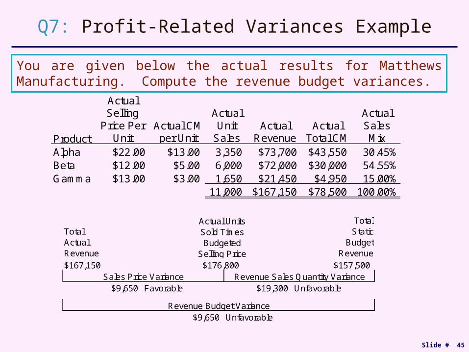
Q7: Profit-Related Variances Example
You are given below the actual results for Matthews Manufacturing. Compute the revenue budget variances.
Product
Actual Selling
Price Per Unit
Actual CM per Unit
Actual Unit
SalesActual
RevenueActual
Total CM
Actual Sales Mix
Alpha $22.00 $13.00 3,350 $73,700 $43,550 30.45%Beta $12.00 $5.00 6,000 $72,000 $30,000 54.55%Gamma $13.00 $3.00 1,650 $21,450 $4,950 15.00%
11,000 $167,150 $78,500 100.00%
Total Actual Revenue
Total Static
Budget Revenue
$9,650 Favorable $19,300 Unfavorable
Actual Units Sold Times Budgeted
Selling Price$176,800
Sales Price Variance Revenue Sales Quantity Variance$167,150 $157,500
Revenue Budget Variance$9,650 Unfavorable

Slide # 46
Q7: Profit-Related Variances Example
Use the given information on the prior two slides to compute all of the contribution margin budget variances for Matthews Manufacturing.
Total Static Budget CM
Actual Total Units Sold
Times Actual
Sales Mix Times
Actual CM $84,000 $78,500
$20,650
Actual Total Units Sold Times Actual Sales Mix Times Static Budget CM
per Unit$99,150
Favorable
Actual Total Units Sold Times Static Budget Sales Mix
Times Static Budget CM per Unit
CM Budget Variance$5,500 Unfavorable
CM Sales Volume Variance
$92,400CM Sales Quantity Variance
$8,400 Favorable $6,750
FavorableCM Variance
$15,150 Favorable
CM Sales Mix Variance

Slide # 47
JOIN KHALID AZIZ
• ECONOMICS OF ICMAP, ICAP, MA-ECONOMICS, B.COM.
• FINANCIAL ACCOUNTING OF ICMAP STAGE 1,3,4 ICAP MODULE B, B.COM, BBA, MBA & PIPFA.
• COST ACCOUNTING OF ICMAP STAGE 2,3 ICAP MODULE D, BBA, MBA & PIPFA.
• CONTACT:• 0322-3385752• R-1173,ALNOOR SOCIETY, BLOCK 19,F.B.AREA,
KARACHI, PAKISTAN.


![[KGIT_EWD]class03 0322](https://img.pdfslide.net/doc/110x75/555e0ca5d8b42a99188b4be1/kgitewdclass03-0322.jpg)