Slides for Chapter 12

Note to Instructors

License

© 2012 John S. Conery

The slides in this Keynote document are based on copyrighted material from Explorations in Computing: An Introduction to Computer Science, by John S. Conery.

These slides are provided free of charge to instructors who are using the textbook for their courses.

Instructors may alter the slides for use in their own courses, including but not limited to: adding new slides, altering the wording or images found on these slides, or deleting slides.

Instructors may distribute printed copies of the slides, either in hard copy or as electronic copies in PDF form, provided the copyright notice below is reproduced on the first slide.

This Keynote document contains the slides for “The Traveling Salesman”, Chapter 12 of Explorations in Computing: An Introduction to Computer Science.

The book invites students to explore ideas in computer science through interactive tutorials where they type expressions in Ruby and immediately see the results, either in a terminal window or a 2D graphics window.

Instructors are strongly encouraged to have a Ruby session running concurrently with Keynote in order to give live demonstrations of the Ruby code shown on the slides.

Explorations in Computing

© 2012 John S. Conery

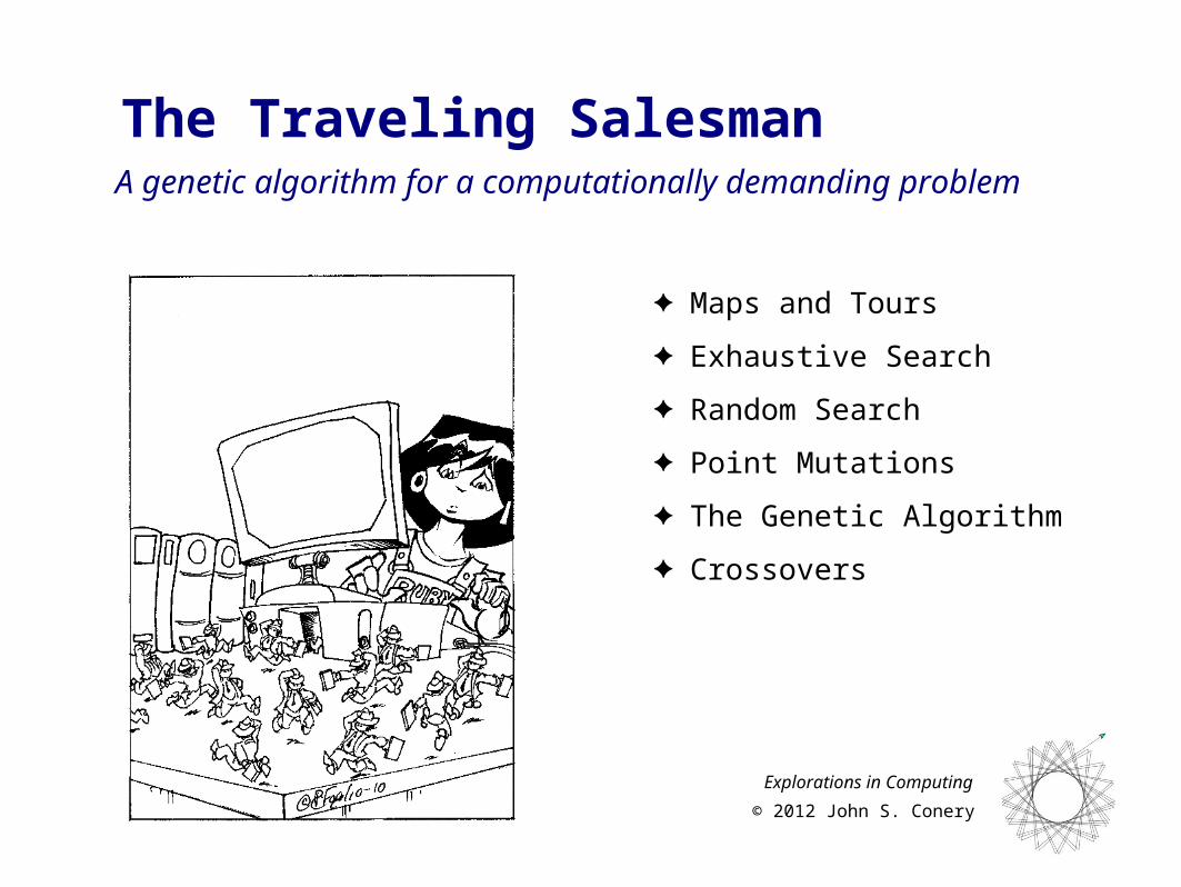
A genetic algorithm for a computationally demanding problem

The Traveling Salesman

✦ Maps and Tours

✦ Exhaustive Search

✦ Random Search

✦ Point Mutations

✦ The Genetic Algorithm

✦ Crossovers

Bike Tour

✦ Suppose you decide to ride a bicycle around Ireland❖ you will start in Dublin

❖ the goal is to visit Cork, Galway, Limerick, and Belfast before returning to Dublin

✦ What is the best itinerary?❖ how can you minimize the number of kilometers yet make sure you visit all the cities?

Optimal Tour

✦ If there are only 5 cities it’s not too hard to figure out the optimal tour❖ the shortest path is most likely a “loop”

❖ any path that crosses over itself will be longer than a path that travels in a big circle

Increasing the Number of Cities

✦ As we add cities to our tour, however, it is much harder to figure out the optimal tour❖ a simple strategy of going to the

closest city does not always lead to the shortest tour

❖ this example has 25 cities

❖ after visiting 4 cities, where would you go next?

Hint: going to this city does not lead to the shortest tour...

Exhaustive Search

✦ One way to find the optimal tour is to consider all possible paths

✦ The lab module for this chapter includes a class named Map that represents cities and distances between them

✦ If m is a Map object, this Ruby statement will consider all possible tours and save the one with the shortest distance:

>> m.each_tour { |t| best = t if t.cost < best.cost }

✦ The method named each_tour is just like the each method that iterates over a list❖it iterates over all possible tours

❖even though we don’t have an actual list of tours, this iteration is a type of search

❖computer scientists call it an exhaustive search since all combinations are tried

Too Many Tours

✦ There is a problem with the exhaustive search strategy❖ the number of possible tours of a map with n cities is (n − 1)! / 2

❖ n! (pronounced “n factorial”) is the product n × (n − 1) × (n − 2) ... × 2 × 1

✦ The number of tours grows incredibly quickly as we add cities to the map

#cities #tours

5 12

6 60

7 360

8 2,520

9 20,160

10 181,440The number of tours for 25 cities:

310,224,200,866,619,719,680,000

Real-Life Applications

✦ It’s not likely anyone would want to plan a bike trip to 25 cities

✦ But the solution of several important “real world” problems is the same as finding a tour of a large number of cities

❖ transportation: school bus routes, service calls, delivering meals, ...

❖ manufacturing: an industrial robot that drills holes in printed circuit boards

❖ VLSI (microchip) layout

❖ communication: planning newtelecommunication networks

For many of these problems n (the number of “cities”) can be

1,000 or more

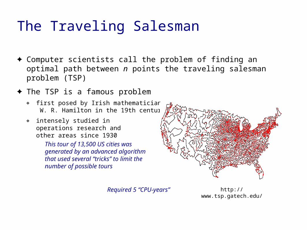
The Traveling Salesman

✦ Computer scientists call the problem of finding an optimal path between n points the traveling salesman problem (TSP)

✦ The TSP is a famous problem❖ first posed by Irish mathematician

W. R. Hamilton in the 19th century

❖ intensely studied in operations research and other areas since 1930

This tour of 13,500 US cities was generated by an advanced algorithm that used several “tricks” to limit the number of possible tours

http://www.tsp.gatech.edu/Required 5 “CPU-years”

Genetic Algorithm

✦ One way to approach the TSP is to use an evolutionary algorithm❖ the type of algorithm we will explore is known as a genetic algorithm

Imagine we have a Petri dish with several hundred different tours

In Ruby, each tour will be an separate object, each with a

different possible path

Evolutionary Algorithm (cont’d)

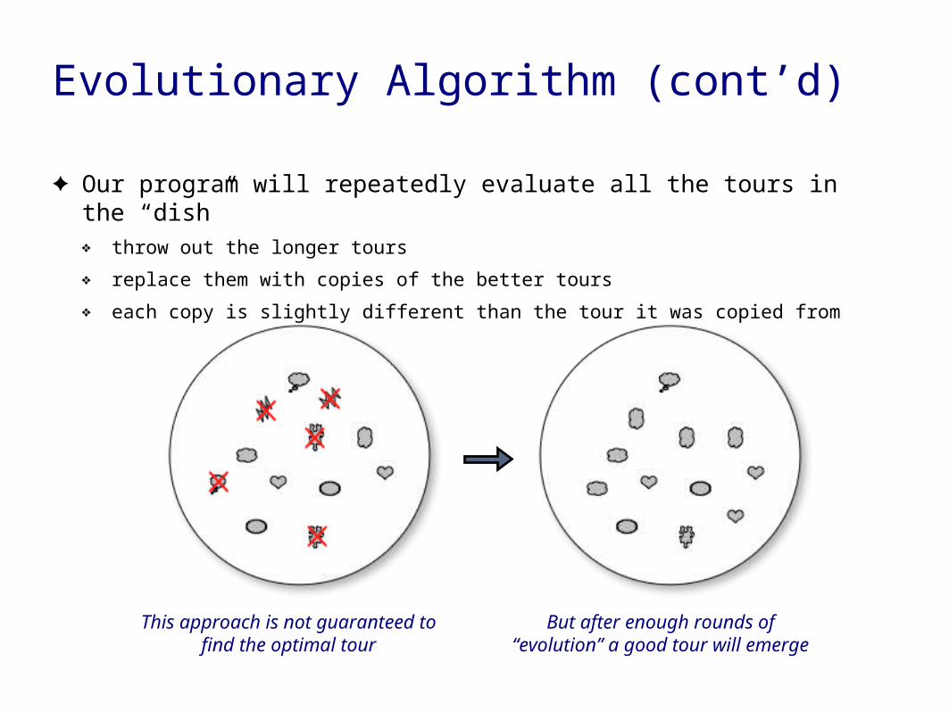
✦ Our program will repeatedly evaluate all the tours in the “dish”❖ throw out the longer tours

❖ replace them with copies of the better tours

❖ each copy is slightly different than the tour it was copied from

This approach is not guaranteed to find the optimal tour

But after enough rounds of “evolution” a good tour will emerge

TSPLab

✦ The lab module for this chapter is named TSPLab

✦ To explore the genetic algorithm we first need to create a map

✦ Pass a symbol to Map.new to create an object with predefined cities and distances:

>> m = Map.new(:ireland)

=> #<TSPLab::Map [belfast,cork,dublin,galway,limerick]>

✦ Or pass an integer to get a random map with a specified number of cities:

>> m = Map.new(10)

=> #<TSPLab::Map [0,1,2,3,4,5,6,7,8,9]>

Live Demo

Displaying a Map

✦ Call view_map to draw the cities on the RubyLabs canvas

Map of Ireland(5 cities)

10 cities, randomly placed

Distances Between Cities

✦ A Map object behaves like a matrix (also known as a 2D array)

✦ Use Ruby’s index operator to look up the distance between any two cities

✦ For example, if m is the map of Ireland:

>> m[:dublin, :galway]

=> 219.0

✦ If m is the map of random cities, the city names are just integers:

>> m[3,4]

=> 351.920445555526

>> m[0,7]

=> 213.356509157794City “names” in a random map are the

integers between 0 and n-1, e.g. 0 to 9 for a map of 10 cities

Tour Objects

✦ The Map class has a method named make_tour that will create a tour of all the cities

>> t = m.make_tour

=> #<TSPLab::Tour [0, 1, 2, 3, 4, 5, 6, 7, 8, 9] (1971.35)>

✦ Note the cities are in order

✦ To make a tour of the cities in some random order:

>> t = m.make_tour(:random)

=> #<TSPLab::Tour [6, 1, 9, 2, 8, 5, 4, 3, 0, 7] (2009.14)>

A random tour is a permutation of the list of cities.

See Ch. 9 for an algorithm that generates a random permutation of an array.

Displaying a Tour

✦ If the RubyLabs canvas is displaying a map, you can call view_tour to see the path for a tour

>> t.path

=> [6, 8, 7, 1, 0, 9, 5, 3, 4, 2]

>> view_tour(t)

=> true

Tour Cost

✦ In TSPLab the cost of a tour is the sum of the lengths of the paths between cities❖ in real applications, cost can be measured in several different ways, e.g. driving distance,

driving time, the cost of wires to connect circuits, etc

✦ If t is a Tour object, call t.cost to get the length of the tour:

>> t = m.make_tour([0,1,2])

=> #<TSPLab::Tour [0, 1, 2] (704.09)>

>> t.cost

=> 704.093753796085

>> m[0,1] + m[1,2] + m[2,0]

=> 704.093753796085

Make a short tour of only 3 cities on map m

Find the cost of this tour

The cost is computed by adding the length of each segment of the tour

An Experiment with Exhaustive Search

✦ If you want to see a list of all possible tours you can call each_tour

✦ For the map of Ireland:

>> m.each_tour { |t| p t.path }

[:belfast, :cork, :dublin, :galway, :limerick]

[:belfast, :cork, :dublin, :limerick, :galway]

[:belfast, :cork, :limerick, :dublin, :galway]

...

✦ But be careful: if you call each_tour for a map with 10 or more cities you might wait a while...

>> m.each_tour { |t| p t.path }

[0, 1, 2, 3, 4, 5, 6, 7, 8, 9]

[0, 1, 2, 3, 4, 5, 6, 7, 9, 8]

[0, 1, 2, 3, 4, 5, 6, 9, 7, 8]

...

This expression will print 12 tours

If you don’t want to wait for all 181,440 tours type ^C to interrupt Ruby

Counting Tours

✦ You can find out how many tours there are without calling each_tour and counting the number of lines it prints

✦ Call factorial to compute n! for some value of n:

>> factorial(10)

=> 3628800

✦ A method named ntours will compute (n−1)! / 2:

>> ntours(10)

=> 181440

See the text for an explanation of why there are (n−1)! / 2 tours on a map of n cities

Random Search

✦ One way to try to find an optimal tour is to take a “random sample”❖ simply generate lots of random tours and keep track of the best one

✦ We only need to enter two expressions in IRB

>> best = m.make_tour( :random )

>> 999.times { t = m.make_tour( :random ); best = t if t.cost < best.cost }

✦ Now the variable named best contains the lowest cost tour out of the 1000 random samples:

>> best

=> #<TSPLab::Tour [4, 5, 7, 2, 9, 8, 1, 3, 6, 0] (1353.70)>

The initial tour and the best of the 1000 random samples are displayed on the next slide

Initialize best with a random tour:

Make 999 more samples, update best when a sample has a lower cost:

Random Search Result

Initial sample, cost = 2134.26Best tour out of 1000 random samples,

cost = 1353.70

Random Search Experiments

✦ If you want to try some experiments with random tours you can use a method named rsearch

>> m = Map.new(25)

=> #<TSPLab::Map [0,1,2,3,4,5, ... 21,22,23,24]>

>> view_map(m)

=> true

>> rsearch(m, 1000)

=> #<TSPLab::Tour [12, 9, 4, 20, ... 21, 7, 10] (3914.55)>

Create a new Map object, this time with 25 cities:

Call view_map to display it on the RubyLabs canvas:

Call rsearch, passing it the map and the number of samples to make:

As the search progresses, the display will be updated to show the best tour found so far

Mutations

✦ The difference between random search and the genetic algorithm:

when we find a good tour, try to improve it

✦ Adopting terminology from molecular biology, changes to tours are called mutations

✦ A type of mutation that makes a minimal changein a cell is a point mutation

✦ In TSPLab, a point mutation exchangesthe order in which two cities are visited

Change a single base, e.g. A → C

... 16, 11, 7, 9, ...

... 16, 7, 11, 9, ...

Mutation Example

✦ A point mutation can improve a tour, as shown below❖ but not all mutations are beneficial

Path before mutation:... H, C, F, I, J, E, ...

Path after mutation:... H, C, I, F, J, E, ...

Mutations in TSPLab

✦ A method named mutate! will exchange two cities in a path❖ the argument passed to mutate! is an index i

❖ the method swaps path[i] and path[i+1]

✦ Here is an example, using a tour on a map of 25 cities:

>> t.path

=> [22, 0, 21, 1, 12, 18, 16, 15, ... 4, 6, 11]

>> t.mutate!(3)

>> t.path

=> [22, 0, 21, 12, 1, 18, 16, 15, ... 4, 6, 11]

The original path:

Recall the Ruby convention: methods that modify an object should have names that end with !

Check the new path:

Exchange path[3] and path[4]:

Evolutionary Search

✦ In order to implement the genetic algorithm mentioned earlier, we need to define the following:❖ a “virtual Petri dish” that will hold a collection of Tour objects

❖ a method that will iterate over the current tours and delete those with higher costs

❖ a method that will replace deleted tours with mutated copies of the survivors

✦ We’ll see how each of these operations are performed in TSPLab in the following slides

In the terminology of genetic algorithms, a collection of objects

is called a population

Initializing the Population

✦ Making a collection of random tours is simple❖ we just need to make an array and fill it with Tour objects, e.g.

>> p = []

>> 10.times { p << m.make_tour(:random) }

✦ In experiments with TSPLab, we can just call a method named init_population, passing it the map and the number of tours we want:

>> p = init_population(m, 10)

=> [ #<TSPLab::Tour [21, 4, 24, ... 0, 8] (4295.15)>, #<TSPLab::Tour [6, 8, 19, ... 11, 1] (4917.50>, ... #<TSPLab::Tour [23, 20, 24, ... 17, 7] (6035.68)> ]

Note: the tours are sorted according to cost, with lowest cost tours at the front of the array

Natural Selection

✦ Deleting tours is a process similar to natural selection in population biology❖ the most “fit” tours have lower costs

❖ in TSPLab, these tours are closest to the front of the population array

✦ A method named select_survivors iterates over the population❖ the tour at location i is deleted with probability i ÷ n, where n is the population size

✦ The table at right shows the probability of deleting an object from a population of 25 tours

i p(deletion)

0 0

1 0.04

2 0.08

... ...

23 0.92

24 0.96

The best tour is always kept

Note that poor tours may survive

Displaying Natural Selection

✦ If a map is being displayed on the RubyLabs canvas:❖ a call to init_population will display a bar graph

(example at right)

❖ the height of a bar represents the cost of a tour

❖ note the order, with low cost tours on the left

✦ Calling select_survivors will update the display❖ tours removed from the population will be colored gray

p = init_population(m, 10)

select_survivors(p)

Rebuilding the Population

✦ After the high cost tours are removed, the algorithm needs to refill the population❖ move all the survivors to the front of the array

❖ for each empty slot:

make a copy of a random survivor

add a point mutation to the copy

insert the copy into the array

✦ The operations are performed by a method named rebuild_population❖ the display will be updated

❖ new tours are on the right side of the histogram

esearch

✦ The operations described on the previous slides are all called by a method named esearch

✦ Two arguments must be passed in each call to esearch:❖ a Map object, which defines the cities and the distances between them

❖ the number of generations, i.e. the number of rounds of selection followed by rebuilding

✦ The method returns the best tour found after the specified number of generations

esearch(m, 500)

Population Size

✦ The effectiveness of the genetic algorithm implemented by esearch depends on several factors

✦ One is population size: with a larger population there is a better chance of creating a beneficial mutation❖ by default esearch makes a population of 10 tour objects

❖ pass an optional argument to specify a different population size, e.g.

>> esearch(m, 500, :popsize => 50)

✦ Try experimenting with different map sizes and population sizes❖ for small maps a population of 10 to 20 might work

❖ but for maps with 25 cities you will need populations of 50 or more

Note: the largest map you can make with RubyLabs is 400 cities

There is no predefined limit on the population size

Local Minima

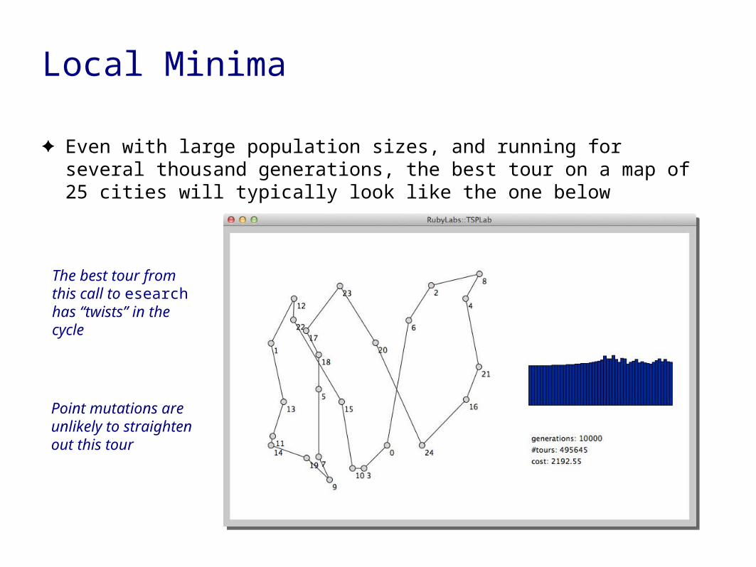
✦ Even with large population sizes, and running for several thousand generations, the best tour on a map of 25 cities will typically look like the one below

The best tour from this call to esearch has “twists” in the cycle

Point mutations are unlikely to straighten out this tour

Crossovers

✦ Another type of mutation inspired by the kinds of changes that occur in real cells can make more substantial changes to tours❖ in biology a crossover happens

when chromosomes from differentparents are split and recombine

❖ the new cell has partial strandsfrom both parents

✦ In TSPLab, a crossovermutation combines pathsfrom two different tours

Lodish, et al, Molecular Cell Biology (5th ed, 2004)

Crossover in TSPLab

✦ To perform a crossover, esearch selects two survivors❖ a random substring of the path is copied from one object

❖ the remaining cities are copied in order from the other object

The re-combined path can be better than either parent’s path

substring from parent 1’s path

substring from parent 2’s path

esearch with Crossovers

✦ To tell esearch to use a combination of point mutations and crossovers:

>> esearch(m, 500, :popsize => 100, :distribution => :mixed)

This map is the same as the one on a previous slide

A tour with no twists was found after a few hundred generations

Efficiency

✦ We can do some back-of-the-envelope calculations to estimate how many Tour objects are created by a call to esearch❖ on each generation roughly half the tours are replaced

❖ e.g. with popsize => 100 we expect to create 50 new Tour objects on each generation

✦ So the total number of Tour objects is approximately

n + g × (n / 2)

where n is the population size and g is the number of generations

✦ The search on the previous slide (n = 100, g = 500) examined only about 25,000 tour objects

Recap

✦ The traveling salesman problem is too complex to solve with a straightforward test of all possible paths❖ a map with 25 cities has over 3 × 1023 tours

✦ Instead of examining all possible tours, we can try taking a random sample❖ rsearch(m, n) will make n random tours, return the one with the lowest cost

✦ If we use ideas inspired by natural selection we can “evolve” the optimal tour by looking at far fewer samples❖ esearch(m, n) will simulate n generations

By looking at only 25,000 out of the 3 × 1023 possible tours esearch was able to find what might be the optimal tour.

Optimization

✦ The traveling salesman problem is an example of a more general type of problem known as optimization

✦ The goal is to find a combinationof parameters that give thehighest or lowest valuefor a function

graph for a function

z = f(x,y)

what values of x and y give the highest value of f?

Optimization Problems (cont’d)

✦ Another example: bin packing❖ the goal: choose a set of packages that will fill the most space on a truck

❖ a “greedy” algorithm puts the big boxes on first

❖ a better choice might include lots of smaller boxes

❖ an algorithm potentially has to examine all combinations

Finding the optimal set of boxes requires a genetic algorithm or some other type of “heuristic” search

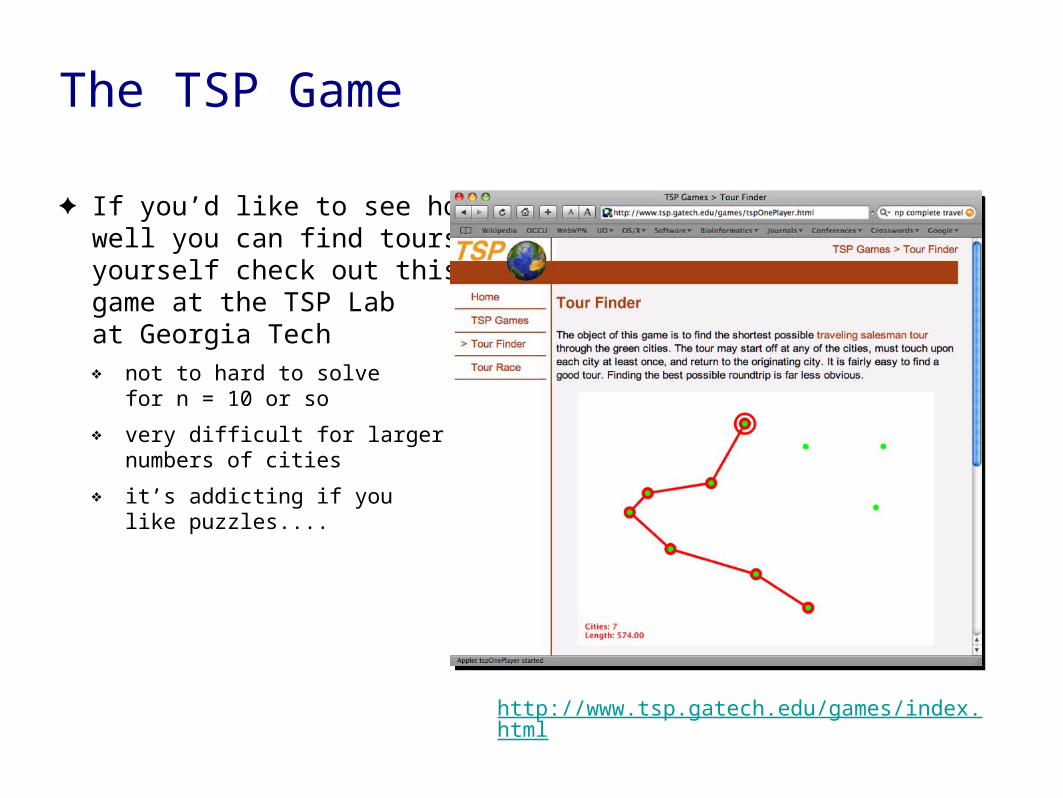
The TSP Game

✦ If you’d like to see howwell you can find toursyourself check out thisgame at the TSP Labat Georgia Tech❖ not to hard to solve

for n = 10 or so

❖ very difficult for largernumbers of cities

❖ it’s addicting if youlike puzzles....

http://www.tsp.gatech.edu/games/index.html