Embed Size (px)
Citation preview
11SlideSlide©© 2006 Thomson/South2006 Thomson/South--WesternWestern
Slides Prepared by
JOHN S. LOUCKSSt. Edward’s University
Slides Prepared bySlides Prepared by
JOHN S. LOUCKSJOHN S. LOUCKSSt. EdwardSt. Edward’’s Universitys University

22SlideSlide©© 2006 Thomson/South2006 Thomson/South--WesternWestern
Chapter 13Chapter 13Multiple RegressionMultiple Regression
Multiple Regression ModelMultiple Regression ModelLeast Squares MethodLeast Squares MethodMultiple Coefficient of DeterminationMultiple Coefficient of DeterminationModel AssumptionsModel AssumptionsTesting for SignificanceTesting for SignificanceUsing the Estimated Regression EquationUsing the Estimated Regression Equation
for Estimation and Predictionfor Estimation and PredictionQualitative Independent VariablesQualitative Independent Variables
33SlideSlide©© 2006 Thomson/South2006 Thomson/South--WesternWestern
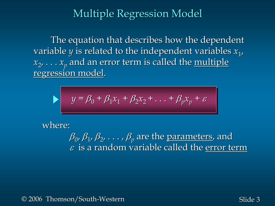
The equation that describes how the dependent The equation that describes how the dependent variable variable yy is related to the independent variables is related to the independent variables xx11, , xx22, . . . , . . . xxpp and an error term is called the and an error term is called the multiplemultipleregression modelregression model..
Multiple Regression ModelMultiple Regression Model
yy = = ββ00 + + ββ11xx11 + + ββ22xx2 2 ++ . . . +. . . + ββppxxpp + + εε
where:where:ββ00, , ββ11, , ββ22, . . . ,, . . . , ββpp are the are the parametersparameters, and, andεε is a random variable called the is a random variable called the error termerror term
44SlideSlide©© 2006 Thomson/South2006 Thomson/South--WesternWestern
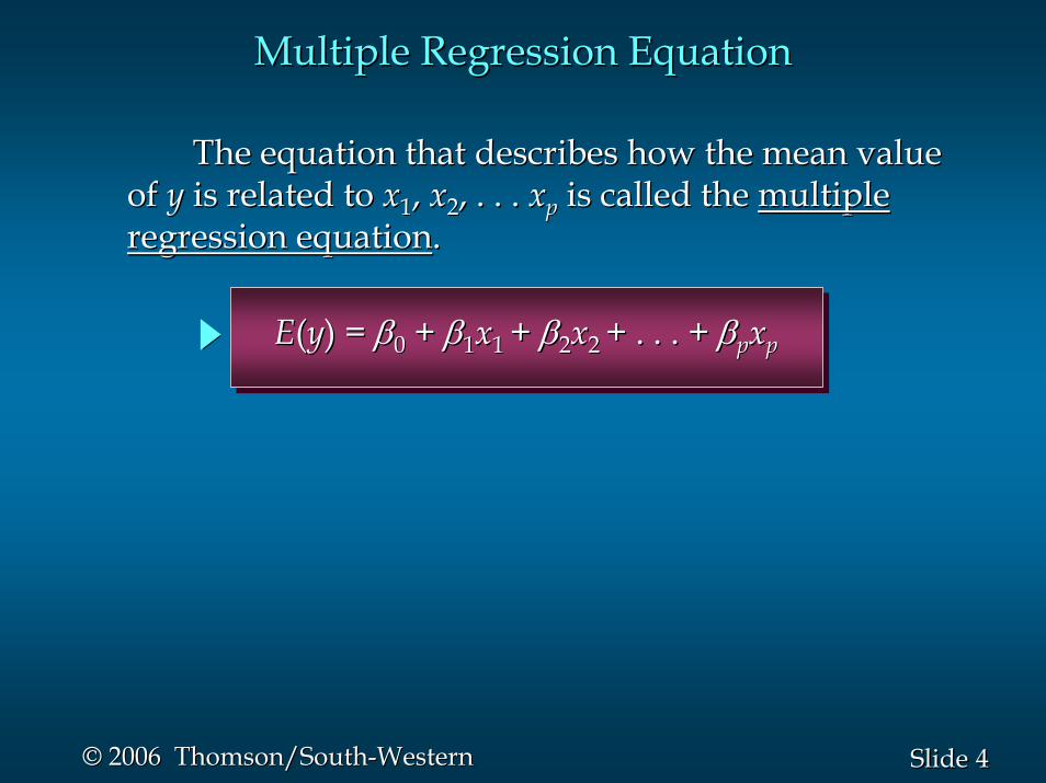
The equation that describes how the mean value The equation that describes how the mean value of of yy is related to is related to xx11, , xx22, . . ., . . . xxpp is called the is called the multiple multiple regression equationregression equation..
EE((yy) = ) = ββ00 + + ββ11xx1 1 + + ββ22xx2 2 + . . . + + . . . + ββppxxpp
Multiple Regression EquationMultiple Regression Equation
55SlideSlide©© 2006 Thomson/South2006 Thomson/South--WesternWestern
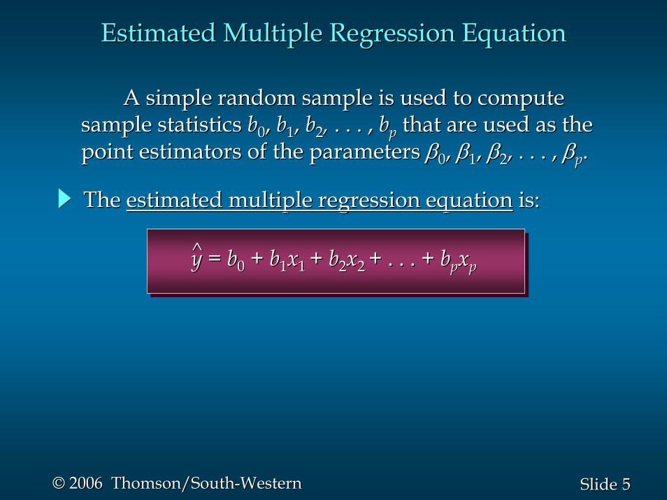
A simple random sample is used to compute A simple random sample is used to compute sample statistics sample statistics bb00, , bb11, , bb22, , . . . , . . . , bbpp that are used as the that are used as the point estimators of the parameters point estimators of the parameters ββ00, , ββ11, , ββ22, . . . , , . . . , ββpp..
Estimated Multiple Regression EquationEstimated Multiple Regression Equation
^̂yy = = bb00 + + bb11xx1 1 + + bb22xx2 2 + . . . ++ . . . + bbppxxpp
The The estimated multiple regression equationestimated multiple regression equation is:is:
66SlideSlide©© 2006 Thomson/South2006 Thomson/South--WesternWestern
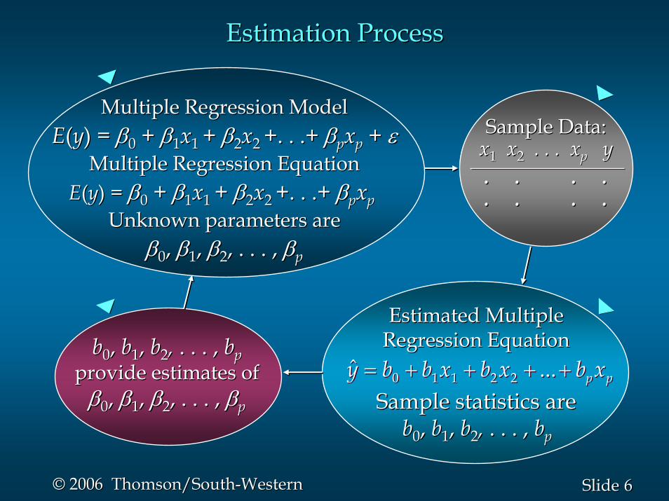
Estimation ProcessEstimation Process
Multiple Regression ModelMultiple Regression ModelEE((yy) = ) = ββ00 + + ββ11xx1 1 + + ββ22xx2 2 +. . .+ +. . .+ ββppxxpp + + εε
Multiple Regression EquationMultiple Regression EquationEE((yy) = ) = ββ00 + + ββ11xx1 1 + + ββ22xx2 2 +. . .+ +. . .+ ββppxxpp
Unknown parameters areUnknown parameters areββ00, , ββ11, , ββ22, . . . , , . . . , ββpp
Sample Data:Sample Data:xx11 xx22 . . .. . . xxpp yy. . . .. . . .. . . .. . . .
0 1 1 2 2ˆ ... p py b b x b x b x= + + + +0 1 1 2 2ˆ ... p py b b x b x b x= + + + +
Estimated MultipleEstimated MultipleRegression EquationRegression Equation
Sample statistics areSample statistics arebb00, , bb11, , bb22, , . . . , . . . , bbp p
bb00, , bb11, , bb22, , . . . ,. . . , bbppprovide estimates ofprovide estimates of
ββ00, , ββ11, , ββ22, . . . ,, . . . , ββpp
77SlideSlide©© 2006 Thomson/South2006 Thomson/South--WesternWestern
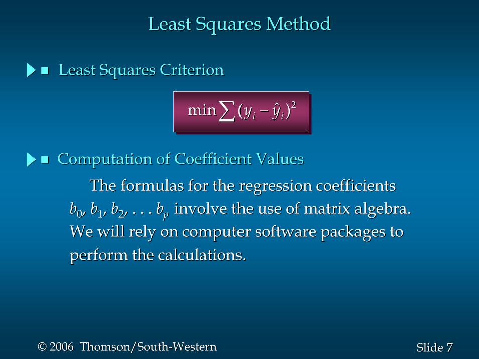
Least Squares MethodLeast Squares Method
Least Squares CriterionLeast Squares Criterion
2ˆmin ( )i iy y−∑ 2ˆmin ( )i iy y−∑
Computation of Coefficient ValuesComputation of Coefficient Values
The formulas for the regression coefficientsThe formulas for the regression coefficientsbb00, , bb11, , bb22, . . ., . . . bbp p involve the use of matrix algebra. involve the use of matrix algebra. We will rely on computer software packages toWe will rely on computer software packages toperform the calculations.perform the calculations.
88SlideSlide©© 2006 Thomson/South2006 Thomson/South--WesternWestern
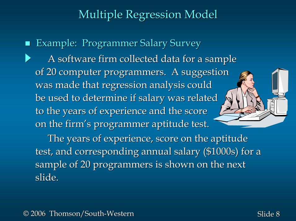
The years of experience, score on the aptitudeThe years of experience, score on the aptitudetest, and corresponding annual salary ($1000s) for a test, and corresponding annual salary ($1000s) for a sample of 20 programmers is shown on the nextsample of 20 programmers is shown on the nextslide.slide.
Example: Programmer Salary SurveyExample: Programmer Salary Survey
Multiple Regression ModelMultiple Regression Model
A software firm collected data for a sampleA software firm collected data for a sampleof 20 computer programmers. A suggestionof 20 computer programmers. A suggestionwas made that regression analysis couldwas made that regression analysis couldbe used to determine if salary was relatedbe used to determine if salary was relatedto the years of experience and the scoreto the years of experience and the scoreon the firmon the firm’’s programmer aptitude test.s programmer aptitude test.
99SlideSlide©© 2006 Thomson/South2006 Thomson/South--WesternWestern
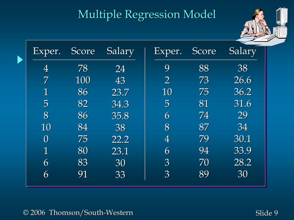
4477115588101000116666
9922101055668844663333
787810010086868282868684847575808083839191
8888737375758181747487877979949470708989
24244343
23.723.734.334.335.835.83838
22.222.223.123.130303333
383826.626.636.236.231.631.629293434
30.130.133.933.928.228.23030
ExperExper.. ScoreScore ScoreScoreExperExper..SalarySalary SalarySalary
Multiple Regression ModelMultiple Regression Model
1010SlideSlide©© 2006 Thomson/South2006 Thomson/South--WesternWestern
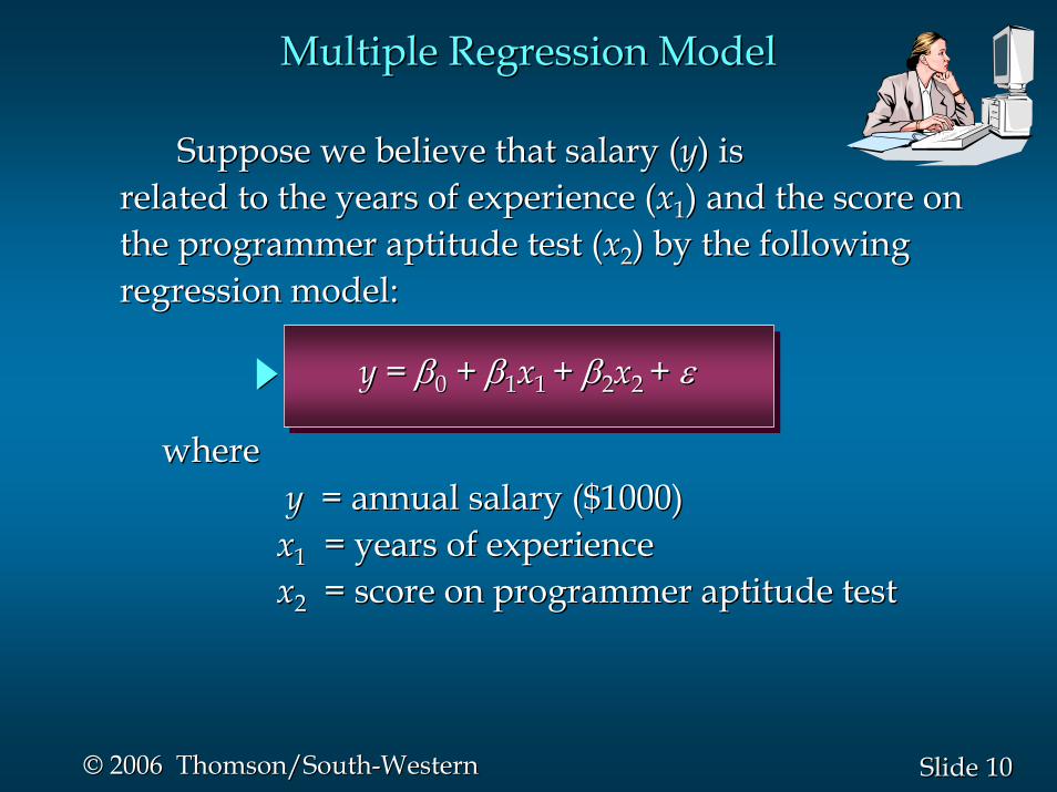
Suppose we believe that salary (Suppose we believe that salary (yy) is) isrelated to the years of experience (related to the years of experience (xx11) and the score on) and the score onthe programmer aptitude test (the programmer aptitude test (xx22) by the following ) by the following regression model:regression model:
Multiple Regression ModelMultiple Regression Model
wherewhereyy = annual salary ($1000)= annual salary ($1000)xx11 = years of experience= years of experiencexx22 = score on programmer aptitude test= score on programmer aptitude test
yy = = ββ00 + + ββ11xx1 1 + + ββ22xx2 2 + + εε

1111SlideSlide©© 2006 Thomson/South2006 Thomson/South--WesternWestern
Solving for the Estimates of Solving for the Estimates of ββ00, , ββ11, , ββ22
Input DataInput DataLeast SquaresLeast Squares
OutputOutput
xx11 xx22 yy
4 78 244 78 247 100 437 100 43. . .. . .. . .. . .3 89 303 89 30
ComputerComputerPackagePackage
for Solvingfor SolvingMultipleMultiple
RegressionRegressionProblemsProblems
bb00 = = bb11 ==bb22 ==
RR22 ==
etc.etc.
1212SlideSlide©© 2006 Thomson/South2006 Thomson/South--WesternWestern
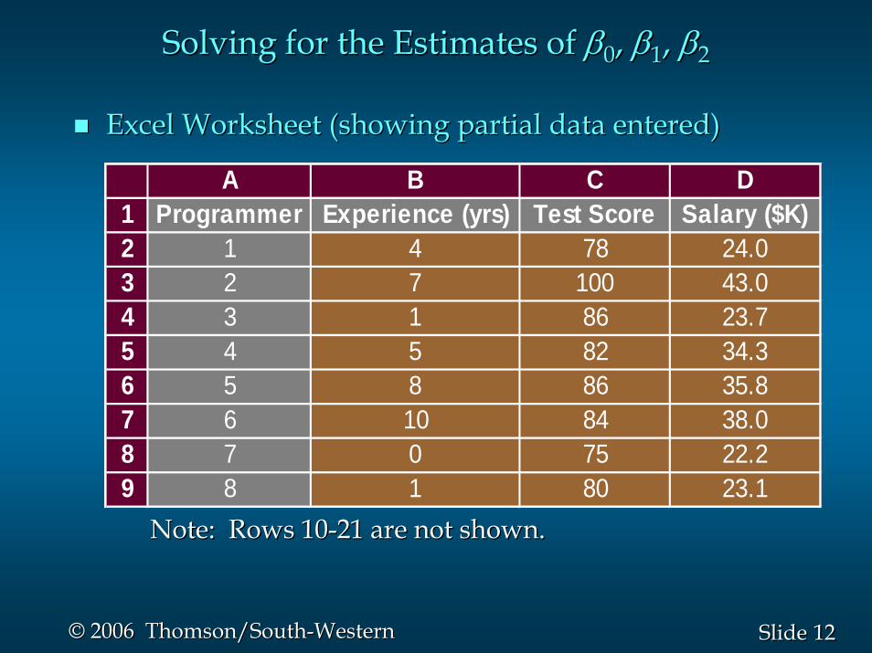
Excel Worksheet (showing partial data entered)Excel Worksheet (showing partial data entered)
A B C D1 Programmer Experience (yrs) Test Score Salary ($K)2 1 4 78 24.03 2 7 100 43.04 3 1 86 23.75 4 5 82 34.36 5 8 86 35.87 6 10 84 38.08 7 0 75 22.29 8 1 80 23.1
Note: Rows 10Note: Rows 10--21 are not shown.21 are not shown.
Solving for the Estimates of Solving for the Estimates of ββ00, , ββ11, , ββ22
1313SlideSlide©© 2006 Thomson/South2006 Thomson/South--WesternWestern
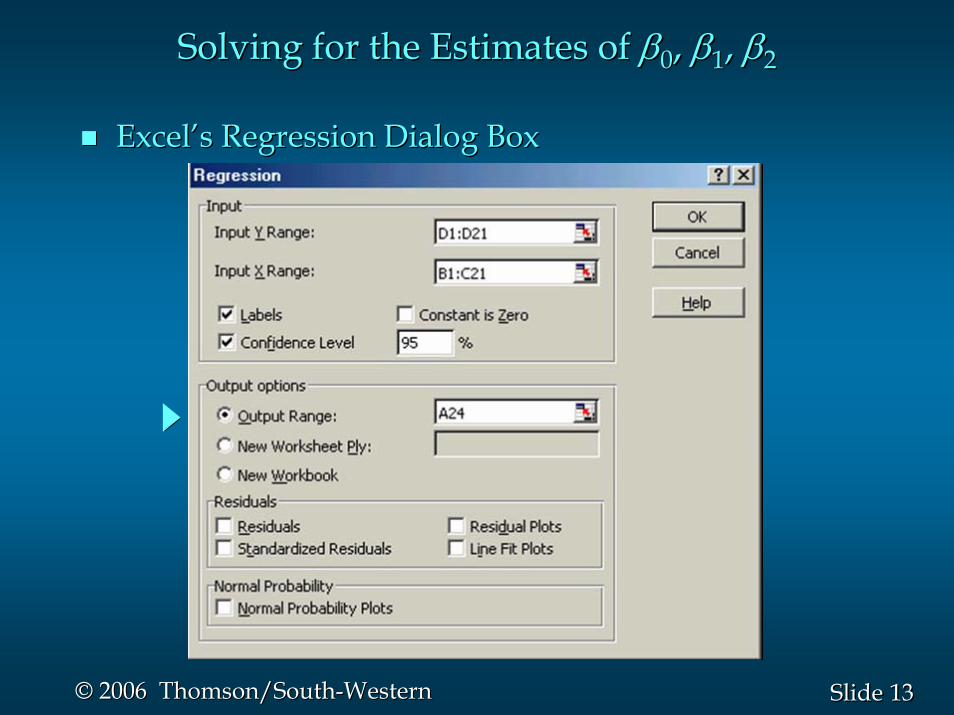
ExcelExcel’’s Regression Dialog Boxs Regression Dialog Box
Solving for the Estimates of Solving for the Estimates of ββ00, , ββ11, , ββ22
1414SlideSlide©© 2006 Thomson/South2006 Thomson/South--WesternWestern
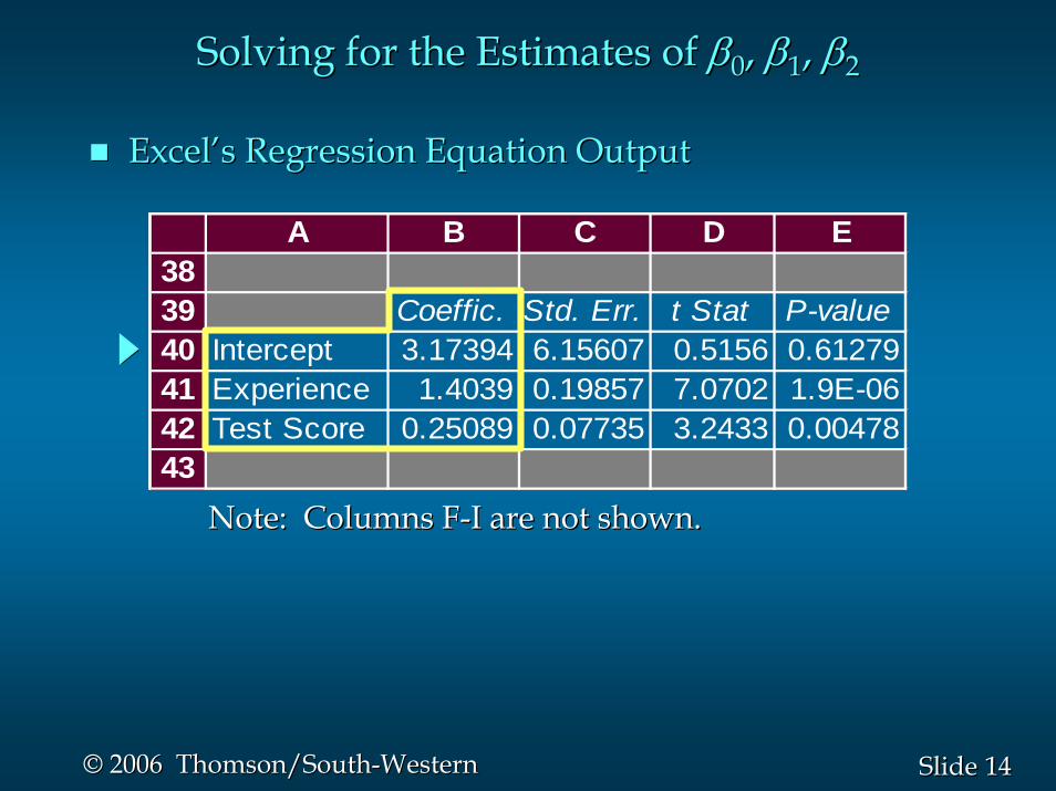
ExcelExcel’’s Regression Equation Outputs Regression Equation Output
A B C D E3839 Coeffic. Std. Err. t Stat P-value40 Intercept 3.17394 6.15607 0.5156 0.6127941 Experience 1.4039 0.19857 7.0702 1.9E-0642 Test Score 0.25089 0.07735 3.2433 0.0047843
Note: Columns FNote: Columns F--I are not shown.I are not shown.
Solving for the Estimates of Solving for the Estimates of ββ00, , ββ11, , ββ22
1515SlideSlide©© 2006 Thomson/South2006 Thomson/South--WesternWestern
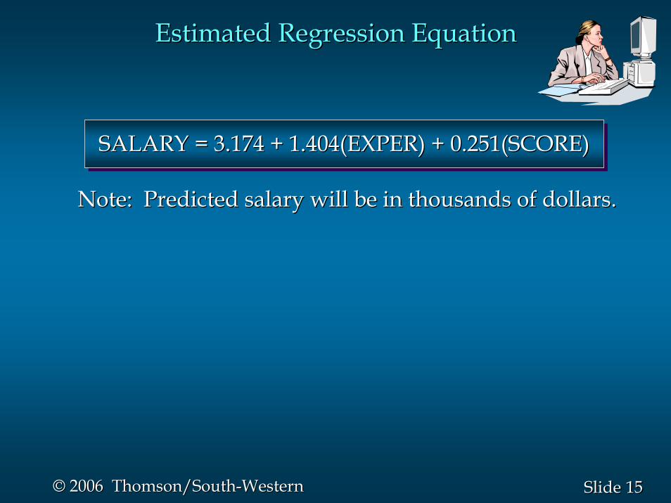
Estimated Regression EquationEstimated Regression Equation
SALARY = 3.174 + 1.404(EXPER) + 0.251(SCORE)SALARY = 3.174 + 1.404(EXPER) + 0.251(SCORE)SALARY = 3.174 + 1.404(EXPER) + 0.251(SCORE)
Note: Predicted salary will be in thousands of dollars.Note: Predicted salary will be in thousands of dollars.

1616SlideSlide©© 2006 Thomson/South2006 Thomson/South--WesternWestern
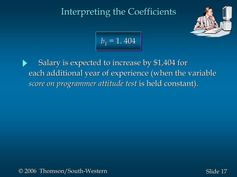
Interpreting the CoefficientsInterpreting the Coefficients
In multiple regression analysis, we interpret eachIn multiple regression analysis, we interpret eachregression coefficient as follows:regression coefficient as follows:
bbii represents an estimate of the change in represents an estimate of the change in yycorresponding to a 1corresponding to a 1--unit increase in unit increase in xxii when allwhen allother independent variables are held constant.other independent variables are held constant.
1717SlideSlide©© 2006 Thomson/South2006 Thomson/South--WesternWestern
Salary is expected to increase by $1,404 for Salary is expected to increase by $1,404 for each additional year of experience (when the variableeach additional year of experience (when the variablescore on programmer attitude testscore on programmer attitude test is held constant).is held constant).
b1 = 1. 404bb11 = 1. 404= 1. 404
Interpreting the CoefficientsInterpreting the Coefficients

1818SlideSlide©© 2006 Thomson/South2006 Thomson/South--WesternWestern
Salary is expected to increase by $251 for eachSalary is expected to increase by $251 for eachadditional point scored on the programmer aptitudeadditional point scored on the programmer aptitude
test (when the variable test (when the variable years of experienceyears of experience is heldis heldconstant).constant).
b2 = 0.251bb22 = 0.251= 0.251
Interpreting the CoefficientsInterpreting the Coefficients

1919SlideSlide©© 2006 Thomson/South2006 Thomson/South--WesternWestern
Multiple Coefficient of DeterminationMultiple Coefficient of Determination
Relationship Among SST, SSR, SSERelationship Among SST, SSR, SSE
where:where:SST = total sum of squaresSST = total sum of squaresSSR = sum of squares due to regressionSSR = sum of squares due to regressionSSE = sum of squares due to errorSSE = sum of squares due to error
SST = SST = SSR SSR + + SSESSE
2( )iy y−∑ 2( )iy y−∑ 2ˆ( )iy y= −∑ 2ˆ( )iy y= −∑ 2ˆ( )i iy y+ −∑ 2ˆ( )i iy y+ −∑
2020SlideSlide©© 2006 Thomson/South2006 Thomson/South--WesternWestern
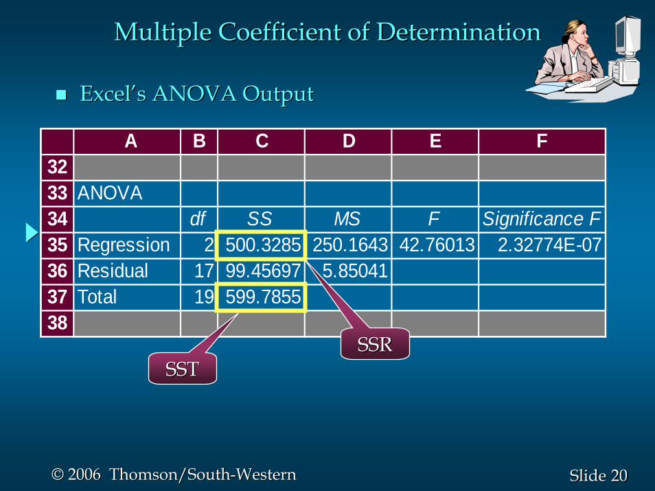
ExcelExcel’’s ANOVA Outputs ANOVA Output
A B C D E F3233 ANOVA34 df SS MS F Significance F35 Regression 2 500.3285 250.1643 42.76013 2.32774E-0736 Residual 17 99.45697 5.8504137 Total 19 599.785538
SSTSSTSSRSSR
Multiple Coefficient of DeterminationMultiple Coefficient of Determination
2121SlideSlide©© 2006 Thomson/South2006 Thomson/South--WesternWestern
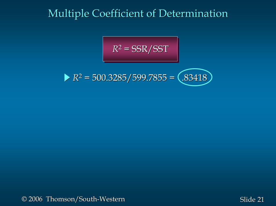
Multiple Coefficient of DeterminationMultiple Coefficient of Determination
RR22 = 500.3285/599.7855 = = 500.3285/599.7855 = .83418.83418
RR22 = SSR/SST= SSR/SST
2222SlideSlide©© 2006 Thomson/South2006 Thomson/South--WesternWestern
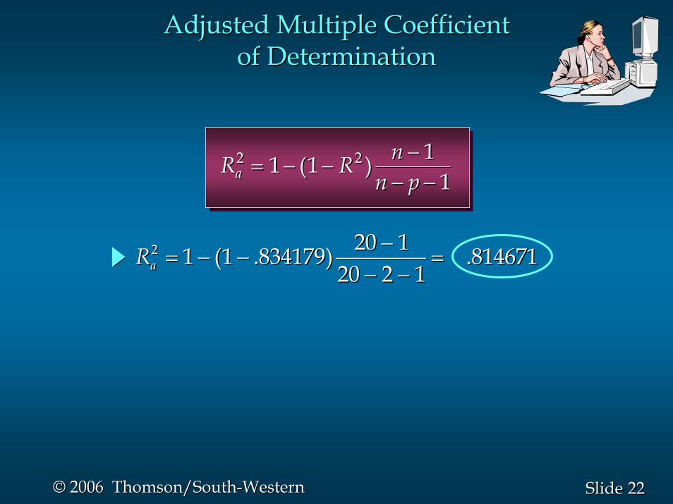
Adjusted Multiple CoefficientAdjusted Multiple Coefficientof Determinationof Determination
R R nn pa
2 21 1 11
= − −−
− −( )R R n
n pa2 21 1 1
1= − −
−− −
( )
2 20 11 (1 .834179) .81467120 2 1aR −
= − − =− −
2 20 11 (1 .834179) .81467120 2 1aR −
= − − =− −

2323SlideSlide©© 2006 Thomson/South2006 Thomson/South--WesternWestern
ExcelExcel’’s Regression Statisticss Regression Statistics
A B C23 24 SUMMARY OUTPUT2526 Regression Statistics27 Multiple R 0.91333405928 R Square 0.83417910329 Adjusted R Square 0.81467076230 Standard Error 2.41876207631 Observations 2032
Adjusted Multiple CoefficientAdjusted Multiple Coefficientof Determinationof Determination
2424SlideSlide©© 2006 Thomson/South2006 Thomson/South--WesternWestern
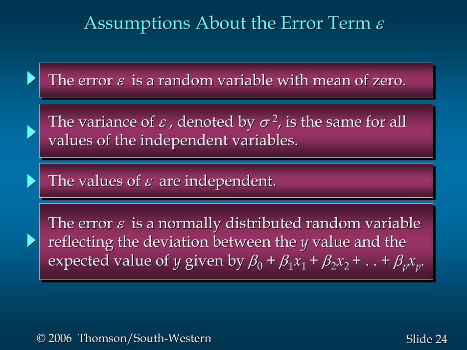
The variance of ε , denoted by σ 2, is the same for allvalues of the independent variables.The variance of The variance of εε , denoted by , denoted by σ σ 22, is the same for all, is the same for allvalues of the independent variables.values of the independent variables.
The error ε is a normally distributed random variablereflecting the deviation between the y value and theexpected value of y given by β0 + β1x1 + β2x2 + . . + βpxp.
The error The error εε is a normally distributed random variableis a normally distributed random variablereflecting the deviation between the reflecting the deviation between the yy value and thevalue and theexpected value of expected value of yy given by given by ββ00 + + ββ11xx1 1 + + ββ22xx2 2 + . . + + . . + ββppxxpp..
Assumptions About the Error Term Assumptions About the Error Term εε
The error ε is a random variable with mean of zero.The error The error εε is a random variable with mean of zero.is a random variable with mean of zero.
The values of ε are independent.The values of The values of εε are independent.are independent.
2525SlideSlide©© 2006 Thomson/South2006 Thomson/South--WesternWestern
In simple linear regression, the F and t tests providethe same conclusion.In simple linear regression, the In simple linear regression, the FF and and tt tests providetests providethe same conclusion.the same conclusion.
Testing for SignificanceTesting for Significance
In multiple regression, the F and t tests have differentpurposes.In multiple regression, the In multiple regression, the FF and and tt tests have differenttests have differentpurposes.purposes.
2626SlideSlide©© 2006 Thomson/South2006 Thomson/South--WesternWestern
Testing for Significance: Testing for Significance: F F TestTest
The F test is referred to as the test for overallsignificance.The The FF test is referred to as the test is referred to as the test for overalltest for overallsignificancesignificance..
The F test is used to determine whether a significantrelationship exists between the dependent variableand the set of all the independent variables.
The The FF test is used to determine whether a significanttest is used to determine whether a significantrelationship exists between the dependent variablerelationship exists between the dependent variableand the set of and the set of all the independent variablesall the independent variables..
2727SlideSlide©© 2006 Thomson/South2006 Thomson/South--WesternWestern
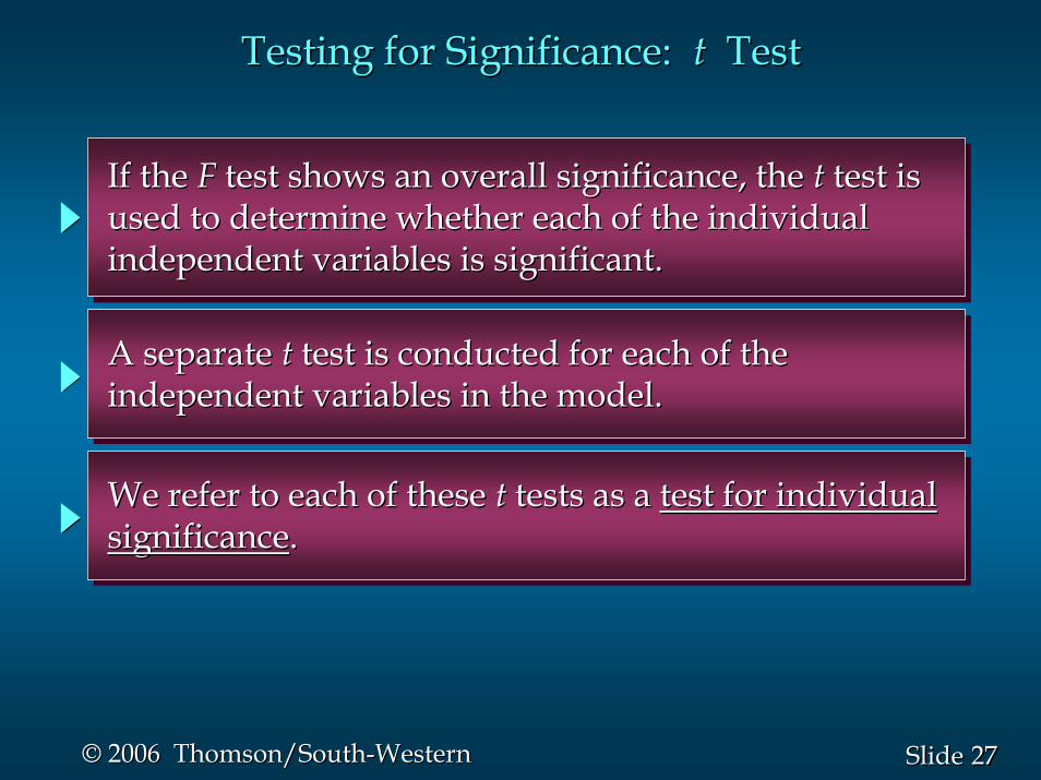
A separate t test is conducted for each of theindependent variables in the model.A separate A separate tt test is conducted for each of thetest is conducted for each of theindependent variables in the model.independent variables in the model.
If the F test shows an overall significance, the t test isused to determine whether each of the individualindependent variables is significant.
If the If the FF test shows an overall significance, the test shows an overall significance, the tt test istest isused to determine whether each of the individualused to determine whether each of the individualindependent variables is significant.independent variables is significant.
Testing for Significance: Testing for Significance: t t TestTest
We refer to each of these t tests as a test for individualsignificance.We refer to each of these We refer to each of these tt tests as a tests as a test for individualtest for individualsignificancesignificance..
2828SlideSlide©© 2006 Thomson/South2006 Thomson/South--WesternWestern
Testing for Significance: Testing for Significance: F F TestTest
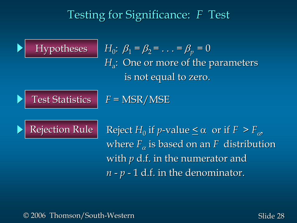
HypothesesHypotheses
Rejection RuleRejection Rule
Test StatisticsTest Statistics FF = MSR/MSE= MSR/MSE
HH00: : ββ11 = = ββ2 2 = . . . = = . . . = ββp p = 0= 0HHaa: One or more of the parameters: One or more of the parameters
is not equal to zero.is not equal to zero.
Reject Reject HH00 if if pp--value value << αα or if or if FF > > FFαα,,where where FFαα is based on an is based on an FF distributiondistributionwith with pp d.f. in the numerator andd.f. in the numerator andnn -- pp -- 1 d.f. in the denominator.1 d.f. in the denominator.

2929SlideSlide©© 2006 Thomson/South2006 Thomson/South--WesternWestern
F F Test for Overall SignificanceTest for Overall Significance
HypothesesHypotheses HH00: : ββ11 = = ββ2 2 = 0= 0HHaa: One or both of the parameters: One or both of the parameters
is not equal to zero.is not equal to zero.
Rejection RuleRejection Rule For For αα = .05 and d.f. = 2, 17; = .05 and d.f. = 2, 17; FF.05.05 = 3.59= 3.59Reject Reject HH00 if if pp--value value << .05 or .05 or FF >> 3.593.59
3030SlideSlide©© 2006 Thomson/South2006 Thomson/South--WesternWestern
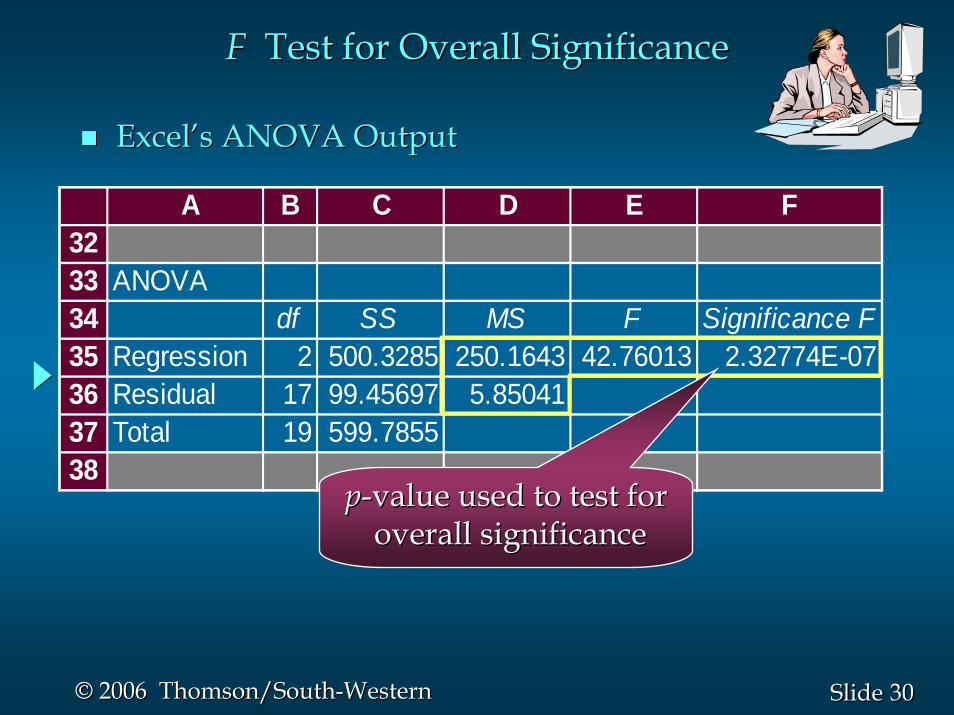
ExcelExcel’’s ANOVA Outputs ANOVA Output
A B C D E F3233 ANOVA34 df SS MS F Significance F35 Regression 2 500.3285 250.1643 42.76013 2.32774E-0736 Residual 17 99.45697 5.8504137 Total 19 599.785538
F F Test for Overall SignificanceTest for Overall Significance
pp--value used to test forvalue used to test foroverall significanceoverall significance
3131SlideSlide©© 2006 Thomson/South2006 Thomson/South--WesternWestern
F F Test for Overall SignificanceTest for Overall Significance
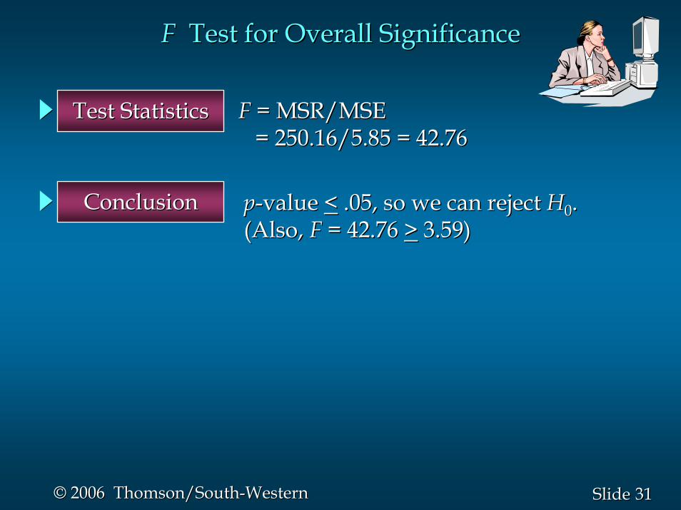
Test StatisticsTest Statistics FF = MSR/MSE= MSR/MSE= 250.16/5.85 = 42.76= 250.16/5.85 = 42.76
ConclusionConclusion pp--value value << .05, so we can reject .05, so we can reject HH00..(Also, (Also, FF = 42.76 = 42.76 >> 3.59)3.59)
3232SlideSlide©© 2006 Thomson/South2006 Thomson/South--WesternWestern
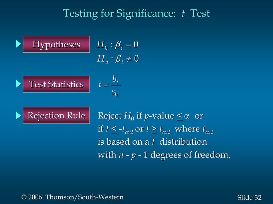
Testing for Significance: Testing for Significance: t t TestTest
HypothesesHypotheses
Rejection RuleRejection Rule
Test StatisticsTest Statistics
Reject Reject HH00 if if pp--value value << αα ororif if tt << --ttα/α/2 2 or or tt >> ttα/α/2 2 where where ttα/α/22
is based on a is based on a t t distributiondistributionwith with nn -- pp -- 1 degrees of freedom.1 degrees of freedom.
t bs
i
bi
=t bs
i
bi
=
0 : 0iH β =0 : 0iH β =
: 0a iH β ≠: 0a iH β ≠
3333SlideSlide©© 2006 Thomson/South2006 Thomson/South--WesternWestern
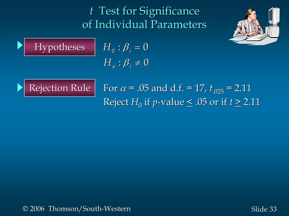
tt Test for SignificanceTest for Significanceof Individual Parametersof Individual Parameters
HypothesesHypotheses
Rejection RuleRejection Rule For For αα = .05 and d.f. = 17, = .05 and d.f. = 17, tt.025.025 = 2.11= 2.11Reject Reject HH00 if if pp--value value << .05 or if .05 or if tt >> 2.112.11
0 : 0iH β =0 : 0iH β =
: 0a iH β ≠: 0a iH β ≠
3434SlideSlide©© 2006 Thomson/South2006 Thomson/South--WesternWestern
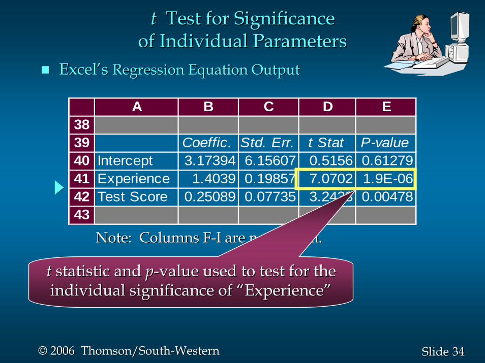
ExcelExcel’’s s Regression Equation OutputRegression Equation Output
A B C D E3839 Coeffic. Std. Err. t Stat P-value40 Intercept 3.17394 6.15607 0.5156 0.6127941 Experience 1.4039 0.19857 7.0702 1.9E-0642 Test Score 0.25089 0.07735 3.2433 0.0047843
Note: Columns FNote: Columns F--I are not shown.I are not shown.
tt Test for SignificanceTest for Significanceof Individual Parametersof Individual Parameters
tt statistic and statistic and pp--value used to test for the value used to test for the individual significance of individual significance of ““ExperienceExperience””
3535SlideSlide©© 2006 Thomson/South2006 Thomson/South--WesternWestern
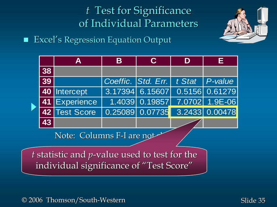
ExcelExcel’’s s Regression Equation OutputRegression Equation Output
A B C D E3839 Coeffic. Std. Err. t Stat P-value40 Intercept 3.17394 6.15607 0.5156 0.6127941 Experience 1.4039 0.19857 7.0702 1.9E-0642 Test Score 0.25089 0.07735 3.2433 0.0047843
Note: Columns FNote: Columns F--I are not shown.I are not shown.
tt Test for SignificanceTest for Significanceof Individual Parametersof Individual Parameters
tt statistic and statistic and pp--value used to test for the value used to test for the individual significance of individual significance of ““Test ScoreTest Score””
3636SlideSlide©© 2006 Thomson/South2006 Thomson/South--WesternWestern
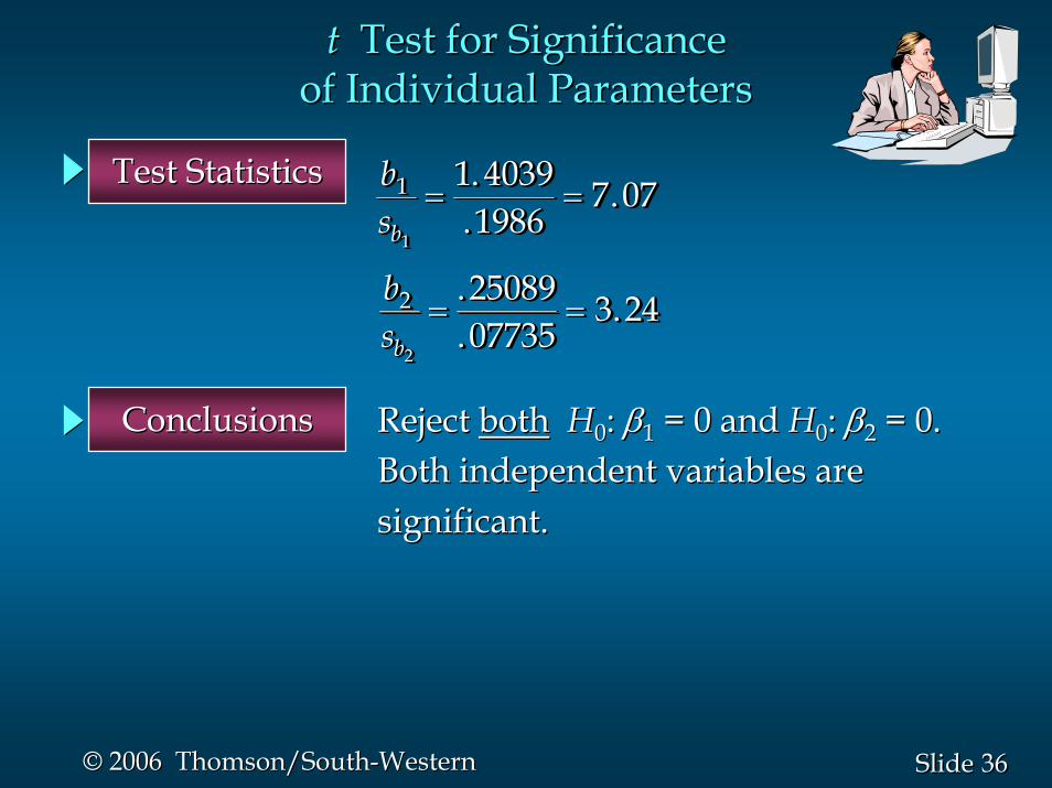
tt Test for SignificanceTest for Significanceof Individual Parametersof Individual Parameters
bsb
1
1
1 40391986
7 07= =..
.bsb
1
1
1 40391986
7 07= =..
.bsb
1
1
1 40391986
7 07= =..
.bsb
1
1
1 40391986
7 07= =..
.
bsb
2
2
2508907735
3 24= =..
.bsb
2
2
2508907735
3 24= =..
.bsb
2
2
2508907735
3 24= =..
.bsb
2
2
2508907735
3 24= =..
.
Test StatisticsTest Statistics
ConclusionsConclusions Reject Reject bothboth HH00: : ββ11 = 0 and = 0 and HH00: : ββ22 = 0.= 0.Both independent variables areBoth independent variables aresignificant.significant.
3737SlideSlide©© 2006 Thomson/South2006 Thomson/South--WesternWestern
Testing for Significance:Testing for Significance: Multicollinearity Multicollinearity
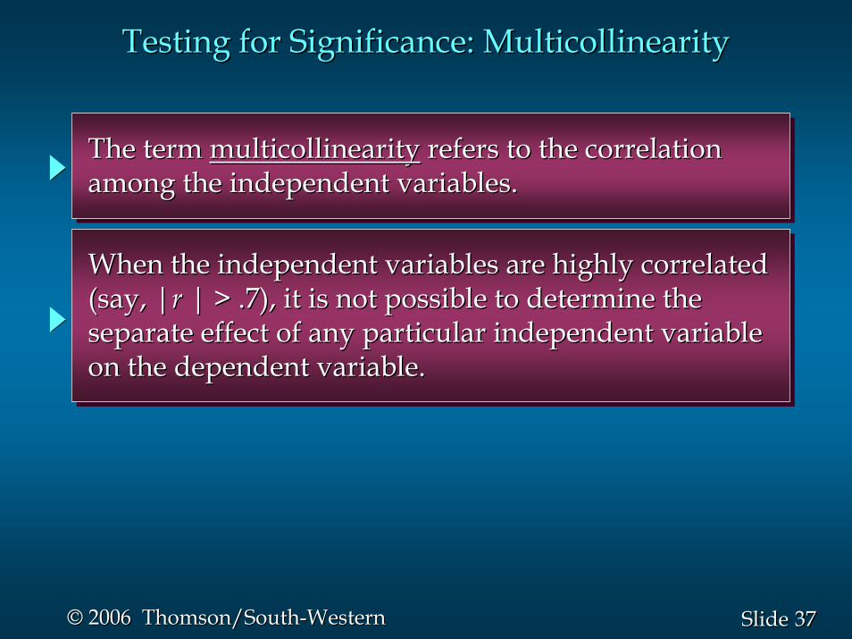
The term multicollinearity refers to the correlationamong the independent variables.The termThe term multicollinearitymulticollinearity refers to the correlationrefers to the correlationamong the independent variables.among the independent variables.
When the independent variables are highly correlated(say, |r | > .7), it is not possible to determine theseparate effect of any particular independent variableon the dependent variable.
When the independent variables are highly correlatedWhen the independent variables are highly correlated(say, |(say, |r r | > .7), it is not possible to determine the| > .7), it is not possible to determine theseparate effect of any particular independent variableseparate effect of any particular independent variableon the dependent variable.on the dependent variable.

3838SlideSlide©© 2006 Thomson/South2006 Thomson/South--WesternWestern
Testing for Significance:Testing for Significance: Multicollinearity Multicollinearity
Every attempt should be made to avoid includingindependent variables that are highly correlated.Every attempt should be made to avoid includingEvery attempt should be made to avoid includingindependent variables that are highly correlated.independent variables that are highly correlated.
If the estimated regression equation is to be used onlyfor predictive purposes, multicollinearity is usuallynot a serious problem.
If the estimated regression equation is to be used onlyIf the estimated regression equation is to be used onlyfor predictive purposes,for predictive purposes, multicollinearitymulticollinearity is usuallyis usuallynot a serious problem.not a serious problem.
3939SlideSlide©© 2006 Thomson/South2006 Thomson/South--WesternWestern
Using the Estimated Regression EquationUsing the Estimated Regression Equationfor Estimation and Predictionfor Estimation and Prediction
The procedures for estimating the mean value of yand predicting an individual value of y in multipleregression are similar to those in simple regression.
The procedures for estimating the mean value of The procedures for estimating the mean value of yyand predicting an individual value of and predicting an individual value of y y in multiplein multipleregression are similar to those in simple regression.regression are similar to those in simple regression.
We substitute the given values of x1, x2, . . . , xp intothe estimated regression equation and use thecorresponding value of y as the point estimate.
We substitute the given values of We substitute the given values of xx11, , xx22, . . . ,, . . . , xxpp intointothe estimated regression equation and use thethe estimated regression equation and use thecorresponding value of corresponding value of yy as the point estimate.as the point estimate.

4040SlideSlide©© 2006 Thomson/South2006 Thomson/South--WesternWestern
Using the Estimated Regression EquationUsing the Estimated Regression Equationfor Estimation and Predictionfor Estimation and Prediction
Software packages for multiple regression will oftenprovide these interval estimates.Software packages for multiple regression will oftenSoftware packages for multiple regression will oftenprovide these interval estimates.provide these interval estimates.
The formulas required to develop interval estimatesfor the mean value of y and for an individual valueof y are beyond the scope of the textbook.
The formulas required to develop interval estimatesThe formulas required to develop interval estimatesfor the mean value of for the mean value of yy and for an individual valueand for an individual valueof of y y are beyond the scope of the textbook.are beyond the scope of the textbook.
^̂̂
4141SlideSlide©© 2006 Thomson/South2006 Thomson/South--WesternWestern
In many situations we must work with qualitativeindependent variables such as gender (male, female),method of payment (cash, check, credit card), etc.
In many situations we must work with In many situations we must work with qualitativequalitativeindependent variablesindependent variables such as gender (male, female),such as gender (male, female),method of payment (cash, check, credit card), etc.method of payment (cash, check, credit card), etc.
For example, x2 might represent gender where x2 = 0indicates male and x2 = 1 indicates female.For example, For example, xx22 might represent gender where might represent gender where xx22 = 0= 0indicates male and indicates male and xx22 = 1 indicates female.= 1 indicates female.
Qualitative Independent VariablesQualitative Independent Variables
In this case, x2 is called a dummy or indicator variable.In this case, In this case, xx22 is called a is called a dummy or indicator variabledummy or indicator variable..
4242SlideSlide©© 2006 Thomson/South2006 Thomson/South--WesternWestern
As an extension of the problem involving theAs an extension of the problem involving thecomputer programmer salary survey, supposecomputer programmer salary survey, supposethat management also believes that thethat management also believes that theannual salary is related to whether theannual salary is related to whether theindividual has a graduate degree inindividual has a graduate degree incomputer science or information systems.computer science or information systems.
The years of experience, the score on the programmerThe years of experience, the score on the programmeraptitude test, whether the individual has a relevant aptitude test, whether the individual has a relevant graduate degree, and the annual salary ($1000) for eachgraduate degree, and the annual salary ($1000) for eachof the sampled 20 programmers are shown on the next of the sampled 20 programmers are shown on the next slide.slide.
Qualitative Independent VariablesQualitative Independent Variables
Example: Programmer Salary SurveyExample: Programmer Salary Survey
4343SlideSlide©© 2006 Thomson/South2006 Thomson/South--WesternWestern
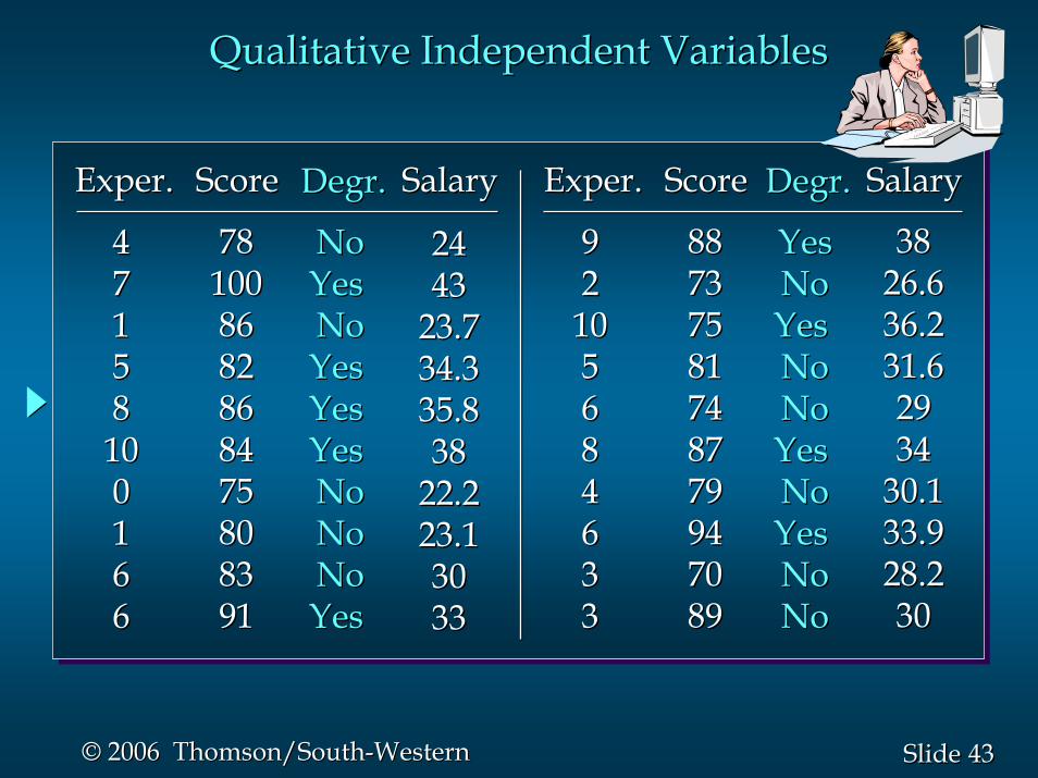
4477115588101000116666
9922101055668844663333
787810010086868282868684847575808083839191
8888737375758181747487877979949470708989
24244343
23.723.734.334.335.835.83838
22.222.223.123.130303333
383826.626.636.236.231.631.629293434
30.130.133.933.928.228.23030
ExperExper.. ScoreScore ScoreScoreExperExper..SalarySalary SalarySalaryDegrDegr..
NoNoYesYesNoNoYesYesYesYesYesYesNoNoNoNoNoNoYesYes
DegrDegr..
YesYesNoNoYesYesNoNoNoNoYesYesNoNoYesYesNoNoNoNo
Qualitative Independent VariablesQualitative Independent Variables
4444SlideSlide©© 2006 Thomson/South2006 Thomson/South--WesternWestern
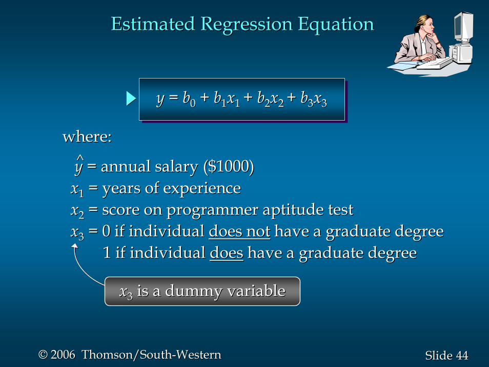
Estimated Regression EquationEstimated Regression Equation
yy = = bb00 + + bb11xx1 1 ++ bb22xx2 2 + + bb33xx33
^̂where:where:
yy = annual salary ($1000)= annual salary ($1000)xx11 = years of experience= years of experiencexx22 = score on programmer aptitude test= score on programmer aptitude testxx33 = 0 if individual = 0 if individual does notdoes not have a graduate degreehave a graduate degree
1 if individual 1 if individual doesdoes have a graduate degreehave a graduate degree
xx33 is a dummy variableis a dummy variable
4545SlideSlide©© 2006 Thomson/South2006 Thomson/South--WesternWestern
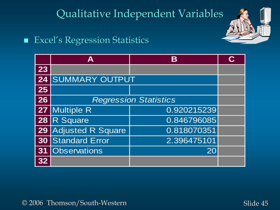
ExcelExcel’’s Regression Statisticss Regression Statistics
A B C23 24 SUMMARY OUTPUT2526 Regression Statistics27 Multiple R 0.92021523928 R Square 0.84679608529 Adjusted R Square 0.81807035130 Standard Error 2.39647510131 Observations 2032
Qualitative Independent VariablesQualitative Independent Variables
4646SlideSlide©© 2006 Thomson/South2006 Thomson/South--WesternWestern
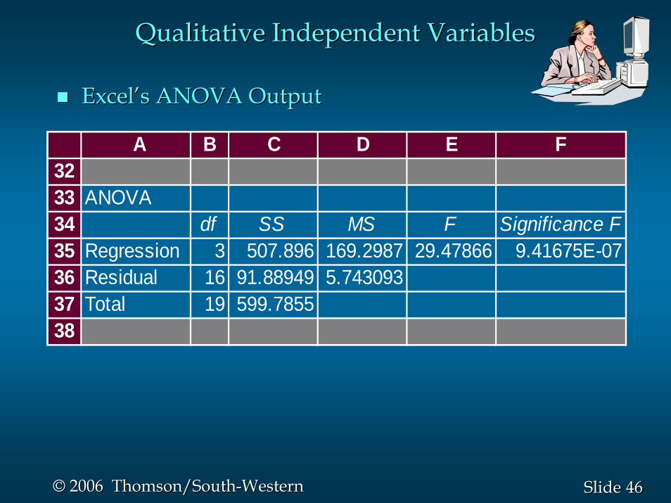
ExcelExcel’’s ANOVA Outputs ANOVA Output
A B C D E F3233 ANOVA34 df SS MS F Significance F35 Regression 3 507.896 169.2987 29.47866 9.41675E-0736 Residual 16 91.88949 5.74309337 Total 19 599.785538
Qualitative Independent VariablesQualitative Independent Variables
4747SlideSlide©© 2006 Thomson/South2006 Thomson/South--WesternWestern
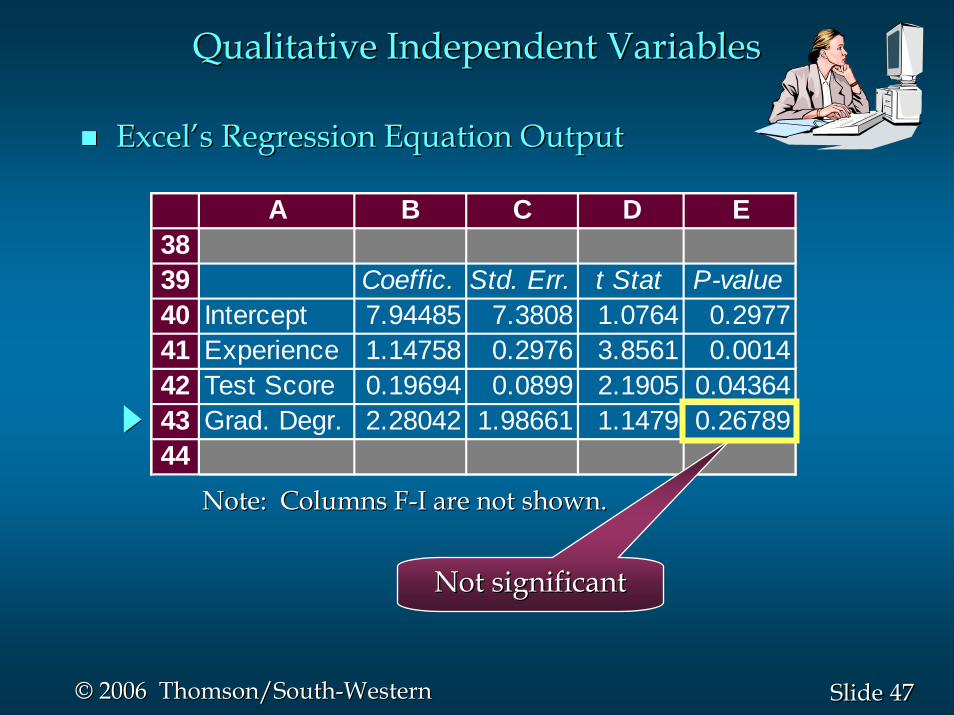
ExcelExcel’’s Regression Equation Outputs Regression Equation Output
A B C D E3839 Coeffic. Std. Err. t Stat P-value40 Intercept 7.94485 7.3808 1.0764 0.297741 Experience 1.14758 0.2976 3.8561 0.001442 Test Score 0.19694 0.0899 2.1905 0.0436443 Grad. Degr. 2.28042 1.98661 1.1479 0.2678944
Note: Columns FNote: Columns F--I are not shown.I are not shown.
Not significantNot significant
Qualitative Independent VariablesQualitative Independent Variables
4848SlideSlide©© 2006 Thomson/South2006 Thomson/South--WesternWestern
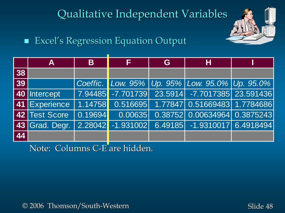
Note: Columns CNote: Columns C--E are hidden.E are hidden.
A B3839 Coeffic.40 Intercept 7.9448541 Experience 1.1475842 Test Score 0.1969443 Grad. Degr. 2.2804244
F G H I
Low. 95% Up. 95% Low. 95.0% Up. 95.0%-7.701739 23.5914 -7.7017385 23.5914360.516695 1.77847 0.51669483 1.77846860.00635 0.38752 0.00634964 0.3875243
-1.931002 6.49185 -1.9310017 6.4918494
ExcelExcel’’s Regression Equation Outputs Regression Equation Output
Qualitative Independent VariablesQualitative Independent Variables
4949SlideSlide©© 2006 Thomson/South2006 Thomson/South--WesternWestern
More Complex Qualitative VariablesMore Complex Qualitative Variables
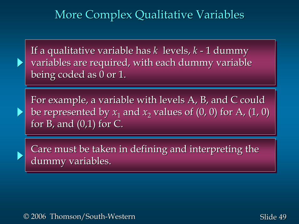
If a qualitative variable has k levels, k - 1 dummyvariables are required, with each dummy variablebeing coded as 0 or 1.
If a qualitative variable has If a qualitative variable has kk levels, levels, kk -- 1 dummy1 dummyvariables are required, with each dummy variablevariables are required, with each dummy variablebeing coded as 0 or 1.being coded as 0 or 1.
For example, a variable with levels A, B, and C couldbe represented by x1 and x2 values of (0, 0) for A, (1, 0)for B, and (0,1) for C.
For example, a variable with levels A, B, and C couldFor example, a variable with levels A, B, and C couldbe represented by be represented by xx11 and and xx22 values of (0, 0) for A, (1, 0)values of (0, 0) for A, (1, 0)for B, and (0,1) for C.for B, and (0,1) for C.
Care must be taken in defining and interpreting thedummy variables.Care must be taken in defining and interpreting theCare must be taken in defining and interpreting thedummy variables.dummy variables.
5050SlideSlide©© 2006 Thomson/South2006 Thomson/South--WesternWestern
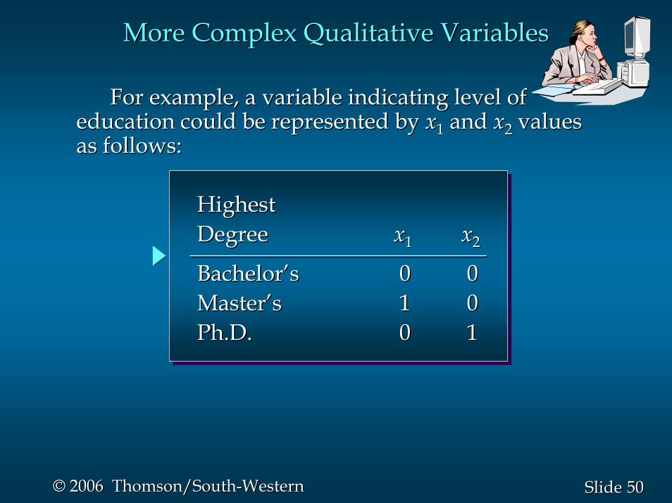
For example, a variable indicating level of For example, a variable indicating level of education could be represented by education could be represented by xx11 and and xx22 values values as follows:as follows:
More Complex Qualitative VariablesMore Complex Qualitative Variables
HighestHighestDegreeDegree xx1 1 xx22
BachelorBachelor’’ss 00 00MasterMaster’’ss 11 00Ph.D.Ph.D. 00 11
5151SlideSlide©© 2006 Thomson/South2006 Thomson/South--WesternWestern
End of Chapter 13End of Chapter 13