Embed Size (px)
Citation preview
University of Coimbra
Faculty of Sciences and Technology
Department of Electrical and Computer Engineering
SLIDING MODE CONTROL APPLIED IN
TRAJECTORY-TRACKING
OF WMRs AND AUTONOMOUS VEHICLES
Razvan Constantin Solea
March 2009

ii
University of Coimbra
Faculty of Sciences and Technology
Department of Electrical and Computer Engineering
SLIDING MODE CONTROL APPLIED IN
TRAJECTORY-TRACKING
OF WMRs AND AUTONOMOUS VEHICLES
A DISSERTATION
SUBMITTED TO THE DEPARTMENT OF
ELECTRICAL AND COMPUTER ENGINEERING
OF COIMBRA UNIVERSITY
IN PARTIAL FULFILLMENT OF THE REQUIREMENTS
FOR THE DEGREE OF DOCTOR OF PHILOSOPHY
Razvan Constantin Solea
UNDER SUPERVISION OF
Professor Urbano NUNES (supervisor)
Professor Adrian FILIPESCU (co-supervisor)

iv
Acknowledgment
I would like to express my deep gratitude to my advisor Prof. Urbano Nunes (Asso-
ciate Professor with the Department of Electrical and Computer Engineering of the
Faculty of Sciences and Technology (FCTUC) of University of Coimbra, Portugal)
for his continuous and patient guidance helping me discover abilities I did not know
I had, for the honest and valuable advises he gave me.
I also want to thank Prof. Adrian Filipescu and Prof. Viorel Dugan (Professors
with the Department of Automation and Industrial Informatics of the Faculty of
Computer Science of University ”Dunarea de Jos” of Galati, Romania) for believing
in me and making this trip possible.
To Elena, thank you for your love, patience, and endless support, especially during
the PhD stage.
To the numerous friends I met in Coimbra, thank you for the funny and not so
funny moments.
During the period of this work, at Institute of Systems and Robotics (ISR) -
Coimbra, Portugal, I was supported in part by Portuguese Foundation for Science
and Technology (FCT), under research fellowship: SFRH/BD//18211/2004 and by
ISR - Coimbra and FCT, under contract NCT04: POSC/EEA/SRI/58016/2004 -
”Nonlinear control techniques applied in path following of WMRs and autonomous,
vehicles with high precision localization system”.
v

vi
Contents
Acknowledgment v
1 Introduction 3
1.1 Motivation and Background . . . . . . . . . . . . . . . . . . . . . . . 3
1.2 Contributions . . . . . . . . . . . . . . . . . . . . . . . . . . . . . . . 5
1.3 Outline of the Thesis . . . . . . . . . . . . . . . . . . . . . . . . . . . 7
2 Trajectory Tracking Problems 9
2.1 Related Works . . . . . . . . . . . . . . . . . . . . . . . . . . . . . . . 9
2.2 Motivation . . . . . . . . . . . . . . . . . . . . . . . . . . . . . . . . . 12
3 Kinematic and Dynamic Models for Differential-drive and Car-like
Mobile Robots 15
3.1 Kinematic and Dynamic Modeling for Differential-drive Robots . . . 15
3.2 Motion Control for WMR . . . . . . . . . . . . . . . . . . . . . . . . 19
3.2.1 Point Stabilization . . . . . . . . . . . . . . . . . . . . . . . . 22
3.2.2 Trajectory Tracking . . . . . . . . . . . . . . . . . . . . . . . . 23
3.2.3 Path Following . . . . . . . . . . . . . . . . . . . . . . . . . . 24
3.3 Kinematic and Dynamic Modeling for Car-like Vehicle . . . . . . . . 27
3.3.1 Dynamics of the Nonlinear Single-Track Model . . . . . . . . . 30
3.3.2 Linearized Single-Track Model . . . . . . . . . . . . . . . . . . 34
3.4 Motion Control for Car-like Vehicle . . . . . . . . . . . . . . . . . . . 36
3.4.1 Longitudinal Control . . . . . . . . . . . . . . . . . . . . . . . 36
3.4.2 Lateral Control . . . . . . . . . . . . . . . . . . . . . . . . . . 37
3.4.3 Integration of Lateral and Longitudinal Controls . . . . . . . . 37
4 Path Planning 39
4.1 Introduction . . . . . . . . . . . . . . . . . . . . . . . . . . . . . . . . 39
vii
4.2 Quintic Equations . . . . . . . . . . . . . . . . . . . . . . . . . . . . . 41
4.3 Velocity Planning . . . . . . . . . . . . . . . . . . . . . . . . . . . . . 43
5 Sliding Mode Control Design 55
5.1 Definitions and Preliminaries . . . . . . . . . . . . . . . . . . . . . . . 55
5.2 Sliding Surface Design . . . . . . . . . . . . . . . . . . . . . . . . . . 58
5.3 Control Law Design . . . . . . . . . . . . . . . . . . . . . . . . . . . . 62
5.4 Chattering Problem and its Reduction . . . . . . . . . . . . . . . . . 67
5.5 Sliding Mode Trajectory-Tracking Control for WMR . . . . . . . . . 69
5.5.1 Simulation Results . . . . . . . . . . . . . . . . . . . . . . . . 71
5.6 Sliding Mode Trajectory-Tracking Control for Car-like Vehicle . . . . 75
5.6.1 Simulation Results . . . . . . . . . . . . . . . . . . . . . . . . 78
5.7 Sliding-Mode Path-Following Control for WMR . . . . . . . . . . . . 80
5.7.1 Simulation Results . . . . . . . . . . . . . . . . . . . . . . . . 83
6 Human Body Comfort 87
6.1 Introduction . . . . . . . . . . . . . . . . . . . . . . . . . . . . . . . . 87
6.2 Model of Human Head-Neck Complex . . . . . . . . . . . . . . . . . . 93
6.3 Experimental Date From Inertial Sensor . . . . . . . . . . . . . . . . 95
7 Implementation in Real Wheelchair - RobChair 99
7.1 Introduction . . . . . . . . . . . . . . . . . . . . . . . . . . . . . . . . 99
7.2 Architecture of RobChair . . . . . . . . . . . . . . . . . . . . . . . . . 101
7.2.1 Hardware and Software Architecture . . . . . . . . . . . . . . 102
7.3 Robot Constraints . . . . . . . . . . . . . . . . . . . . . . . . . . . . 106
7.3.1 Velocity Limits . . . . . . . . . . . . . . . . . . . . . . . . . . 106
7.3.2 Acceleration and Deceleration Limits . . . . . . . . . . . . . . 106
7.3.3 Maximum Velocity to Avoid Sliding Out . . . . . . . . . . . . 107
7.3.4 Wheel-Ground Interaction to Avoid Slippage . . . . . . . . . . 110
7.3.5 Calculation of the Coefficient of Friction . . . . . . . . . . . . 111
7.3.6 Bounded Wheel Speed Commands . . . . . . . . . . . . . . . 112
7.3.7 Dynamic Constraints . . . . . . . . . . . . . . . . . . . . . . . 115
7.3.8 Feasible Constraints . . . . . . . . . . . . . . . . . . . . . . . 116
7.4 Experimental Results . . . . . . . . . . . . . . . . . . . . . . . . . . . 116
7.4.1 Experimental Results Under Odometry Navigation . . . . . . 116
7.4.2 Experimental Results Under Magnetic-markers Navigation . . 117
viii
8 Conclusions 123
A Appendix 125
Bibliography 127
ix

x
List of Tables
3.1 Parameters of the car model . . . . . . . . . . . . . . . . . . . . . . . 31
3.2 Vehicle model summary . . . . . . . . . . . . . . . . . . . . . . . . . 36
4.1 Length, time and r.m.s. acceleration values for each curve . . . . . . 52
4.2 Length, time and r.m.s. acceleration values for each curve (Fig. 4.9) . 54
6.1 Most relevant parameters . . . . . . . . . . . . . . . . . . . . . . . . . 90
6.2 ISO 2631-1 STANDARD. . . . . . . . . . . . . . . . . . . . . . . . . . 92
6.3 Characteristics of user’s elements . . . . . . . . . . . . . . . . . . . . 95
6.4 Experimental results. . . . . . . . . . . . . . . . . . . . . . . . . . . . 96
7.1 Fusion algorithm. . . . . . . . . . . . . . . . . . . . . . . . . . . . . . 105
7.2 Experimental results for SM-TT controller under odometry navigation. 118
7.3 Experimental results for SM-TT controller under odometry navigation. 118
7.4 Experimental results for SM-TT controller under magnetic-markers
navigation. . . . . . . . . . . . . . . . . . . . . . . . . . . . . . . . . . 121
7.5 Experimental results for SM-TT controller under magnetic-markers
navigation. . . . . . . . . . . . . . . . . . . . . . . . . . . . . . . . . . 121
7.6 Experimental results for SM-PF controller under magnetic-markers
navigation. . . . . . . . . . . . . . . . . . . . . . . . . . . . . . . . . . 121
xi

xii
List of Figures
3.1 WMR model and symbols. . . . . . . . . . . . . . . . . . . . . . . . . 16
3.2 Motion control using the kinematic model. . . . . . . . . . . . . . . . 20
3.3 Two-stage model of a real mobile robot. . . . . . . . . . . . . . . . . 20
3.4 Inner loop control of a mobile robot (dynamic-level control). . . . . . 20
3.5 Control of a real mobile robot. . . . . . . . . . . . . . . . . . . . . . . 21
3.6 Description of the Trajectory Tracking Problem. . . . . . . . . . . . . 24
3.7 Description of the Path Following Problem. . . . . . . . . . . . . . . . 25
3.8 Description of the Path Following problem with look-ahead distance. 26
3.9 Kinematics model of A) 4 wheel vehicle; B) Bicycle model. . . . . . . 28
3.10 The one-track bicycle model. . . . . . . . . . . . . . . . . . . . . . . . 32
3.11 The one-track bicycle model. . . . . . . . . . . . . . . . . . . . . . . . 33
4.1 Path planning example using quintic polynomial curves. . . . . . . . . 42
4.2 Lane change (η1 = η2 = 1, 2, 3, 4, 5, η3 = η4 = 0). . . . . . . . . . . . . 44
4.3 Lane change (η1 = η2 = 5, η3 = η4 = −50,−25, 0, 25, 50). . . . . . . . 44
4.4 An example of a longitudinal velocity profile. . . . . . . . . . . . . . . 46
4.5 Restrictive cases of aw. . . . . . . . . . . . . . . . . . . . . . . . . . . 50
4.6 Linear and angular velocity for path example depicted in Fig. 4.1. . . 51
4.7 Lateral and longitudinal accelerations for path example depicted in
Fig. 4.1. . . . . . . . . . . . . . . . . . . . . . . . . . . . . . . . . . . 51
4.8 R.m.s. acceleration values for path example depicted in Fig. 4.1. . . . 52
4.9 Path planning example . . . . . . . . . . . . . . . . . . . . . . . . . . 53
4.10 Linear and angular velocity for path example (Figure 4.9); case A and
B. . . . . . . . . . . . . . . . . . . . . . . . . . . . . . . . . . . . . . 53
4.11 Lateral and longitudinal accelerations for path example (Figure 4.9);
case A and B. . . . . . . . . . . . . . . . . . . . . . . . . . . . . . . . 53
4.12 R.m.s. acceleration values for path example (Figure 4.9); case A and B 54
xiii
5.1 Geometric interpretation of two intersecting switching surfaces. . . . . 57
5.2 Block diagram of observer based sliding mode control. . . . . . . . . . 68
5.3 Disturbance compensation with sliding mode disturbance observer. . 68
5.4 Simulation model block diagram (Simulink scheme). . . . . . . . . . . 72
5.5 Simulink model for RobChair. . . . . . . . . . . . . . . . . . . . . . . 72
5.6 Path examples calculated by the trajectory planner (see Chapter 4). . 72
5.7 Velocities and accelerations for the path depicted in Fig. 5.6. . . . . . 73
5.8 R.M.S. acceleration values for each path-segment (AB, BC,...) of the
paths depicted in Fig. 5.6. . . . . . . . . . . . . . . . . . . . . . . . . 73
5.9 Desired vd, command vc and real vr linear velocities for SM-TT control
- Path 1 and Path 2. . . . . . . . . . . . . . . . . . . . . . . . . . . . 73
5.10 Desired ωd, command ωc and real ωr angular velocities for SM-TT
control - Path1 and Path 2. . . . . . . . . . . . . . . . . . . . . . . . 74
5.11 Desired avd, command avc and real avr longitudinal accelerations for
SM-TT control - Path 1 and Path 2. . . . . . . . . . . . . . . . . . . 74
5.12 Desired aωd, command aωc and real aωr angular accelerations for SM-
TT control - Path1 and Path 2. . . . . . . . . . . . . . . . . . . . . . 74
5.13 Longitudinal, lateral and angular errors of SM-TT control - Path 1 and
Path 2. . . . . . . . . . . . . . . . . . . . . . . . . . . . . . . . . . . . 75
5.14 Simulation SM-TT control starting from an initial error state (xe(0) =
−0.5, ye(0) = −0.5, φe(0) = 0). . . . . . . . . . . . . . . . . . . . . . 75
5.15 Bicycle model (5.62) . . . . . . . . . . . . . . . . . . . . . . . . . . . 76
5.16 Lateral, longitudinal and orientation error (trajectory-tracking) . . . 76
5.17 Simulation model block diagram (Simulink scheme). . . . . . . . . . . 78
5.18 Simulink model for car-like vehicle. . . . . . . . . . . . . . . . . . . . 79
5.19 Desired (vd, δd), command (vc, δd) and real (vr, δr) linear velocities and
steering angles for SM-TT controller without initial pose error - Path
Fig. 4.1 . . . . . . . . . . . . . . . . . . . . . . . . . . . . . . . . . . 79
5.20 Desired (avd, aδd), command (avc, aδc) and real (avr, aδr) longitudinal
and lateral accelerations for SM-TT controller without initial pose error
- Path Fig. 4.1 . . . . . . . . . . . . . . . . . . . . . . . . . . . . . . 79
5.21 Longitudinal (xe), lateral (ye) and orientation (φe) errors for SM-TT
controller without initial pose error - Path Fig. 4.1 . . . . . . . . . . 80
5.22 Simulation SM-TT control starting from an initial error state (xe(0) =
−2.5, ye(0) = −2.5, φe(0) = π/4). . . . . . . . . . . . . . . . . . . . . 80
xiv
5.23 Simulation model block diagram for TT-PF control - Simulink scheme. 84
5.24 Simulation of TT-PF controller with a given longitudinal velocity profile. 84
5.25 Desired aωd, command aωc and real aωr longitudinal and angular ve-
locity for SM-PF control. . . . . . . . . . . . . . . . . . . . . . . . . . 85
5.26 Lateral and angular errors of SM-PF control. . . . . . . . . . . . . . . 85
5.27 Simulation of TT-PF controller with a constant longitudinal velocity
(vd = 0.5m/s). . . . . . . . . . . . . . . . . . . . . . . . . . . . . . . . 85
5.28 Desired aωd, command aωc and real aωr longitudinal and angular ve-
locity for SM-PF control. . . . . . . . . . . . . . . . . . . . . . . . . . 86
5.29 Lateral and angular errors of SM-PF control. . . . . . . . . . . . . . . 86
6.1 The human response (ride quality) involves human variables as well as
dynamic motion and other physical variables, but the ride comfort re-
sponse and technical evaluation of ride (dis-)comfort involves dynamic
motion variables only. Modified from Forstberg [114]. . . . . . . . . . 90
6.2 Human head-neck model . . . . . . . . . . . . . . . . . . . . . . . . . 94
6.3 Experimental sliding-mode trajectory-tracking control using an EKF-
based fusion in the on-line pose estimation. . . . . . . . . . . . . . . . 96
6.4 Cross-spectal density functions for all experiments. . . . . . . . . . . 97
6.5 Longitudinal and lateral accelerations from IMU and from encoders. . 97
7.1 RobChair platform. . . . . . . . . . . . . . . . . . . . . . . . . . . . . 101
7.2 Levels and modules of the motion control system. . . . . . . . . . . . 102
7.3 RobChair CAN-based hardware architecture. . . . . . . . . . . . . . . 103
7.4 Robotic wheelchair model and symbols. . . . . . . . . . . . . . . . . . 106
7.5 Surfaces used in the determination of acceleration limits. . . . . . . . 107
7.6 Experimental (green and red) and desired (blue) wheels speed values
used to determine the maximum acceleration and deceleration of the
RobChair. . . . . . . . . . . . . . . . . . . . . . . . . . . . . . . . . . 108
7.7 Free body diagram showing the RobChair mobile robot (in plane yz). 109
7.8 Free body diagram to find the maximum acceleration before wheel
slippage. . . . . . . . . . . . . . . . . . . . . . . . . . . . . . . . . . . 110
7.9 Schematic showing the forces acting on RobChair to cause it to move. 112
7.10 Feasible WMR velocities. . . . . . . . . . . . . . . . . . . . . . . . . . 113
7.11 Differential drive curvature as function of the wheels speeds. . . . . . 114
7.12 Linear velocity as function of wheels’ speed. . . . . . . . . . . . . . . 115
xv
7.13 Experimental SM-TT control starting from an initial error state (xe(0) =
−1, ye(0) = −1, φe(0) = 0), under odometry navigation. . . . . . . . . 117
7.14 Experimental SM-TT control under magnetic-markers navigation: Left)
Path − 1; Right) Path − 2. In both paths, the circles represent the
positions of the seven magnetic markers used in the experiment. . . . 118
7.15 Experimental SM-PF control under magnetic-markers navigation: Left)
Path − 1; Right) Path − 2. In both paths, the circles represent the
positions of the seven magnetic markers used in the experiment. . . . 119
7.16 RobChair pictures at different positions in a real experiment. . . . . . 119
7.17 Desired (vd, ωd), command (vc, ωc) and real (vr, ωr) linear and angular
velocities for SM-TT control using an EKF-based fusion in the on-line
pose estimation - Path− 1. . . . . . . . . . . . . . . . . . . . . . . . 120
7.18 Desired (vd, ωd), command (vc, ωc) and real (vr, ωr) linear and angular
velocities for SM-TT control using an EKF-based fusion in the on-line
pose estimation - Path− 2. . . . . . . . . . . . . . . . . . . . . . . . 120
7.19 Longitudinal and lateral errors of SM-TT control under magnetic-
markers navigation: Left) Path− 1; Right) Path− 2. . . . . . . . . . 120
7.20 Longitudinal and lateral accelerations from IMU and from encoders in
case of SM-TT control, Left) Path− 1; Right) Path− 2. . . . . . . . 122
xvi
List of Abbreviations
CAN . . . . . . . . . . . . . Controller-Area Network
CSD . . . . . . . . . . . . . Cross Spectral Density
DOF . . . . . . . . . . . . . Degree Of Freedom
EKF . . . . . . . . . . . . . Extended Kalman Filter
eVDV . . . . . . . . . . . . Estimated Vibration Dose Value
FFT . . . . . . . . . . . . . Fast Fourier Transformation
HNC . . . . . . . . . . . . . Head-Neck Complex
IMU . . . . . . . . . . . . . Inertial Measurement Unit
ISO . . . . . . . . . . . . . . International Organization for Standardization
ISR . . . . . . . . . . . . . . Institute of Systems and Robotics
MCL . . . . . . . . . . . . Motion Control Level
MPL . . . . . . . . . . . . . Motion Planning Level
MTL . . . . . . . . . . . . Motion Tracking Level
PSD . . . . . . . . . . . . . Power Spectral Density
rmq . . . . . . . . . . . . . . Root Mean Quad
rms . . . . . . . . . . . . . . Root Mean Square
SM-PF . . . . . . . . . . Sliding-Mode Path-Following
SM-TT . . . . . . . . . . Sliding-Mode Trajectory-Tracking
SMC . . . . . . . . . . . . . Sliding Mode Control
Tr . . . . . . . . . . . . . . . Transmissibility
VDV . . . . . . . . . . . . . Vibration Dose Value
VSC . . . . . . . . . . . . . Variable Structure Control
VSS . . . . . . . . . . . . . Variable Structure Systems
WMR . . . . . . . . . . . . Wheeled Mobile Robot
1

2
Chapter 1
Introduction
1.1 Motivation and Background
Everyday more and more robotic vehicles are entering the real world. They are put to
work just about everywhere manual vehicles have been used in the past. From agri-
culture, and mining operations, to inside factories and hospitals, they are increasing
safety, efficiency, and performance in all tasks otherwise considered to be too dull,
dirty or dangerous for manual labor.
Autonomous vehicles pose a number of unique problems in their design and im-
plementation. There is no longer a human-in-the-loop control scheme for the vehicle.
The system itself must close the loop from environment feedback to low-level vehi-
cle control. Where a human operator would normally analyze data feedback from
telemetry, remote video, etc. and then decide the best course of action, designers
must now instrument the vehicle so that it can automate these tasks. This requires
the inclusion of internal state and environmental sensors, along with onboard com-
puters and software capable of processing the sensed information and planning the
vehicle’s action accordingly.
The first design step is the inclusion of different types of sensors onto the vehicle
platform. These sensors serve two general purposes. The first is to measure the state
of the vehicle itself, such as its position, orientation, speed, and perhaps also health
monitoring information such as comfort, temperature, pressure, etc (proprioception).
The second general purpose is the system’s ability to sense information originating
outside of itself (exteroception). It is the ability to sense one’s environment. Sen-
sors such as cameras and range detectors provide this information. The job of the
system designer is to outfit the autonomous vehicle with those sensors necessary and
3
4 CHAPTER 1. INTRODUCTION
appropriate to provide the correct environment feedback, thus allowing the system to
decide how to act within it.
The second design step is giving the autonomous vehicle the ability to calculate
how to react to sensed internal and external information. This step requires the
vehicle to have the necessary processing and computational power along with the
algorithms and software capable of providing robust and stable control laws that
guide the navigation of the robot.
Autonomous vehicles generate their own decisions, at the planning level, that
govern how to drive the vehicle actuators, and cause the platform to move.
The problem of motion planning and control is that there must be consideration
for the motion constraints of any actuators involved or the vehicle platform itself.
This is especially an important issue for car-like vehicles and WMRs because they are
subject to nonholonomic constraints. This means that a vehicle driving on a surface
may have three degrees of freedom: translation in two dimensions and rotation in
one. Consequently, the equations of motion describing the vehicle dynamics are non-
integrable, which makes the problem much more difficult to solve. This also means
that car-like vehicles and WMRs are under actuated. In other words, the number
of control inputs to the system is less than the number of degrees of freedom in the
system’s configuration space.
Many people nowadays spend a significant proportion of their time travelling and
there is an increasing demand for comfort, in private and public transportation. Three
classes of factors are considered in the analysis of travelling comfort: organizational,
local and riding. The riding comfort can be analysed in three different respects:
dynamic factors - related to vibration, shocks and acceleration; ambient factors -
thermal comfort, air quality, noise, pressure gradients, etc; spatial factors - dealing
with the ergonomics of the passenger’s position.
Comfort is a complex definition that contains both physiological and psychological
components; this includes the subjective feeling of well being with the absence of
discomfort, stress and pain. Comfort not only consists of the absence of negative
effects; it is also the experience of positive aspects of comfort. Therefore, comfort
includes a form of evaluation, i.e. it feels well and has as its opposite, negative
sensations. From interviews of vehicle passengers it is obvious that ride comfort is
dependent not only on the magnitude but also on the occurrence of occasional shocks
or transients.
1.2. CONTRIBUTIONS 5
Ride quality is a person’s reaction to a set of physical conditions in a vehicle envi-
ronment, such as dynamic, ambient and spatial variables. Dynamic variables consist
of motions, measured as accelerations and changes (jerk) in accelerations in all three
axes (lateral, longitudinal and vertical), angular motions about these axes (roll, pitch
and yaw) and sudden motions, such as shocks and jolts. Normally, the axes are fixed
to the vehicle body. The ambient variables may include temperature, pressure, air
quality and ventilation, as well as noise and high frequency vibrations, while the spa-
tial variables may include workspace, leg room and other seating variables. However,
many use the term passenger comfort, ride comfort or average ride comfort for ratings
on a ride quality scale regarding the influence of dynamic variables. Normally, higher
rating on a ride quality scale means better comfort, whereas higher rating on a ride
(dis-)comfort scale means less comfort.
This is the nature of the problem undertaken in this thesis.
The theory of variable structure systems (VSS) opened up a wide new area of de-
velopment for control designers. Variable structure control (VSC), which is frequently
known as sliding mode control (SMC), is characterized by a discontinuous control ac-
tion which changes structure upon reaching a set of predetermined switching surfaces.
This kind of control may result in a very robust system and thus provides a possibility
for achieving our goals. Some promising features of SMC are listed below:
• The order of the motion equation can be reduced.
• The motion equation of the sliding mode can be designed linear and homoge-
nous, despite that the original system may be governed by nonlinear equations.
• The sliding mode does not depend on the process dynamics, but it is determined
by parameters selected by the designer.
• Once the sliding motion occurs, the system has invariant properties which make
the motion independent of certain system parameter variations and distur-
bances. Thus the system performance can be completely determined by the
dynamics of the sliding manifold.
1.2 Contributions
This work has three main contributions:
6 CHAPTER 1. INTRODUCTION
• Although motion planning of mobile robots and autonomous vehicles has been
thoroughly studied in the last decades, the requisite of producing trajectories
with low associated accelerations and jerk is not easily traceable in the techni-
cal literature. This thesis addresses this problem proposing an approach that
consists of introducing a velocity planning stage to generate adequate time se-
quences to be used in the interpolating curve planners. In this context, it is
important to generate speed profiles (linear and angular) that lead to
trajectories respecting human comfort . The need of having travel com-
fort in autonomous vehicle’ applications, motivated my research on the subject
of this thesis.
• In this thesis was proposed a new design of sliding surface for sliding-
mode trajectory-tracking (SM-TT) and sliding-mode path-following
(SM-PF) controller for WMR and car-like vehicle . Due to their non-
holonomic properties, restricted mobility and their relevance in applications,
the trajectory-tracking of those systems has been a challenging class of control
problems. Variable structure control emerges as a robust approach in different
applications and has been successfully applied to control problems as diverse
as automatic flight control, control of electrical motors, regulation in chemical
processes, helicopter stability augmentation, space systems and robotics. One
particular type of VCS system is the sliding mode control methodology. The
theory of SMC has been applied to various control systems, since it has been
shown that this nonlinear type of control exhibits many excellent properties,
such as robustness against large parameter variation and disturbances.
• The transmission of the acceleration to the head-neck complex (HNC) in the
seated human body is a cause of discomfort and motion sickness in vehicles.
The seat back, by limiting the horizontal and rotational motion of the trunk,
increases the transmission of the trunk horizontal acceleration to the HNC.
This may has considerable influence on discomfort. The present thesis ana-
lyzes the comfort of wheelchair users when a SM-TT or a SM-PF
controller is used . The user comfort is examined not only in the time domain
(using the transmissibility parameter), but also in the frequency domain. For
measuring accelerations of the real intelligent wheelchair (platform used in real
experiments), a three-dimensional inertial sensor was used.
1.3. OUTLINE OF THE THESIS 7
Moreover a set of experimental tests using an intelligent wheelchair, called RobChair,
has been performed to evaluate the performance of the SM-TT/SM-PF controller and
the trajectory planning algorithm, with comfort constraint. RobChair prototype has
been developed for allowing experimental studies on rehabilitation applications and
mobility assistance of people with special needs (e.g. people with severely impaired
motion skills), with the purpose of providing them with a certain degree of autonomy
and independence. RobChair is based on a commercial wheelchair, which has been
equipped with an intelligent control system and several sensors.
1.3 Outline of the Thesis
The thesis is structured as follows:
• Chapter 2: Trajectory tracking problems are summarized.
• Chapter 3: Kinematic and dynamic modeling of the WMRs and car-like robots
are presented.
• Chapter 4: The concept of sliding mode are first introduced. Then the funda-
mentals of SMC are summarized, including basic definitions, methods of sliding
surface and control law design, robustness properties and the methods on han-
dling chattering problems. New sliding-mode trajectory-tracking and sliding-
mode path-following controllers for WMRs and car-like vehicles, are also pro-
posed in this chapter.
• Chapter 5: The trajectory/path planning are developed, including the velocity
profile.
• Chapter 6: A model with two freedom degrees is considered for the HNC
model. The user comfort is examined not only in the time domain, but also in
the frequency domain.
• Chapter 7: Experimental results obtained with the implementation of the
proposed controllers in RobChair are summarized and discussed.
• Chapter 8: Finally, conclusions are drawn and some suggestions for future
work are provided.

8 CHAPTER 1. INTRODUCTION
Chapter 2
Trajectory Tracking Problems
2.1 Related Works
Control problems involving mobile robots have attracted considerable attention in the
control community. Most wheeled mobile robots can be classified as nonholonomic
mechanical systems. Controlling such systems is, however, simple. The challenge
presented by these problems comes from the fact that a motion of a wheeled mobile
robot in a plane possesses three degrees of freedom (DOF); while it has to be controlled
using only two control inputs under the nonholonomic constraint.
The methods used in recent years to solve mobile robot control problems can be
classified into three categories. The first category is the sensor-based control ap-
proach to navigation problems. The emphasis is on interactive motion planning in
dynamic environments [1, 2]. Because the working environment for mobile robots
is unstructured and may change with time, the robot must use its on-board sensors
to cope with the dynamic environment. Most reported designs following this ap-
proach rely on intelligent control schemes, such as fuzzy logic control [3, 4, 5] and
neural-network learning control [6, 7]. Obstacle motion estimation and environment
configuration prediction using sensory information are important for proper motion
planning. However, since a mobile robot responds to its surroundings in a reactive or
reflexive way; the executed trajectory may not be globally optimized.
In the second category, the navigation problem is decomposed into a path planning
phase and a path execution phase. A collision- free path is generated and executed
based on a prior map of the environment. The executed path is planned using certain
optimization algorithms based on a minimal time, minimal distance or minimal energy
performance index. Methods for avoiding both static and moving obstacles have been
9
10 CHAPTER 2. TRAJECTORY TRACKING PROBLEMS
reported in the literature [8, 9, 10, 11, 12]. In these methods, a collision-free path is
planned according to the environment map space-time relations. The mobile robot
must follow the planned path employing a path-following controller.
The third category follows the motion control approach, in which a desired trajec-
tory must be tracked accurately. Among these, tracking controller designs employing
a simplified linear model have been reported [13, 14]. In the linear model approach,
however, the controller works only when the linear velocity is not zero. Under such
circumstances, it would be difficult to control the mobile robot to track the specified
trajectory and in the mean time stop with the specified pose. Consequently a more
generalized approach is desirable. Nonlinear system theory has been employed to
solve this problem. Two main research directions employing nonlinear control design
can be distinguished. The first, initiated by Bloch et al. [15], used discontinuous feed-
back, whereas the second research direction used time-varying continuous feedback,
which was first investigated by Samson [16]. Pomet [17] then proposed several smooth
feedback control laws. However, though these solve the regulation problem, they were
found to yield slow asymptotic convergence. In order to obtain faster convergence
(e.g., exponential convergence), an alternative approach was initially proposed by
MCloskey and Murray [18] and taken up in several subsequent studies.
Research on the tracking problem for mobile robots has been extensive. Using
Barbalats lemma or the backstepping method, control schemes have been proposed
for mobile robots to globally follow special paths such as circles and straight lines. In
practical applications, it is preferable to solve the tracking problem and the regulation
problem simultaneously using a single controller; otherwise, switching between two
different types of controllers will be necessary.
Tracking control of nonholonomic mobile robots aims at controlling robots to track
a given time varying trajectory (reference trajectory). It is a fundamental motion
control problem and has been intensively investigated in the robotic community.
Based on whether the system is described by a kinematic model or a dynamic
model, the tracking control problem is classified as either a kinematic or a dynamic
tracking control problem. Several researchers have studied the kinematic tracking
problem and proposed several controllers. Using the kinematic model of WMRs the
trajectory-tracking problem was solved by Kanayama et al. [19]. Both the local and
global tracking problems with exponential convergence have been solved theoretically
using time varying state feedback based on the backstepping technique by Jiang and
Nijmeijer [20].
2.1. RELATED WORKS 11
The kinematic tracking control problem of WMR has been widely studied whereas
dynamic tracking control problem has received attention only recently. Most of the
results on dynamic model based tracking problem of non-holonomic systems are pro-
posed assuming that the kinematics of the system are exactly known and uncertainties
are present only in the dynamics. But practically speaking, uncertainties are present
in both the kinematics and dynamics.
Usually, the reference trajectory is obtained by using a reference (virtual) robot;
therefore, all the kinematic constraints are implicitly considered by the reference
trajectory. The control inputs are mostly obtained by a combination of feedforward
inputs, calculated from reference trajectory, and feedback control law, as in [21, 22,
23]. Lyapunov stable time-varying state-tracking control laws were pioneered by
[19, 16, 24], where the systems equations are linearized with respect to the reference
trajectory, and by defining the desired parameters of the characteristic polynomial
the controller parameters are calculated. The stabilization to the reference trajectory
requires a nonzero motion condition.
A discontinuous stabilizing controller for WMRs with nonholonomic constraints
where the state of the robot asymptotically converges to the target configuration with
a smooth trajectory was presented by Zhang and Hirschorn [25]. A tracking problem
was formulated by Koh and Cho [26] for a mobile robot to follow a virtual target
vehicle that is moved exactly along the path with specified velocity. The driving
velocity control law was designed based on bang-bang control considering the accel-
eration bounds of driving wheels and the robot dynamic constraints in order to avoid
wheel slippage or mechanical damage during navigation. Zhang, et al. [27] employed
a dynamic modeling to design a tracking controller for a differentially steered mobile
robot that is subject to wheel slip and external loads.
Various nonlinear control techniques have been used by many researchers con-
sidering the system disturbances and unknown dynamic parameters. Sliding mode
motion control technique by Yang and Kim [28], robust adaptive control technique
by Kim et al. [29], adaptive control technique by Fukao et al. [30] and higher order
sliding mode technique by Li and Chao [32] have been used to solve the tracking
control problem for WMRs.
A solution for the trajectory tracking problem for a WMR in the presence of distur-
bances that violate the nonholonomic constraint based on discrete-time sliding mode
control [33]. An electromagnetic approach for path guidance of a mobile-robot-based
automatic transport service system with a PD control algorithm was investigated by
12 CHAPTER 2. TRAJECTORY TRACKING PROBLEMS
Wu, et al. [34]. Jiang, et al. [35] developed a model-based control design strategy that
deals with global stabilization and global tracking control for the kinematic model
with a nonholonomic WMR in the presence of input saturations.
Adaptive controls are derived for mobile robots, using backstepping technique, for
tracking of a reference trajectory and stabilization to a fixed posture by Pourboghrat
and Karlsson [36]. In [37], Dong and Kuhnert propose a robust adaptive controller
with the aid of backstepping technique and neural networks.
The trajectory tracking algorithms presented in the above literature share a com-
mon idea of defining velocity control inputs, which stabilize the closed loop system.
In industrial and manufacturing applications, time and speed are very important
parameters when calculating the productivity and efficiency of a process. Hence, in
the trajectory tracking control problem it is a requirement that the WMR be able to
track a time- indexed trajectory. In such cases motion control is commonly achieved
with a velocity profile.
2.2 Motivation
For many years, the control of non-holonomic vehicles has been a very active research
field. At least two reasons account for this fact. On one hand, wheeled vehicles consti-
tute a major and ever more ubiquitous transportation system. Previously restricted to
research laboratories and factories, automated wheeled vehicles are now envisioned
in everyday life (e.g. through car-platooning applications or urban transportation
services), not to mention the military domain.
These novel applications, which require coordination between multiple agents,
give rise to new control problems. On the other hand, the kinematic equations of
non-holonomic systems are highly nonlinear, and thus of particular interest for the
development of nonlinear control theory and practice. Furthermore, some of the
control methods initially developed for non-holonomic systems have proven to be
applicable to other physical systems (e.g. underactuated mechanical systems), as
well as to more general classes of nonlinear systems.
The present thesis addresses sliding-mode control of non-holonomic vehicles, and
more specifically trajectory tracking, by which we mean the problem of stabilizing
the state, or an output function of the state, to a desired reference value, possibly
time-varying.
For controllable linear systems, linear state feedbacks provide, simple, efficient,
2.2. MOTIVATION 13
and robust control solutions. By contrast, for non-holonomic systems, different types
of feedback laws have been proposed, each one carrying its specific advantages and
limitations. As a consequence, the choice of a control approach for a given appli-
cation is a matter of compromise, depending on the system characteristics and the
performance requirements.
In the European Union there are about 80 million elderly or disabled people. Vari-
ous reports also show that there is a strong relation between the age of the person and
the handicaps suffered, the latter being commoner in persons of advanced age. Given
the growth in life expectancy in the EU, this means that a large part of its popula-
tion will experience functional problems. Aware of the dearth of applications for this
sector of the population, governments and public institutions have been promoting
research in this line in this recent years. Various types of research groups at a world
level have begun to set up cooperation projects, projects to aid communication and
mobility of elderly and/or disabled persons with the aim of increasing their quality
of life and allowing them a more autonomous and independent lifestyle and greater
chances of social integration.
One of the most potentially useful applications for increasing the mobility of dis-
abled and/or elderly persons is wheelchair implementation. A standard motorized
wheelchair aids the mobility of disabled people who cannot walk, always providing
that their disability allows them to control the joystick safely. Persons with a seri-
ous disability or handicap, however, may find it difficult or impossible to use them;
cases in point could be tetraplegics who are capable only of handling an onoff sensor
or make certain very limited movements. This would make control of the wheelchair
particularly difficult, especially on delicate manoeuvres. For such cases it is necessary
to develop more complex human-wheelchair interfaces adapted to the disability of the
user, thus allowing them to input movement commands in a safe and simple way.
14 CHAPTER 2. TRAJECTORY TRACKING PROBLEMS
Chapter 3
Kinematic and Dynamic Models
for Differential-drive and Car-like
Mobile Robots
In this section, a review of modeling and control of nonholonomic mobile robots is
provided. In such robots, the motion control will be subject to nonholonomic con-
straints, which make motion perpendicular to the wheels impossible. This constraint
involves a nontrivial control method although the full state be measured.
3.1 Kinematic and Dynamic Modeling for Differential-
drive Robots
A mobile robot system having an n-dimensional configuration space with generalized
variables (q1, q2, ..., qn) and subject to constraints can be described by [38]:
M(q) · q + Vm(q, q) · q + F (q) +G(q) + τd = B(q) · τ − AT (q) · λ (3.1)
where M(q) ∈ Rn×n is a symmetric, positive definite inertia matrix, Vm(q, q) ∈ Rn×n
is the centripetal and Coriolis matrix, F (q) ∈ Rn×1 denotes the surface friction,
G(q) ∈ Rn×1 is the gravitational vector, τd denotes bounded unknown disturbances
including unstructured unmodeled dynamics, B(q) ∈ Rn×r is the input transforma-
tion matrix, τ ∈ Rn×1 is the input vector, A(q) ∈ Rm×n is the matrix associated with
the constraints, and, λ ∈ Rm×1 is the vector of constraint forces. The nonholonomic
15
16 CHAPTER 3. KINEMATIC AND DYNAMIC MODELS
nature of a mobile robot is related to the assumption that the wheels of the vehi-
cle roll without skidding. They are subject to non-integrable equality nonholonomic
constraints involving the velocity. In other words, the dimension of the admissible ve-
locity space is smaller than the dimension of the configuration space. This constraint
can be written as:
A(q) · q = 0 (3.2)
In the case of a differential-drive WMR, the model used in [30] and [31] is used in
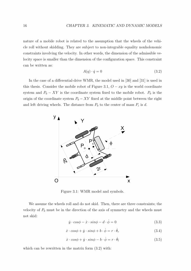
this thesis. Consider the mobile robot of Figure 3.1, O − xy is the world coordinate
system and P0 − XY is the coordinate system fixed to the mobile robot. P0 is the
origin of the coordinate system P0−XY fixed at the middle point between the right
and left driving wheels. The distance from P0 to the center of mass Pc is d.
Figure 3.1: WMR model and symbols.
We assume the wheels roll and do not skid. Then, there are three constraints; the
velocity of P0 must be in the direction of the axis of symmetry and the wheels must
not skid:
y · cosφ− x · sinφ− d · φ = 0 (3.3)
x · cosφ+ y · sinφ+ b · φ = r · θr (3.4)
x · cosφ+ y · sinφ− b · φ = r · θl (3.5)
which can be rewritten in the matrix form (3.2) with:
3.1. KINEMATIC AND DYNAMIC MODELING FOR ROBOTS 17
A(q) =
sinφ −cosφ d 0 0
cosφ sinφ b −r 0
cosφ sinφ −b 0 −r
The system (3.1) can be rewritten as follows:
M(q) · q + Vm(q, q) · q = B(q) · τ − AT (q) · λ (3.6)
For the later description, mc is the mass of the robot’s body and mw is the mass
of a driving wheel plus its associated motor; Ic, Iw, and Im are the moment of inertia
of the body about the vertical axis through Pc, the wheel with a motor about the
wheel axis, and the wheel with a motor about the wheel diameter, respectively. The
matrices M , Vm and B are given by:
M(q) =
m 0 2 ·mw · d · sinφ 0 0
0 m −2 ·mw · d · cosφ 0 0
2 ·mw · d · sinφ −2 ·mw · d · cosφ I 0 0
0 0 0 Iw 0
0 0 0 0 Iw
Vm(q, q) =
2 ·mw · d · φ2 · cosφ
2 ·mw · d · φ2 · sinφ
0
0
0
, B(q) =
0 0
0 0
0 0
1 0
0 1
, τ =
τr
τl
Where I and m are given by: I = mc · d2 + Ic + 2 ·mw · b
2 + 2 · Im, m = mc + 2 ·mw.
Five generalized coordinates can describe the configuration of the mobile robot:
q = [x, y, φ, θr, θl]T , where (x, y) are the coordinates of P0, φ is the heading angle of
the mobile robot, and θr,θl are the angles of the right and left driving wheels.
Let S(q) be a full rank matrix formed by a set of smooth and linearly independent
vectors such as:
ST (q) · AT (q) = 0 (3.7)
It is easy to verify that S(q) is given by:
18 CHAPTER 3. KINEMATIC AND DYNAMIC MODELS
S(q) =
r2·b· (b · cosφ− d · sinφ) r
2·b· (b · cosφ+ d · sinφ)
r2·b· (b · sinφ+ d · cosφ) r
2·b· (b · sinφ− d · cosφ)
r2·b
− r2·b
1 0
0 1
According to (3.1) and (3.7), it is possible to find that:
q = S(q) · ν (3.8)
where ν = [ν1 ν2] whose elements are the angular velocities of the right and left
wheels. Equation (3.8) represents the kinematic model of the robot. Differentiating
(3.8), substituting the result in (3.1), and then multiplying by ST , we can eliminate
the constraint matrix AT (q) · λ. Also, if we denote M = ST · M · S and V m =
ST ·(
M · S + Vm · S)
, and after simplifications, the nonholonomic mobile robot model
(3.1) can be written in the form of:
M(q) · ν + V m(q, q) · ν = B(q) · τ (3.9)
where
M(q) =
r2
4·b2· (m · b2 + I) + Iw
r2
4·b2· (m · b2 − I)
r2
4·b2· (m · b2 − I) r2
4·b2· (m · b2 + I) + Iw
V m =
0 r2
2·b·mc · d · φ
− r2
2·b·mc · d · φ 0
, B =
1 0
0 1
, τ =
τr
τl
Equations (3.8) and (3.9) represent the kinematic and dynamic models of the
robot, respectively. From equation (3.8) we can obtain that:
d
dt
x
y
φ
θr
θl
=
r2· cosφ r
2· cosφ
r2· sinφ r
2· sinφ
r2·b
− r2·b
1 0
0 1
·
ν1
ν2
(3.10)
The relation between (v, w) and (ν1, ν2) is:
ν1
ν2
=
1r
br
1r− b
r
·
v
ω
(3.11)
3.2. MOTION CONTROL FOR WMR 19
where v and ω are the linear and angular velocity of the robot. If we want to focus
only on x, y, and φ then it is sufficient to substitute (3.11) in (3.10). We will get the
ordinary form of a mobile robot with two actuated wheels:
d
dt
x
y
φ
=
cosφ 0
sinφ 0
0 1
·
v
ω
(3.12)
3.2 Motion Control for WMR
Motion control of mobile robots has been studied by many authors in the last decade,
since they are increasingly used in wide range of applications. At the beginning, the
research effort was focused only on the kinematic model, assuming that there is per-
fect velocity tracking [38]. The main objective was to find suitable velocity control
inputs, which stabilize the kinematic closed loop control. Later on, the research was
conducted to design motion controllers, including also the dynamics of the robot.
However, when the dynamics part is considered, exact knowledge about the param-
eters values of the mobile robot is almost unattainable in practice. If we consider
that during the robot motion, these parameters may change due to surface friction,
additional load, among others, the problem becomes more complicated. Furthermore,
the control at the kinematic level may be unstable if there are control errors at the
dynamic level. Therefore, the control at the dynamic level is at least as important
as the kinematic-level control. At present, PID controllers are still widely used in
motor control of mobile robots and in industrial control systems in general. However,
its ability to cope with some complex process properties such as non-linearities, and
time-varying parameters is known to be very poor. Recently, some investigations
have been conducted to design non-linear dynamic controllers. Instead of using ap-
proximate linear models as in the design of conventional linear controllers, non-linear
models are used and non-linear feedbacks are employed on the control loop. Using
non-linear controllers, system stability can be improved significantly; a few results
are available in [30] and [39]. However, nonlinear controllers have a more complicated
structure, and are more difficult to find and to implement.
In motion control, the objective is to control the velocity of the robot such that its
pose P = [x, y, φ]T follows a reference trajectory Pr = [xr, yr, φr]T . At the beginning,
the research effort was focused only on the kinematic model, assuming that there
is perfect velocity tracking. Thus, the controllers neglect the vehicle dynamics and
20 CHAPTER 3. KINEMATIC AND DYNAMIC MODELS
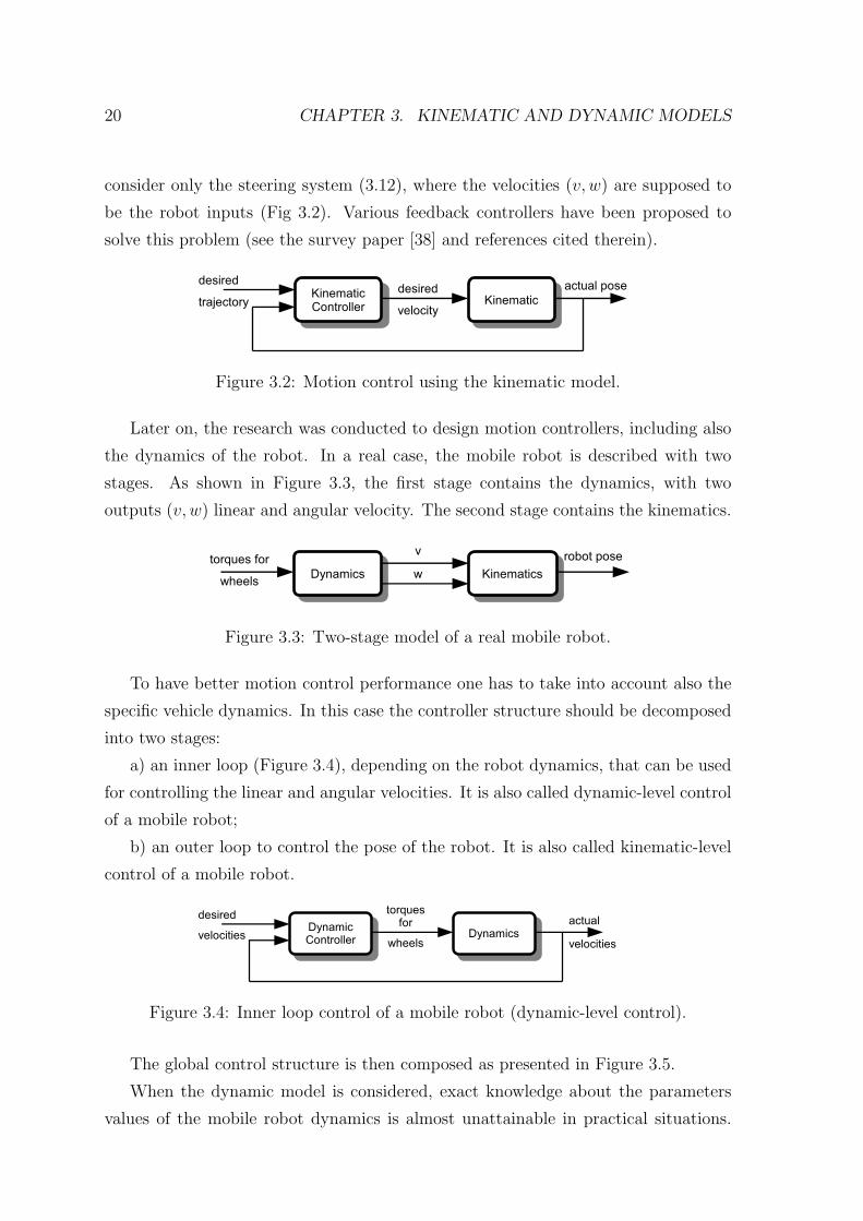
consider only the steering system (3.12), where the velocities (v, w) are supposed to
be the robot inputs (Fig 3.2). Various feedback controllers have been proposed to
solve this problem (see the survey paper [38] and references cited therein).
Figure 3.2: Motion control using the kinematic model.
Later on, the research was conducted to design motion controllers, including also
the dynamics of the robot. In a real case, the mobile robot is described with two
stages. As shown in Figure 3.3, the first stage contains the dynamics, with two
outputs (v, w) linear and angular velocity. The second stage contains the kinematics.
Figure 3.3: Two-stage model of a real mobile robot.
To have better motion control performance one has to take into account also the
specific vehicle dynamics. In this case the controller structure should be decomposed
into two stages:
a) an inner loop (Figure 3.4), depending on the robot dynamics, that can be used
for controlling the linear and angular velocities. It is also called dynamic-level control
of a mobile robot;
b) an outer loop to control the pose of the robot. It is also called kinematic-level
control of a mobile robot.
Figure 3.4: Inner loop control of a mobile robot (dynamic-level control).
The global control structure is then composed as presented in Figure 3.5.
When the dynamic model is considered, exact knowledge about the parameters
values of the mobile robot dynamics is almost unattainable in practical situations.
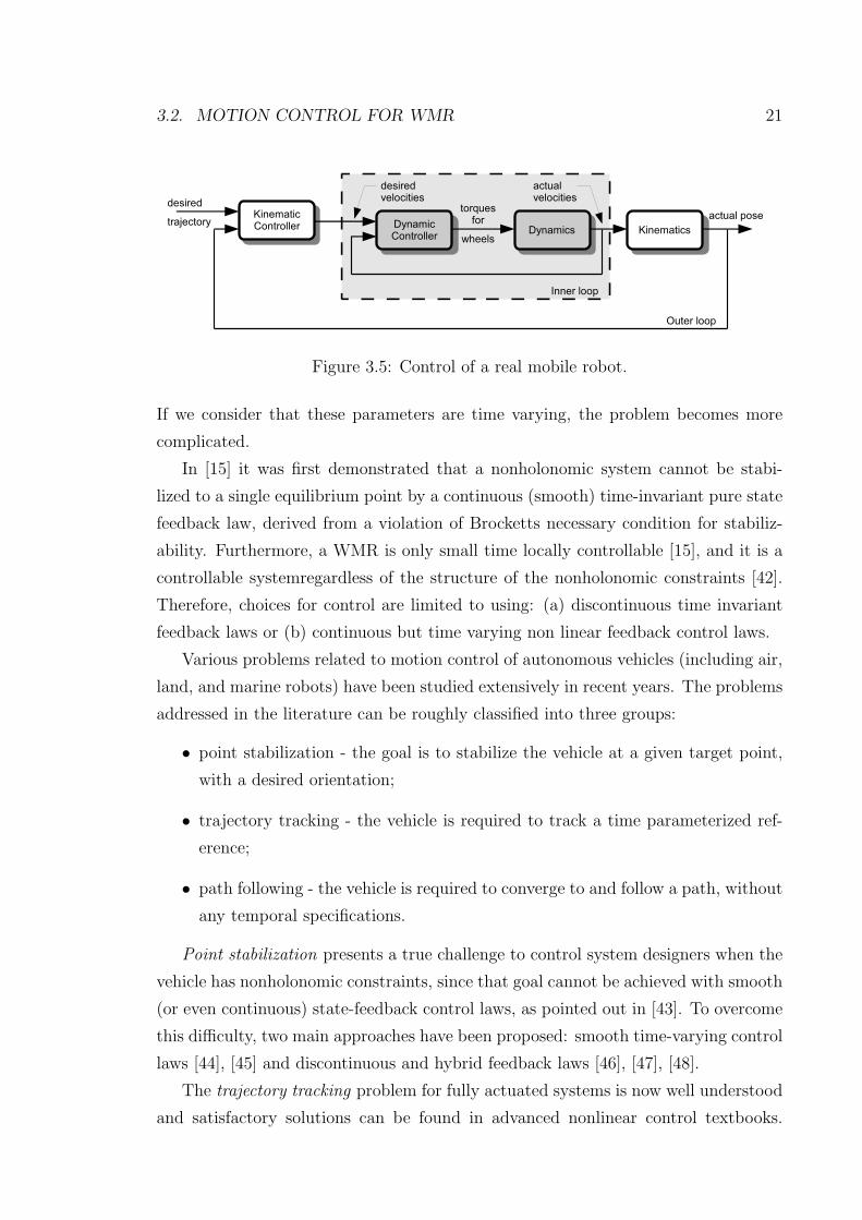
3.2. MOTION CONTROL FOR WMR 21
Figure 3.5: Control of a real mobile robot.
If we consider that these parameters are time varying, the problem becomes more
complicated.
In [15] it was first demonstrated that a nonholonomic system cannot be stabi-
lized to a single equilibrium point by a continuous (smooth) time-invariant pure state
feedback law, derived from a violation of Brocketts necessary condition for stabiliz-
ability. Furthermore, a WMR is only small time locally controllable [15], and it is a
controllable systemregardless of the structure of the nonholonomic constraints [42].
Therefore, choices for control are limited to using: (a) discontinuous time invariant
feedback laws or (b) continuous but time varying non linear feedback control laws.
Various problems related to motion control of autonomous vehicles (including air,
land, and marine robots) have been studied extensively in recent years. The problems
addressed in the literature can be roughly classified into three groups:
• point stabilization - the goal is to stabilize the vehicle at a given target point,
with a desired orientation;
• trajectory tracking - the vehicle is required to track a time parameterized ref-
erence;
• path following - the vehicle is required to converge to and follow a path, without
any temporal specifications.
Point stabilization presents a true challenge to control system designers when the
vehicle has nonholonomic constraints, since that goal cannot be achieved with smooth
(or even continuous) state-feedback control laws, as pointed out in [43]. To overcome
this difficulty, two main approaches have been proposed: smooth time-varying control
laws [44], [45] and discontinuous and hybrid feedback laws [46], [47], [48].
The trajectory tracking problem for fully actuated systems is now well understood
and satisfactory solutions can be found in advanced nonlinear control textbooks.
22 CHAPTER 3. KINEMATIC AND DYNAMIC MODELS
However, in the case of underactuated vehicles, that is, when the vehicles have less
actuators than state variables to be tracked, the problem is still a very active topic
of research. Linearization and feedback linearization methods [49], [50] as well as
Lyapunov based control laws [44], [51] have been proposed.
Path following control has received relatively less attention in the literature. See
[52], [53] for pioneering work in the area as well as [44], [54] and the references therein.
The underlying assumption in path following control is that the vehicles forward speed
tracks a desired speed profile, while the controller acts on the vehicle orientation to
drive it to the path. Typically, smoother convergence to a path is achieved (when
compared to the behaviour obtained with trajectory tracking control laws) and the
control signals are less likely pushed to saturation.
3.2.1 Point Stabilization
The challenge is that nonholonomic mobile robot systems have more degrees of free-
dom than controls. When represented in Cartesian space, they cannot be stabilized
with a continuously differentiable, time-invariant feedback control law as pointed out
in the famous paper by Brockett [43]. Various approaches have been undertaken
to stabilize these systems such as time-varying [63], adaptive [55], [37] discontinuous
[56], and neural network based [57] strategies. For a thorough survey of nonholonomic
control techniques see the review in [39].
The various strategies may be broken up into three basic types: discontinuous
time-invariant, continuous time-varying, and hybrid techniques that are some com-
bination of the other two. All of the techniques make use of the fact that Brocketts
Theorem shows that feedback stabilization is achievable if there is a discontinuity
introduced in either the control law or time.
Discontinuous time-invariant techniques are of two basic types: piecewise contin-
uous and sliding mode controllers. Sliding mode controllers can provide good con-
vergence rates by forcing the trajectory to slide on a manifold towards equilibrium,
but often have problems with chatter as the controller switches control laws along the
manifold. Piecewise continuous controllers are of several types, but most make use of
a coordinate transformation introducing a discontinuity at the origin [58], [59], [60].
These controllers offer exponential convergence rates without the problem of chatter
experienced by sliding mode control, and generally produce smooth natural looking
paths [61].
3.2. MOTION CONTROL FOR WMR 23
The time-varying control laws that have been developed generally suffer from two
problems. Firstly, since time is discontinuous, exponential convergence usually cannot
be guaranteed. Hence, these controllers normally suffer from slow convergence rates
[39]. Second, the paths generated by this type of controller are generally not smooth
or natural looking. They would require a robot with a high degree of maneuverability
to follow the generated paths. Most of the hybrid techniques also suffer from these
two problems.
Many of the proposed techniques make the simplifying assumption that the mobile
robot is a simple unicycle vehicle type. These techniques are therefore well suited to
vehicles with only one axle to control, the ability to perform a zero radius turn, and
easily reverse direction.
3.2.2 Trajectory Tracking
Trajectory tracking (TT) has been well studied because it is similar to servosystems,
and it is guaranteed that the system will converge to the desired trajectory in a deter-
ministic time using an asymptotically stable control law (except for the perturbations
that it may suffer). On the other hand, path following (PF) is not well suited for sys-
tems with strict timing requirements, but it is very suitable for nonholonomic systems
and is applicable to many mobile robots since they are not usually involved in hard
real-time systems. Although the first approach seems to be the most straightforward,
it has been shown that the second is more suitable for many situations in which time
is not a critical parameter.
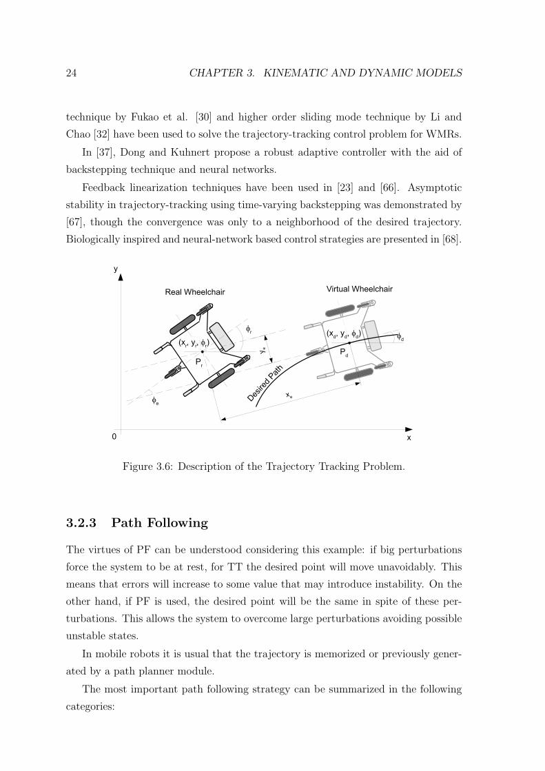
This is the case for most applications in mobile industrial robots or assistant robots
such as computerized wheelchairs (see Fig 3.6). This situation can be understood if we
consider the following example in TT systems: if big perturbations force the system
to be at rest, the desired point for trajectory tracking will move unavoidably. This
means that errors will increase to some value that may introduce instability. On
the other hand, if PF were used, the desired point will be the same despite these
perturbations, because the paths shape and the real robot state remain the same.
This allows the system to overcome large perturbations, avoiding possible unstable
states. Thus interest in PF for mobile robots is rapidly growing.
Sliding-mode controllers have been devised by [65] for holonomic robots and ex-
tended for nonholonomic robots. Sliding-mode motion control technique by Yang
and Kim [28], robust adaptive control technique by Kim et al. [29], adaptive control
24 CHAPTER 3. KINEMATIC AND DYNAMIC MODELS
technique by Fukao et al. [30] and higher order sliding mode technique by Li and
Chao [32] have been used to solve the trajectory-tracking control problem for WMRs.
In [37], Dong and Kuhnert propose a robust adaptive controller with the aid of
backstepping technique and neural networks.
Feedback linearization techniques have been used in [23] and [66]. Asymptotic
stability in trajectory-tracking using time-varying backstepping was demonstrated by
[67], though the convergence was only to a neighborhood of the desired trajectory.
Biologically inspired and neural-network based control strategies are presented in [68].
Figure 3.6: Description of the Trajectory Tracking Problem.
3.2.3 Path Following
The virtues of PF can be understood considering this example: if big perturbations
force the system to be at rest, for TT the desired point will move unavoidably. This
means that errors will increase to some value that may introduce instability. On the
other hand, if PF is used, the desired point will be the same in spite of these per-
turbations. This allows the system to overcome large perturbations avoiding possible
unstable states.
In mobile robots it is usual that the trajectory is memorized or previously gener-
ated by a path planner module.
The most important path following strategy can be summarized in the following
categories:
3.2. MOTION CONTROL FOR WMR 25
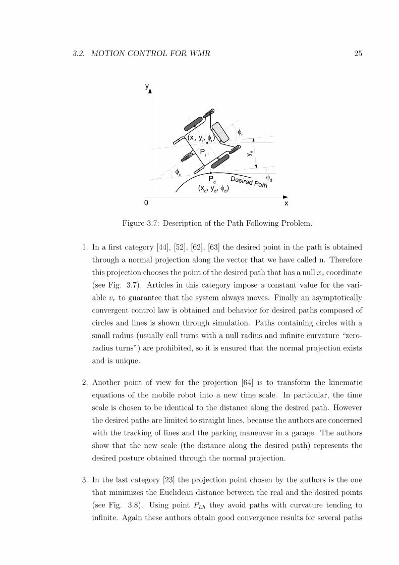
Figure 3.7: Description of the Path Following Problem.
1. In a first category [44], [52], [62], [63] the desired point in the path is obtained
through a normal projection along the vector that we have called n. Therefore
this projection chooses the point of the desired path that has a null xe coordinate
(see Fig. 3.7). Articles in this category impose a constant value for the vari-
able vr to guarantee that the system always moves. Finally an asymptotically
convergent control law is obtained and behavior for desired paths composed of
circles and lines is shown through simulation. Paths containing circles with a
small radius (usually call turns with a null radius and infinite curvature “zero-
radius turns”) are prohibited, so it is ensured that the normal projection exists
and is unique.
2. Another point of view for the projection [64] is to transform the kinematic
equations of the mobile robot into a new time scale. In particular, the time
scale is chosen to be identical to the distance along the desired path. However
the desired paths are limited to straight lines, because the authors are concerned
with the tracking of lines and the parking maneuver in a garage. The authors
show that the new scale (the distance along the desired path) represents the
desired posture obtained through the normal projection.
3. In the last category [23] the projection point chosen by the authors is the one
that minimizes the Euclidean distance between the real and the desired points
(see Fig. 3.8). Using point PLh they avoid paths with curvature tending to
infinite. Again these authors obtain good convergence results for several paths
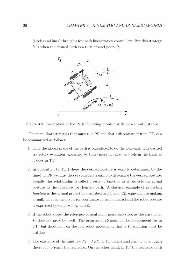
26 CHAPTER 3. KINEMATIC AND DYNAMIC MODELS
(circles and lines) through a feedback linearization control law. But this strategy
fails when the desired path is a turn around point Pr.
Figure 3.8: Description of the Path Following problem with look-ahead distance.
The main characteristics that must rule PF and that differentiate it from TT, can
be summarized as follows:
1. Only the global shape of the path is considered to do the following. The desired
trajectory evolution (governed by time) must not play any role in the track as
it does in TT.
2. In opposition to TT (where the desired posture is exactly determined by the
time), in PF we must choose some relationship to determine the desired posture.
Usually this relationship is called projecting function as it projects the actual
posture to the reference (or desired) path. A classical example of projecting
function is the normal projection described in [44] and [52], equivalent to making
ex null. That is, the first error coordinate xe, is eliminated and the robot posture
is expressed by only two: ye and φe.
3. If the robot stops, the reference or goal point must also stop, as the parameter
Pd does not grow by itself. The progress of Pd must not be independent (as in
TT) but dependent on the real robot movement, that is Pd equation must be
driftless.
4. The existence of the rigid law Pd = Pd(t) in TT understand pulling or dragging
the robot to reach the reference. On the other hand, in PF the reference path
3.3. KINEMATIC AND DYNAMIC MODELING FOR CAR-LIKE VEHICLE 27
can not pull (or drag) the robot: the robot must move independently by some
condition (of course, meanwhile a control law must ensure convergence to the
path). We must impose a motion in the real system to guarantee that it moves
or progresses. In the current mobile robot literature most motion exigencies
are applied to WMR robots, so it is usual to have vd = ct (other authors use
|vd| 6= 0) or a velocity profile for vd is supposed to be given between the initial
and final position.
5. A direct result of what is explained before is that there is no time exigency in
the following. This means that we cannot ensure that the robot will reach a
reference point in a predictable period of time.
3.3 Kinematic and Dynamic Modeling for Car-like
Vehicle
A nonholonomic kinematic model of a vehicle is tackled in this section. The sideslip of
the vehicle and lateral slips of the wheels are taken into account while discussing the
nonholonomic constraints. To discuss a nonholonomic kinematic model of a vehicle,
the following assumptions are considered: a) distances between wheels (generally
called as wheelbase or tread) are strictly fixed; b) the steering axle of each wheel is
perpendicular to a surface terrain; c) a vehicle does not consist of any flexible parts.
A kinematic model of vehicle including the lateral slips is shown in Fig. 3.9A.
In this model, each wheel has a certain steering angle δi and slip angle βi. The slip
angle, which defines how large the wheel generates the lateral slip, is calculated by
the longitudinal and lateral linear velocities vxwi, vywi
of the wheel as follows:
βi = tan−1
(
vywi
vxwi
)
(3.13)
The subscript i denotes each wheel ID as shown in Fig. 3.9A. (xCG, yCG, ψ)
defines the position and an orientation of the center of gravity of the vehicle (CG),
while (xwi, ywi) defines the position of the i− th wheel. v and vi are linear velocities
of the vehicle and each wheel, respectively. Also, β denotes the sideslip of the vehicle,
which is determined by a similar equation of (3.13). lf and lr means the longitudinal
distance from the center of gravity of the vehicle to the front or rear wheels and d
defines the wheelbase. Here, based on the assumption as previously pointed, lf , lr
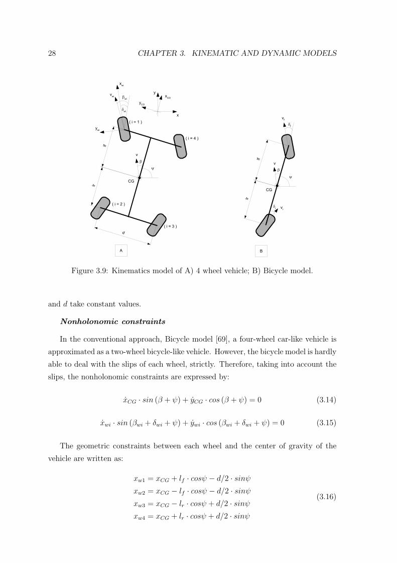
28 CHAPTER 3. KINEMATIC AND DYNAMIC MODELS
Figure 3.9: Kinematics model of A) 4 wheel vehicle; B) Bicycle model.
and d take constant values.
Nonholonomic constraints
In the conventional approach, Bicycle model [69], a four-wheel car-like vehicle is
approximated as a two-wheel bicycle-like vehicle. However, the bicycle model is hardly
able to deal with the slips of each wheel, strictly. Therefore, taking into account the
slips, the nonholonomic constraints are expressed by:
xCG · sin (β + ψ) + yCG · cos (β + ψ) = 0 (3.14)
xwi · sin (βwi + δwi + ψ) + ywi · cos (βwi + δwi + ψ) = 0 (3.15)
The geometric constraints between each wheel and the center of gravity of the
vehicle are written as:
xw1 = xCG + lf · cosψ − d/2 · sinψ
xw2 = xCG − lf · cosψ − d/2 · sinψ
xw3 = xCG − lr · cosψ + d/2 · sinψ
xw4 = xCG + lr · cosψ + d/2 · sinψ
(3.16)
3.3. KINEMATIC AND DYNAMIC MODELING FOR CAR-LIKE VEHICLE 29
yw1 = yCG + lf · sinψ + d/2 · cosψ
yw2 = yCG − lf · sinψ + d/2 · cosψ
yw3 = yCG − lr · sinψ − d/2 · cosψ
yw4 = yCG + lr · sinψ − d/2 · cosψ
(3.17)
Substituting equations (3.16) and (3.17) by equation (3.15), the following matrix
form equation is obtained:
A0 · q0 = 0 (3.18)
where
A0 =
sinφw1 −cosφw1 −lf · cos (φw1 − ψ)− d/2 · sin (φw1 − ψ)
sinφw2 −cosφw2 lr · cos (φw2 − ψ) + d/2 · sin (φw2 + ψ)
sinφw3 −cosφw3 lr · cos (φw3 − ψ)− d/2 · sin (φw3 + ψ)
sinφw4 −cosφw4 −lf · cos (φw4 − ψ) + d/2 · sin (φw4 − ψ))
sinφ0 −cosφ0 0
q0 =
xCG
yCG
ψ
= 0
(3.19)
where φ0 = β + ψ, φwi = βwi + δwi + ψ, i = 1, 2, 3, 4.
Here, it is complicated to derive a null-space vector of the constraints matrix
A0 if obtaining the vector q0 which satisfies equation (3.18). Therefore, a simplified
constrains matrix A12 for bicycle model (Figure 3.9B) is represented instead of A0.
For instance, in terms of a bicycle model (i = 1, 2):
A12 · q0 = 0 (3.20)
where
A12 =
sinφw1 −cosφw1 −lf · cos (φw1 − ψ)− d/2 · sin (φw1 − ψ)
sinφw2 −cosφw2 lr · cos (φw2 − ψ) + d/2 · sin (φw2 + ψ)
sinφ0 −cosφ0 0
q0 =
xCG
yCG
ψ
= 0
(3.21)
Under the basic assumptions of planar motion, rigid body and non-slippage of
30 CHAPTER 3. KINEMATIC AND DYNAMIC MODELS
tire, the four-wheel vehicle can be approximated by a bicycle model, as shown in
Figure 3.9. To describe the vehicle motion, a global coordinate x− y is fixed on the
horizontal plane on which the vehicle moves. The motion status of the vehicle can be
described using the bicycle model as illustrated in Figure 3.9B.
sin (δf + ψ) −cos (δf + ψ) −lf · cosδf
sin (δr + ψ) −cos (δr + ψ) lr · cosδr
sin (β + ψ) −cos (β + ψ) 0
·
xCG
yCG
ψ
= 0 (3.22)
Using a null-space vector of A12, it is possible to obtain the vector q0 satisfying
equation (3.22):
xCG
yCG
ψ
=
cos (β + ψ)
sin (β + ψ)cosβ·(tanδf−tanδr)
lf+lr
· v (3.23)
where β = arctanlf ·tanδr+lr·tanδf
lf+lrand v is linear velocity of the vehicle.
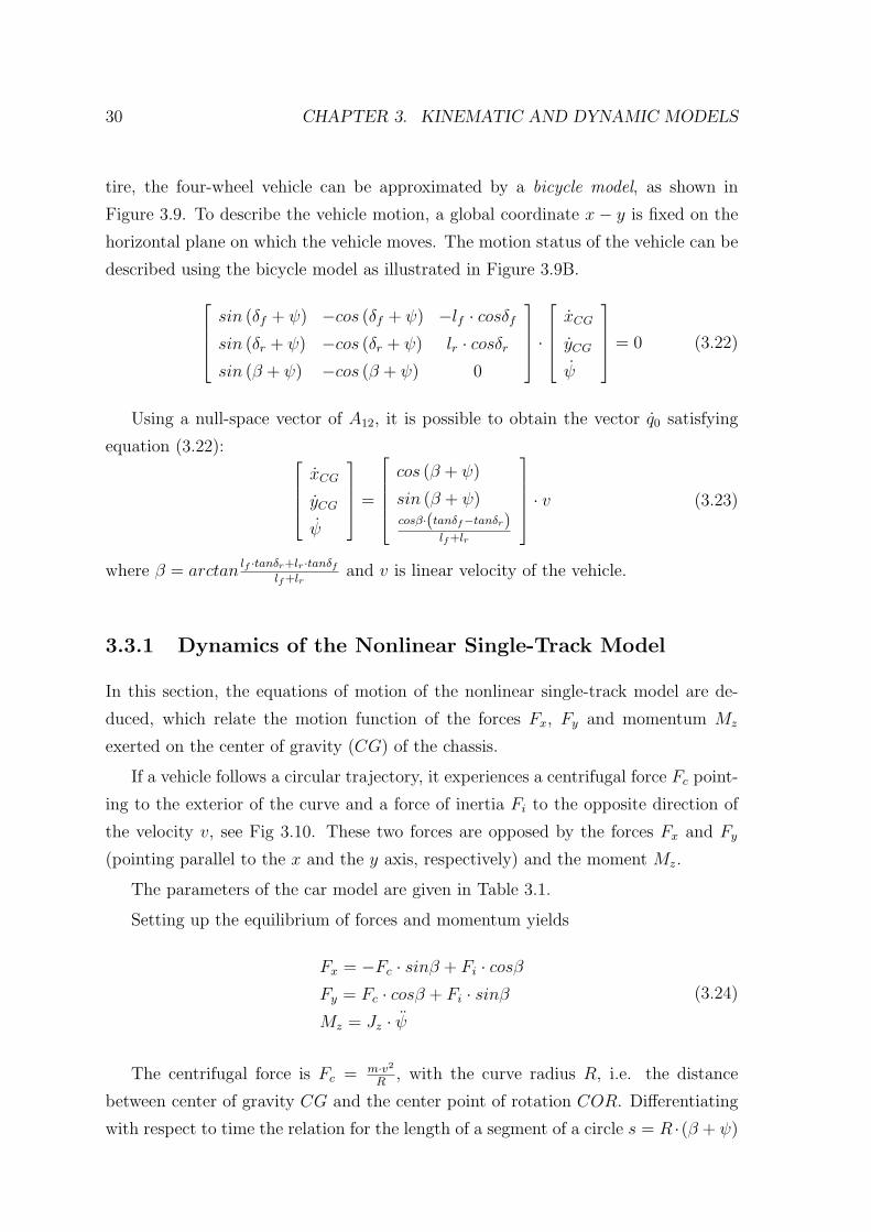
3.3.1 Dynamics of the Nonlinear Single-Track Model
In this section, the equations of motion of the nonlinear single-track model are de-
duced, which relate the motion function of the forces Fx, Fy and momentum Mz
exerted on the center of gravity (CG) of the chassis.
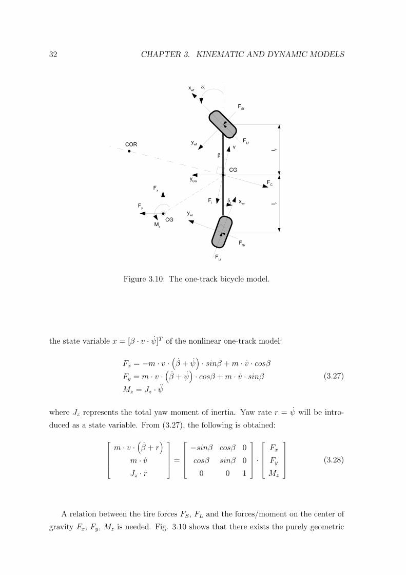
If a vehicle follows a circular trajectory, it experiences a centrifugal force Fc point-
ing to the exterior of the curve and a force of inertia Fi to the opposite direction of
the velocity v, see Fig 3.10. These two forces are opposed by the forces Fx and Fy
(pointing parallel to the x and the y axis, respectively) and the moment Mz.
The parameters of the car model are given in Table 3.1.
Setting up the equilibrium of forces and momentum yields
Fx = −Fc · sinβ + Fi · cosβ
Fy = Fc · cosβ + Fi · sinβ
Mz = Jz · ψ
(3.24)
The centrifugal force is Fc = m·v2
R, with the curve radius R, i.e. the distance
between center of gravity CG and the center point of rotation COR. Differentiating
with respect to time the relation for the length of a segment of a circle s = R ·(β + ψ)
3.3. KINEMATIC AND DYNAMIC MODELING FOR CAR-LIKE VEHICLE 31
Table 3.1: Parameters of the car modelParameter RemarksxCG, yCG Axis for the center of gravity co-ordinate systemxw, yw Axis for the wheel co-ordinate systemFLf , FLr Longitudinal forces of front and rear tires, respectivelyFSf , FSr Lateral forces of front and rear tires, respectivelyFx, Fy, Mz Forces and momentum on the center of gravity (CG)
of the chassisFc Centrifugal force of the vehicleFi Vehicle inertial forceFad Aerodynamic drag forceCad Aerodynamic drag coefficientAad Maximum vehicle cross-sectional areaρad Air densityv Longitudinal speed at the CG of the vehiclem Mass of the vehicleJz Inertia moment around center of gravity (CG)lf , lr Distance from front and rear tires to CG, respectivelyαf , αr Slip angle of front and rear tires, respectivelyδf , δr Wheel steering angle of front and rear tires, respectivelyβ Vehicle body sideslip angle (angle between xCG and v,
the vehicle velocityβf , βr Sideslip angle of front and rear chassisψ Yaw angler Yaw ratecf , cr Tire stiffness in the direction of yw and xw
µ Road friction coefficientR Curve radius - distance between center of gravity CG and
the center point of rotation COR
yields v = R ·(
β + ψ)
; (β + ψ) is the angle between the velocity v and the space-
fixed coordinate system (x0, y0). With this the centrifugal force depending on the
state variables is obtained as
Fc = m · v ·(
β + ψ)
(3.25)
In (3.24), Fi is the vehicle inertial force
Fi = m · v (3.26)
Inserting (3.25) and (3.26) in (3.24) yields the equations of motion depending on
32 CHAPTER 3. KINEMATIC AND DYNAMIC MODELS
Figure 3.10: The one-track bicycle model.
the state variable x = [β · v · ψ]T of the nonlinear one-track model:
Fx = −m · v ·(
β + ψ)
· sinβ +m · v · cosβ
Fy = m · v ·(
β + ψ)
· cosβ +m · v · sinβ
Mz = Jz · ψ
(3.27)
where Jz represents the total yaw moment of inertia. Yaw rate r = ψ will be intro-
duced as a state variable. From (3.27), the following is obtained:
m · v ·(
β + r)
m · v
Jz · r
=
−sinβ cosβ 0
cosβ sinβ 0
0 0 1
·
Fx
Fy
Mz
(3.28)
A relation between the tire forces FS, FL and the forces/moment on the center of
gravity Fx, Fy, Mz is needed. Fig. 3.10 shows that there exists the purely geometric
3.3. KINEMATIC AND DYNAMIC MODELING FOR CAR-LIKE VEHICLE 33
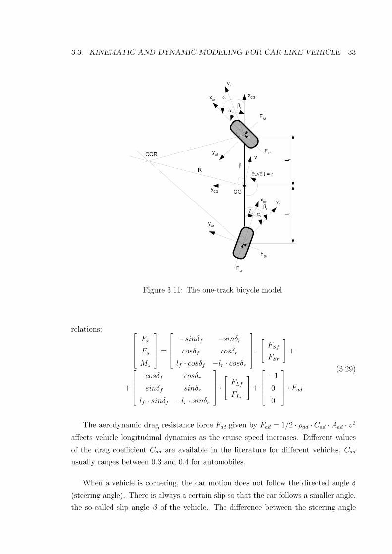
Figure 3.11: The one-track bicycle model.
relations:
Fx
Fy
Mz
=
−sinδf −sinδr
cosδf cosδr
lf · cosδf −lr · cosδr
·
FSf
FSr
+
+
cosδf cosδr
sinδf sinδr
lf · sinδf −lr · sinδr
·
FLf
FLr
+
−1
0
0
· Fad
(3.29)
The aerodynamic drag resistance force Fad given by Fad = 1/2 · ρad · Cad ·Aad · v2
affects vehicle longitudinal dynamics as the cruise speed increases. Different values
of the drag coefficient Cad are available in the literature for different vehicles, Cad
usually ranges between 0.3 and 0.4 for automobiles.
When a vehicle is cornering, the car motion does not follow the directed angle δ
(steering angle). There is always a certain slip so that the car follows a smaller angle,
the so-called slip angle β of the vehicle. The difference between the steering angle
34 CHAPTER 3. KINEMATIC AND DYNAMIC MODELS
and the slip angle of the vehicle is the slip angle α of the tire (see Fig. 3.11):
αf = δf − βf
αr = δr − βr
(3.30)
The front and rear chassis sideslip angles βf and βr are calculated by a “kinematic
model” from the state variables β, r and v
vf · sinβf = v · sinβ + lf · r
vr · sinβr = v · sinβ − lr · r(3.31)
The longitudinal components of these vectors must be equal, as they are connected
through the rigid chassis of the vehicle:
vf · cosβf = vr · cosβr = v · cosβ (3.32)
Eliminating vf and vr from (3.32) by using (3.31) leads to
tanβf = tanβ +lf ·r
v·cosβ
tanβr = tanβ − lr·rv·cosβ
(3.33)
The relationship between the tire sideslip angles and the tire side forces are given
by a nonlinear tire model
Fsf = Fsf (αf )
Fsr = Fsr(αr)(3.34)
A nonlinear tire model can be found in [70].
3.3.2 Linearized Single-Track Model
In the following a short overview of the assumptions has been is made to obtain the
linear model:
• vehicle sideslip angle β is small (β is limited to a value which is less than 10)
and the vehicle travels at constant speed, i.e. sinβ ≈ β, cosβ ≈ 1 and v = 0
(⇒ Fx = 0, ⇒ Fl is constantly zero). Then (3.28) becomes
m · v ·(
β + r)
Jz · r
=
Fy
Mz
(3.35)
3.3. KINEMATIC AND DYNAMIC MODELING FOR CAR-LIKE VEHICLE 35
• the steering angles δf and δr are small, i.e. sinδ ≈ δ and cosδ ≈ 1. Then (3.29)
becomes
Fy
Mz
=
1 1
lf −lr
·
Fsf (αf )
Fsr(αr)
(3.36)
• the front and rear chassis sideslip angles βf and βr are small. Then, from (3.33)
βf = β +lf ·r
v
βr = β − lr·rv
(3.37)
• the nonlinear tire characteristics can be approximated by
Fsf (αf ) = c∗f · αf = cf · µ · αf
Fsr(αr) = c∗r · αr = cr · µ · αr
(3.38)
where c∗f and c∗r are referred to as “cornering stiffnesses” in the automotive
literature.
From these assumptions, the linearized model has the following form:
m · v ·(
β + r)
Jz · r
=
1 1
lf −lr
·
cf · µ ·(
δf − β −lf ·r
v
)
cr · µ ·(
δr − β + lr·rv
)
(3.39)
Rearranging terms, the following linear state-space representation is obtained:
β
r
=
a11 a12
a21 a22
·
β
r
+
b11 b12
b21 b22
·
δf
δr
(3.40)
with
a11 = −µ·(cr+cf)
m·v
a12 =µ·(cr·lr−cf ·lf)
m·v2 − 1
a21 =µ·(cr·lr−cf ·lf)
Jz
a22 = −µ·(cr·l2r+cf ·l
2f)
Jz ·v
(3.41)
b11 =µ·cf
m·v
b21 = µ·cr
m·v
b21 =µ·cf ·lf
Jz
b21 = −µ·cr·lrJz
(3.42)
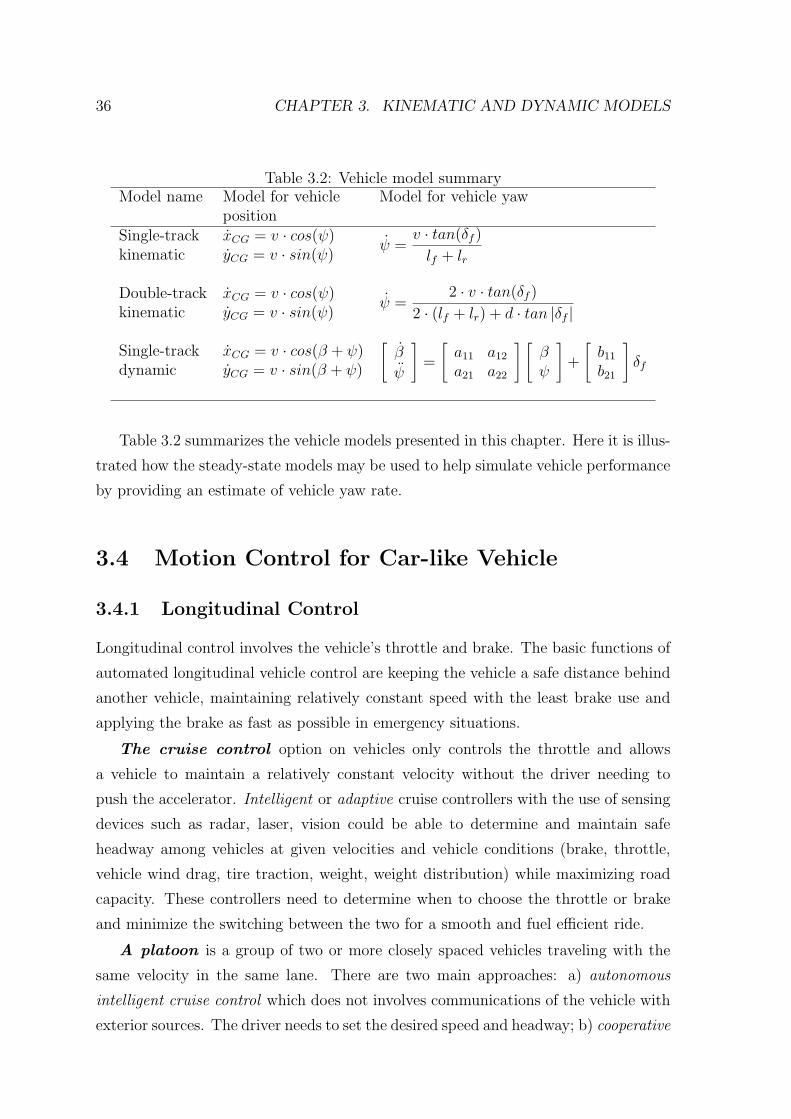
36 CHAPTER 3. KINEMATIC AND DYNAMIC MODELS
Table 3.2: Vehicle model summaryModel name Model for vehicle Model for vehicle yaw
positionSingle-track xCG = v · cos(ψ)
ψ =v · tan(δf )
lf + lrkinematic yCG = v · sin(ψ)
Double-track xCG = v · cos(ψ)ψ =
2 · v · tan(δf )
2 · (lf + lr) + d · tan |δf |kinematic yCG = v · sin(ψ)
Single-track xCG = v · cos(β + ψ)[
β
ψ
]
=
[
a11 a12
a21 a22
] [
βψ
]
+
[
b11b21
]
δfdynamic yCG = v · sin(β + ψ)
Table 3.2 summarizes the vehicle models presented in this chapter. Here it is illus-
trated how the steady-state models may be used to help simulate vehicle performance
by providing an estimate of vehicle yaw rate.
3.4 Motion Control for Car-like Vehicle
3.4.1 Longitudinal Control
Longitudinal control involves the vehicle’s throttle and brake. The basic functions of
automated longitudinal vehicle control are keeping the vehicle a safe distance behind
another vehicle, maintaining relatively constant speed with the least brake use and
applying the brake as fast as possible in emergency situations.
The cruise control option on vehicles only controls the throttle and allows
a vehicle to maintain a relatively constant velocity without the driver needing to
push the accelerator. Intelligent or adaptive cruise controllers with the use of sensing
devices such as radar, laser, vision could be able to determine and maintain safe
headway among vehicles at given velocities and vehicle conditions (brake, throttle,
vehicle wind drag, tire traction, weight, weight distribution) while maximizing road
capacity. These controllers need to determine when to choose the throttle or brake
and minimize the switching between the two for a smooth and fuel efficient ride.
A platoon is a group of two or more closely spaced vehicles traveling with the
same velocity in the same lane. There are two main approaches: a) autonomous
intelligent cruise control which does not involves communications of the vehicle with
exterior sources. The driver needs to set the desired speed and headway; b) cooperative
3.4. MOTION CONTROL FOR CAR-LIKE VEHICLE 37
intelligent cruise control allows the vehicle to communicate with the other vehicles
in its platoon.
3.4.2 Lateral Control
Lateral vehicle control ([71], [72], [73]) involves the steering of the vehicle. It is
concerned with lane keeping, turning, lane changing and avoiding objects that might
appear in front of the vehicle. There are two main approaches for automated steering:
a) look-down systems and b) look-ahead systems.
Look-down systems ([74], [75], [76]) follow wires or magnets embedded in the
middle of the lane. The major advantage of using a look-down system is that it is
unaffected by blinding conditions such as heavy precipitation, snow, fog or dust.
Look-ahead systems ([77], [78]) use cameras for lane following, radar for following
the preceding vehicle and lasers and/or cameras for lane switching.
3.4.3 Integration of Lateral and Longitudinal Controls
Lateral and longitudinal controllers ([79], [80]) need to be combined to determine the
brake pressure to keep the vehicle in its lane at the proper turning angle and losing
the least amount of speed. Another problem is obstacle avoidance when the controller
needs to determine if the vehicle should stop, go over or avoid an object in front of it.
If the vehicle avoids an obstacle, the controller need to determine the correct brake
pressure and turning movement to prevent the vehicle’s tires from losing contact with
the road.
38 CHAPTER 3. KINEMATIC AND DYNAMIC MODELS
Chapter 4
Path Planning
4.1 Introduction
Mobile robot research has made considerable advances in the past three decades.
Earlier works on mobile robots concentrated on path planning, where the objective
was to plan a collision free path and avoid stationary obstacles, while working in
an indoor/outdoor environment. Stationary obstacles are defined as fixed or non
moving obstructions such as walls or furniture. The most popular method in early
path planning was the configuration space method, where the mobile robot is shrunk
to a point, while corresponding growing the obstacles in order to compensate for
taking the robot as a point [98].
The many methods of path planning can be divided into three main categories:
roadmap approach [99], cell decomposition [100], and potential field [101] methods.
The roadmap approach is where the obstacle free area is modelled as a network of
lines. This network is then searched for a path that connects the start and goal
points. Cell decomposition is where the obstacle free area is subdivided into cells
that are interconnected to each other. These cells are then searched to find a path
that connects the start and goal points. Potential field methods use imaginary forces
acting on a robot. The goal position attracts the robot by pulling it towards the goal,
whereas the obstacles repulse the robot by pushing it away.
A trajectory is a path which is an explicit function of time. To have smooth
movement, the trajectory must be twice differentiable to give a continuous velocity
and acceleration. As a result, curve fitting is an integral part of trajectory planning.
There are a number of techniques used in curve fitting, including the use of B-splines,
cubic splines [102], clothoids, etc [103]. Simple path planning techniques assume that
39
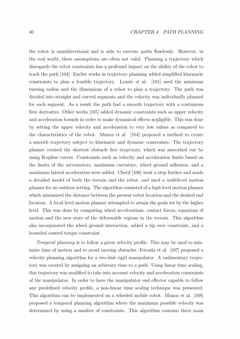
40 CHAPTER 4. PATH PLANNING
the robot is omnidirectional and is able to execute paths flawlessly. However, in
the real world, these assumptions are often not valid. Planning a trajectory which
disregards the robot constraints has a profound impact on the ability of the robot to
track the path [104]. Earlier works in trajectory planning added simplified kinematic
constraints to plan a feasible trajectory. Louste et al. [101] used the minimum
turning radius and the dimensions of a robot to plan a trajectory. The path was
divided into straight and curved segments and the velocity was individually planned
for each segment. As a result the path had a smooth trajectory with a continuous
first derivative. Other works [105] added dynamic constraints such as upper velocity
and acceleration bounds in order to make dynamical effects negligible. This was done
by setting the upper velocity and acceleration to very low values as compared to
the characteristics of the robot. Munoz et al. [104] proposed a method to create
a smooth trajectory subject to kinematic and dynamic constraints. The trajectory
planner created the shortest obstacle free trajectory, which was smoothed out by
using B-spline curves. Constraints such as velocity and acceleration limits based on
the limits of the servomotors, maximum curvature, wheel ground adhesion, and a
maximum lateral acceleration were added. Cherif [106] went a step further and made
a detailed model of both the terrain and the robot, and used a multilevel motion
planner for an outdoor setting. The algorithm consisted of a high level motion planner
which minimized the distance between the present robot location and the desired end
location. A local level motion planner attempted to attain the goals set by the higher
level. This was done by computing wheel accelerations, contact forces, equations of
motion and the new state of the deformable regions in the terrain. This algorithm
also incorporated the wheel ground interaction, added a tip over constraint, and a
bounded control torque constraint.
Temporal planning is to follow a given velocity profile. This may be used to min-
imize time of motion and to avoid moving obstacles. Fotouhi et al. [107] proposed a
velocity planning algorithm for a two-link rigid manipulator. A rudimentary trajec-
tory was created by assigning an arbitrary time to a path. Using linear time scaling,
this trajectory was modified to take into account velocity and acceleration constraints
of the manipulator. In order to have the manipulator end effector capable to follow
any predefined velocity profile, a non-linear time scaling technique was presented.
This algorithm can be implemented on a wheeled mobile robot. Munoz et al. [108]
proposed a temporal planning algorithm where the maximum possible velocity was
determined by using a number of constraints. This algorithm contains three main
4.2. QUINTIC EQUATIONS 41
parts. The first was the temporal planning process, where the maximum possible
velocity was determined using the following constraints: velocity, acceleration, wheel
slippage, moments, and a built-in safety speed. The next step was to create a smooth
path using B-splines while avoiding moving obstacles. The final step was to merge
the maximum velocity with the path, thereby creating a trajectory. While most other
works use constant upper velocity, acceleration, and deceleration bounds, Prado et
al. [109] created upper bound velocity, acceleration and deceleration functions which
changed with the path. In a more recent work, Prado et al. [110] introduced a ve-
locity profiling technique that divides the path into smaller segments. The velocity
profile of each segment is generated by a cubic polynomial which is then integrated to
obtain position and differentiated to obtain the acceleration. The profile is checked
with a number of constraints and is iteratively modified until the constraints are fully
satisfied. He also provided a method to avoid moving obstacles by modifying the
velocity profile of the mobile robot. If a moving obstacle was encountered, the robot
speed was reduced until the obstacle had cleared the path.
4.2 Quintic Equations
Let P (u) = p1(u), p2(u), ..., pn(u), u ∈ [0, 1] be a route defined by a set of points
computed by a path planner as shown in Figure 4.1. Each point pi is composed of
three basic elements: xi, yi and φi where i = 1, 2, ..., n. The first two components,
define position relative to a global reference frame shown in Figure 4.1. The last
component, φi, is the heading (orientation) from one point to the next defined in the
X−Y plane. There are several methods to join these points with a curve. The easiest
method is to connect the points with straight lines; however, there are sudden changes
in slope which in mobile robotics means a discontinuous velocity. Another method
could be to use a high order polynomial. However, if there are numerous points,
the path may become wavy due to the oscillatory nature of high order polynomials.
A more effective method is the use of piecewise quintic polynomials, also known as
quintic splines. These quintic splines are ideal since they provide a continuity in
position, heading, curvature, velocity, and acceleration [111], [112].
42 CHAPTER 4. PATH PLANNING
0 10 20 30 40 50 600
10
20
30
40
50
60
p1(3,7,0) p
2(20,7,0)
p3(22,9,pi/2)
p4(22,18,pi/2)
p5(24,20,0)
p6(38,20,0)
p7(40,22,pi/2)
p8(40,31,pi/2)
p9(42,34,pi/8)
p10
(47,42,pi/2)
p11
(38,51,pi)
p12
(30,46,−3*pi/4)
p13
(27,44,pi)
p14
(0,44,pi)
Figure 4.1: Path planning example using quintic polynomial curves.
Closed-form expressions of the quintic G2-splines can be presented as follows
pi,i+1(u) =
xi,i+1(u)
yi,i+1(u)
φi,i+1(u)
=
αi0 + αi1u+ αi2u2 + αi3u
3 + αi4u4 + αi5u
5
βi0 + βi1u+ βi2u2 + βi3u
3 + βi4u4 + βi5u
5
φi(u)
(4.1)
where
αi0 = xi(0)
αi1 = η1 · cos(φi(0))
αi2 = 12(η3 · cos(φi(0))− η2
1 · ki · sin(φi(0)))
αi3 = 10 · (xi+1(0)− xi(0))−(
6 · η1 + 32· η3
)
· cos(φi(0))−
−(
4 · η2 −12· η4
)
· cos(φi+1(0)) + 32· η2
1 · ki · sin(φi(0))− 12· η2
2 · ki+1 · sin(φi+1(0))
αi4 = −15 · (xi+1(0)− xi(0)) +(
8 · η1 + 32· η3
)
· cos(φi(0))+
+ (7 · η2 − η4) · cos(φi+1(0))− 32· η2
1 · ki · sin(φi(0)) + η22 · ki+1 · sin(φi+1(0))
αi5 = 6 · (xi+1(0)− xi(0))−(
3 · η1 + 12· η3
)
· cos(φi(0))−
−(
3 · η2 −12η4
)
· cos(φi+1(0)) + 12· η2
1 · ki · sin(φi(0))− 12η2
2 · ki+1 · sin(φi+1(0))
4.3. VELOCITY PLANNING 43
βi0 = yi(0)
βi1 = η1 · cos(φi(0))
βi2 = 12(η3 · cos(φi(0)) + η2
1 · ki · sin(φi(0)))
βi3 = 10 · (yi+1(0)− yi(0))−(
6 · η1 + 32· η3
)
· sin(φi(0))−
−(
4 · η2 −12· η4
)
· sin(φi+1(0))− 32· η2
1 · ki · cos(φi(0)) + 12· η2
2 · ki+1 · cos(φi+1(0))
βi4 = −15 · (yi+1(0)− yi(0)) +(
8 · η1 + 32· η3
)
· sin(φi(0))+
+ (7 · η2 − η4) · sin(φi+1(0)) + 32· η2
1 · ki · cos(φi(0))− η22 · ki+1 · cos(φi+1(0))
βi5 = 6 · (yi+1(0)− yi(0))−(
3 · η1 + 12· η3
)
· sin(φi(0))−
−(
3 · η2 −12η4
)
· sin(φi+1(0))− 12· η2
1 · ki · cos(φi(0)) + 12η2
2 · ki+1 · cos(φi+1(0))
Where ki and ki+1 are scalar curvatures, ki ∈ ℜ, i = 1, 2, ..., n and can be arbitrary
assigned (in this case ki = 0). The real parameters ηm, m = 1, 2, 3, 4, appearing
in above expressions can be packed together to form the four-dimensional vector
η := [η1, η2, η3, η4]T ∈ H := ℜ+×ℜ+×ℜ×ℜ. η1 mainly influences the shape of the
curve at the beginning, η2 affects its closing. In practice, to attain symmetric curves
we have imposed η1 = η2. In Figure 4.2, η1 and η2 are varied whereas η3 and η4 are
constant (η3 = η4 = 0). Parameters η3 and η4 modulate the curvature variation at the
beginning and at the closing of the spline respectively. In Figure 4.3, η1 and η2 are
kept constant and curves are traced for different values of η3 and η4. Very negative
values of η3 (very positive value for η4) cause strong curvature variations.
According to the theory of planar curves, an explicit expression of curvature,
ki,i+1(u) is
ki,i+1(u) =xi,i+1(u) · yi,i+1(u)− xi,i+1(u) · yi,i+1(u)
(
x2i,i+1(u) + y2
i,i+1(u))3/2
(4.2)
The function ki,i+1(u) is continuous over [0, 1] because pi,i+1(u) is a G2-curve.
The curve length measured along two points pi, pi+1 is denoted by si,i+1(u); it can
be expressed as
si,i+1(u) =∫ u
u0
√
x2i,i+1(u) + y2
i,i+1(u) · du (4.3)
and we denote by s−1i,i+1 : [0, si,i+1(u1)] → [u0u1] its inverse function that is evidently
a continuous function.
4.3 Velocity Planning
The aim of this section is to obtain a longitudinal and angular velocity profiles (v(t)
and ω(t)). The profile must be compatible with the assigned total path length sk and
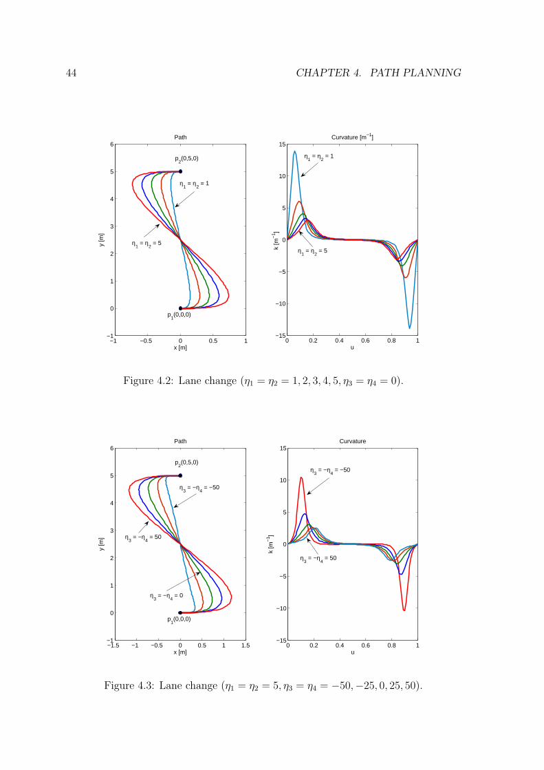
44 CHAPTER 4. PATH PLANNING
−1 −0.5 0 0.5 1−1
0
1
2
3
4
5
6
x [m]
y [m
]
Path
p1(0,0,0)
p2(0,5,0)
η1 = η
2 = 1
η1 = η
2 = 5
0 0.2 0.4 0.6 0.8 1−15
−10
−5
0
5
10
15
u
k [m
−1 ]
Curvature [m−1]
η1 = η
2 = 1
η1 = η
2 = 5
Figure 4.2: Lane change (η1 = η2 = 1, 2, 3, 4, 5, η3 = η4 = 0).
−1.5 −1 −0.5 0 0.5 1 1.5−1
0
1
2
3
4
5
6Path
x [m]
y [m
]
p1(0,0,0)
p2(0,5,0)
η3 = −η
4 = −50
η3 = −η
4 = 50
η3 = −η
4 = 0
0 0.2 0.4 0.6 0.8 1−15
−10
−5
0
5
10
15Curvature
u
k [m
−1 ]
η3 = −η
4 = −50
η3 = −η
4 = 50
Figure 4.3: Lane change (η1 = η2 = 5, η3 = η4 = −50,−25, 0, 25, 50).
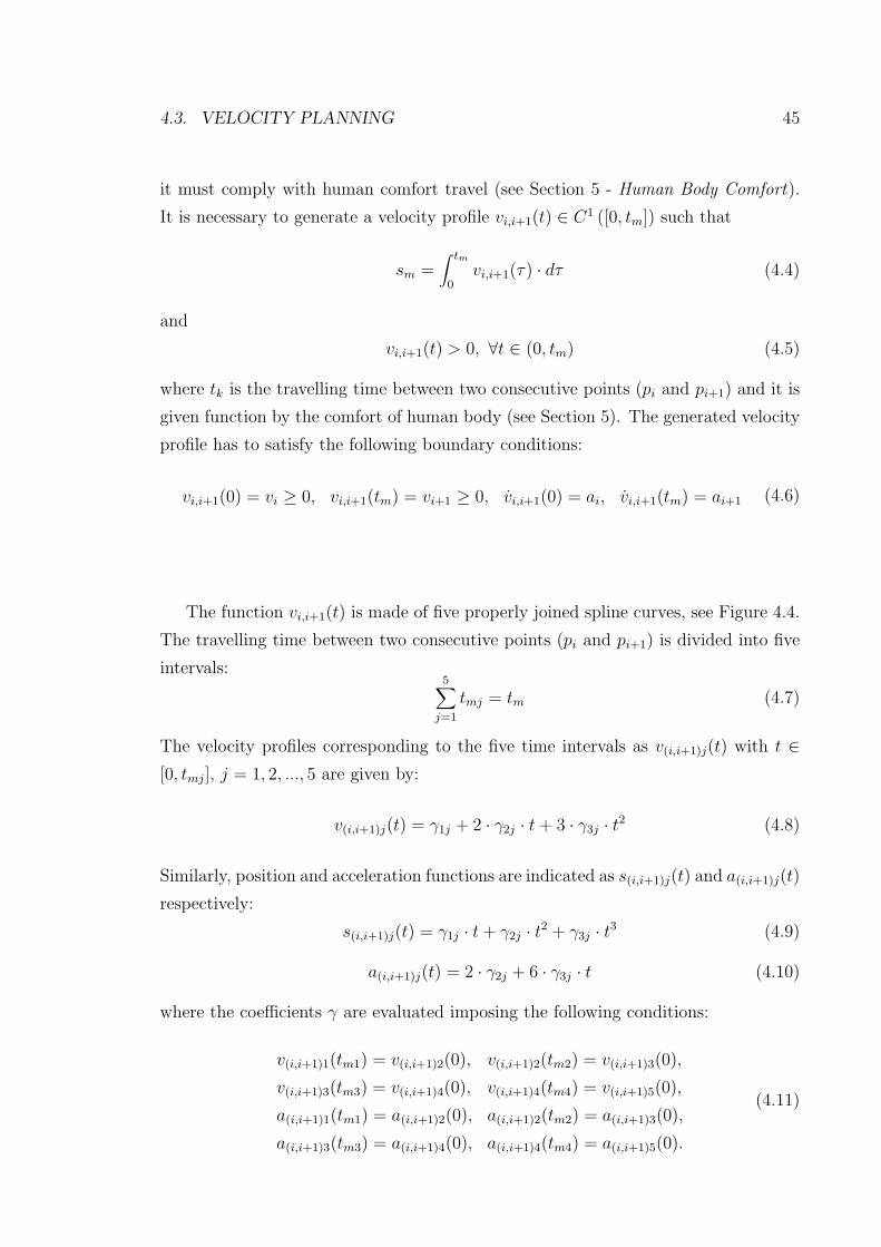
4.3. VELOCITY PLANNING 45
it must comply with human comfort travel (see Section 5 - Human Body Comfort).
It is necessary to generate a velocity profile vi,i+1(t) ∈ C1 ([0, tm]) such that
sm =∫ tm
0vi,i+1(τ) · dτ (4.4)
and
vi,i+1(t) > 0, ∀t ∈ (0, tm) (4.5)
where tk is the travelling time between two consecutive points (pi and pi+1) and it is
given function by the comfort of human body (see Section 5). The generated velocity
profile has to satisfy the following boundary conditions:
vi,i+1(0) = vi ≥ 0, vi,i+1(tm) = vi+1 ≥ 0, vi,i+1(0) = ai, vi,i+1(tm) = ai+1 (4.6)
The function vi,i+1(t) is made of five properly joined spline curves, see Figure 4.4.
The travelling time between two consecutive points (pi and pi+1) is divided into five
intervals:5∑
j=1
tmj = tm (4.7)
The velocity profiles corresponding to the five time intervals as v(i,i+1)j(t) with t ∈
[0, tmj], j = 1, 2, ..., 5 are given by:
v(i,i+1)j(t) = γ1j + 2 · γ2j · t+ 3 · γ3j · t2 (4.8)
Similarly, position and acceleration functions are indicated as s(i,i+1)j(t) and a(i,i+1)j(t)
respectively:
s(i,i+1)j(t) = γ1j · t+ γ2j · t2 + γ3j · t
3 (4.9)
a(i,i+1)j(t) = 2 · γ2j + 6 · γ3j · t (4.10)
where the coefficients γ are evaluated imposing the following conditions:
v(i,i+1)1(tm1) = v(i,i+1)2(0), v(i,i+1)2(tm2) = v(i,i+1)3(0),
v(i,i+1)3(tm3) = v(i,i+1)4(0), v(i,i+1)4(tm4) = v(i,i+1)5(0),
a(i,i+1)1(tm1) = a(i,i+1)2(0), a(i,i+1)2(tm2) = a(i,i+1)3(0),
a(i,i+1)3(tm3) = a(i,i+1)4(0), a(i,i+1)4(tm4) = a(i,i+1)5(0).
(4.11)
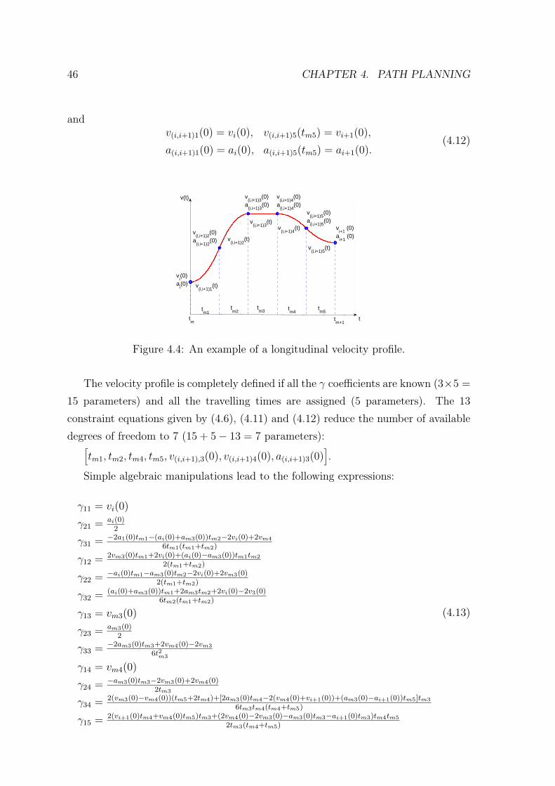
46 CHAPTER 4. PATH PLANNING
andv(i,i+1)1(0) = vi(0), v(i,i+1)5(tm5) = vi+1(0),
a(i,i+1)1(0) = ai(0), a(i,i+1)5(tm5) = ai+1(0).(4.12)
v(i,i+1)2
(t)
v(i,i+1)3
(t) v
(i,i+1)4(t)
v(i,i+1)5
(t)
v(i,i+1)2
(0) a
(i,i+1)2(0)
v(i,i+1)3
(0) a
(i,i+1)3(0)
tm2
tm3
tm4
tm5
v(i,i+1)5
(0) a
(i,i+1)5(0)
v(i,i+1)4
(0) a
(i,i+1)4(0)
tm1
tm+1
vi(0)
ai(0)
vi+1
(0)a
i+1 (0)
v(i,i+1)1
(t)
tm
t
v(t)
Figure 4.4: An example of a longitudinal velocity profile.
The velocity profile is completely defined if all the γ coefficients are known (3×5 =
15 parameters) and all the travelling times are assigned (5 parameters). The 13
constraint equations given by (4.6), (4.11) and (4.12) reduce the number of available
degrees of freedom to 7 (15 + 5− 13 = 7 parameters):[
tm1, tm2, tm4, tm5, v(i,i+1),3(0), v(i,i+1)4(0), a(i,i+1)3(0)]
.
Simple algebraic manipulations lead to the following expressions:
γ11 = vi(0)
γ21 = ai(0)2
γ31 = −2a1(0)tm1−(ai(0)+am3(0))tm2−2vi(0)+2vm4
6tm1(tm1+tm2)
γ12 = 2vm3(0)tm1+2vi(0)+(ai(0)−am3(0))tm1tm2
2(tm1+tm2)
γ22 = −ai(0)tm1−am3(0)tm2−2vi(0)+2vm3(0)2(tm1+tm2)
γ32 = (ai(0)+am3(0))tm1+2am3tm2+2vi(0)−2v3(0)6tm2(tm1+tm2)
γ13 = vm3(0)
γ23 = am3(0)2
γ33 = −2am3(0)tm3+2vm4(0)−2vm3
6t2m3
γ14 = vm4(0)
γ24 = −am3(0)tm3−2vm3(0)+2vm4(0)2tm3
γ34 = 2(vm3(0)−vm4(0))(tm5+2tm4)+[2am3(0)tm4−2(vm4(0)+vi+1(0))+(am3(0)−ai+1(0))tm5]tm3
6tm3tm4(tm4+tm5)
γ15 = 2(vi+1(0)tm4+vm4(0)tm5)tm3+(2vm4(0)−2vm3(0)−am3(0)tm3−ai+1(0)tm3)tm4tm5
2tm3(tm4+tm5)
(4.13)
4.3. VELOCITY PLANNING 47
γ25 = 2(vm3(0)−vm4(0))tm4−(2vm4(0)−2vi+1(0)−am3(0)tm4+ai+1(0)tm5)tm3
2tm3(tm4+tm5)
γ35 = (2vm4(0)−2vi+1(0)−am3(0)tm4+ai+1(0)tm4+2ai+1(0)tm5)tm3−2(vm3(0)−vm4(0))tm4
6tm3tm5(tm4+tm5)
(4.14)
where m := (i, i+ 1)
To satisfy (4.7) it is necessary to further impose tm3 = tm−(tm1 + tm2 + tm4 + tm5)
where, necessarily, tm1 + tm2 + tm4 + tm5 < tm. Velocities vi(0), v(i,i+1)3(0), v(i,i+1))4(0)
and vi+1(0) can be freely assigned respecting constraints (4.6), and v(i,i+1)2(0),
v(i,i+1)5(0) are calculated by (4.8). In the same way ai(0), a(i,i+1)3(0) and ai+1(0)
are given respecting (4.6), and a(i,i+1)2(0), a(i,i+1)4(0), a(i,i+1)5(0) are calculated using
(4.10).
If we impose the following two further constraints:
a(i,i+1)3(0) = 0, a(i,i+1)3(tm3) = 0 (4.15)
the number of free parameters decreases to five:[
tm1, tm2, tm4, tm5, v(i,i+1)3(0)]
because
v(i,i+1)4(0) = v(i,i+1)3(0) and a(i,i+1)3(0) = 0. In this case, equations (4.13) become
γ11 = vi(0)
γ21 = ai(0)2
γ31 =−2a1(0)tm1−ai(0)tm2−2vi(0)+2v(i,i+1)4
6tm1(tm1+tm2)
γ12 =2v(i,i+1)3(0)tm1+2vi(0)+ai(0)tm1tm2
2(tm1+tm2)
γ22 =−ai(0)tm1−2vi(0)+2v(i,i+1)3(0)
2(tm1+tm2)
γ32 = ai(0)tm1+2vi(0)−2v3(0)6tm2(tm1+tm2)
γ13 = v(i,i+1)3(0)
γ23 = 0
γ33 = 0
γ14 = v(i,i+1)3(0)
γ24 = 0
γ34 =−2(v(i,i+1)3(0)−vi+1(0))−ai+1(0)tm5
6tm4(tm4+tm5)
γ15 =2(vi+1(0)tm4+v(i,i+1)4(0)tm5)−ai+1(0)tm4tm5
2(tm4+tm5)
γ25 =−(2v(i,i+1)3(0)−2vi+1(0)+ai+1(0)tm5)
2(tm4+tm5)
γ35 =2v(i,i+1)3(0)−2vi+1(0)+ai+1(0)tm4+2ai+1(0)tm5
6tm5(tm4+tm5)
(4.16)
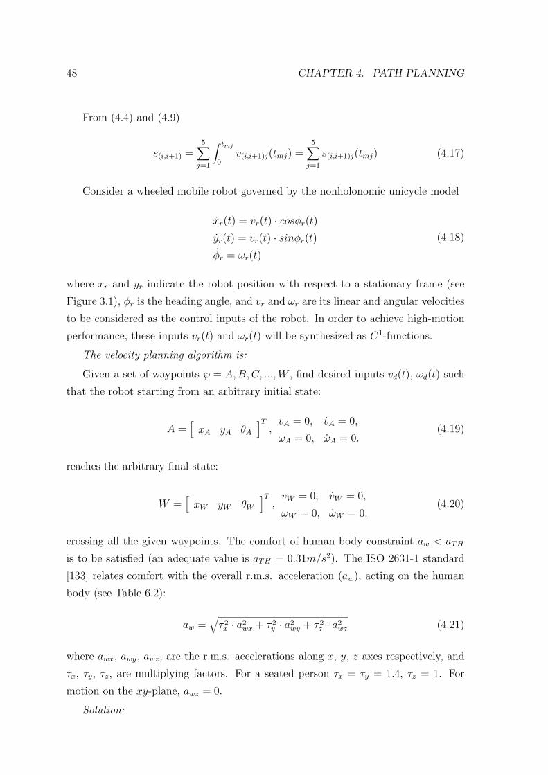
48 CHAPTER 4. PATH PLANNING
From (4.4) and (4.9)
s(i,i+1) =5∑
j=1
∫ tmj
0v(i,i+1)j(tmj) =
5∑
j=1
s(i,i+1)j(tmj) (4.17)
Consider a wheeled mobile robot governed by the nonholonomic unicycle model
xr(t) = vr(t) · cosφr(t)
yr(t) = vr(t) · sinφr(t)
φr = ωr(t)
(4.18)
where xr and yr indicate the robot position with respect to a stationary frame (see
Figure 3.1), φr is the heading angle, and vr and ωr are its linear and angular velocities
to be considered as the control inputs of the robot. In order to achieve high-motion
performance, these inputs vr(t) and ωr(t) will be synthesized as C1-functions.
The velocity planning algorithm is:
Given a set of waypoints ℘ = A,B,C, ...,W , find desired inputs vd(t), ωd(t) such
that the robot starting from an arbitrary initial state:
A =[
xA yA θA
]T,vA = 0, vA = 0,
ωA = 0, ωA = 0.(4.19)
reaches the arbitrary final state:
W =[
xW yW θW
]T,vW = 0, vW = 0,
ωW = 0, ωW = 0.(4.20)
crossing all the given waypoints. The comfort of human body constraint aw < aTH
is to be satisfied (an adequate value is aTH = 0.31m/s2). The ISO 2631-1 standard
[133] relates comfort with the overall r.m.s. acceleration (aw), acting on the human
body (see Table 6.2):
aw =√
τ 2x · a
2wx + τ 2
y · a2wy + τ 2
z · a2wz (4.21)
where awx, awy, awz, are the r.m.s. accelerations along x, y, z axes respectively, and
τx, τy, τz, are multiplying factors. For a seated person τx = τy = 1.4, τz = 1. For
motion on the xy-plane, awz = 0.
Solution:
4.3. VELOCITY PLANNING 49
1. Determine a path connecting A (start point) with W (final point) using
℘(i,i+1)(u) =
x(i,i+1)(u)
y(i,i+1)(u)
θ(i,i+1)(u)
=
αi0 + αi1u+ αi2u2 + αi3u
3 + ...
βi0 + βi1u+ βi2u2 + βi3u
3 + ...
θi(u)
(4.22)
where u ∈ [0, 1], αij and βij, with i = A,B,C, ..., j = 0, 1, ... are constants to be
found function of the type of the curve (e.g. cubic splines, trigonometric splines
or quintic splines). Next, calculate the curvature of each segment path
k(i,i+1)(u) = 1(
x2(i,i+1)
(u)+y2(i,i+1)
(u)
)3/2 ·
·(
x(i,i+1)(u) · y(i,i+1)(u)− x(i,i+1)(u) · y(i,i+1)(u))
(4.23)
and curve length
s(i,i+1)(u) =∫ 1
0
√
x2(i,i+1)(u) + y2
(i,i+1)(u) · du (4.24)
where i = A,B,C, ... and u ∈ [0, 1].
2. Determine a time t(i,i+1) and an average velocity v(i,i+1) for each segment (i, i+1)
of the path ℘. The time and the average velocity are calculate function of the
comfort of human body constraint:
t(i,i+1) =
√
√
√
√
2 · s(i,i+1)
awxy(i,i+1)
(4.25)
v(i,i+1) = awxy(i,i+1) · t(i,i+1). (4.26)
Accordingly (4.21) when aw = 0.315m/s2, the maximum value of awx or awy
must be less than 0.225m/s2 (see Fig. 4.5). The most restrictive case is when
the trajectory of the robot is an arc of a circle, with awxy = awx = awy. In this
case the accelerations should be under 0.16m/s2, i.e. awx = awy ≤ 0.16m/s2.
3. Calculate an initial linear velocity profile v(i,i+1)(t) with t ∈ [ti, ti+1]. Each
velocity profile is generated with five properly joined spline curves:
v(i,i+1)j(t) = γ1j + 2 · γ2j · t+ 3 · γ3j · t2 (4.27)
50 CHAPTER 4. PATH PLANNING
−0.4
−0.2
0
0.2
0.4
−0.4
−0.2
0
0.2
0.40
0.1
0.2
0.3
0.4
0.5
0.6
0.7
0.8
awx
awy
a w
aw = 0.315 m/s2
Figure 4.5: Restrictive cases of aw.
where i = A,B,C, ... and j = 1, 2..5. Next, calculate the curve length, s(i,i+1)(t),
and the acceleration profile, a(i,i+1)(t), using:
s(i,i+1)j(t) = γ1j · t+ γ2j · t2 + γ3j · t
3 (4.28)
a(i,i+1)j(t) = 2 · γ2j + 6 · γ3j · t (4.29)
where the coefficients γ are defined by (4.13).
4. Calculate angular velocity profile ω(i,i+1)(t) using Frenet formula
ω(i,i+1)(t) := v(i,i+1)(t) · k(i,i+1)(s(i,i+1))∣
∣
∣
∣s(i,i+1)=∫ t(i,i+1)0 v(i,i+1)(τ)·dτ
(4.30)
5. Calculate the overall r.m.s. acceleration aw(i,i+1) for each path segment using
equation (4.21).
6. IF aw(i,i+1) > aTH THEN increase the time interval for this path segment (a
good performance has been achieved using an increase of 10% in each iteration)
and GO TO step 3.
Consider the example depicted in Figure 4.1 where the larger circles represent
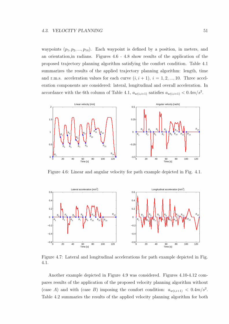
4.3. VELOCITY PLANNING 51
waypoints (p1, p2, ..., p14). Each waypoint is defined by a position, in meters, and
an orientation,in radians. Figures 4.6 - 4.8 show results of the application of the
proposed trajectory planning algorithm satisfying the comfort condition. Table 4.1
summarizes the results of the applied trajectory planning algorithm: length, time
and r.m.s. acceleration values for each curve (i, i + 1), i = 1, 2, ..., 10. Three accel-
eration components are considered: lateral, longitudinal and overall acceleration. In
accordance with the 6th column of Table 4.1, aw(i,i+1) satisfies aw(i,i+1) < 0.4m/s2.
0 20 40 60 80 100 1200
0.5
1
1.5
2 Linear velocity [m/s]
Time [s]
p14
p13
p12
p11
p10
p9
p8
p7
p6
p5
p4
p3
p2
p1
0 20 40 60 80 100 120−0.5
−0.25
0
0.25
0.5 Angular velocity [rad/s]
Time [s]
p14
p13
p12
p11
p10
p9
p8
p7
p6
p5
p4
p3
p2
p1
Figure 4.6: Linear and angular velocity for path example depicted in Fig. 4.1.
0 20 40 60 80 100 120−0.6
−0.4
−0.2
0
0.2
0.4
0.6Lateral acceleration [m/s2]
Time [s]
p14
p13
p12
p11
p10
p9
p8
p7
p6
p5
p4
p3
p2
p1
0 20 40 60 80 100 120−0.6
−0.4
−0.2
0
0.2
0.4
0.6 Longitudinal acceleration [m/s2]
Time [s]
p1
p2
p3
p4
p5
p6
p7
p8
p9
p10
p11
p12
p13
p14
Figure 4.7: Lateral and longitudinal accelerations for path example depicted in Fig.4.1.
Another example depicted in Figure 4.9 was considered. Figures 4.10-4.12 com-
pares results of the application of the proposed velocity planning algorithm without
(case A) and with (case B) imposing the comfort condition: aw(i,i+1) < 0.4m/s2.
Table 4.2 summaries the results of the applied velocity planning algorithm for both
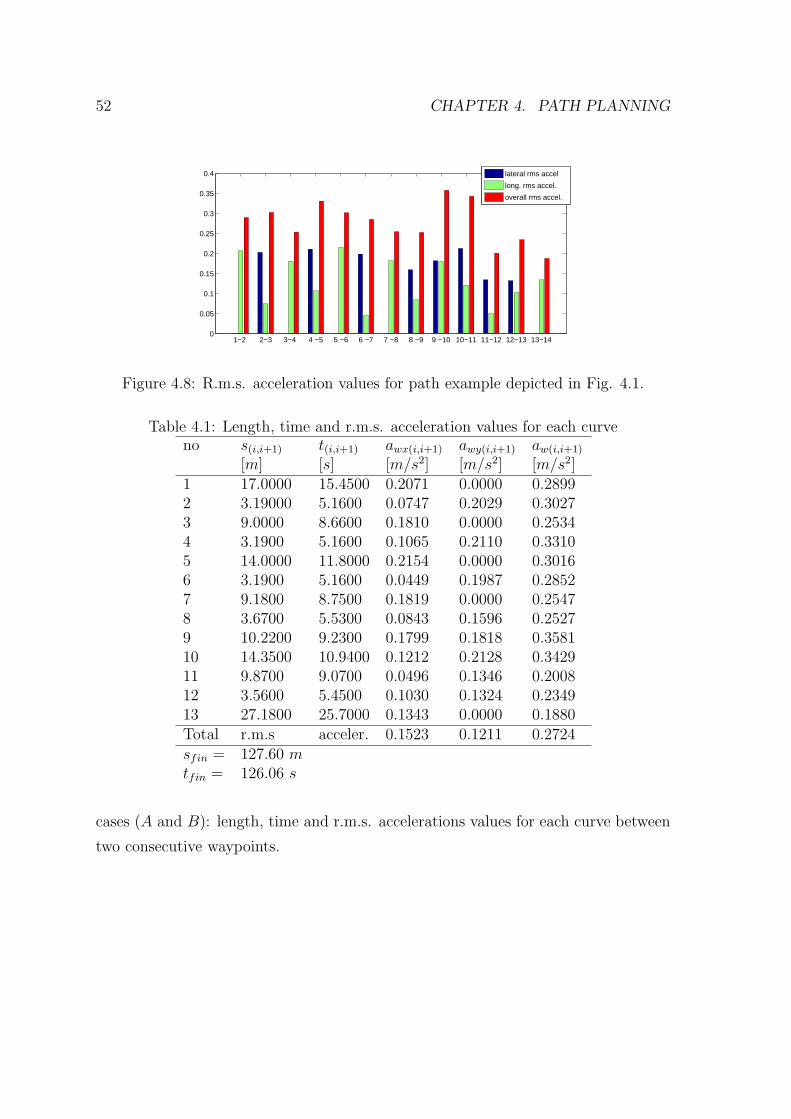
52 CHAPTER 4. PATH PLANNING
1−2 2−3 3−4 4 −5 5 −6 6 −7 7 −8 8 −9 9 −10 10−11 11−12 12−13 13−140
0.05
0.1
0.15
0.2
0.25
0.3
0.35
0.4
lateral rms accel
long. rms accel.
overall rms accel.
Figure 4.8: R.m.s. acceleration values for path example depicted in Fig. 4.1.
Table 4.1: Length, time and r.m.s. acceleration values for each curveno s(i,i+1) t(i,i+1) awx(i,i+1) awy(i,i+1) aw(i,i+1)
[m] [s] [m/s2] [m/s2] [m/s2]1 17.0000 15.4500 0.2071 0.0000 0.28992 3.19000 5.1600 0.0747 0.2029 0.30273 9.0000 8.6600 0.1810 0.0000 0.25344 3.1900 5.1600 0.1065 0.2110 0.33105 14.0000 11.8000 0.2154 0.0000 0.30166 3.1900 5.1600 0.0449 0.1987 0.28527 9.1800 8.7500 0.1819 0.0000 0.25478 3.6700 5.5300 0.0843 0.1596 0.25279 10.2200 9.2300 0.1799 0.1818 0.358110 14.3500 10.9400 0.1212 0.2128 0.342911 9.8700 9.0700 0.0496 0.1346 0.200812 3.5600 5.4500 0.1030 0.1324 0.234913 27.1800 25.7000 0.1343 0.0000 0.1880Total r.m.s acceler. 0.1523 0.1211 0.2724sfin = 127.60 mtfin = 126.06 s
cases (A and B): length, time and r.m.s. accelerations values for each curve between
two consecutive waypoints.
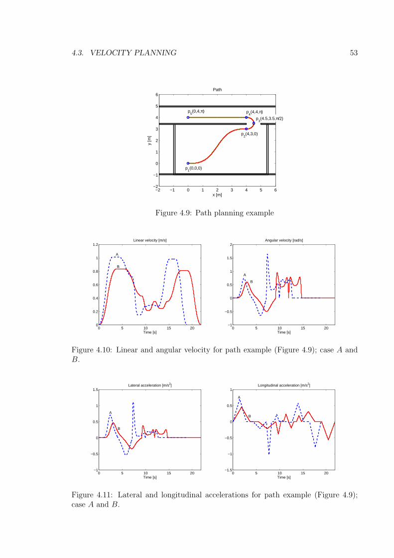
4.3. VELOCITY PLANNING 53
−2 −1 0 1 2 3 4 5 6−2
−1
0
1
2
3
4
5
6Path
x [m]
y [m
]
p1(0,0,0)
p2(4,3,0)
p3(4.5,3.5,π/2)
p4(4,4,π)p
5(0,4,π)
Figure 4.9: Path planning example
0 5 10 15 200
0.2
0.4
0.6
0.8
1
1.2Linear velocity [m/s]
Time [s]
A
B
0 5 10 15 20−1
−0.5
0
0.5
1
1.5
2Angular velocity [rad/s]
Time [s]
A
B
Figure 4.10: Linear and angular velocity for path example (Figure 4.9); case A andB.
0 5 10 15 20−1
−0.5
0
0.5
1
1.5Lateral acceleration [m/s2]
Time [s]
A
B
0 5 10 15 20−1.5
−1
−0.5
0
0.5
1Longitudinal acceleration [m/s2]
Time [s]
A
B
Figure 4.11: Lateral and longitudinal accelerations for path example (Figure 4.9);case A and B.
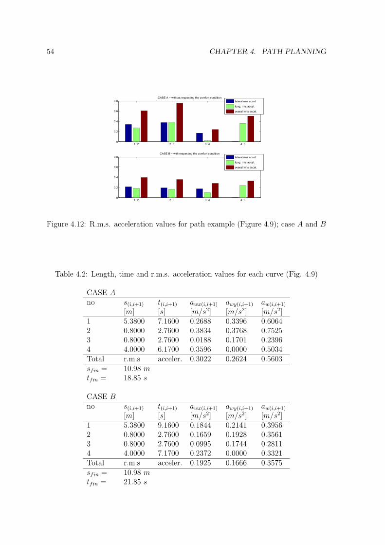
54 CHAPTER 4. PATH PLANNING
1−2 2−3 3−4 4−50
0.2
0.4
0.6
0.8CASE A − without respecting the comfort condition
1−2 2−3 3−4 4−50
0.2
0.4
0.6
0.8CASE B − with respecting the comfort condition
lateral rms accel
long. rms accel.
overall rms accel.
lateral rms accel
long. rms accel.
overall rms accel.
Figure 4.12: R.m.s. acceleration values for path example (Figure 4.9); case A and B
Table 4.2: Length, time and r.m.s. acceleration values for each curve (Fig. 4.9)
CASE Ano s(i,i+1) t(i,i+1) awx(i,i+1) awy(i,i+1) aw(i,i+1)
[m] [s] [m/s2] [m/s2] [m/s2]1 5.3800 7.1600 0.2688 0.3396 0.60642 0.8000 2.7600 0.3834 0.3768 0.75253 0.8000 2.7600 0.0188 0.1701 0.23964 4.0000 6.1700 0.3596 0.0000 0.5034Total r.m.s acceler. 0.3022 0.2624 0.5603sfin = 10.98 mtfin = 18.85 s
CASE Bno s(i,i+1) t(i,i+1) awx(i,i+1) awy(i,i+1) aw(i,i+1)
[m] [s] [m/s2] [m/s2] [m/s2]1 5.3800 9.1600 0.1844 0.2141 0.39562 0.8000 2.7600 0.1659 0.1928 0.35613 0.8000 2.7600 0.0995 0.1744 0.28114 4.0000 7.1700 0.2372 0.0000 0.3321Total r.m.s acceler. 0.1925 0.1666 0.3575sfin = 10.98 mtfin = 21.85 s
Chapter 5
Sliding Mode Control Design
A challenge control problem is to control a system under heavy uncertainty condi-
tions. While there are a number of sophisticated methods like adaptation based on
identification and observation, or absolute stability methods, the most obvious way to
withstand the uncertainty is to keep some constraints by ”brutal force”. Indeed any
strictly kept equality removes one ”uncertainty dimension”. Implemented directly,
the approach leads to so-called sliding modes, which became main operation modes
in the variable structure systems (VSS). Having proved their high accuracy and ro-
bustness with respect to various internal and external disturbances, they also reveal
their main drawback: the so-called chattering effect, i.e. dangerous high-frequency
vibrations of the controlled system. Such an effect was considered as an obvious in-
trinsic feature of the very idea of immediate powerful reaction to a minutest deviation
from the chosen constraint. Another important feature is proportionality of the max-
imal deviation from the constraint to the time interval between the measurements (or
to the switching delay).
5.1 Definitions and Preliminaries
In this section, a brief review of the main SMC design methods, application problems
and corresponding solutions are presented. To provide a clear introduction to the
key design techniques of SMC and to minimize confusion, the discussion concentrates
only on linear systems or systems which are at least linear in the control variables.
Some basic definitions are first given in the following:
The switching surface: Consider a general type of system represented by the
55
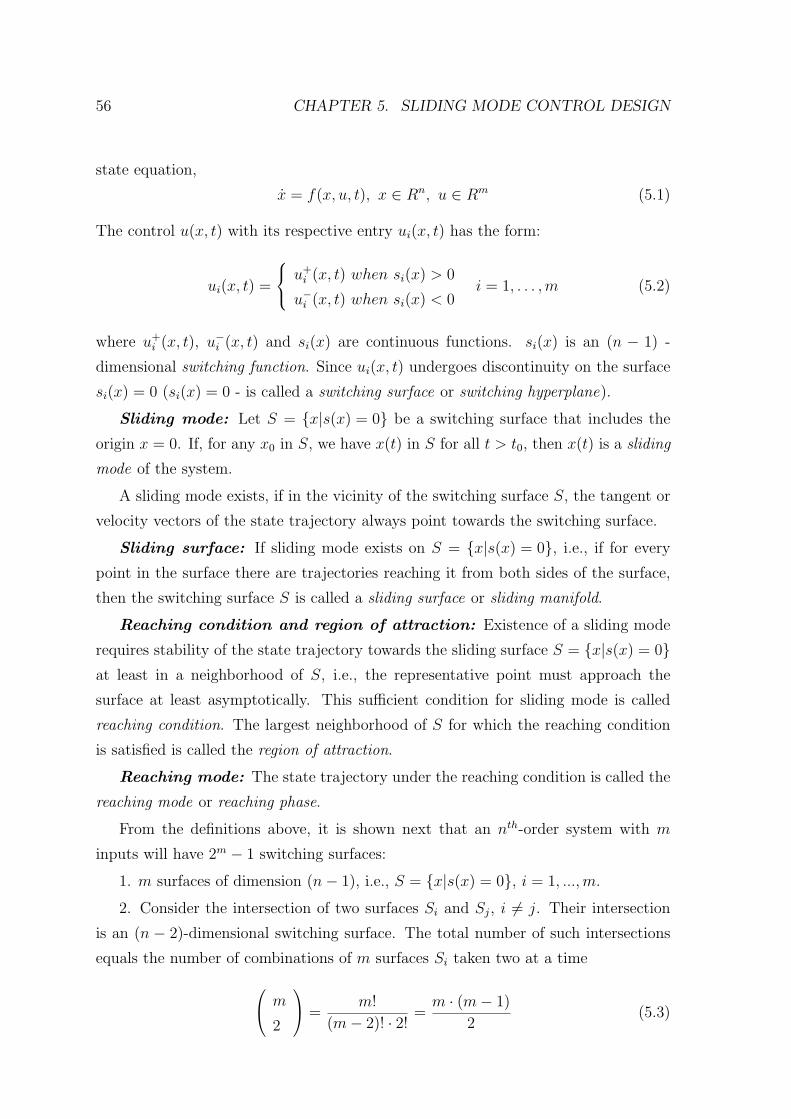
56 CHAPTER 5. SLIDING MODE CONTROL DESIGN
state equation,
x = f(x, u, t), x ∈ Rn, u ∈ Rm (5.1)
The control u(x, t) with its respective entry ui(x, t) has the form:
ui(x, t) =
u+i (x, t) when si(x) > 0
u−i (x, t) when si(x) < 0i = 1, . . . ,m (5.2)
where u+i (x, t), u−i (x, t) and si(x) are continuous functions. si(x) is an (n − 1) -
dimensional switching function. Since ui(x, t) undergoes discontinuity on the surface
si(x) = 0 (si(x) = 0 - is called a switching surface or switching hyperplane).
Sliding mode: Let S = x|s(x) = 0 be a switching surface that includes the
origin x = 0. If, for any x0 in S, we have x(t) in S for all t > t0, then x(t) is a sliding
mode of the system.
A sliding mode exists, if in the vicinity of the switching surface S, the tangent or
velocity vectors of the state trajectory always point towards the switching surface.
Sliding surface: If sliding mode exists on S = x|s(x) = 0, i.e., if for every
point in the surface there are trajectories reaching it from both sides of the surface,
then the switching surface S is called a sliding surface or sliding manifold.
Reaching condition and region of attraction: Existence of a sliding mode
requires stability of the state trajectory towards the sliding surface S = x|s(x) = 0
at least in a neighborhood of S, i.e., the representative point must approach the
surface at least asymptotically. This sufficient condition for sliding mode is called
reaching condition. The largest neighborhood of S for which the reaching condition
is satisfied is called the region of attraction.
Reaching mode: The state trajectory under the reaching condition is called the
reaching mode or reaching phase.
From the definitions above, it is shown next that an nth-order system with m
inputs will have 2m − 1 switching surfaces:
1. m surfaces of dimension (n− 1), i.e., S = x|s(x) = 0, i = 1, ...,m.
2. Consider the intersection of two surfaces Si and Sj, i 6= j. Their intersection
is an (n − 2)-dimensional switching surface. The total number of such intersections
equals the number of combinations of m surfaces Si taken two at a time
m
2
=m!
(m− 2)! · 2!=m · (m− 1)
2(5.3)
5.1. DEFINITIONS AND PRELIMINARIES 57
These switching surfaces are mathematically described by Sij = Si∩Sj, i, j = 1, ...,m,
i 6= j. A geometric interpretation is shown in Fig. 5.1. The intersection of the two
planes, Si and Sj, is the switching surface Sij, which is a line.
Figure 5.1: Geometric interpretation of two intersecting switching surfaces.
3. The intersection of three surfaces Si, Sj and Sk is a switching surface Sijk of
dimension (n − 3). There are
m
3
of such surfaces; Sijk = Si ∩ Sj ∩ Sk, i, j, k =
1, ...,m, i 6= j 6= k.
.......
4. Finally, there is a single switching surface SE of dimension (n −m), which is
the intersection of all surfaces Si, i = 1, ...,m taken together. The surface is given by
SE = x|s(x) = 0 = S1 ∩ S2 ∩ ... ∩ Sm.
Therefore, it is possible to have 2m−1 different sliding modes in such a system. The
sliding mode associated with is called the eventual sliding mode [81]. Many authors
consider only the motion on SE as the sliding motion. However, there are many ways
in which a sliding motion can begin, and these are called switching schemes.
Having defined all the basic concepts, the most commonly used design procedures
of SMC are presented in the following sub-sections. Normally, the design of SMC con-
sists of two parts: First, the sliding surface, which is usually of lower order than the
given process, must be constructed such that the system performance during sliding
mode satisfies the design objectives, in terms of stability, performance index mini-
mization, linearization of nonlinearities, order reduction, etc. Second, the switched
feedback control is designed such that it satisfies the reaching condition and thus
drives the state trajectory to the sliding surface in finite time and maintains it there
thereafter.
58 CHAPTER 5. SLIDING MODE CONTROL DESIGN
5.2 Sliding Surface Design
Sliding surfaces can be either linear or nonlinear. The theory of designing linear
switching surfaces for linear dynamics system has been developed in great depth and
completeness while the design of sliding surfaces for more general nonlinear systems
remains a largely open problem. Some common methods for defining the differential
equation of sliding mode are summarized here.
Consider a general system
x = A(x) +B(x) · u (5.4)
with a sliding surface
S = x|s(x) = 0 (5.5)
where A(x), B(x) are general nonlinear functions of x, and x ∈ Rn, u ∈ Rm.
Canonic form: [82] For a linear single input system, if the system model can
be transformed to controllable canonic form
xi = xi+1, i = 1, ..., n− 1
xn = −∑n
i=1 ai · xi + b · u(5.6)
the sliding surface can be defined by
s =∂s
∂x· x =
∂s
∂xs(x) = Λ · x = λ1 · x1 + λ2 · x2 + ...+ xn = 0 (5.7)
where λi = const, i = 1, 2, ..., n − 1. The coefficients in the switch function (5.7)
define the desired characteristics of the sliding mode, i.e., the characteristics of the
closed loop system after the reaching phase.
Coordinate transformation [83]: If the system (5.4) is linear and described
x = A · x+B · u (5.8)
suppose there exists a nonsingular transformation Q such that
Q ·B =
0
B2
(5.9)
5.2. SLIDING SURFACE DESIGN 59
where B2 is m×m and nonsingular. The system is then transformed to
x1 = A11x1 + A12x2
x2 = A21x1 + A22x2 +B2u(5.10)
where x1 ∈ Rn−m, x2 ∈ Rm. The switching surface can be written as s(x) = Λ1 ·
x1 + Λ2 · x2. Without loss of generality, we can assume that Λ2 is nonsingular, and
in sliding mode we have Λ1 · x1 + Λ2 · x2 = 0, i.e., x2 is related linearly to x1 and the
system satisfies
x1 = A11x1 + A12x2
x2 = −Kx1
(5.11)
where K = Λ−12 ·Λ1. (5.11) represents an (n−m)th order system in which x2 is viewed
as the control input to the constrained system, hence the dynamic behavior of the
sliding mode is determined by
x1 = (A11 − A12 ·K) · x1 (5.12)
The above procedures show that the design of an appropriate sliding surface has
been transformed to a reduced-order state feedback design problem. In general, if
the pair (A,B) is controllable, (A11, A12) is also controllable, thus it is possible to use
classical feedback design, e.g., pole placement or linear quadratic methods to compute
K such that A11 − A12 ·K has desired characteristics. Having found K, the desired
switching function can be designed as
s(x) = Λ · x = Λ2 · [K, I] · x (5.13)
where Λ2 can be selected arbitrary. A simple selection is to let Λ2 = I
The linear quadratic (LQ) approach [83]: For linear time-invariant systems,
optimal sliding mode, or more precisely, optimal choice of the vector K of (5.13)
can be obtained by minimising a quadratic cost over an infinite time interval. For
example, since x2 can be regarded as the input of the system (5.11), LQ optimization
can be used to find the optimal sliding mode for (5.11) by minimizing
J =∫ ∞
ts
(
xT1 ·Q11 · x1 + 2xT
1 ·Q12 · x2 + xT2 ·Q22 · x2
)
dt (5.14)
Without loss of generality, we can let Q12 = 0, and then the optimal control x2 is
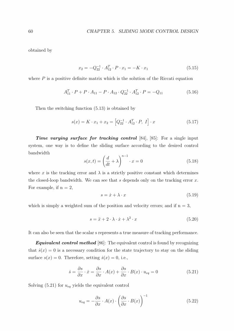
60 CHAPTER 5. SLIDING MODE CONTROL DESIGN
obtained by
x2 = −Q−122 · A
T12 · P · x1 = −K · x1 (5.15)
where P is a positive definite matrix which is the solution of the Riccati equation
AT11 · P + P · A11 − P · A12 ·Q
−122 · A
T12 · P = −Q11 (5.16)
Then the switching function (5.13) is obtained by
s(x) = K · x1 + x2 =[
Q−122 · A
T12 · P, I
]
· x (5.17)
Time varying surface for tracking control [84], [85]: For a single input
system, one way is to define the sliding surface according to the desired control
bandwidth
s(x, t) =
(
d
dt+ λ
)n−1
· x = 0 (5.18)
where x is the tracking error and λ is a strictly positive constant which determines
the closed-loop bandwidth. We can see that s depends only on the tracking error x.
For example, if n = 2,
s = x+ λ · x (5.19)
which is simply a weighted sum of the position and velocity errors; and if n = 3,
s = x+ 2 · λ · x+ λ2 · x (5.20)
It can also be seen that the scalar s represents a true measure of tracking performance.
Equivalent control method [86]: The equivalent control is found by recognizing
that s(x) = 0 is a necessary condition for the state trajectory to stay on the sliding
surface s(x) = 0. Therefore, setting s(x) = 0, i.e.,
s =∂s
∂x· x =
∂s
∂x· A(x) +
∂s
∂x·B(x) · ueq = 0 (5.21)
Solving (5.21) for ueq yields the equivalent control
ueq = −∂s
∂x· A(x) ·
(
∂s
∂x·B(x)
)−1
(5.22)
5.2. SLIDING SURFACE DESIGN 61
where ∂s∂x·B(x) is nonsingular.
The dynamics of the system is governed by:
x =
I −B(x) ·
(
∂s
∂x·B(x)
)−1
·∂s
∂x
· A(x) (5.23)
If the system (5.4) is linear and described by
x = A · x+B · u (5.24)
where A and B are properly dimensioned constant matrices, then the switch surface
can be defined as
s(x) = Λ · x(t) = 0 (5.25)
i.e., ∂s∂x
= Λ, where Λ = [λ1, ..., λm]T is a m× n matrix, and then we have:
ueq = − (Λ ·B)−1 · Λ · A · x (5.26)
and (5.23) becomes
x =(
I −B · (Λ ·B)−1 · Λ)
· A · x (5.27)
Equations (5.23) and (5.27) describe the behavior of the systems (5.4) and (5.24),
respectively, which are restricted to the switching surface if the initial condition x(t0)
satisfies s(x(t0)) = 0. For the linear case, the system dynamics is ensured by a suitable
choice of the feedback matrix K = (Λ ·B)−1 ·Λ ·A. In other words, the choice of the
matrix Λ can be made without prior knowledge of the form of the control vector u.
Dynamic sliding surface/frequency-shaped sliding surface [87]: The slid-
ing surfaces designed above are all static, i.e., they are different linear combinations
of the state variables. Young and Ozguner in [87] proposed a new type of switching
surface which appears as a linear operator. The purpose of the design was to atten-
uate high frequency components in the error dynamics, thus to avoid vibrations due
to the interaction of sliding mode and unmodelled dynamics of the system.
Other methods for design of both linear and nonlinear sliding surfaces can also
be found in the literature, such as designing robust sliding hyperplanes via a Riccati
approach (Kim, et al., 2000), constructing a discontinuous surface for VSS by a
Lyapunov approach (Su, et al., 1996b) and designing an adaptive sliding surface for
model reference VSC (Nonaka, et al., 1996; Yao and Tomizuka, 1994; Su and Leung,
62 CHAPTER 5. SLIDING MODE CONTROL DESIGN
1993; Bartolini, et al.,1997; Bartolini and Ferrara,1999).
5.3 Control Law Design
Once the sliding surfaces have been selected, attention must be turned to solving
the reachability problem. This involves the selection of a state feedback control
function u : Rn → Rm which can drive the state x towards the surface and thereafter
maintains it on the surface. In other words, the controlled system must satisfy the
reaching conditions. For general MIMO systems, different switching schemes use
different reaching laws during approach of the sliding mode. The commonly used
reaching laws and the developed control methods were summarized in [81] and [88].
Reaching laws
For both SISO and MIMO systems, the commonly used reaching conditions are
specified in the following forms:
- The direct switching function approach
The classic sufficient condition for sliding mode to appear is to satisfy the condition
si · si < 0, i = 1, ...,m (5.28)
and a similar condition was also proposed in [82], i.e.,
limsi→0+ si < 0 and limsi→0− si > 0 (5.29)
These reaching laws result in a VSC where individual switching surfaces and their
intersection are all sliding surfaces. This reaching is global but does not guarantee
finite reaching time.
- The Lyapunov function approach
Choosing the Lyapunov function candidate
V (x, t) =1
2· sT · s (5.30)
The global reaching condition is then given by
V (x, t) < 0 (5.31)
This reaching law results in a VSC where sliding mode is guaranteed only on the
5.3. CONTROL LAW DESIGN 63
intersection of all switching surfaces, i.e., the eventual sliding mode, whereas points
on the individual switching surfaces may or may not belong to the sliding surface.
Finite reaching time can be guaranteed if (5.31) is modified to V (x, t) < −ǫ, ǫ is
strictly positive.
- Gao’s reaching law approach Gao and Hung in [89] proposed a reaching law which
directly specifies the dynamics of the switching surface by the differential equation
s = −Q · sgn(s)− P · h(s) (5.32)
where
Q = diag [q1, q2, ..., qm] , qi > 0, i = 1, 2, ...,m
P = diag [p1, p2, ..., pm] , pi > 0, i = 1, 2, ...,m
and
sgn(s) = [sgn(s1), sgn(s2), ..., sgn(sm)]T
h(s) = [h1(s1), h2(s2), ..., hm(sm)]T
si · hi(s) > 0, hi(0) = 0.
Three practical special cases of (5.32) are given below.
A. Constant rate reaching
s = −Q · sgn(s) (5.33)
This law forces the switching variable s(x) to reach the switching manifold S at a
constant rate |si| = −qi. The merit of this reaching law is its simplicity. But, as we
know, if qi is too small, the reaching time will be too long. On the other hand, a too
large qi will cause severe chattering.
B. Constant plus proportional rate reaching
s = −Q · sgn(s)− P · s (5.34)
Clearly, by adding the proportional rate term −P · s, the state is forced to approach
the switching manifolds faster when s is large. It can be shown that the reaching
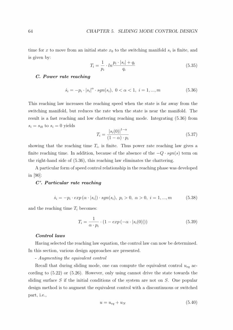
64 CHAPTER 5. SLIDING MODE CONTROL DESIGN
time for x to move from an initial state x0 to the switching manifold si is finite, and
is given by:
Ti =1
pi
· lnpi · |si|+ qi
qi(5.35)
C. Power rate reaching
si = −pi · |si|α · sgn(si), 0 < α < 1, i = 1, ...,m (5.36)
This reaching law increases the reaching speed when the state is far away from the
switching manifold, but reduces the rate when the state is near the manifold. The
result is a fast reaching and low chattering reaching mode. Integrating (5.36) from
si = si0 to si = 0 yields
Ti =|si(0)|1−α
(1− α) · pi
(5.37)
showing that the reaching time Ti, is finite. Thus power rate reaching law gives a
finite reaching time. In addition, because of the absence of the −Q · sgn(s) term on
the right-hand side of (5.36), this reaching law eliminates the chattering.
A particular form of speed control relationship in the reaching phase was developed
in [90]:
C’. Particular rate reaching
si = −pi · exp (α · |si|) · sgn(si), pi > 0, α > 0, i = 1, ...,m (5.38)
and the reaching time Ti becomes:
Ti =1
α · pi
· (1− exp (−α · |si(0)|)) (5.39)
Control laws
Having selected the reaching law equation, the control law can now be determined.
In this section, various design approaches are presented.
- Augmenting the equivalent control
Recall that during sliding mode, one can compute the equivalent control ueq ac-
cording to (5.22) or (5.26). However, only using cannot drive the state towards the
sliding surface S if the initial conditions of the system are not on S. One popular
design method is to augment the equivalent control with a discontinuous or switched
part, i.e.,
u = ueq + uN (5.40)
5.3. CONTROL LAW DESIGN 65
where uN is added to satisfy the reaching condition which may have different forms.
For a controller having the structure of (5.40), we have
s(x) = ∂s∂x· x = ∂s
∂x· [A(x) +B(x) · (ueq + uN)]
= ∂s∂x· [A(x) +B(x) · ueq] + ∂s
∂x·B(x) · uN
= ∂s∂x·B(x) · uN
(5.41)
For simplicity, assume ∂s∂x·B(x) = I, the identity. Then s(x) = uN . According to [88]
some often used forms of uN are given below
A - Relay with gains
uN =
−α · sgn(s),
0,
s 6= 0, α > 0
s = 0,(5.42)
α can be either a constant matrix or state dependent α(x). Each control unit uNi
meets the reaching condition since
si · si = −α · si(x) · sgn(si(x)) < 0, for si(x) 6= 0 (5.43)
B - Linear feedback with switching gains
uNi = ψ · x; ψ = [ψij] , ψij =
−αij, si · xj > 0
βij, si · xj < 0(5.44)
with αij, βij > 0. The reaching condition is satisfied with
si · si = si · (ψi1 · x1 + ψi2 · x2 + ...+ ψin · xn) < 0 (5.45)
C - Linear continuous feedback
uN = −α · s(x) (5.46)
where α is defined in the same way as above, and hence the reaching condition is
si · si = −α · s2i (x) < 0 (5.47)
66 CHAPTER 5. SLIDING MODE CONTROL DESIGN
D - Univector nonlinearity with scalar factor
uN = −s(x)
‖s(x)‖· γ (5.48)
where γ > 0 is a scalar. Thus the reaching condition is satisfied with
s(x) · sT (x) = −‖s(x)‖ · γ < 0 if s(x) 6= 0 (5.49)
- The reaching law method
By using the reaching law approach proposed in [81], the control can be directly
obtained by computing the time derivative s(x) of along the reaching mode trajectory,
i.e.,
s =∂s
∂x· (A(x) +B(x) · u) = −Q · sgn(s)− P · h(s) (5.50)
Thus, we have
u = −
(
∂s
∂x· A(x) +Q · sgn(s) + P · h(s)
)
·
(
∂s
∂x·B(x)
)T
(5.51)
By this approach, the resulting sliding mode is not preassigned but follows the natural
trajectory on a first-reach-first-switch scheme. The switching takes place depending
on the location of the initial state.
- Control hierarchy method
The hierarchical control method uses the first reaching law i.e., the classical suffi-
cient condition for a sliding mode. This method is used to establish a control scheme,
such that sliding modes take place in a preassigned order, i.e., the system state starts
from the initial condition x0, moves progressively onto lower dimensional switching
surfaces and eventually reaches the final sliding surface SE:
x0 → S1 → (S1 ∩ S2)→ (S1 ∩ S2 ∩ S3)→ ...→ SE
The disadvantage of this method is that the control is determined by a set of
complicated inequalities. For example, for the system (5.24), the determination of
the control u involves the solution of m pairs of inequalities,
si =∂si
∂x· (A · x+B · u) =
> 0, when si < 0
< 0, when si > 0, i = 1, ...,m (5.52)
Solving (5.52) is usually a very difficult task. As a result, the scheme is seldom used.
5.4. CHATTERING PROBLEM AND ITS REDUCTION 67
5.4 Chattering Problem and its Reduction
It has already been mentioned that to guarantee the desired behaviour of the close-
loop system, the sliding mode controllers require an infinitely fast switching mecha-
nism. However, due to physical limitations in real-world systems, directly applying
the above developed control algorithms will always lead to oscillations in some vicin-
ity of the switching surface, i.e., the so called chattering phenomenon. There are two
possible mechanisms which produce chattering (Young, et al., 1999). First, chattering
may be caused by the switching nonidealities, such as time delays or time constants,
which exist in any implementation of switching devices, typically including both ana-
log and digital circuits as well as microprocessor based implementations. Second,
even if the switching device is considered ideal and capable of switching at an infi-
nite frequency, the presence of parasitic dynamics, i.e., unmodelled dynamics, also
causes chattering to appear in the neighborhood of the sliding surface. The parasitic
dynamics are those of fast dynamics of actuators, sensors and other high frequency
modes of the controlled process, which are usually neglected in the open-loop model
used for control design if the associated poles are well damped and outside the de-
sired bandwidth of the feedback control system. However, in sliding mode controlled
systems, due to the discontinuity of the control signal, the interactions between the
parasitic dynamics and the switching term may result in a nondecaying oscillation
with finite amplitude and frequency, i.e., chattering. If the switching gain is large,
such kind of chattering may even cause unpredictable instability.
The chattering problem is considered as a major obstacle for SMC to become a
more appreciated control method among practicing control engineers. To reduce the
chattering effect has long been a major objective in research on SMC. The existing
approaches for chattering reduction in design of SMC are summarized in the following.
Boundary layer control [84], [85]: A boundary layer around the sliding surface
is specified. Inside the boundary layer, the switching function is usually replaced by
a linear feedback gain, thus the control signal becomes continuous and chattering is
avoided. The shortcoming of this approach is that the robustness properties of the
sliding mode are actually lost inside the boundary layer, such that uncertainties and
parasitic dynamics must be carefully considered and modeled in the feedback design
in order to avoid instability.
Observer-based sliding mode control [86], [91], [92]: This approach utilizes
asymptotic state observers to construct a high frequency by pass loop, i.e., the control
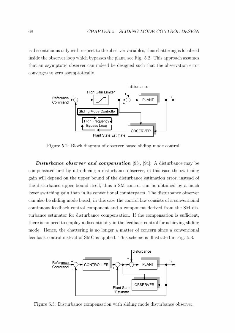
68 CHAPTER 5. SLIDING MODE CONTROL DESIGN
is discontinuous only with respect to the observer variables, thus chattering is localized
inside the observer loop which bypasses the plant, see Fig. 5.2. This approach assumes
that an asymptotic observer can indeed be designed such that the observation error
converges to zero asymptotically.
Figure 5.2: Block diagram of observer based sliding mode control.
Disturbance observer and compensation [93], [94]: A disturbance may be
compensated first by introducing a disturbance observer, in this case the switching
gain will depend on the upper bound of the disturbance estimation error, instead of
the disturbance upper bound itself, thus a SM control can be obtained by a much
lower switching gain than in its conventional counterparts. The disturbance observer
can also be sliding mode based, in this case the control law consists of a conventional
continuous feedback control component and a component derived from the SM dis-
turbance estimator for disturbance compensation. If the compensation is sufficient,
there is no need to employ a discontinuity in the feedback control for achieving sliding
mode. Hence, the chattering is no longer a matter of concern since a conventional
feedback control instead of SMC is applied. This scheme is illustrated in Fig. 5.3.
Figure 5.3: Disturbance compensation with sliding mode disturbance observer.
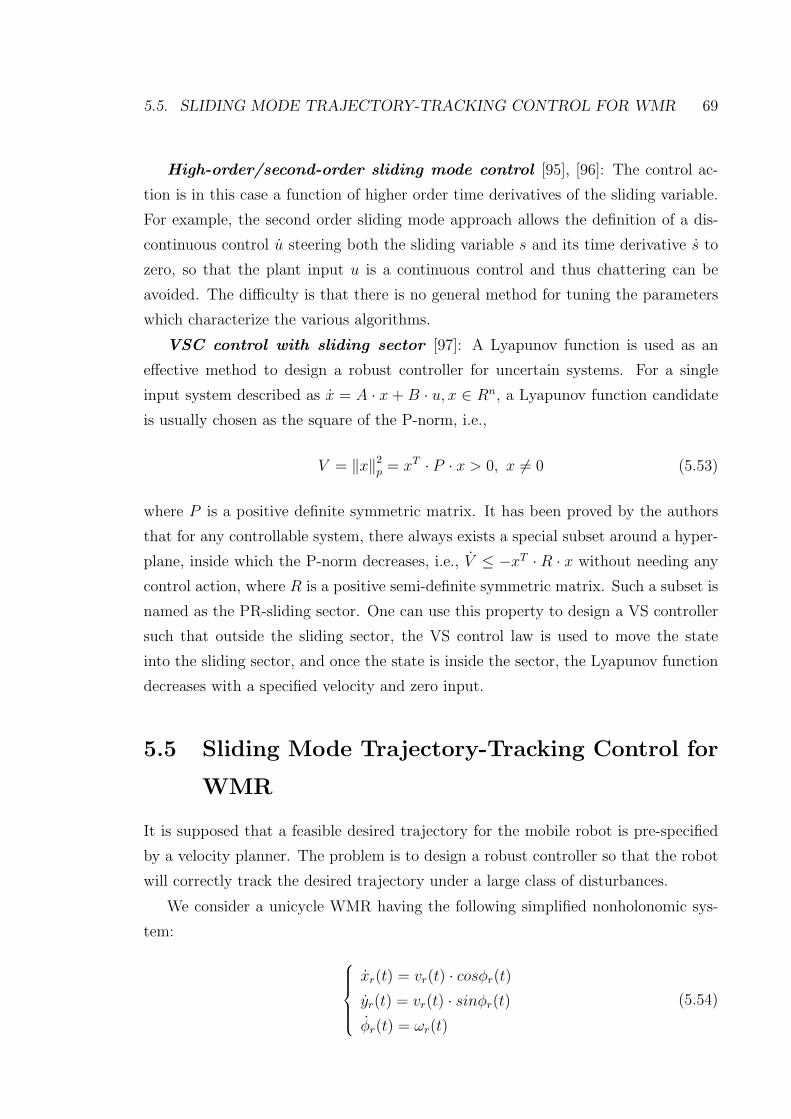
5.5. SLIDING MODE TRAJECTORY-TRACKING CONTROL FOR WMR 69
High-order/second-order sliding mode control [95], [96]: The control ac-
tion is in this case a function of higher order time derivatives of the sliding variable.
For example, the second order sliding mode approach allows the definition of a dis-
continuous control u steering both the sliding variable s and its time derivative s to
zero, so that the plant input u is a continuous control and thus chattering can be
avoided. The difficulty is that there is no general method for tuning the parameters
which characterize the various algorithms.
VSC control with sliding sector [97]: A Lyapunov function is used as an
effective method to design a robust controller for uncertain systems. For a single
input system described as x = A · x + B · u, x ∈ Rn, a Lyapunov function candidate
is usually chosen as the square of the P-norm, i.e.,
V = ‖x‖2p = xT · P · x > 0, x 6= 0 (5.53)
where P is a positive definite symmetric matrix. It has been proved by the authors
that for any controllable system, there always exists a special subset around a hyper-
plane, inside which the P-norm decreases, i.e., V ≤ −xT · R · x without needing any
control action, where R is a positive semi-definite symmetric matrix. Such a subset is
named as the PR-sliding sector. One can use this property to design a VS controller
such that outside the sliding sector, the VS control law is used to move the state
into the sliding sector, and once the state is inside the sector, the Lyapunov function
decreases with a specified velocity and zero input.
5.5 Sliding Mode Trajectory-Tracking Control for
WMR
It is supposed that a feasible desired trajectory for the mobile robot is pre-specified
by a velocity planner. The problem is to design a robust controller so that the robot
will correctly track the desired trajectory under a large class of disturbances.
We consider a unicycle WMR having the following simplified nonholonomic sys-
tem:
xr(t) = vr(t) · cosφr(t)
yr(t) = vr(t) · sinφr(t)
φr(t) = ωr(t)
(5.54)
70 CHAPTER 5. SLIDING MODE CONTROL DESIGN
where xr and yr are the Cartesian coordinates of the geometric center, vr is the linear
velocity, φr is the vehicle’s heading angle and ωr is the angular velocity (see Figure
3.1).
The trajectory tracking errors can be described by (xe, ye, φe). The aim of this
section is to design a stable controller that generates a command vector (vc,ωc).
From Figure 3.6, the error vector for trajectory-tracking is
xe
ye
φe
=
cosφd sinφd 0
−sinφd cosφd 0
0 0 1
·
xr − xd
yr − yd
φr − φd
(5.55)
where: (xd, yd, φd) is the virtual robot pose.
The corresponding error derivatives are:
xe = −vd + vr · cosφe + ye · ωd
ye = vr · sinφe − xe · ωd
φe = ωr − ωd
(5.56)
where vd and ωd are the desired linear and angular velocities, respectively.
In this thesis it is assumed that |φe| < π/2, which means that the robot orientation
must not be perpendicular to the desired trajectory.
We propose a new design of sliding surface such that lateral error, ye, and angular
variable, φe, are internally coupled with each other in a sliding surface leading to
convergence of both variables. For that purpose the following sliding surfaces are
proposed:
s1 = xe + k1 · xe (5.57)
s2 = ye + k2 · ye + k0 · sgn(ye) · φe (5.58)
where k0, k1, k2 are positive constant parameters, xe, ye and θe are the trajectory-
tracking errors defined in (5.55).
If s1 converges to zero, trivially xe converges to zero. If s2 converges to zero, in
steady-state it becomes ye = −k2 · ye − k0 · sgn(ye) · φe. For ye < 0 ⇒ ye > 0 if only
if k0 < k2 · |ye| / |φe|. For ye > 0 ⇒ ye < 0 if only if k0 < k2 · |ye| / |φe|. Finally, it can
be known from s2 that convergence of ye and ye leads to convergence of φe to zero.
A practical general form of reaching the control law is:
5.5. SLIDING MODE TRAJECTORY-TRACKING CONTROL FOR WMR 71
s = −Q · s− P · sgn(s) (5.59)
where Q and P are positive constant values. By adding the proportional rate
term −Q · s, the state is forced to approach the switching manifold faster when s is
large.
From the time derivations of (5.57) and (5.58), and knowing that
φe = φr − φd = ωr − ωd
after some mathematical manipulation one achieves
vc =−Q1 · s1 − P1 · sgn(s1)− k1 · xe − ωd · ye − ωd · ye + vr · φe · sinφe + vd
cosφe
(5.60)
ωc =−Q2 · s2 − P2 · sgn(s2)− k2 · ye − vr · sinφe + ωd · xe + ωd · xe
vr · cosφe + k0 · sgn(ye)+ ωd (5.61)
Let us define V = 12· sT · s as a Lyapunov function candidate, therefore its time
derivative is
V = s1 · s1 + s2 · s2 = s1 · (−Q1 · s1 − P1 · sgn(s1)) + s2 · (−Q2 · s2 − P2 · sgn(s2)) =
= −sT ·Q · s− P1 · |s1| − P2 · |s2|
For V to be negative semi-definite, it is sufficient to choose Qi and Pi such that
Qi, Pi ≥ 0.
5.5.1 Simulation Results
In this subsection, simulation results of the proposed method are presented. The
simulation model block diagrams are shown in Figs. 5.4 and 5.5.
Figures 5.7 and 5.8 were automatically generated by the trajectory planner de-
scribed in Chapter 4. These profiles are generated respecting the human comfort
condition (aw < 0.31 m/s2). This result can be observed in the graphics shown in
Fig. 5.8, which are related with the trajectories shown in Fig. 5.6.
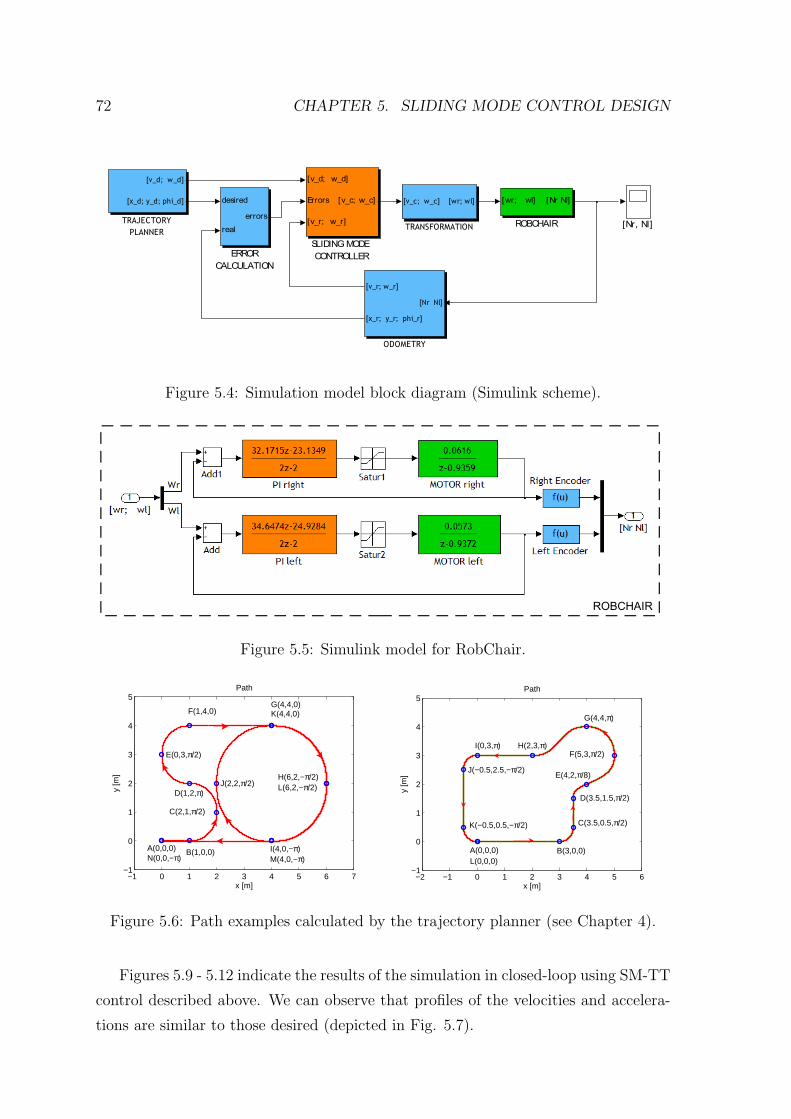
72 CHAPTER 5. SLIDING MODE CONTROL DESIGN
Figure 5.4: Simulation model block diagram (Simulink scheme).
Figure 5.5: Simulink model for RobChair.
−1 0 1 2 3 4 5 6 7−1
0
1
2
3
4
5Path
x [m]
y [m
]
J(2,2,π/2)
B(1,0,0)
C(2,1,π/2)
D(1,2,π)
E(0,3,π/2)
F(1,4,0)G(4,4,0)K(4,4,0)
H(6,2,−π/2)L(6,2,−π/2)
I(4,0,−π)M(4,0,−π)
A(0,0,0)N(0,0,−π)
−2 −1 0 1 2 3 4 5 6−1
0
1
2
3
4
5Path
x [m]
y [m
]
A(0,0,0) B(3,0,0)
C(3.5,0.5,π/2)
D(3.5,1.5,π/2)
E(4,2,π/8)
F(5,3,π/2)
G(4,4,π)
H(2,3,π)I(0,3,π)
J(−0.5,2.5,−π/2)
K(−0.5,0.5,−π/2)
L(0,0,0)
Figure 5.6: Path examples calculated by the trajectory planner (see Chapter 4).
Figures 5.9 - 5.12 indicate the results of the simulation in closed-loop using SM-TT
control described above. We can observe that profiles of the velocities and accelera-
tions are similar to those desired (depicted in Fig. 5.7).
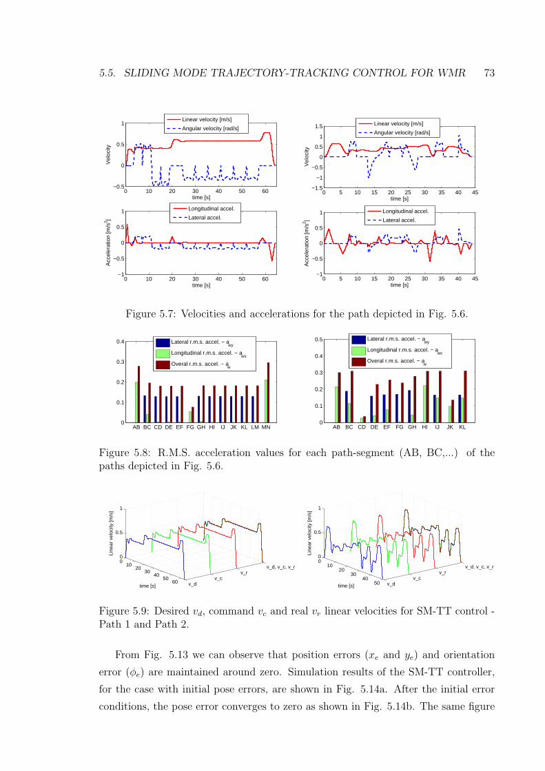
5.5. SLIDING MODE TRAJECTORY-TRACKING CONTROL FOR WMR 73
0 10 20 30 40 50 60−0.5
0
0.5
1
time [s]
Vel
ocity
Linear velocity [m/s]
Angular velocity [rad/s]
0 10 20 30 40 50 60−1
−0.5
0
0.5
1
time [s]
Acc
eler
atio
n [m
/s2 ]
Longitudinal accel.
Lateral accel.
0 5 10 15 20 25 30 35 40 45−1.5
−1
−0.5
0
0.5
1
1.5
time [s]
Vel
ocity
Linear velocity [m/s]
Angular velocity [rad/s]
0 5 10 15 20 25 30 35 40 45−1
−0.5
0
0.5
1
time [s]
Acc
eler
atio
n [m
/s2 ]
Longitudinal accel.
Lateral accel.
Figure 5.7: Velocities and accelerations for the path depicted in Fig. 5.6.
AB BC CD DE EF FG GH HI IJ JK KL LM MN0
0.1
0.2
0.3
0.4
Lateral r.m.s. accel. − awy
Longitudinal r.m.s. accel. − awx
Overal r.m.s. accel. − aw
AB BC CD DE EF FG GH HI IJ JK KL0
0.1
0.2
0.3
0.4
0.5
Lateral r.m.s. accel. − awy
Longitudinal r.m.s. accel. − awx
Overal r.m.s. accel. − aw
Figure 5.8: R.M.S. acceleration values for each path-segment (AB, BC,...) of thepaths depicted in Fig. 5.6.
v_dv_c
v_rv_d, v_c, v_r
010
2030
4050
60
0
0.5
1
time [s]
Line
ar v
eloc
ity [m
/s]
v_dv_c
v_rv_d, v_c, v_r
010
2030
4050
0
0.5
1
time [s]
Line
ar v
eloc
ity [m
/s]
Figure 5.9: Desired vd, command vc and real vr linear velocities for SM-TT control -Path 1 and Path 2.
From Fig. 5.13 we can observe that position errors (xe and ye) and orientation
error (φe) are maintained around zero. Simulation results of the SM-TT controller,
for the case with initial pose errors, are shown in Fig. 5.14a. After the initial error
conditions, the pose error converges to zero as shown in Fig. 5.14b. The same figure
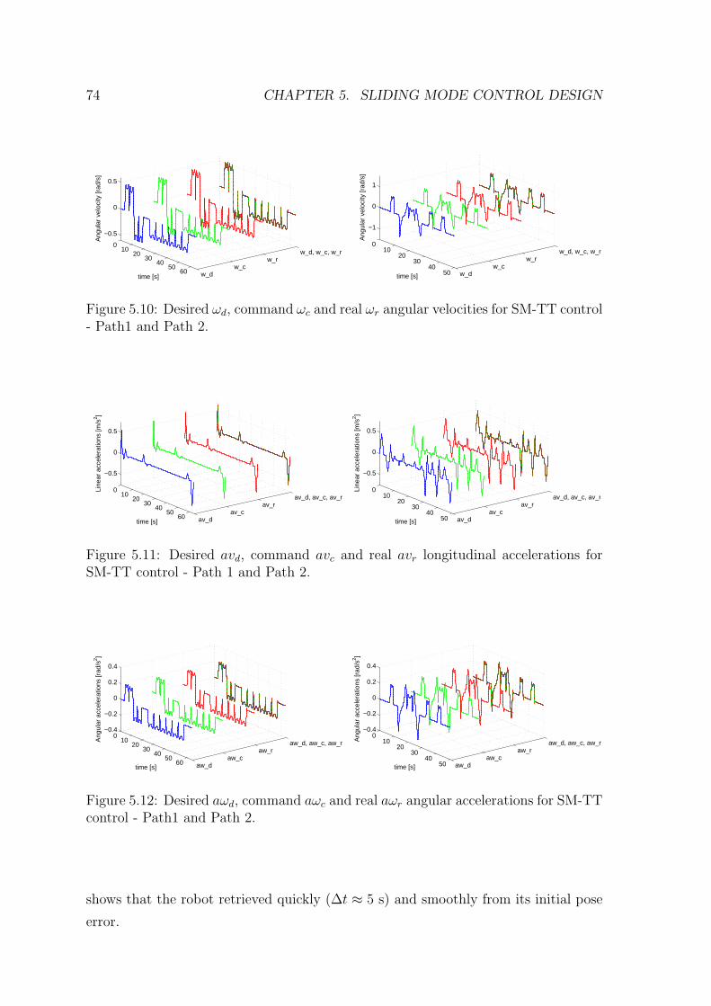
74 CHAPTER 5. SLIDING MODE CONTROL DESIGN
w_dw_c
w_rw_d, w_c, w_r
010
2030
4050
60
−0.5
0
0.5
time [s]
Ang
ular
vel
ocity
[rad
/s]
w_dw_c
w_rw_d, w_c, w_r
010
2030
4050
−1
0
1
time [s]
Ang
ular
vel
ocity
[rad
/s]
Figure 5.10: Desired ωd, command ωc and real ωr angular velocities for SM-TT control- Path1 and Path 2.
av_dav_c
av_rav_d, av_c, av_r
010
2030
4050
60
−0.5
0
0.5
time [s]
Line
ar a
ccel
erat
ions
[m/s
2 ]
av_dav_c
av_rav_d, av_c, av_r
010
2030
4050
−0.5
0
0.5
time [s]
Line
ar a
ccel
erat
ions
[m/s
2 ]
Figure 5.11: Desired avd, command avc and real avr longitudinal accelerations forSM-TT control - Path 1 and Path 2.
aw_daw_c
aw_raw_d, aw_c, aw_r
010
2030
4050
60
−0.4
−0.2
0
0.2
0.4
time [s]
Ang
ular
acc
eler
atio
ns [r
ad/s
2 ]
aw_daw_c
aw_raw_d, aw_c, aw_r
010
2030
4050
−0.4
−0.2
0
0.2
0.4
time [s]
Ang
ular
acc
eler
atio
ns [r
ad/s
2 ]
Figure 5.12: Desired aωd, command aωc and real aωr angular accelerations for SM-TTcontrol - Path1 and Path 2.
shows that the robot retrieved quickly (∆t ≈ 5 s) and smoothly from its initial pose
error.
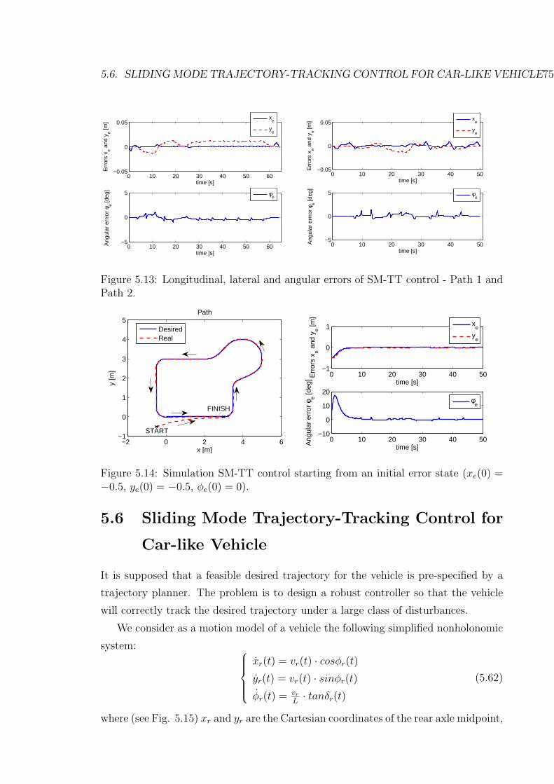
5.6. SLIDING MODE TRAJECTORY-TRACKING CONTROL FOR CAR-LIKE VEHICLE75
0 10 20 30 40 50 60−0.05
0
0.05
time [s]
Err
ors
x e and
ye [m
]
x
e
ye
0 10 20 30 40 50 60−5
0
5
time [s]
Ang
ular
err
ror
φ e [deg
]
φe
0 10 20 30 40 50−0.05
0
0.05
time [s]
Err
ors
x e and
ye [m
]
x
e
ye
0 10 20 30 40 50−5
0
5
time [s]
Ang
ular
err
ror
φ e [deg
]
φe
Figure 5.13: Longitudinal, lateral and angular errors of SM-TT control - Path 1 andPath 2.
−2 0 2 4 6−1
0
1
2
3
4
5Path
x [m]
y [m
]
DesiredReal
START
FINISH
0 10 20 30 40 50−1
0
1
time [s]
Err
ors
x e and
ye [m
]
xe
ye
0 10 20 30 40 50−10
0
10
20
time [s]Ang
ular
err
or φ
e [deg
]
φe
Figure 5.14: Simulation SM-TT control starting from an initial error state (xe(0) =−0.5, ye(0) = −0.5, φe(0) = 0).
5.6 Sliding Mode Trajectory-Tracking Control for
Car-like Vehicle
It is supposed that a feasible desired trajectory for the vehicle is pre-specified by a
trajectory planner. The problem is to design a robust controller so that the vehicle
will correctly track the desired trajectory under a large class of disturbances.
We consider as a motion model of a vehicle the following simplified nonholonomic
system:
xr(t) = vr(t) · cosφr(t)
yr(t) = vr(t) · sinφr(t)
φr(t) = vr
L· tanδr(t)
(5.62)
where (see Fig. 5.15) xr and yr are the Cartesian coordinates of the rear axle midpoint,
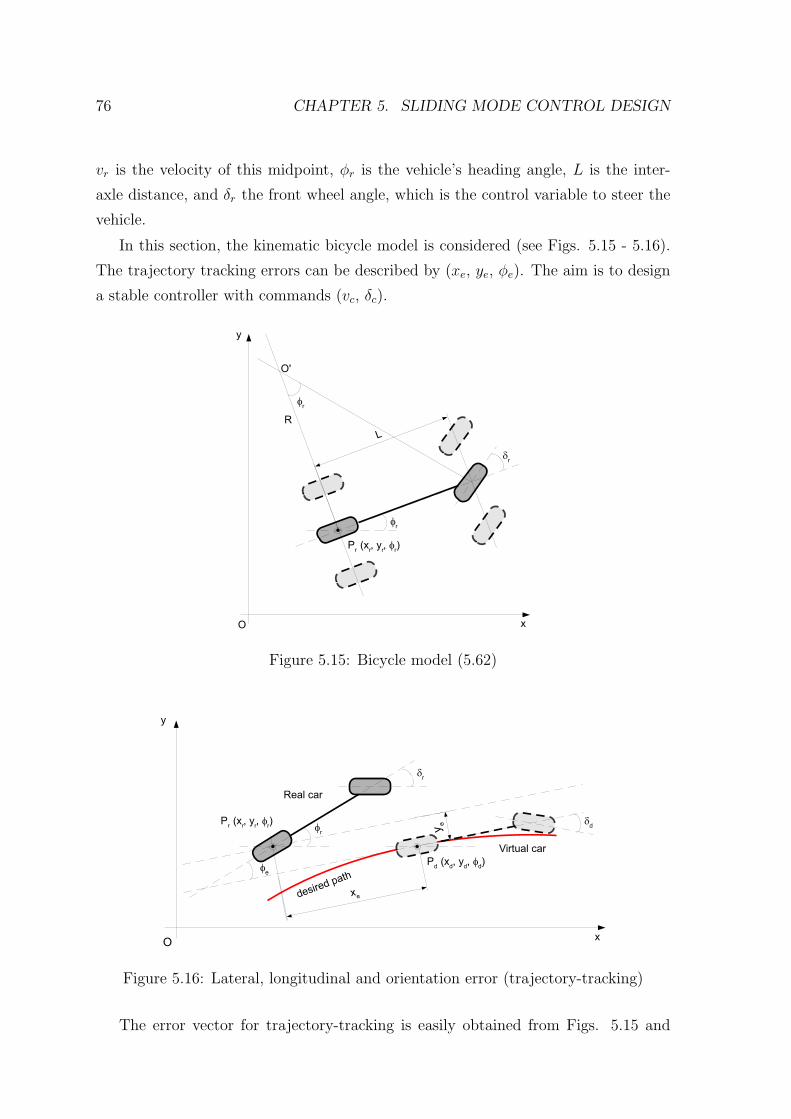
76 CHAPTER 5. SLIDING MODE CONTROL DESIGN
vr is the velocity of this midpoint, φr is the vehicle’s heading angle, L is the inter-
axle distance, and δr the front wheel angle, which is the control variable to steer the
vehicle.
In this section, the kinematic bicycle model is considered (see Figs. 5.15 - 5.16).
The trajectory tracking errors can be described by (xe, ye, φe). The aim is to design
a stable controller with commands (vc, δc).
Figure 5.15: Bicycle model (5.62)
Figure 5.16: Lateral, longitudinal and orientation error (trajectory-tracking)
The error vector for trajectory-tracking is easily obtained from Figs. 5.15 and
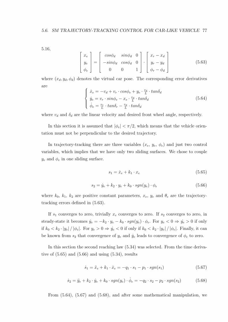
5.6. SM TRAJECTORY-TRACKING CONTROL FOR CAR-LIKE VEHICLE 77
5.16,
xe
ye
φe
=
cosφd sinφd 0
−sinφd cosφd 0
0 0 1
·
xr − xd
yr − yd
φr − φd
(5.63)
where (xd, yd, φd) denotes the virtual car pose. The corresponding error derivatives
are
xe = −vd + vr · cosφe + ye ·vd
L· tanδd
ye = vr · sinφe − xe ·vd
L· tanδd
φe = vr
L· tanδr −
vd
L· tanδd
(5.64)
where vd and δd are the linear velocity and desired front wheel angle, respectively.
In this section it is assumed that |φe| < π/2, which means that the vehicle orien-
tation must not be perpendicular to the desired trajectory.
In trajectory-tracking there are three variables (xe, ye, φe) and just two control
variables, which implies that we have only two sliding surfaces. We chose to couple
ye and φe in one sliding surface.
s1 = xe + k1 · xe (5.65)
s2 = ye + k2 · ye + k0 · sgn(ye) · φe (5.66)
where k0, k1, k2 are positive constant parameters, xe, ye and θe are the trajectory-
tracking errors defined in (5.63).
If s1 converges to zero, trivially xe converges to zero. If s2 converges to zero, in
steady-state it becomes ye = −k2 · ye − k0 · sgn(ye) · φe. For ye < 0 ⇒ ye > 0 if only
if k0 < k2 · |ye| / |φe|. For ye > 0 ⇒ ye < 0 if only if k0 < k2 · |ye| / |φe|. Finally, it can
be known from s2 that convergence of ye and ye leads to convergence of φe to zero.
In this section the second reaching law (5.34) was selected. From the time deriva-
tive of (5.65) and (5.66) and using (5.34), results
s1 = xe + k1 · xe = −q1 · s1 − p1 · sgn(s1) (5.67)
s2 = ye + k2 · ye + k0 · sgn(ye) · φe = −q2 · s2 − p2 · sgn(s2) (5.68)
From (5.64), (5.67) and (5.68), and after some mathematical manipulation, we
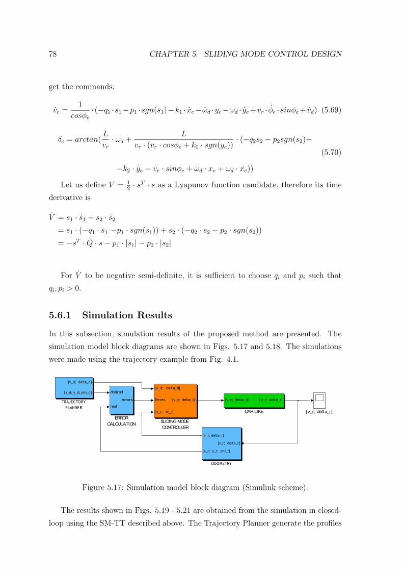
78 CHAPTER 5. SLIDING MODE CONTROL DESIGN
get the commands:
vc =1
cosφe
· (−q1 ·s1−p1 ·sgn(s1)−k1 · xe− ωd ·ye−ωd · ye +vr · φe ·sinφe + vd) (5.69)
δc = arctan(L
vr
· ωd +L
vr · (vr · cosφe + k0 · sgn(ye))· (−q2s2 − p2sgn(s2)−
−k2 · ye − vr · sinφe + ωd · xe + ωd · xe))
(5.70)
Let us define V = 12· sT · s as a Lyapunov function candidate, therefore its time
derivative is
V = s1 · s1 + s2 · s2
= s1 · (−q1 · s1 −p1 · sgn(s1)) + s2 · (−q2 · s2 − p2 · sgn(s2))
= −sT ·Q · s− p1 · |s1| − p2 · |s2|
For V to be negative semi-definite, it is sufficient to choose qi and pi such that
qi, pi > 0.
5.6.1 Simulation Results
In this subsection, simulation results of the proposed method are presented. The
simulation model block diagrams are shown in Figs. 5.17 and 5.18. The simulations
were made using the trajectory example from Fig. 4.1.
Figure 5.17: Simulation model block diagram (Simulink scheme).
The results shown in Figs. 5.19 - 5.21 are obtained from the simulation in closed-
loop using the SM-TT described above. The Trajectory Planner generate the profiles
5.6. SM TRAJECTORY-TRACKING CONTROL FOR CAR-LIKE VEHICLE 79
Figure 5.18: Simulink model for car-like vehicle.
of the velocities (linear and angular), see Fig. 4.7, taking account the trajectory
example (shown in Fig. 4.1) and the human comfort condition (aw < 0.4 m/s2).
v_dv_c
v_rv_d, v_c, v_r
025
5075
100125
0
0.5
1
1.5
2
time [s]
Line
ar v
eloc
ity [m
/s]
d_dd_c
d_rd_d, d_c, d_r
025
5075
100125
−1
−0.5
0
0.5
1
time [s]
Ste
erin
g an
gles
[rad
]
Figure 5.19: Desired (vd, δd), command (vc, δd) and real (vr, δr) linear velocities andsteering angles for SM-TT controller without initial pose error - Path Fig. 4.1
av_dav_c
av_rav_d, av_c, av_r
025
5075
100125
−0.5
0
0.5
time [s]
Line
ar a
ccel
erat
ions
[m/s
2 ]
ad_dad_c
ad_rad_d, ad_c, ad_r
025
5075
100125
−0.5
0
0.5
time [s]
Late
ral a
ccel
erat
ions
[rad
/s2 ]
Figure 5.20: Desired (avd, aδd), command (avc, aδc) and real (avr, aδr) longitudinaland lateral accelerations for SM-TT controller without initial pose error - Path Fig.4.1
From Fig. 5.21 we can observe that position errors (xe and ye) and orientation
error (φe) are maintained around zero. Simulation results of the SM-TT controller,
for the case with initial pose errors, are shown in Fig. 5.22a. After the initial error
conditions, the pose error converges to zero as shown in Fig. 5.22b. The same figure
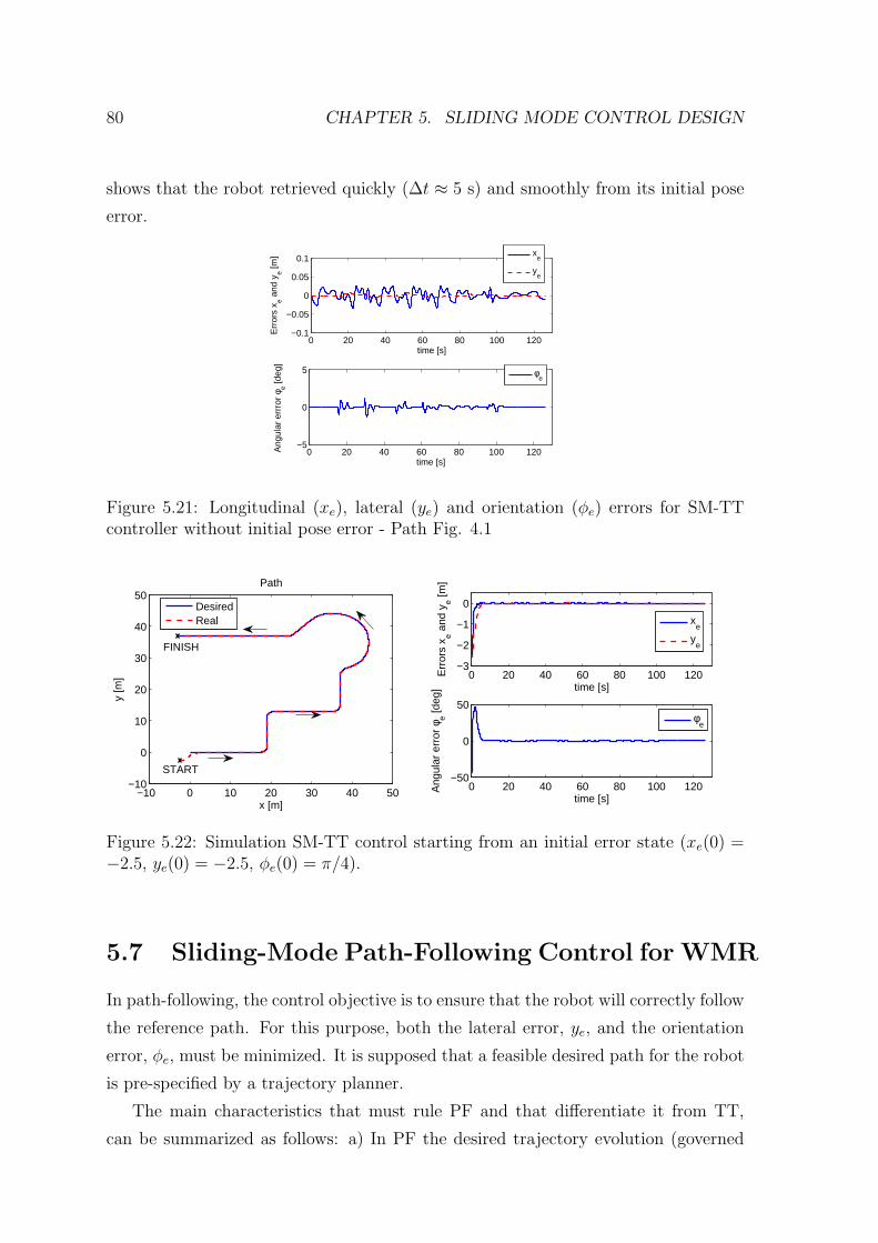
80 CHAPTER 5. SLIDING MODE CONTROL DESIGN
shows that the robot retrieved quickly (∆t ≈ 5 s) and smoothly from its initial pose
error.
0 20 40 60 80 100 120−0.1
−0.05
0
0.05
0.1
time [s]
Err
ors
x e and
ye [m
]
x
e
ye
0 20 40 60 80 100 120−5
0
5
time [s]
Ang
ular
err
ror
φ e [deg
]
φe
Figure 5.21: Longitudinal (xe), lateral (ye) and orientation (φe) errors for SM-TTcontroller without initial pose error - Path Fig. 4.1
−10 0 10 20 30 40 50−10
0
10
20
30
40
50Path
x [m]
y [m
]
DesiredReal
FINISH
START
0 20 40 60 80 100 120−3
−2
−1
0
time [s]
Err
ors
x e and
ye [m
]
xe
ye
0 20 40 60 80 100 120−50
0
50
time [s]
Ang
ular
err
or φ
e [deg
]
φe
Figure 5.22: Simulation SM-TT control starting from an initial error state (xe(0) =−2.5, ye(0) = −2.5, φe(0) = π/4).
5.7 Sliding-Mode Path-Following Control for WMR
In path-following, the control objective is to ensure that the robot will correctly follow
the reference path. For this purpose, both the lateral error, ye, and the orientation
error, φe, must be minimized. It is supposed that a feasible desired path for the robot
is pre-specified by a trajectory planner.
The main characteristics that must rule PF and that differentiate it from TT,
can be summarized as follows: a) In PF the desired trajectory evolution (governed
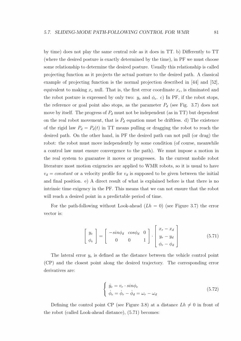
5.7. SLIDING-MODE PATH-FOLLOWING CONTROL FOR WMR 81
by time) does not play the same central role as it does in TT. b) Differently to TT
(where the desired posture is exactly determined by the time), in PF we must choose
some relationship to determine the desired posture. Usually this relationship is called
projecting function as it projects the actual posture to the desired path. A classical
example of projecting function is the normal projection described in [44] and [52],
equivalent to making xe null. That is, the first error coordinate xe, is eliminated and
the robot posture is expressed by only two: ye and φe. c) In PF, if the robot stops,
the reference or goal point also stops, as the parameter Pd (see Fig. 3.7) does not
move by itself. The progress of Pd must not be independent (as in TT) but dependent
on the real robot movement, that is Pd equation must be driftless. d) The existence
of the rigid law Pd = Pd(t) in TT means pulling or dragging the robot to reach the
desired path. On the other hand, in PF the desired path can not pull (or drag) the
robot: the robot must move independently by some condition (of course, meanwhile
a control law must ensure convergence to the path). We must impose a motion in
the real system to guarantee it moves or progresses. In the current mobile robot
literature most motion exigencies are applied to WMR robots, so it is usual to have
vd = constant or a velocity profile for vd is supposed to be given between the initial
and final position. e) A direct result of what is explained before is that there is no
intrinsic time exigency in the PF. This means that we can not ensure that the robot
will reach a desired point in a predictable period of time.
For the path-following without Look-ahead (Lh = 0) (see Figure 3.7) the error
vector is:
ye
φe
=
−sinφd cosφd 0
0 0 1
·
xr − xd
yr − yd
φr − φd
(5.71)
The lateral error ye is defined as the distance between the vehicle control point
(CP) and the closest point along the desired trajectory. The corresponding error
derivatives are:
ye = vr · sinφe
φe = φr − φd = ωr − ωd
(5.72)
Defining the control point CP (see Figure 3.8) at a distance Lh 6= 0 in front of
the robot (called Look-ahead distance), (5.71) becomes:
82 CHAPTER 5. SLIDING MODE CONTROL DESIGN
ye
φe
=
−sinφd cosφd 0
0 0 1
·
xr − xd + Lh · cosφr
yr − yd + Lh · sinφr
φr − φd
and
ye = vr · sinφe + Lh · ωr · cosφe
φe = φr − φd = ωr − ωd
(5.73)
In this thesis it is assumed that |φe| < π/2, which means that the robot orientation
must not be perpendicular to the desired trajectory.
By definition of the orthogonal projection xe and xe, remain equal to zero as the
robot moves. Therefore, from the first equation of (5.54) we have:
vd = vr · cosφe + ωd · ye (5.74)
under the hypothesis that the desired path curvature k = ωd
vdis continuous and
bounded, equation (5.74) can be rewritten as:
vd =
(
cosφe
1− k · ye
)
· vr (5.75)
under the constraint: (1− k · ye) > 0. A velocity profile for vr is supposed to be given
between the initial and final position where vr = 0 (when vr = 0, ωr = 0 as well).
Let us define the sliding surface
s = ye + k2 · ye + k0 · sgn(ye) · φe (5.76)
whose time derivative is:
s = vr · φe · cosφe + k2 · vr · sinφe + k0 · sgn(ye) · φe (5.77)
From (5.34), (5.77) and knowing that
φe = φr − φd = ωr − ωd
one gets the steering command
ωc =−q2 · s− p2 · sgn(s)− k2 · vr · sinφe
vr · cosφe + k0 · sgn(ye)+ ωd (5.78)
5.7. SLIDING-MODE PATH-FOLLOWING CONTROL FOR WMR 83
where
ωd = k ·
(
cosφe
1− k · ye
)
· vr (5.79)
For the case of using look-ahead Lh:
ωc =1
Lh · cosφe
· (−q2 · s− p2 · sgn(s)− k2 · ye−
−vr · φe · cosφe + Lh · φ2e · sinφe − k0sgn(ye) · φe
)
+ ωd
(5.80)
Let us define V = 12· s2 as a Lyapunov function candidate, therefore its time
derivative is
V = s · s
= s · (ye + k2 · ye + k0 · sgn(ye) · φe)
= s · (−q2 · s− p2 · sgn(s))
= −q2 · s2 − p2 ·
s2
|s|
For V to be negative semi-definite, it is sufficient to choose q2 and p2 such that
q2, p2 > 0.
For the longitudinal velocity we may have different situations namely: 1) vc =
constant; 2) vc = vd; 3) vc given by a longitudinal controller, which has as input the
velocity error (vd − vr), and possibly robot acceleration data. In practical applica-
tions, the desired velocity vd needs to be calculated online such that its values are
in accordance to the associated path. This requires that the feedback information of
the pose and velocity of the robot be inputs of the path planner.
5.7.1 Simulation Results
In this subsection, simulation results of the SM-PF proposed controller are presented.
The simulation model block diagram is shown in Fig. 5.23.
Figures 5.24 and 5.27 show the simulation results using SM-PF control in case
of Path presented in Fig. 5.6b. In the first figure is presented the situation when
vc = vd, where vd is equal to linear velocity from Fig. 5.7a and the second show the
case when vc = constant = 0.5 m/s.
In case of SM-PF control only the lateral error, ye, and the orientation error, φe,
must be minimized. From Figs. 5.26 and 5.29 we can observe that the errors (ye and
φe) are maintained around zero.
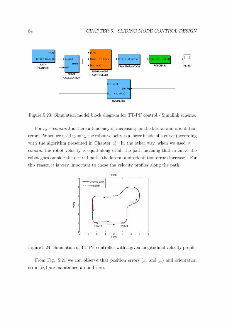
84 CHAPTER 5. SLIDING MODE CONTROL DESIGN
Figure 5.23: Simulation model block diagram for TT-PF control - Simulink scheme.
For vc = constant is there a tendency of increasing for the lateral and orientation
errors. When we used vc = vd the robot velocity is a lower inside of a curve (according
with the algorithm presented in Chapter 4). In the other way, when we used vc =
constat the robot velocity is equal along of all the path meaning that in curve the
robot goes outside the desired path (the lateral and orientation errors increase). For
this reason it is very important to chose the velocity profiles along the path.
−2 −1 0 1 2 3 4 5 6−1
0
1
2
3
4
5
x [m]
y [m
]
Path
Desired path
Real path
START FINISH
Figure 5.24: Simulation of TT-PF controller with a given longitudinal velocity profile.
From Fig. 5.21 we can observe that position errors (xe and ye) and orientation
error (φe) are maintained around zero.
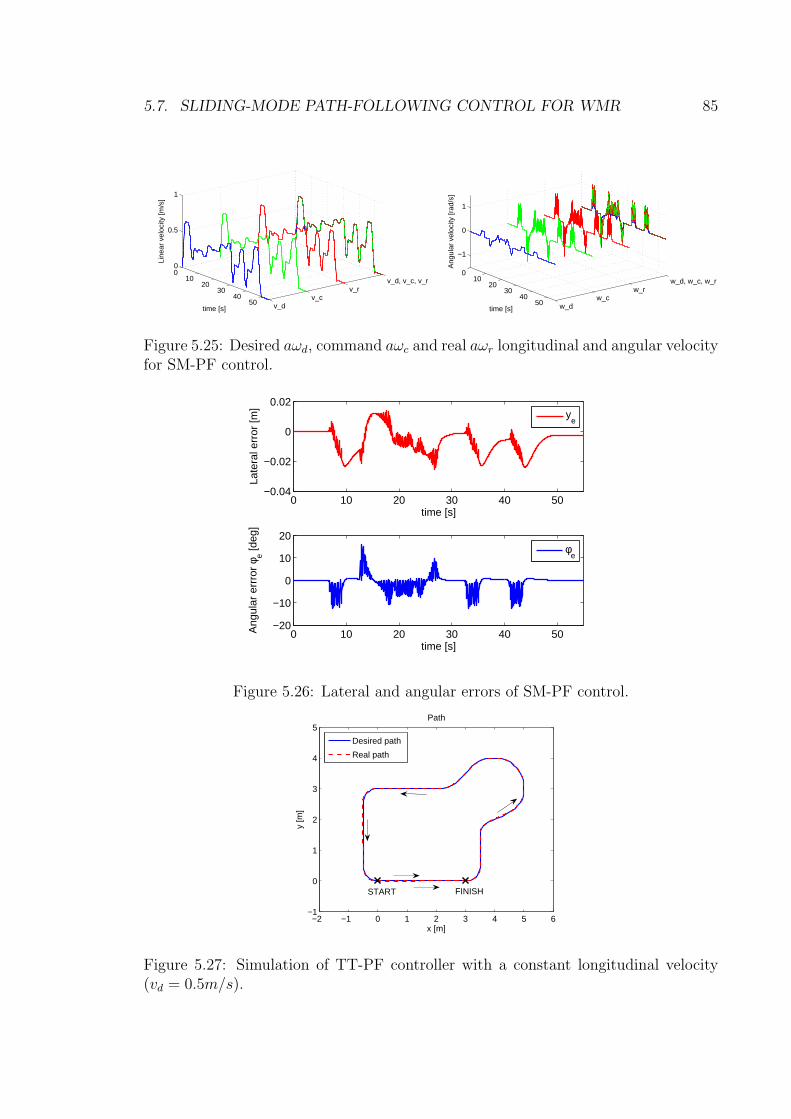
5.7. SLIDING-MODE PATH-FOLLOWING CONTROL FOR WMR 85
v_dv_c
v_rv_d, v_c, v_r
010
2030
4050
0
0.5
1
time [s]
Line
ar v
eloc
ity [m
/s]
w_dw_c
w_rw_d, w_c, w_r
010
2030
4050
−1
0
1
time [s]
Ang
ular
vel
ocity
[rad
/s]
Figure 5.25: Desired aωd, command aωc and real aωr longitudinal and angular velocityfor SM-PF control.
0 10 20 30 40 50−0.04
−0.02
0
0.02
time [s]
Late
ral e
rror
[m]
ye
0 10 20 30 40 50−20
−10
0
10
20
time [s]
Ang
ular
err
ror
φ e [deg
]
φe
Figure 5.26: Lateral and angular errors of SM-PF control.
−2 −1 0 1 2 3 4 5 6−1
0
1
2
3
4
5
x [m]
y [m
]
Path
Desired path
Real path
START FINISH
Figure 5.27: Simulation of TT-PF controller with a constant longitudinal velocity(vd = 0.5m/s).
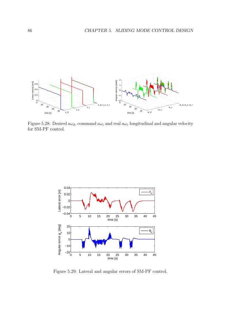
86 CHAPTER 5. SLIDING MODE CONTROL DESIGN
v_dv_c
v_rv_d, v_c, v_r
010
2030
40
0
0.2
0.4
0.6
time [s]
Line
ar v
eloc
ity [m
/s]
w_dw_c
w_rw_d, w_c, w_r
010
2030
40
−2
−1
0
1
2
time [s]
Ang
ular
vel
ocity
[rad
/s]
Figure 5.28: Desired aωd, command aωc and real aωr longitudinal and angular velocityfor SM-PF control.
0 5 10 15 20 25 30 35 40 45−0.04
−0.02
0
0.02
0.04
time [s]
Late
ral e
rror
[m]
ye
0 5 10 15 20 25 30 35 40 45−20
−10
0
10
20
time [s]
Ang
ular
err
ror
φ e [deg
]
φe
Figure 5.29: Lateral and angular errors of SM-PF control.
Chapter 6
Human Body Comfort
6.1 Introduction
Many people nowadays spend a significant proportion of their time travelling and
there is an increasing demand for comfort, in private and public transportation. Three
classes of factors are considered in the analysis of travelling comfort: organizational,
local and riding. The riding comfort can be analysed in three different respects:
dynamic factors - related to vibration, shocks and acceleration; ambient factors -
thermal comfort, air quality, noise, pressure gradients, etc; spatial factors - dealing
with the ergonomics of the passenger’s position.
In today’s aged society, a wheelchair is the most common vehicle to assist elderly
and disabled people. Wheelchairs can provide many profits to users, such as extending
mobility, enlarging community and social activities, and enhancing quality of life of
the users. Therefore, the number of users of electric powered wheelchairs is increasing,
and the development of wheelchairs which are able to drive comfortably is highly
required.
Various factors are largely related to the riding comfort of electric powered wheel-
chairs, such as seat comfort, ambient noise, and stability. The passenger’s posture
swing of body and the driving acceleration and deceleration are generally the main
factors which influence comfort.
In the international standard of ISO-2631-1 [133], the riding comfort of a trans-
portation vehicle is evaluated by the magnitude of the acceleration weighted by os-
cillation frequency.
Passenger’s comfort while riding wheelchairs is also improved by suppressing the
vibration with discomfort frequencies. Maeda [113] described that a wheelchair with
87
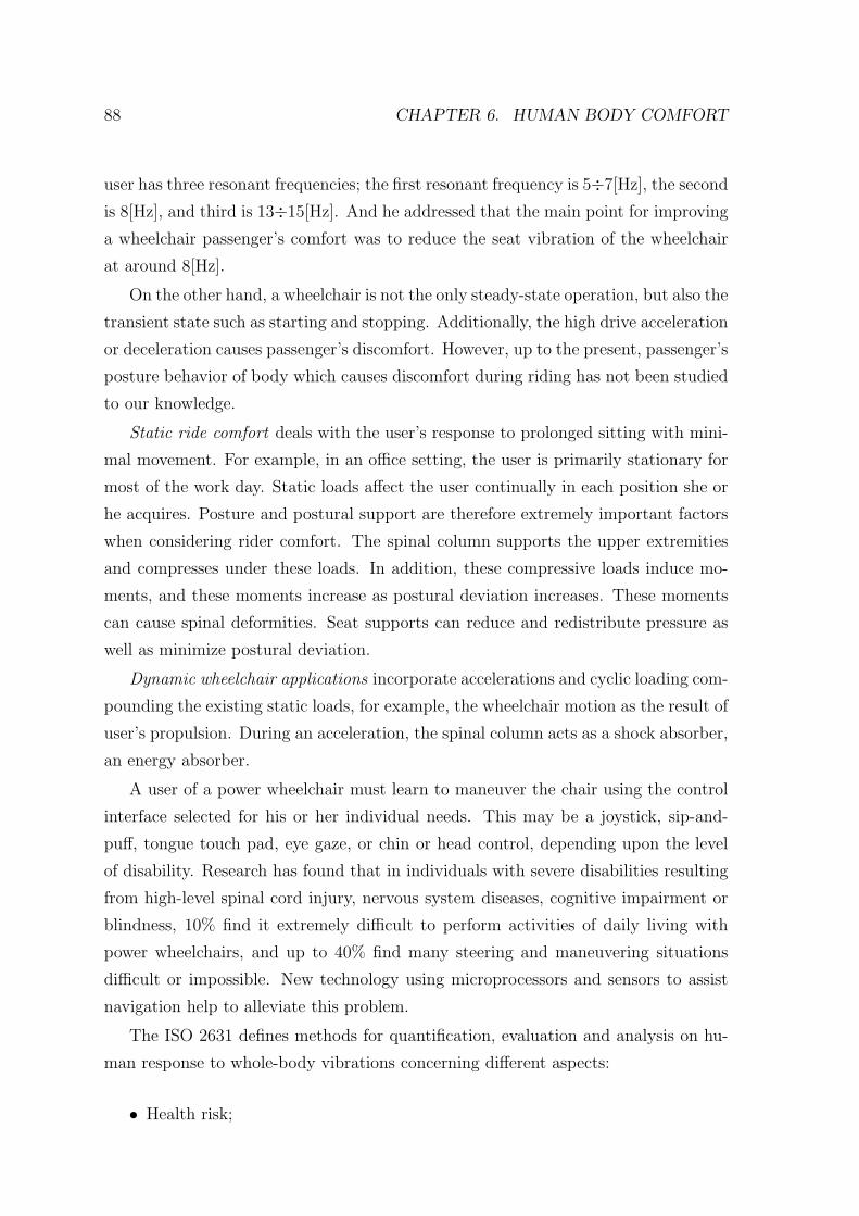
88 CHAPTER 6. HUMAN BODY COMFORT
user has three resonant frequencies; the first resonant frequency is 5÷7[Hz], the second
is 8[Hz], and third is 13÷15[Hz]. And he addressed that the main point for improving
a wheelchair passenger’s comfort was to reduce the seat vibration of the wheelchair
at around 8[Hz].
On the other hand, a wheelchair is not the only steady-state operation, but also the
transient state such as starting and stopping. Additionally, the high drive acceleration
or deceleration causes passenger’s discomfort. However, up to the present, passenger’s
posture behavior of body which causes discomfort during riding has not been studied
to our knowledge.
Static ride comfort deals with the user’s response to prolonged sitting with mini-
mal movement. For example, in an office setting, the user is primarily stationary for
most of the work day. Static loads affect the user continually in each position she or
he acquires. Posture and postural support are therefore extremely important factors
when considering rider comfort. The spinal column supports the upper extremities
and compresses under these loads. In addition, these compressive loads induce mo-
ments, and these moments increase as postural deviation increases. These moments
can cause spinal deformities. Seat supports can reduce and redistribute pressure as
well as minimize postural deviation.
Dynamic wheelchair applications incorporate accelerations and cyclic loading com-
pounding the existing static loads, for example, the wheelchair motion as the result of
user’s propulsion. During an acceleration, the spinal column acts as a shock absorber,
an energy absorber.
A user of a power wheelchair must learn to maneuver the chair using the control
interface selected for his or her individual needs. This may be a joystick, sip-and-
puff, tongue touch pad, eye gaze, or chin or head control, depending upon the level
of disability. Research has found that in individuals with severe disabilities resulting
from high-level spinal cord injury, nervous system diseases, cognitive impairment or
blindness, 10% find it extremely difficult to perform activities of daily living with
power wheelchairs, and up to 40% find many steering and maneuvering situations
difficult or impossible. New technology using microprocessors and sensors to assist
navigation help to alleviate this problem.
The ISO 2631 defines methods for quantification, evaluation and analysis on hu-
man response to whole-body vibrations concerning different aspects:
• Health risk;
6.1. INTRODUCTION 89
• Comfort and perception;
• Motion sickness.
Comfort is a complex definition that contains both physiological and psycholog-
ical components; this includes the subjective feeling of well being with the absence
of discomfort, stress and pain. Comfort not only consists of the absence of negative
effects; it is also the experience of positive aspects of comfort. Therefore, comfort
includes a form of evaluation, i.e. it feels well and has as its opposite, negative
sensations. From interviews of vehicle passengers its obvious that ride comfort is
dependent not only on the magnitude but also on the occurrence of occasional shocks
or transients.
Ride quality is a persons reaction to a set of physical conditions in a vehicle envi-
ronment, such as dynamic, ambient and spatial variables. Dynamic variables consist
of motions, measured as accelerations and changes (jerk) in accelerations in all three
axes (lateral, longitudinal and vertical), angular motions about these axes (roll, pitch
and yaw) and sudden motions, such as shocks and jolts. Normally, the axes are fixed
to the vehicle body. The ambient variables may include temperature, pressure, air
quality and ventilation, as well as noise and high frequency vibrations, while the spa-
tial variables may include workspace, leg room and other seating variables. However,
many use the term passenger comfort, ride comfort or average ride comfort for ratings
on a ride quality scale regarding the influence of dynamic variables. Normally, higher
rating on a ride quality scale means better comfort, whereas higher rating on a ride
(dis-)comfort scale means less comfort.
The human evaluation of comfort, ride quality, involves not only motion quantities
but also human interaction variables (see Figure 6.1).
In the time domain an analysis points out parameters like: peak value, standard
deviation, root mean square value (rms), running rms, crest factor, energy equivalent
rms, estimated Vibration Dose Value (eVDV), root-mean-quad (rmq) or Vibration
Dose Value (VDV). The evaluations and weightings in the frequency domain can be
realized via a Fast Fourier Transformation (FFT) or in the power spectrum. The
most important parameters are summarized in Tabel 6.1
The evaluation of vibration is defined by the specification of the rms value of the
acceleration a in [m/s2] for translational and for rotational vibrations in [rad/s2]:
aq =
[
1
T·∫ T
0a2
q(t)dt
]12
(6.1)
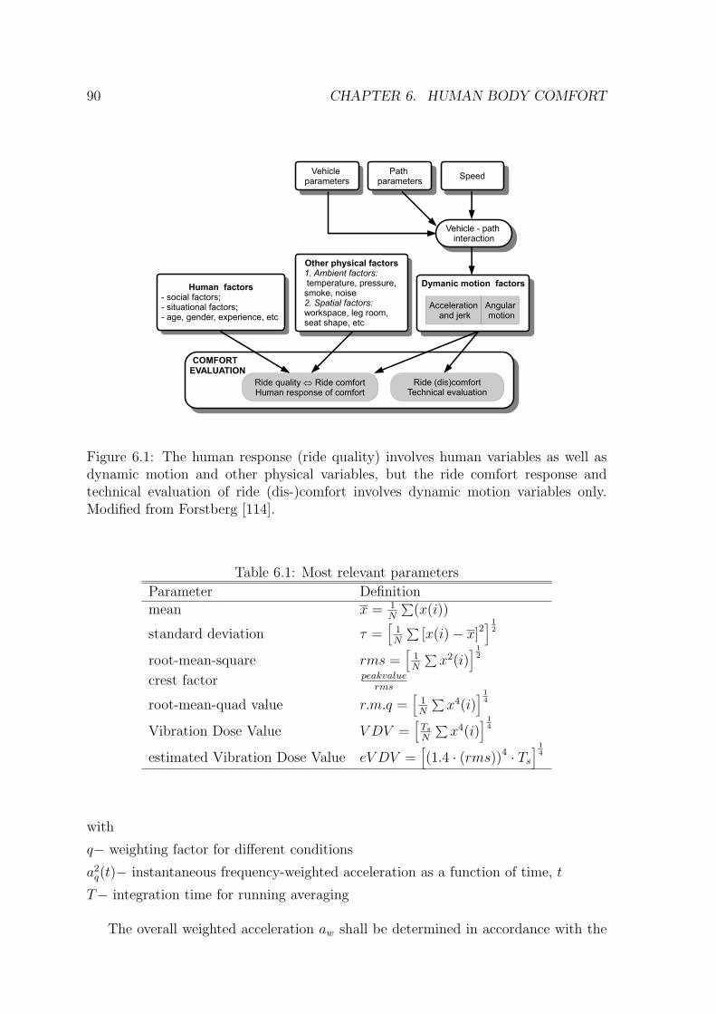
90 CHAPTER 6. HUMAN BODY COMFORT
Figure 6.1: The human response (ride quality) involves human variables as well asdynamic motion and other physical variables, but the ride comfort response andtechnical evaluation of ride (dis-)comfort involves dynamic motion variables only.Modified from Forstberg [114].
Table 6.1: Most relevant parameters
Parameter Definitionmean x = 1
N
∑
(x(i))
standard deviation τ =[
1N
∑
[x(i)− x]2] 1
2
root-mean-square rms =[
1N
∑
x2(i)] 1
2
crest factor peakvaluerms
root-mean-quad value r.m.q =[
1N
∑
x4(i)]
14
Vibration Dose Value V DV =[
Ts
N
∑
x4(i)]
14
estimated Vibration Dose Value eV DV =[
(1.4 · (rms))4 · Ts
]14
with
q− weighting factor for different conditions
a2q(t)− instantaneous frequency-weighted acceleration as a function of time, t
T− integration time for running averaging
The overall weighted acceleration aw shall be determined in accordance with the
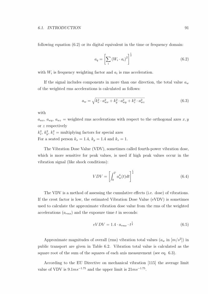
6.1. INTRODUCTION 91
following equation (6.2) or its digital equivalent in the time or frequency domain:
aq =
[
∑
i
(Wi · ai)2
]12
(6.2)
with Wi is frequency weighting factor and ai is rms acceleration.
If the signal includes components in more than one direction, the total value aw
of the weighted rms accelerations is calculated as follows:
aw =√
k2x · a
2wx + k2
y · a2wy + k2
z · a2wz (6.3)
with
awx, awy, awz = weighted rms accelerations with respect to the orthogonal axes x, y
or z respectively
k2x, k
2y, k
2z = multiplying factors for special axes
For a seated person kx = 1.4, ky = 1.4 and kz = 1.
The Vibration Dose Value (VDV), sometimes called fourth-power vibration dose,
which is more sensitive for peak values, is used if high peak values occur in the
vibration signal (like shock conditions):
V DV =
[
∫ T
0a4
w(t)dt
] 14
(6.4)
The VDV is a method of assessing the cumulative effects (i.e. dose) of vibrations.
If the crest factor is low, the estimated Vibration Dose Value (eVDV) is sometimes
used to calculate the approximate vibration dose value from the rms of the weighted
accelerations (arms) and the exposure time t in seconds:
eV DV = 1.4 · arms · t14 (6.5)
Approximate magnitudes of overall (rms) vibration total values (aw in [m/s2]) in
public transport are given in Table 6.2. Vibration total value is calculated as the
square root of the sum of the squares of each axis measurement (see eq. 6.3).
According to the EU Directive on mechanical vibration [115] the average limit
value of VDV is 9.1ms−1.75 and the upper limit is 21ms−1.75.
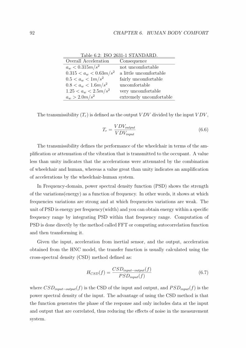
92 CHAPTER 6. HUMAN BODY COMFORT
Table 6.2: ISO 2631-1 STANDARD.Overall Acceleration Consequenceaw < 0.315m/s2 not uncomfortable0.315 < aw < 0.63m/s2 a little uncomfortable0.5 < aw < 1m/s2 fairly uncomfortable0.8 < aw < 1.6m/s2 uncomfortable1.25 < aw < 2.5m/s2 very uncomfortableaw > 2.0m/s2 extremely uncomfortable
The transmissibility (Tr) is defined as the output V DV divided by the input V DV ,
Tr =V DVoutput
V DVinput
(6.6)
The transmissibility defines the performance of the wheelchair in terms of the am-
plification or attenuation of the vibration that is transmitted to the occupant. A value
less than unity indicates that the accelerations were attenuated by the combination
of wheelchair and human, whereas a value great than unity indicates an amplification
of accelerations by the wheelchair-human system.
In Frequency-domain, power spectral density function (PSD) shows the strength
of the variations(energy) as a function of frequency. In other words, it shows at which
frequencies variations are strong and at which frequencies variations are weak. The
unit of PSD is energy per frequency(width) and you can obtain energy within a specific
frequency range by integrating PSD within that frequency range. Computation of
PSD is done directly by the method called FFT or computing autocorrelation function
and then transforming it.
Given the input, acceleration from inertial sensor, and the output, acceleration
obtained from the HNC model, the transfer function is usually calculated using the
cross-spectral density (CSD) method defined as:
HCSD(f) =CSDinput−output(f)
PSDinput(f)(6.7)
where CSDinput−output(f) is the CSD of the input and output, and PSDinput(f) is the
power spectral density of the input. The advantage of using the CSD method is that
the function generates the phase of the response and only includes data at the input
and output that are correlated, thus reducing the effects of noise in the measurement
system.
6.2. MODEL OF HUMAN HEAD-NECK COMPLEX 93
6.2 Model of Human Head-Neck Complex
The human body is a complex dynamic system, the properties of which vary from
moment to moment and from one individual to another. From the results of large
amount of experimental data, various biomechanical models have been developed to
describe the human motion. These models can be grouped as lumped or distributed
parameter models. The lumped parameter models consider the human body as several
rigid bodies, springs and dampers [116], [117], [118]. Some distributed models consider
the spine as a layered structure of rigid elements, representing the vertebral bodies
and deformable elements representing the intervertebral disc by the finite elements
[119].
The dynamic response of seated subjects exposed to vibration has been widely
assessed in terms of the driving point impedance, apparent mass and transmissi-
bility (transmission of motion through the human body). The transmission of the
acceleration to the head-neck complex (HNC) in the seated human body may be the
cause of discomfort and motion sickness in wheelchairs. The seating back, by limiting
the horizontal and rotational motion of the trunk, increases the transmission of the
trunk horizontal acceleration to the HNC. This may has considerable influence on
discomfort.
The present study focuses specifically on the influence of sliding-mode trajectory-
tracking (SM-TT) controller action on user comfort. The user comfort is examined
not only in the time domain (using the transmissibility parameter), but also in the
frequency domain. For measuring accelerations of the wheelchair, a three-dimensional
inertial sensor was used. The analysis of user comfort is made in three different
situations: i) SM-TT control under odometry navigation; ii) when the odometric
data is fused with absolute position data from magnetic markers (using an EKF-based
fusion in the on-line pose estimation); iii) SM-TT control with purposely-incorrectly-
tuned parameters.
A double-inverted pendulum model with two degrees-of-freedom is considered for
the HNC model (Fig. 6.2). One of the centers of rotation of the model was assumed to
be at C7-T1 (O1 in Fig. 6.2), and the other at C0-C1 (O2 in Fig. 6.2) of the cervical
spine. Two lumped masses, indicating the mass of the neck and the mass of the head,
were considered in the model. The center of mass of the neck was assumed to be
exactly at the mid-point of the two centers of rotation. Moreover, the center of mass
of the head was assumed to be exactly over the center of mass of the neck and the
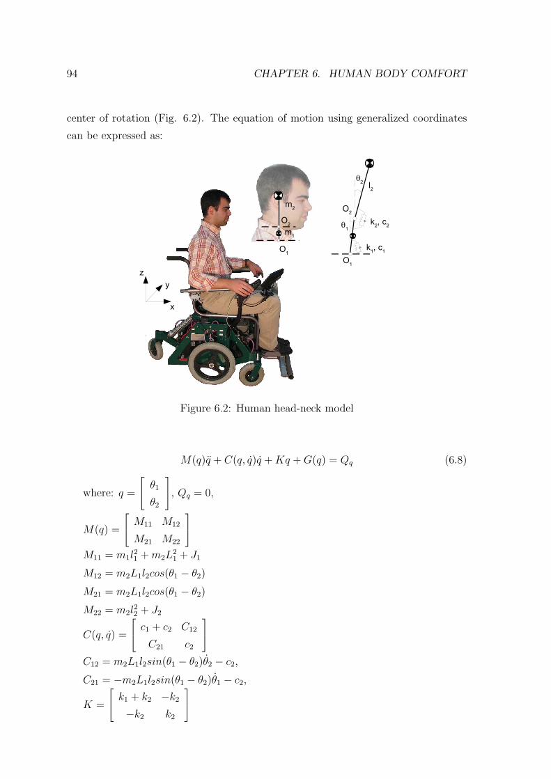
94 CHAPTER 6. HUMAN BODY COMFORT
center of rotation (Fig. 6.2). The equation of motion using generalized coordinates
can be expressed as:
Figure 6.2: Human head-neck model
M(q)q + C(q, q)q +Kq +G(q) = Qq (6.8)
where: q =
θ1
θ2
, Qq = 0,
M(q) =
M11 M12
M21 M22
M11 = m1l21 +m2L
21 + J1
M12 = m2L1l2cos(θ1 − θ2)
M21 = m2L1l2cos(θ1 − θ2)
M22 = m2l22 + J2
C(q, q) =
c1 + c2 C12
C21 c2
C12 = m2L1l2sin(θ1 − θ2)θ2 − c2,
C21 = −m2L1l2sin(θ1 − θ2)θ1 − c2,
K =
k1 + k2 −k2
−k2 k2
6.3. EXPERIMENTAL DATE FROM INERTIAL SENSOR 95
Table 6.3: Characteristics of user’s elementsElement Neck HeadLength of segment Li[m] 0.080 0.138Center of gravity li[m] 0.040 0.069Mass mi[kg] 1.01 4.22Moment of Inertia Ji[kgm
2] 0.0011 0.210Spring constant ki[Nm/rad] 14.04 10.29Damping constant ci[Nms/rad] 0.347 0.230
G(q) =
−(m2L1 +m1l1)xcos(θ1)
−m2l2xcos(θ2)
In my thesis, the user characteristic elements, shown in Table 6.3 (from [116]),
were used to model the dynamic behavior of the human HNC.
6.3 Experimental Date From Inertial Sensor
The analysis of user comfort is made in three different situations:
• case A: SM-TT control under odometry navigation;
• case B: SM-TT control under magnetic-markers navigation (odomeric data is
fused, using an EKF-based fusion, with absolute position data from magnetic
markers detection);
• case C: SM-TT control with purposely-incorrectly-tuned parameters.
The experimental data of all three cases are summarized in Table 6.4. Three ex-
perimental trials were executed in cases A and B. The table shows the vibration
dose value (V DV ), transmissibility (Tr), root mean square accelerations (rms) and
maximum values (Max). The results of columns ”rms accel. Robchair” and ”Max.
accel. RobChair” concern the acceleration results obtained by the inertial sensor;
and the ”rms accel. Head” and ”Max. accel. Head” were obtained from the model
of head-neck complex (6.8). The overall rms acceleration of head (along the x axes)
in cases A and B are in range of ”not uncomfortable”, but in case C is in range of
”uncomfortable” (see Table 6.2 and equation (6.3)).
Each experiment was made for the same trajectory (see Fig. 6.3). The time
domain V DV values obtained in cases A and B are below the limit value of 9.1ms−1.75,
only in case C, V DV values are above that limit. As can be observed from Table
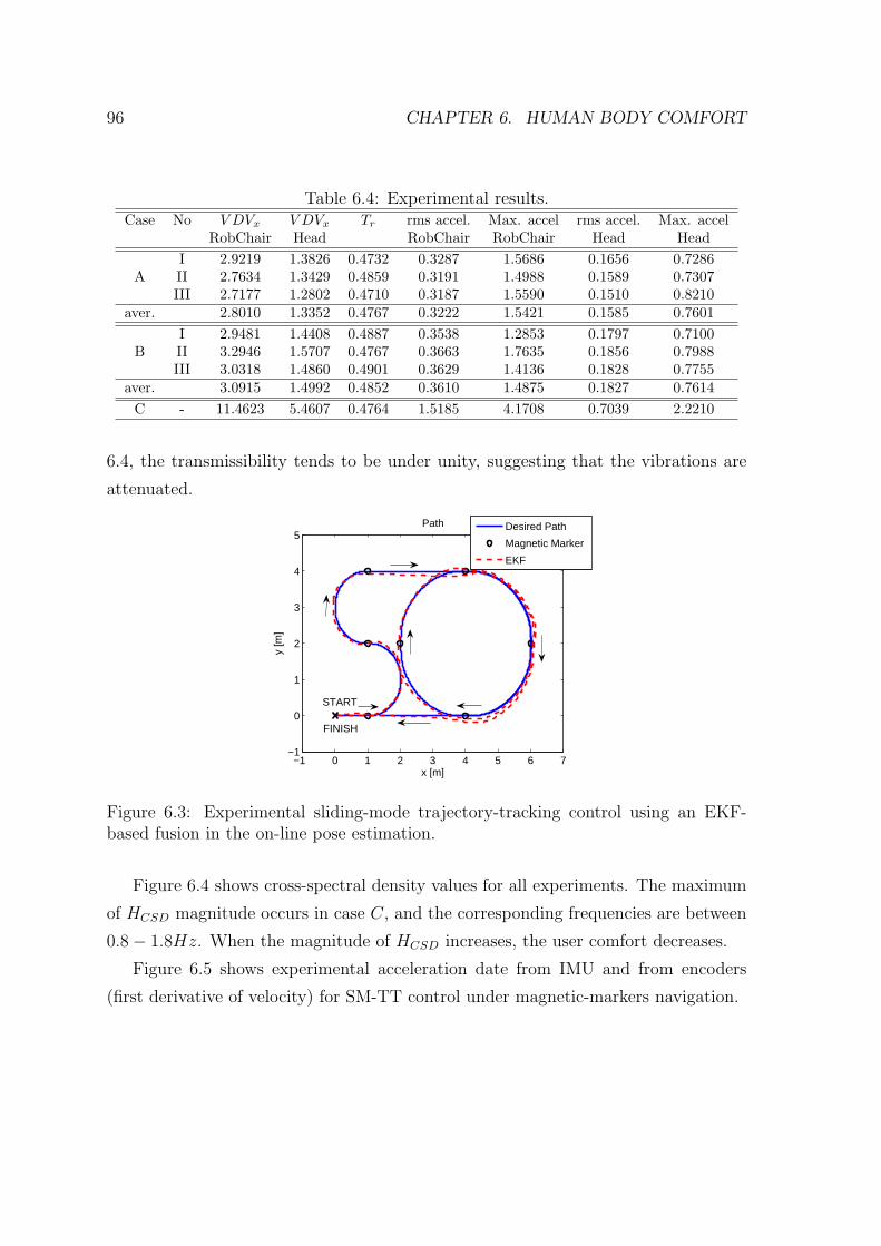
96 CHAPTER 6. HUMAN BODY COMFORT
Table 6.4: Experimental results.Case No V DVx V DVx Tr rms accel. Max. accel rms accel. Max. accel
RobChair Head RobChair RobChair Head Head
I 2.9219 1.3826 0.4732 0.3287 1.5686 0.1656 0.7286A II 2.7634 1.3429 0.4859 0.3191 1.4988 0.1589 0.7307
III 2.7177 1.2802 0.4710 0.3187 1.5590 0.1510 0.8210aver. 2.8010 1.3352 0.4767 0.3222 1.5421 0.1585 0.7601
I 2.9481 1.4408 0.4887 0.3538 1.2853 0.1797 0.7100B II 3.2946 1.5707 0.4767 0.3663 1.7635 0.1856 0.7988
III 3.0318 1.4860 0.4901 0.3629 1.4136 0.1828 0.7755aver. 3.0915 1.4992 0.4852 0.3610 1.4875 0.1827 0.7614
C - 11.4623 5.4607 0.4764 1.5185 4.1708 0.7039 2.2210
6.4, the transmissibility tends to be under unity, suggesting that the vibrations are
attenuated.
−1 0 1 2 3 4 5 6 7−1
0
1
2
3
4
5
x [m]
y [m
]
Path
Desired Path
Magnetic Marker
EKF
FINISH
START
Figure 6.3: Experimental sliding-mode trajectory-tracking control using an EKF-based fusion in the on-line pose estimation.
Figure 6.4 shows cross-spectral density values for all experiments. The maximum
of HCSD magnitude occurs in case C, and the corresponding frequencies are between
0.8− 1.8Hz. When the magnitude of HCSD increases, the user comfort decreases.
Figure 6.5 shows experimental acceleration date from IMU and from encoders
(first derivative of velocity) for SM-TT control under magnetic-markers navigation.
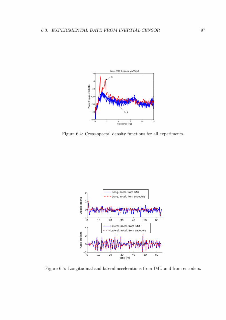
6.3. EXPERIMENTAL DATE FROM INERTIAL SENSOR 97
0 2 4 6 8 10−50
−40
−30
−20
−10
0
10
Frequency (Hz)
Pow
er/fr
eque
ncy
(dB
/Hz)
Cross PSD Estimate via Welch
C
A, B
Figure 6.4: Cross-spectal density functions for all experiments.
0 10 20 30 40 50 60−1
0
1
2
Acc
eler
atio
ns
Long. accel. from IMU
Long. accel. from encoders
0 10 20 30 40 50 60−2
0
2
4
time [m]
Acc
eler
atio
ns
Lateral. accel. from IMU
Lateral. accel. from encoders
Figure 6.5: Longitudinal and lateral accelerations from IMU and from encoders.

98 CHAPTER 6. HUMAN BODY COMFORT
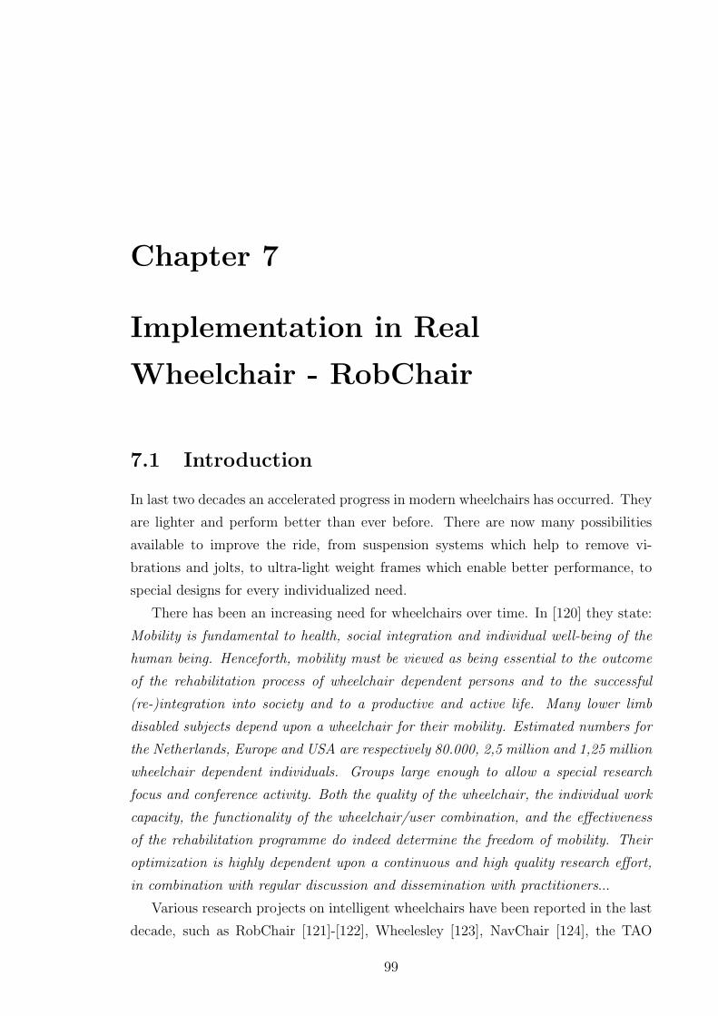
Chapter 7
Implementation in Real
Wheelchair - RobChair
7.1 Introduction
In last two decades an accelerated progress in modern wheelchairs has occurred. They
are lighter and perform better than ever before. There are now many possibilities
available to improve the ride, from suspension systems which help to remove vi-
brations and jolts, to ultra-light weight frames which enable better performance, to
special designs for every individualized need.
There has been an increasing need for wheelchairs over time. In [120] they state:
Mobility is fundamental to health, social integration and individual well-being of the
human being. Henceforth, mobility must be viewed as being essential to the outcome
of the rehabilitation process of wheelchair dependent persons and to the successful
(re-)integration into society and to a productive and active life. Many lower limb
disabled subjects depend upon a wheelchair for their mobility. Estimated numbers for
the Netherlands, Europe and USA are respectively 80.000, 2,5 million and 1,25 million
wheelchair dependent individuals. Groups large enough to allow a special research
focus and conference activity. Both the quality of the wheelchair, the individual work
capacity, the functionality of the wheelchair/user combination, and the effectiveness
of the rehabilitation programme do indeed determine the freedom of mobility. Their
optimization is highly dependent upon a continuous and high quality research effort,
in combination with regular discussion and dissemination with practitioners...
Various research projects on intelligent wheelchairs have been reported in the last
decade, such as RobChair [121]-[122], Wheelesley [123], NavChair [124], the TAO
99
100 CHAPTER 7. IMPLEMENTATION IN REAL WHEELCHAIR - ROBCHAIR
projects [125], SIAMO [126], Rolland [127]-[128], MAid [129]. However, all of these
projects only represent the outgrowths of mobile robot research and few have made
the transition to a commercial product.
The majority of research projects developing intelligent wheelchair sensors, control
and technology have concentrated upon improving the autonomous function of the
mobility aid.
A key task is to provide controls and control modes so that disabled users can
make the most efficient use of their skills and abilities. Techniques developed in
the field of robotics have the potential to offer independent mobility to people who
cannot operate existing controls, and also to reduce the need to tailor these relatively
complex controls and control modes precisely to maximise the user’s skills.
Intelligent wheelchair systems have to be developed under a different set of goals
from other mobile robots. Safety is a key factor for a wheelchair whose task is to
carry a human user. In addition, the wheelchair’s motion must be smooth, so that
the user would feel safe, and comfortable. As the wheelchair operates in a dynamic
environment, the path guidance should also be able to deal with unexpected events
such as dangers or unexpected obstacles on the path.
The intelligent wheelchair, RobChair system, is being developed to overcome
above mentioned problems, allowing the end-user to just perform safe movements
and accomplish some daily life important tasks. The RobChair is a highly interactive
system which is jointly controlled by the human operator and the software of the
robot.
A robotic wheelchair must interact with its user, and for a human-machine sym-
biosis shared control capabilities is required.
The wheelchair must be able to accept inputs from its user not only at the start of
the trip, but throughout the journey. Our wheelchair system will be able to navigate
in indoor and outdoor environments respecting human comfort.
Little is known about how dynamic acceleration affects wheelchair-ride comfort.
Most current literature focuses on the vibration exposure of a seated occupant [130,
131, 132]. Some standards have been developed by the International Organization
for Standardization (ISO) to quantify how much exposure is allowable for various
frequencies of exposure [133]. Although the exposure to whole-body vibration has
been shown to be injurious to seated humans, the effects of wheelchairs and seating
systems on the transmission of vibration to an individual have not been thoroughly
examined.
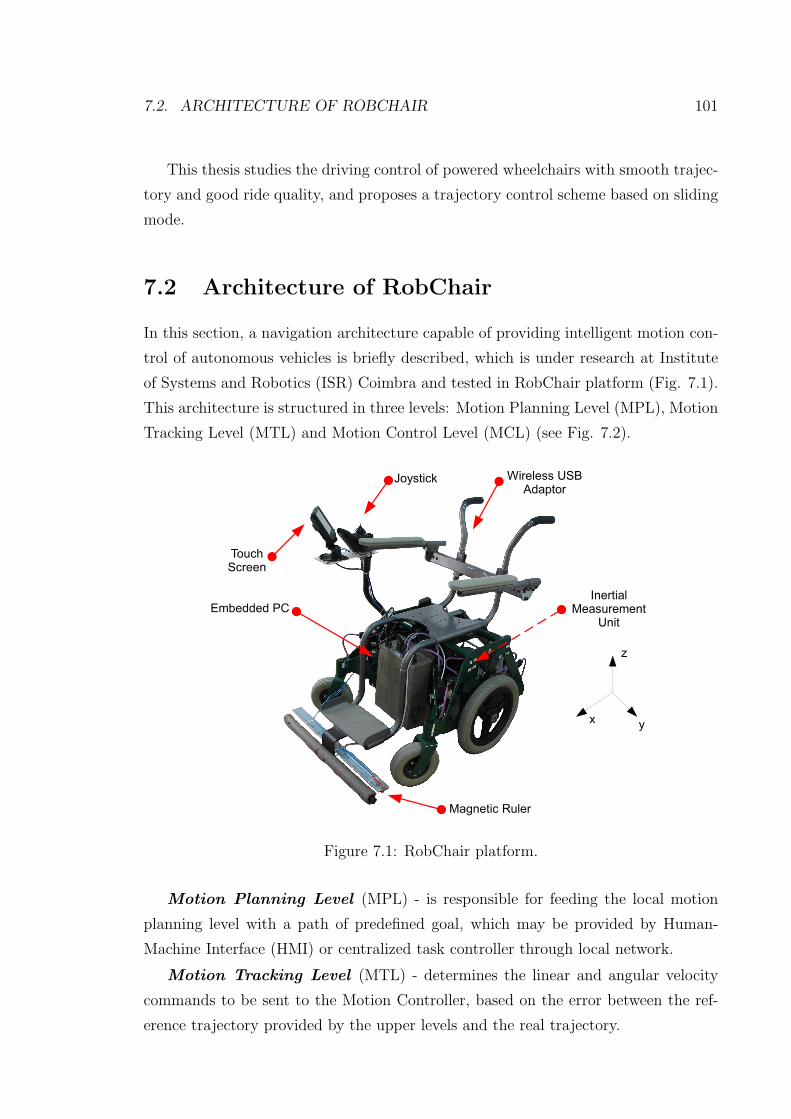
7.2. ARCHITECTURE OF ROBCHAIR 101
This thesis studies the driving control of powered wheelchairs with smooth trajec-
tory and good ride quality, and proposes a trajectory control scheme based on sliding
mode.
7.2 Architecture of RobChair
In this section, a navigation architecture capable of providing intelligent motion con-
trol of autonomous vehicles is briefly described, which is under research at Institute
of Systems and Robotics (ISR) Coimbra and tested in RobChair platform (Fig. 7.1).
This architecture is structured in three levels: Motion Planning Level (MPL), Motion
Tracking Level (MTL) and Motion Control Level (MCL) (see Fig. 7.2).
Figure 7.1: RobChair platform.
Motion Planning Level (MPL) - is responsible for feeding the local motion
planning level with a path of predefined goal, which may be provided by Human-
Machine Interface (HMI) or centralized task controller through local network.
Motion Tracking Level (MTL) - determines the linear and angular velocity
commands to be sent to the Motion Controller, based on the error between the ref-
erence trajectory provided by the upper levels and the real trajectory.
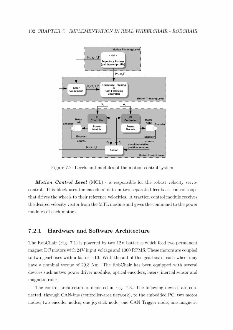
102 CHAPTER 7. IMPLEMENTATION IN REAL WHEELCHAIR - ROBCHAIR
Figure 7.2: Levels and modules of the motion control system.
Motion Control Level (MCL) - is responsible for the robust velocity servo-
control. This block uses the encoders’ data in two separated feedback control loops
that drives the wheels to their reference velocities. A traction control module receives
the desired velocity vector from the MTL module and gives the command to the power
modules of each motors.
7.2.1 Hardware and Software Architecture
The RobChair (Fig. 7.1) is powered by two 12V batteries which feed two permanent
magnet DC motors with 24V input voltage and 1000 RPMS. These motors are coupled
to two gearboxes with a factor 1:10. With the aid of this gearboxes, each wheel may
have a nominal torque of 29,3 Nm. The RobChair has been equipped with several
devices such as two power driver modules, optical encoders, lasers, inertial sensor and
magnetic ruler.
The control architecture is depicted in Fig. 7.3. The following devices are con-
nected, through CAN-bus (controller-area network), to the embedded PC: two motor
nodes; two encoder nodes; one joystick node; one CAN Trigger node; one magnetic
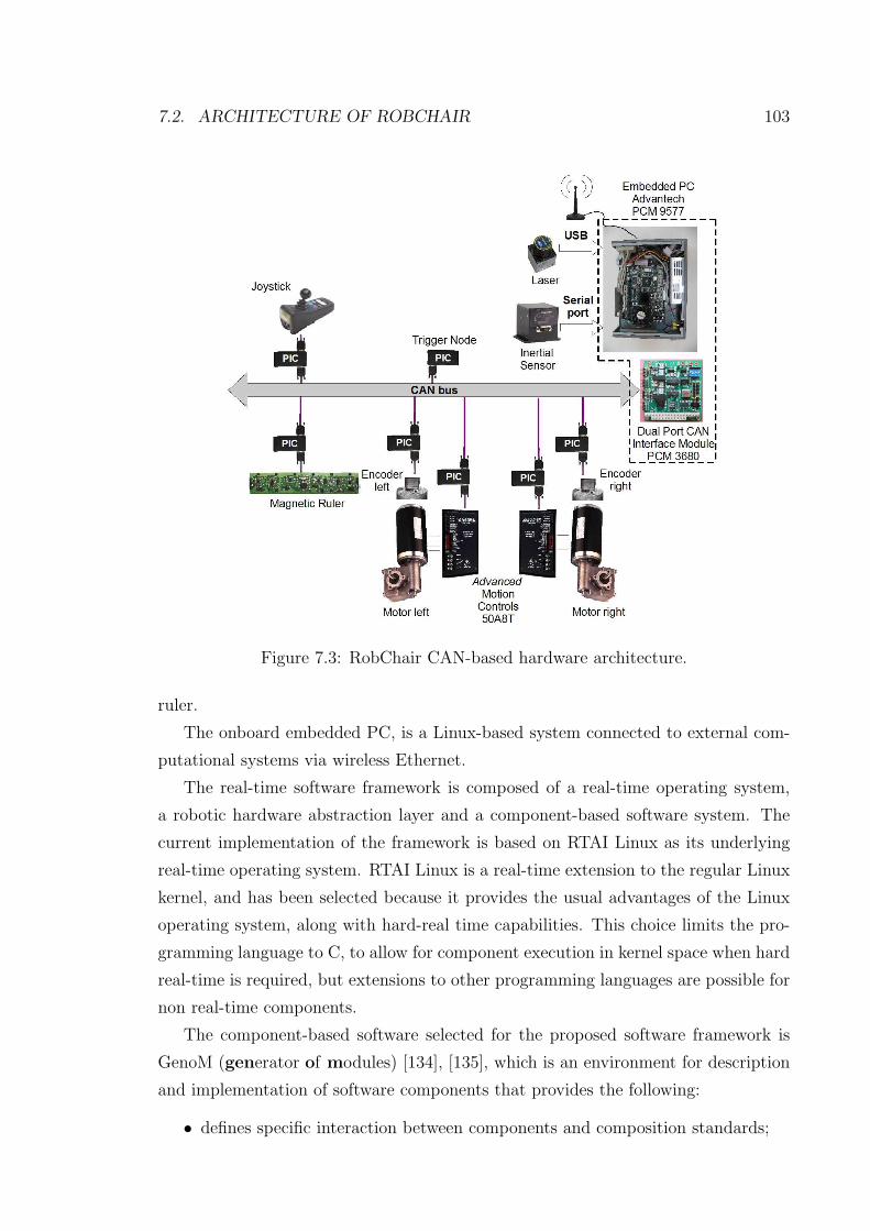
7.2. ARCHITECTURE OF ROBCHAIR 103
Figure 7.3: RobChair CAN-based hardware architecture.
ruler.
The onboard embedded PC, is a Linux-based system connected to external com-
putational systems via wireless Ethernet.
The real-time software framework is composed of a real-time operating system,
a robotic hardware abstraction layer and a component-based software system. The
current implementation of the framework is based on RTAI Linux as its underlying
real-time operating system. RTAI Linux is a real-time extension to the regular Linux
kernel, and has been selected because it provides the usual advantages of the Linux
operating system, along with hard-real time capabilities. This choice limits the pro-
gramming language to C, to allow for component execution in kernel space when hard
real-time is required, but extensions to other programming languages are possible for
non real-time components.
The component-based software selected for the proposed software framework is
GenoM (generator of modules) [134], [135], which is an environment for description
and implementation of software components that provides the following:
• defines specific interaction between components and composition standards;
104 CHAPTER 7. IMPLEMENTATION IN REAL WHEELCHAIR - ROBCHAIR
• provides the dedicated set of executable software elements required to support
the execution of software components that conform to the model;
• defines the internal architecture of software components, and their structure
and functioning;
• provides a set of tools for describing software components and for generating
templates.
As depicted in Fig. 7.3, the CAN fieldbus is used to link the central unit with sev-
eral implemented nodes. The communication is done by a home defined protocol with
which the communication events are synchronized by a trigger (called CAN-trigger).
At every 5 ms, the CAN-trigger sends a command message allowing the other con-
trollers to perform syncronized data acquisition and actuation. The control loop time
of the high-level algorithms that are running in the embedded PC is different from
the low-level control loop. Currently it is settled at 50 ms. Each motor has its own
dedicated controller that performs encoder data acquisition, odometry computation,
and wheel velocity control.
The RobChair is equipped with a magnetic sensing ruler (MSR) developed at
ISR-UC that is able to perform a robust detection of magnetic markers [136]. The
experimental results with RobChair primarily show that the detection system is ro-
bust, since it is able to detect true magnetic markers, and to eliminate noisy magnetic
distortions and false markers.
The odometric data calculated based on the wheel encoders is fused with the data
from magnetic markers. The extended Kalman filter (EKF) was chosen for the fusion
process, as summarized in Table 7.1. The robot pose defined by the Cartesian coordi-
nates (xr, yr) and heading (φr) are the state variables of the EKF. The magnetic ruler
measures are treated as measurements in the fusion process. For a detailed descrip-
tion of the fusion algorithm see [136]. This navigation technology, based on sensing
magnetic markers, is well suited when high precision navigation and robustness is
required, and it can be used to complement other navigation systems, such as GPS.
The inertial sensor RGA300CA-100 (Crossbow) was used for measuring the wheel-
chair accelerations in three orthogonal directions.
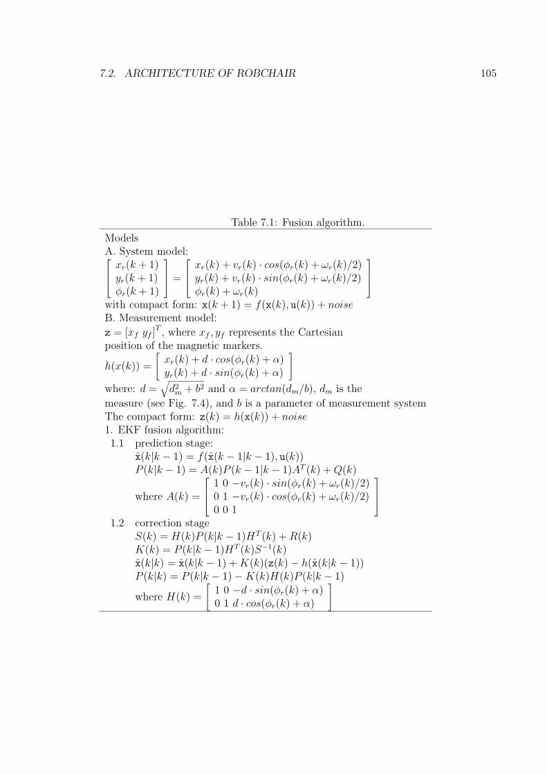
7.2. ARCHITECTURE OF ROBCHAIR 105
Table 7.1: Fusion algorithm.
ModelsA. System model:
xr(k + 1)yr(k + 1)φr(k + 1)
=
xr(k) + vr(k) · cos(φr(k) + ωr(k)/2)yr(k) + vr(k) · sin(φr(k) + ωr(k)/2)φr(k) + ωr(k)
with compact form: x(k + 1) = f(x(k), u(k)) + noiseB. Measurement model:
z = [xf yf ]T , where xf , yf represents the Cartesian
position of the magnetic markers.
h(x(k)) =
[
xr(k) + d · cos(φr(k) + α)yr(k) + d · sin(φr(k) + α)
]
where: d =√
d2m + b2 and α = arctan(dm/b), dm is the
measure (see Fig. 7.4), and b is a parameter of measurement systemThe compact form: z(k) = h(x(k)) + noise1. EKF fusion algorithm:1.1 prediction stage:
x(k|k − 1) = f(x(k − 1|k − 1), u(k))P (k|k − 1) = A(k)P (k − 1|k − 1)AT (k) +Q(k)
where A(k) =
1 0 −vr(k) · sin(φr(k) + ωr(k)/2)0 1 −vr(k) · cos(φr(k) + ωr(k)/2)0 0 1
1.2 correction stageS(k) = H(k)P (k|k − 1)HT (k) +R(k)K(k) = P (k|k − 1)HT (k)S−1(k)x(k|k) = x(k|k − 1) +K(k)(z(k)− h(x(k|k − 1))P (k|k) = P (k|k − 1)−K(k)H(k)P (k|k − 1)
where H(k) =
[
1 0 −d · sin(φr(k) + α)0 1 d · cos(φr(k) + α)
]
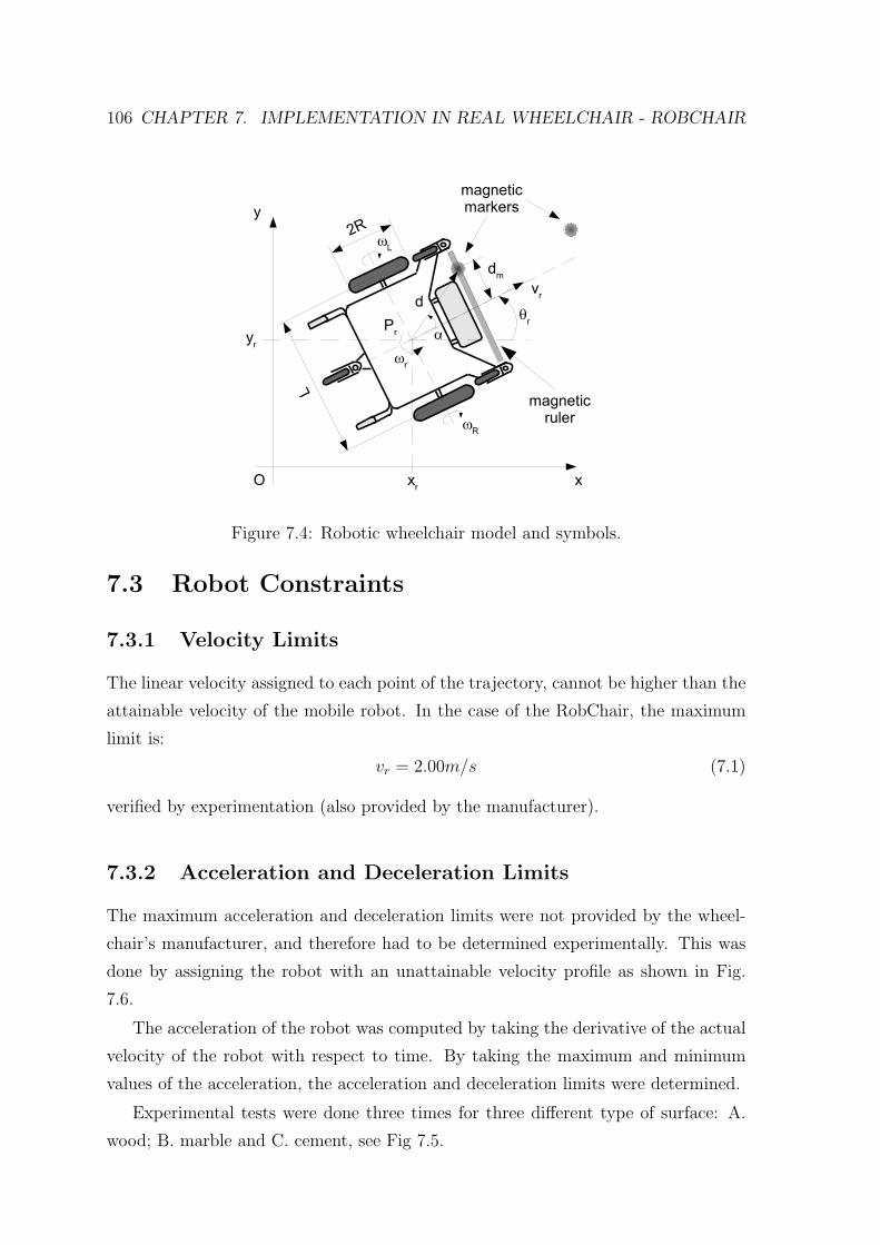
106 CHAPTER 7. IMPLEMENTATION IN REAL WHEELCHAIR - ROBCHAIR
Figure 7.4: Robotic wheelchair model and symbols.
7.3 Robot Constraints
7.3.1 Velocity Limits
The linear velocity assigned to each point of the trajectory, cannot be higher than the
attainable velocity of the mobile robot. In the case of the RobChair, the maximum
limit is:
vr = 2.00m/s (7.1)
verified by experimentation (also provided by the manufacturer).
7.3.2 Acceleration and Deceleration Limits
The maximum acceleration and deceleration limits were not provided by the wheel-
chair’s manufacturer, and therefore had to be determined experimentally. This was
done by assigning the robot with an unattainable velocity profile as shown in Fig.
7.6.
The acceleration of the robot was computed by taking the derivative of the actual
velocity of the robot with respect to time. By taking the maximum and minimum
values of the acceleration, the acceleration and deceleration limits were determined.
Experimental tests were done three times for three different type of surface: A.
wood; B. marble and C. cement, see Fig 7.5.
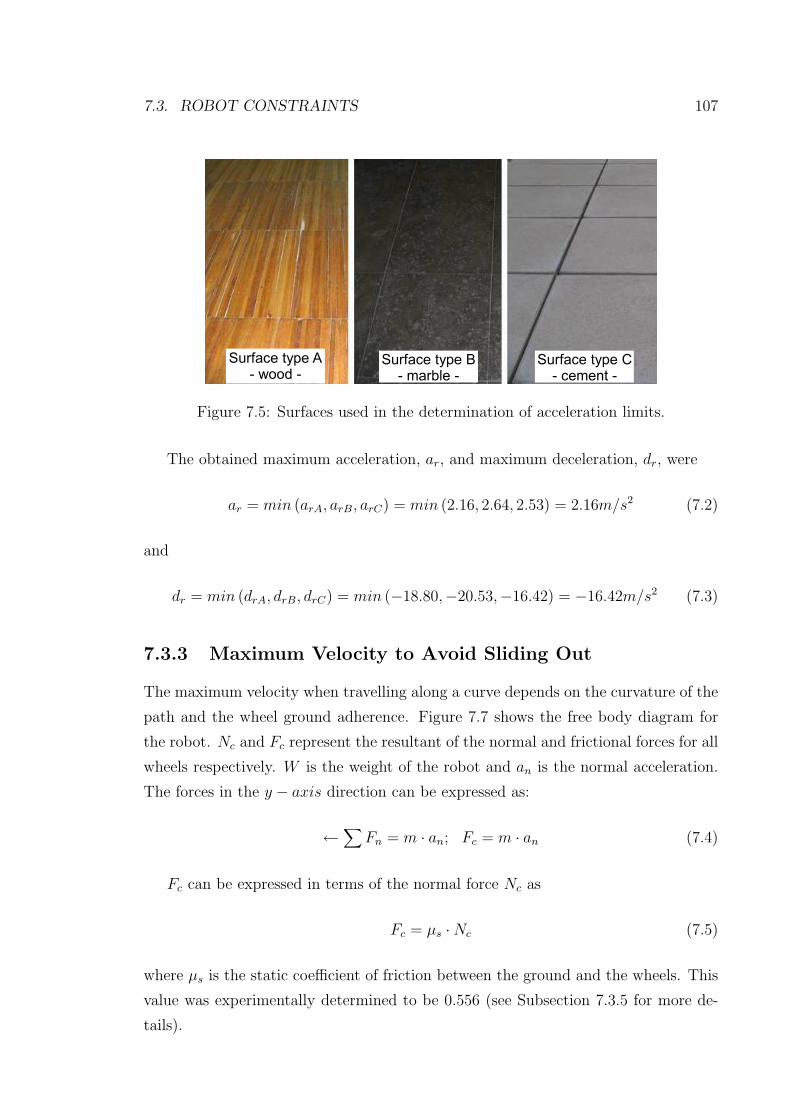
7.3. ROBOT CONSTRAINTS 107
Figure 7.5: Surfaces used in the determination of acceleration limits.
The obtained maximum acceleration, ar, and maximum deceleration, dr, were
ar = min (arA, arB, arC) = min (2.16, 2.64, 2.53) = 2.16m/s2 (7.2)
and
dr = min (drA, drB, drC) = min (−18.80,−20.53,−16.42) = −16.42m/s2 (7.3)
7.3.3 Maximum Velocity to Avoid Sliding Out
The maximum velocity when travelling along a curve depends on the curvature of the
path and the wheel ground adherence. Figure 7.7 shows the free body diagram for
the robot. Nc and Fc represent the resultant of the normal and frictional forces for all
wheels respectively. W is the weight of the robot and an is the normal acceleration.
The forces in the y − axis direction can be expressed as:
←∑
Fn = m · an; Fc = m · an (7.4)
Fc can be expressed in terms of the normal force Nc as
Fc = µs ·Nc (7.5)
where µs is the static coefficient of friction between the ground and the wheels. This
value was experimentally determined to be 0.556 (see Subsection 7.3.5 for more de-
tails).
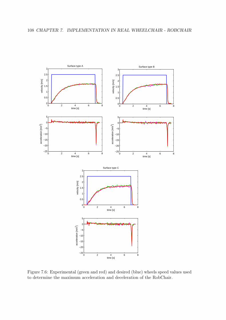
108 CHAPTER 7. IMPLEMENTATION IN REAL WHEELCHAIR - ROBCHAIR
0 2 4 6 80
0.5
1
1.5
2
2.5
3
time [s]
velo
city
[m/s
]
Surface type A
0 2 4 6 8−25
−20
−15
−10
−5
0
5
time [s]
acce
lera
tion
[m/s
2 ]
0 2 4 6 80
0.5
1
1.5
2
2.5
3
time [s]
velo
city
[m/s
]
Surface type B
0 2 4 6 8−25
−20
−15
−10
−5
0
5
time [s]
acce
lera
tion
[m/s
2 ]
0 2 4 6 80
0.5
1
1.5
2
2.5
3
time [s]
velo
city
[m/s
]
Surface type C
0 2 4 6 8−25
−20
−15
−10
−5
0
5
time [s]
acce
lera
tion
[m/s
2 ]
Figure 7.6: Experimental (green and red) and desired (blue) wheels speed values usedto determine the maximum acceleration and deceleration of the RobChair.
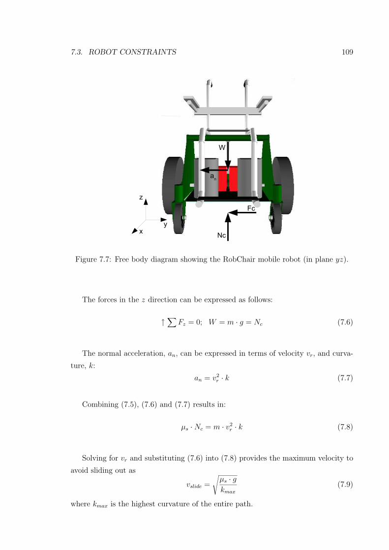
7.3. ROBOT CONSTRAINTS 109
Figure 7.7: Free body diagram showing the RobChair mobile robot (in plane yz).
The forces in the z direction can be expressed as follows:
↑∑
Fz = 0; W = m · g = Nc (7.6)
The normal acceleration, an, can be expressed in terms of velocity vr, and curva-
ture, k:
an = v2r · k (7.7)
Combining (7.5), (7.6) and (7.7) results in:
µs ·Nc = m · v2r · k (7.8)
Solving for vr and substituting (7.6) into (7.8) provides the maximum velocity to
avoid sliding out as
vslide =
√
µs · g
kmax
(7.9)
where kmax is the highest curvature of the entire path.
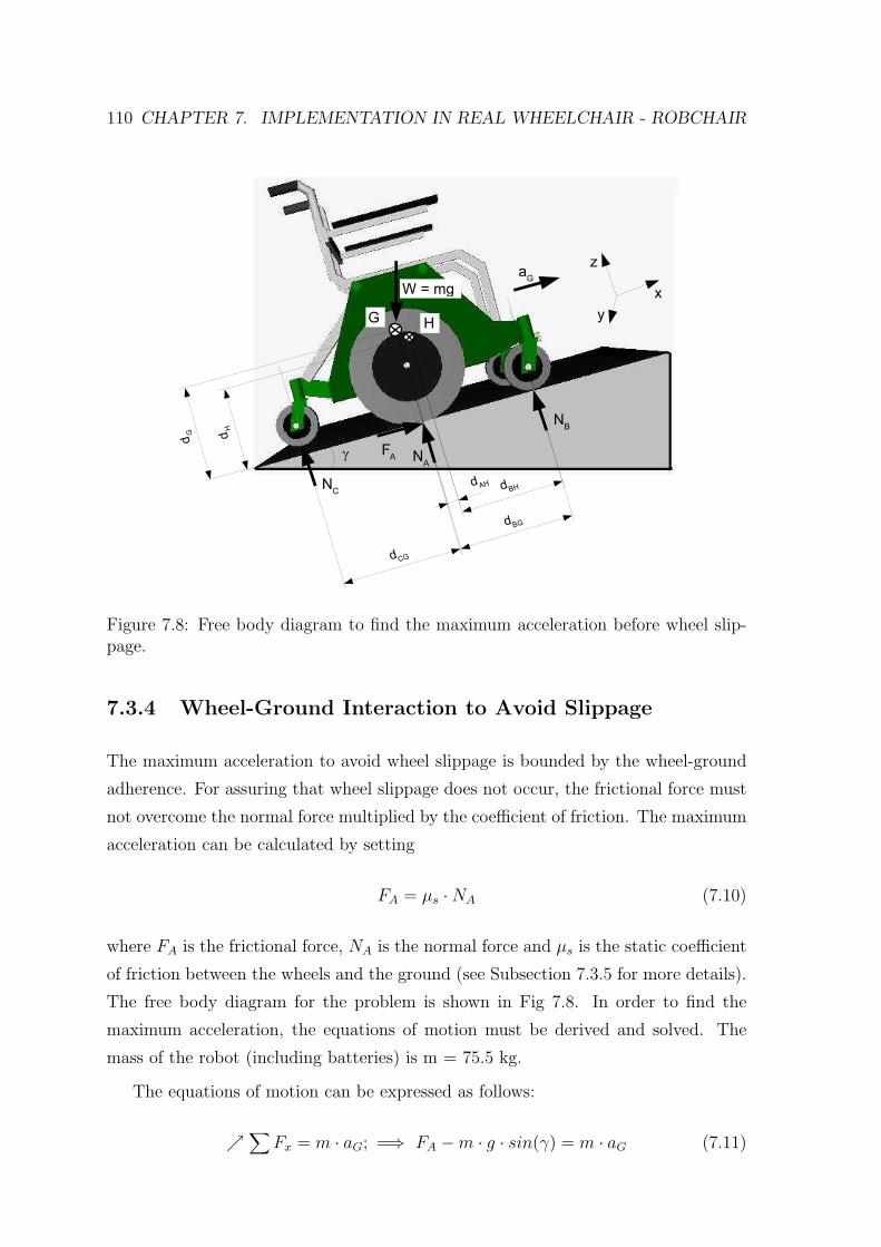
110 CHAPTER 7. IMPLEMENTATION IN REAL WHEELCHAIR - ROBCHAIR
Figure 7.8: Free body diagram to find the maximum acceleration before wheel slip-page.
7.3.4 Wheel-Ground Interaction to Avoid Slippage
The maximum acceleration to avoid wheel slippage is bounded by the wheel-ground
adherence. For assuring that wheel slippage does not occur, the frictional force must
not overcome the normal force multiplied by the coefficient of friction. The maximum
acceleration can be calculated by setting
FA = µs ·NA (7.10)
where FA is the frictional force, NA is the normal force and µs is the static coefficient
of friction between the wheels and the ground (see Subsection 7.3.5 for more details).
The free body diagram for the problem is shown in Fig 7.8. In order to find the
maximum acceleration, the equations of motion must be derived and solved. The
mass of the robot (including batteries) is m = 75.5 kg.
The equations of motion can be expressed as follows:
ր∑
Fx = m · aG; =⇒ FA −m · g · sin(γ) = m · aG (7.11)
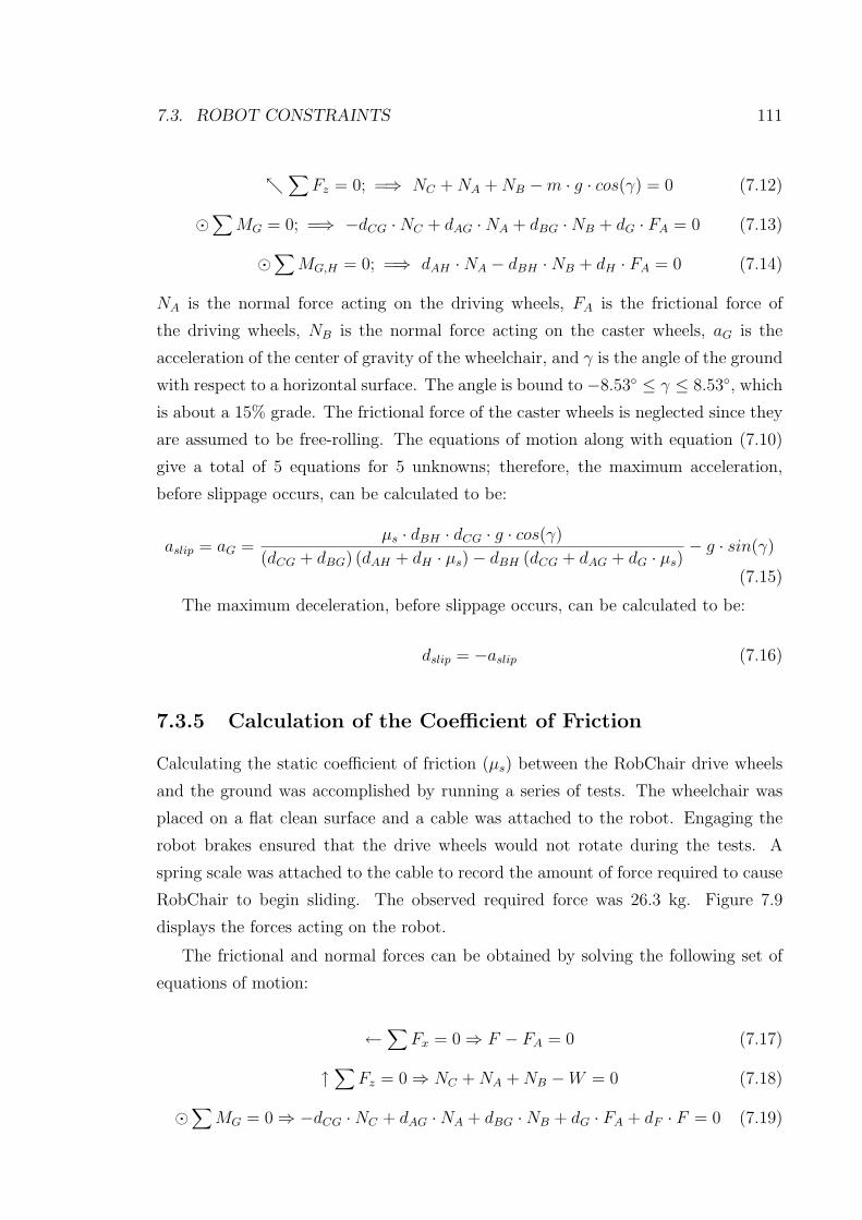
7.3. ROBOT CONSTRAINTS 111
տ∑
Fz = 0; =⇒ NC +NA +NB −m · g · cos(γ) = 0 (7.12)
⊙∑
MG = 0; =⇒ −dCG ·NC + dAG ·NA + dBG ·NB + dG · FA = 0 (7.13)
⊙∑
MG,H = 0; =⇒ dAH ·NA − dBH ·NB + dH · FA = 0 (7.14)
NA is the normal force acting on the driving wheels, FA is the frictional force of
the driving wheels, NB is the normal force acting on the caster wheels, aG is the
acceleration of the center of gravity of the wheelchair, and γ is the angle of the ground
with respect to a horizontal surface. The angle is bound to −8.53 ≤ γ ≤ 8.53, which
is about a 15% grade. The frictional force of the caster wheels is neglected since they
are assumed to be free-rolling. The equations of motion along with equation (7.10)
give a total of 5 equations for 5 unknowns; therefore, the maximum acceleration,
before slippage occurs, can be calculated to be:
aslip = aG =µs · dBH · dCG · g · cos(γ)
(dCG + dBG) (dAH + dH · µs)− dBH (dCG + dAG + dG · µs)− g · sin(γ)
(7.15)
The maximum deceleration, before slippage occurs, can be calculated to be:
dslip = −aslip (7.16)
7.3.5 Calculation of the Coefficient of Friction
Calculating the static coefficient of friction (µs) between the RobChair drive wheels
and the ground was accomplished by running a series of tests. The wheelchair was
placed on a flat clean surface and a cable was attached to the robot. Engaging the
robot brakes ensured that the drive wheels would not rotate during the tests. A
spring scale was attached to the cable to record the amount of force required to cause
RobChair to begin sliding. The observed required force was 26.3 kg. Figure 7.9
displays the forces acting on the robot.
The frictional and normal forces can be obtained by solving the following set of
equations of motion:
←∑
Fx = 0⇒ F − FA = 0 (7.17)
↑∑
Fz = 0⇒ NC +NA +NB −W = 0 (7.18)
⊙∑
MG = 0⇒ −dCG ·NC + dAG ·NA + dBG ·NB + dG · FA + dF · F = 0 (7.19)
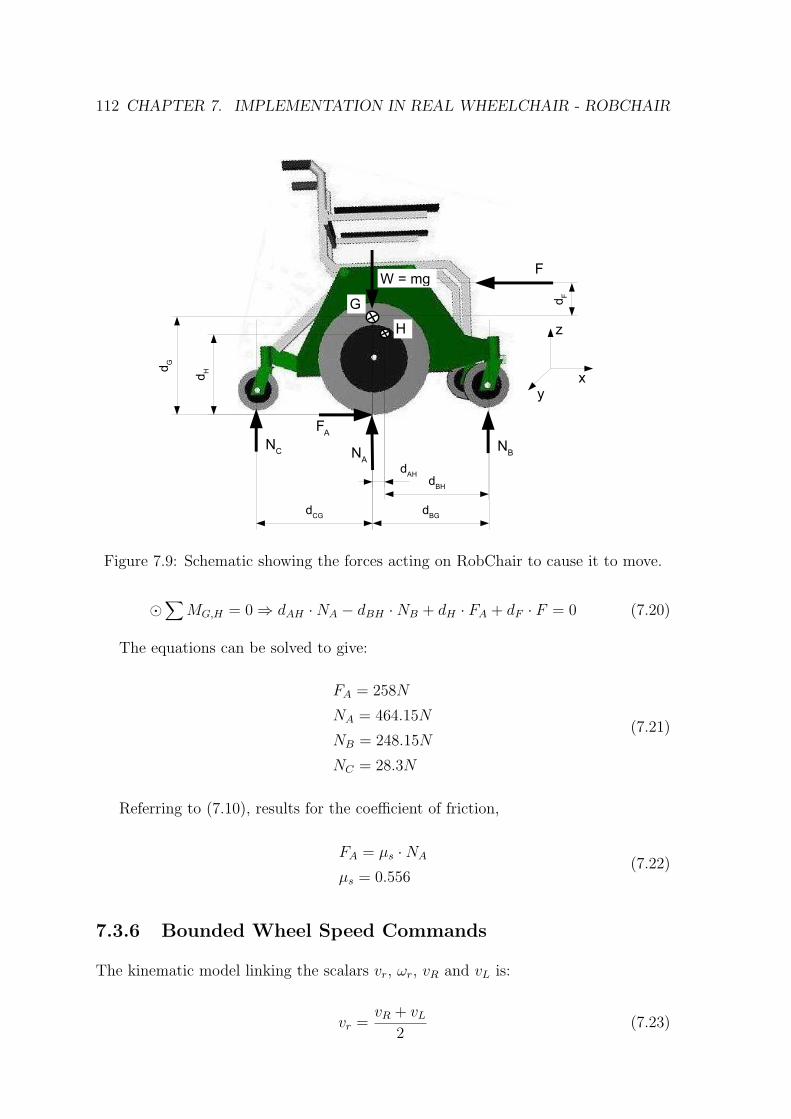
112 CHAPTER 7. IMPLEMENTATION IN REAL WHEELCHAIR - ROBCHAIR
Figure 7.9: Schematic showing the forces acting on RobChair to cause it to move.
⊙∑
MG,H = 0⇒ dAH ·NA − dBH ·NB + dH · FA + dF · F = 0 (7.20)
The equations can be solved to give:
FA = 258N
NA = 464.15N
NB = 248.15N
NC = 28.3N
(7.21)
Referring to (7.10), results for the coefficient of friction,
FA = µs ·NA
µs = 0.556(7.22)
7.3.6 Bounded Wheel Speed Commands
The kinematic model linking the scalars vr, ωr, vR and vL is:
vr =vR + vL
2(7.23)
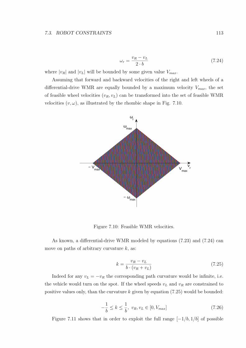
7.3. ROBOT CONSTRAINTS 113
ωr =vR − vL
2 · b(7.24)
where |vR| and |vL| will be bounded by some given value Vmax.
Assuming that forward and backward velocities of the right and left wheels of a
differential-drive WMR are equally bounded by a maximum velocity Vmax, the set
of feasible wheel velocities (vR, vL) can be transformed into the set of feasible WMR
velocities (v, ω), as illustrated by the rhombic shape in Fig. 7.10.
−2.5 −2 −1.5 −1 −0.5 0 0.5 1 1.5 2 2.5−8
−6
−4
−2
0
2
4
6
8
Vmax
− Vmax
vr
ωmax
− ωmax
ωr
Figure 7.10: Feasible WMR velocities.
As known, a differential-drive WMR modeled by equations (7.23) and (7.24) can
move on paths of arbitrary curvature k, as:
k =vR − vL
b · (vR + vL)(7.25)
Indeed for any vL = −vR the corresponding path curvature would be infinite, i.e.
the vehicle would turn on the spot. If the wheel speeds vL and vR are constrained to
positive values only, than the curvature k given by equation (7.25) would be bounded:
−1
b≤ k ≤
1
b, vR, vL ∈ [0, Vmax] (7.26)
Figure 7.11 shows that in order to exploit the full range [−1/b, 1/b] of possible
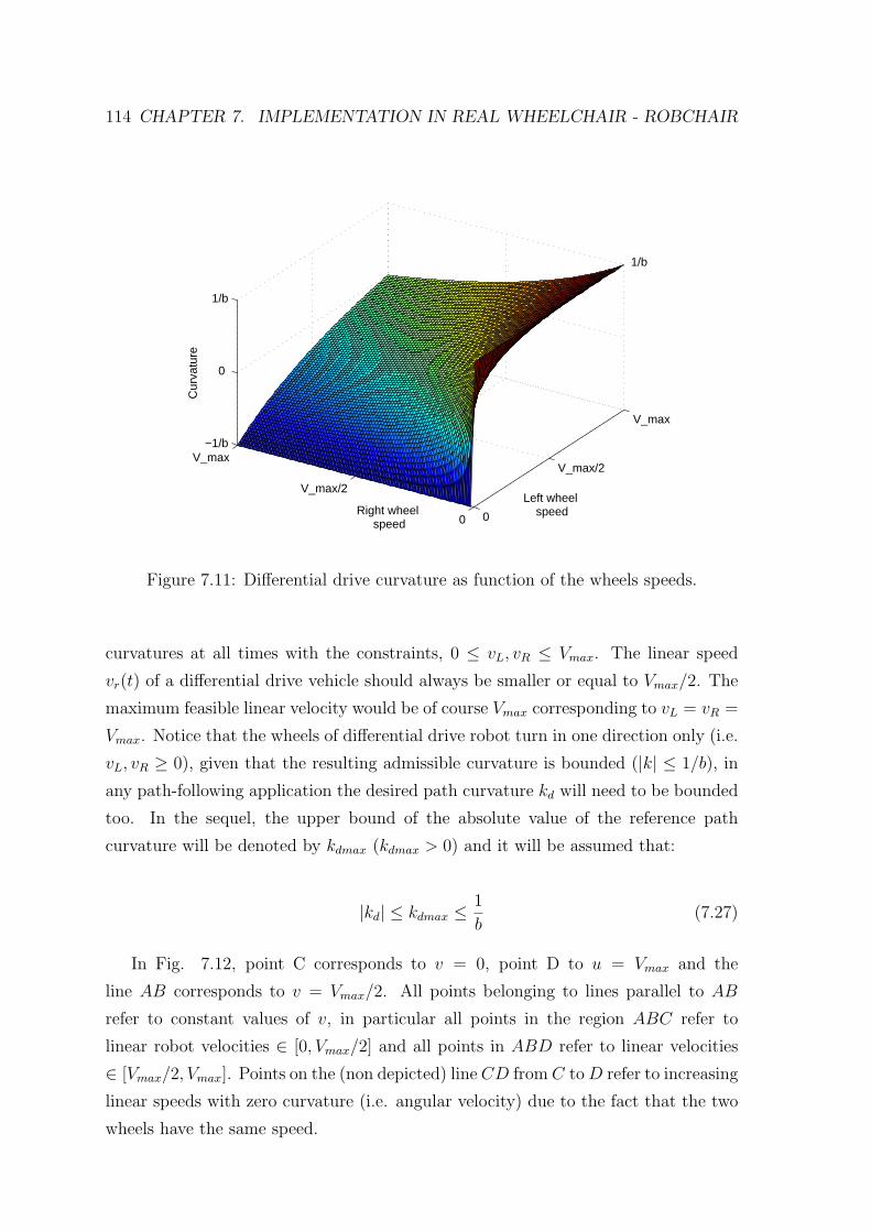
114 CHAPTER 7. IMPLEMENTATION IN REAL WHEELCHAIR - ROBCHAIR
0
V_max/2
V_max
0
V_max/2
V_max−1/b
0
1/b
Left wheel speedRight wheel
speed
Cur
vatu
re
1/b
Figure 7.11: Differential drive curvature as function of the wheels speeds.
curvatures at all times with the constraints, 0 ≤ vL, vR ≤ Vmax. The linear speed
vr(t) of a differential drive vehicle should always be smaller or equal to Vmax/2. The
maximum feasible linear velocity would be of course Vmax corresponding to vL = vR =
Vmax. Notice that the wheels of differential drive robot turn in one direction only (i.e.
vL, vR ≥ 0), given that the resulting admissible curvature is bounded (|k| ≤ 1/b), in
any path-following application the desired path curvature kd will need to be bounded
too. In the sequel, the upper bound of the absolute value of the reference path
curvature will be denoted by kdmax (kdmax > 0) and it will be assumed that:
|kd| ≤ kdmax ≤1
b(7.27)
In Fig. 7.12, point C corresponds to v = 0, point D to u = Vmax and the
line AB corresponds to v = Vmax/2. All points belonging to lines parallel to AB
refer to constant values of v, in particular all points in the region ABC refer to
linear robot velocities ∈ [0, Vmax/2] and all points in ABD refer to linear velocities
∈ [Vmax/2, Vmax]. Points on the (non depicted) line CD from C toD refer to increasing
linear speeds with zero curvature (i.e. angular velocity) due to the fact that the two
wheels have the same speed.
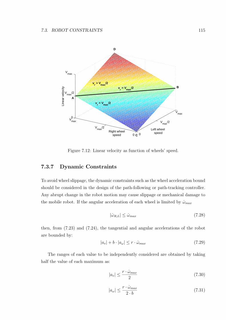
7.3. ROBOT CONSTRAINTS 115
00
0
Left wheel speedRight wheel
speed
Line
ar v
eloc
ity
Vmax
Vmax
Vmax V
max/2
Vmax
/2
Vmax
/2
D
B
A
C
vr = V
max/2
vr > V
max/2
vr < V
max/2
Figure 7.12: Linear velocity as function of wheels’ speed.
7.3.7 Dynamic Constraints
To avoid wheel slippage, the dynamic constraints such as the wheel acceleration bound
should be considered in the design of the path-following or path-tracking controller.
Any abrupt change in the robot motion may cause slippage or mechanical damage to
the mobile robot. If the angular acceleration of each wheel is limited by ωmax
|ωR,L| ≤ ωmax (7.28)
then, from (7.23) and (7.24), the tangential and angular accelerations of the robot
are bounded by:
|av|+ b · |aω| ≤ r · ωmax (7.29)
The ranges of each value to be independently considered are obtained by taking
half the value of each maximum as:
|av| ≤r · ωmax
2(7.30)
|aω| ≤r · ωmax
2 · b(7.31)
116 CHAPTER 7. IMPLEMENTATION IN REAL WHEELCHAIR - ROBCHAIR
7.3.8 Feasible Constraints
Using the constraints in the previous section, the values for the maximum velocity,
acceleration, and deceleration can be obtained as follows:
vd(t) ≤ Vlim
ad(t) ≤ Alim
dd(t) ≥ Dlim
(7.32)
whereVlim = min (vr, vslide)
Alim = min (ar, aslip, aw)
Dlim = min (dr, dslip)
(7.33)
where vr, vslide, ar, aslip, dr, dslip, are obtained from equations (7.1), (7.9), (7.2),
(7.15), (7.3), (7.16) respectively.
7.4 Experimental Results
A set of experimental tests, using RobChair [136], [137], has been performed to eval-
uate the performance of the sliding mode controllers (SM-TT and SM-PF), and the
trajectory planning algorithm with comfort constraint.
According to the notation shown in Fig. 7.4, the RobChair parameter values are
L = 0.614m and R = 0.175m. For all the experiments, the following values of the
SM-TT and SM-PF controllers (see (5.60), (5.61) for SM-TT and (5.60), (5.78), (5.79)
for SM-PF )were used: k0 = 4, k1 = 0.75, k2 = 5, p1 = 0.05, p2 = 0.05, q1 = 0.75,
q2 = 1.75. The signum functions in the command signals were replaced by saturation
functions with ±0.15 thresholds, to reduce the chattering phenomenon.
7.4.1 Experimental Results Under Odometry Navigation
As shown in Fig. 7.13, the first experiment reported here concerns the implementation
of the SM-TT in the following conditions: 1) only odometry feedback is used; 2) initial
pose error (xe = −1, ye = −1 and φe = 0). The same figure shows that the RobChair
retrieved quickly (∆t ≈ 10s) and smoothly from its initial state error, and the tracking
errors converge on average to zero with acceptable reduced values along the path.
Experimental results for SM-TT controller under odometry navigation (without
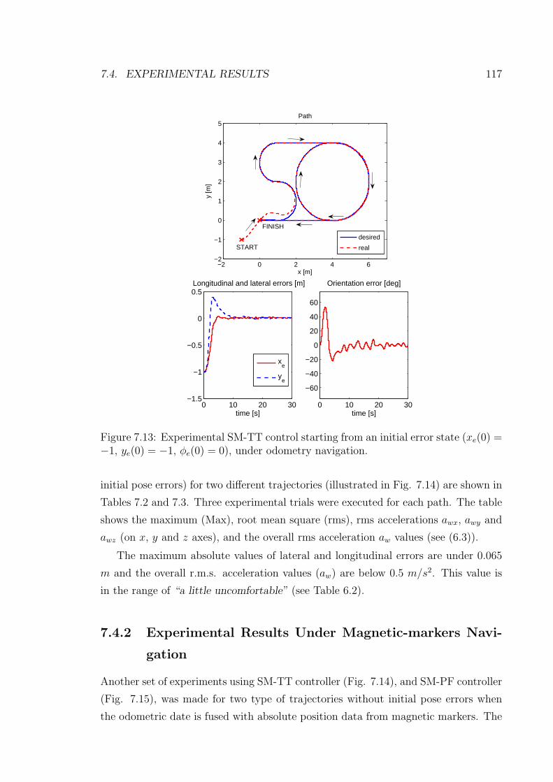
7.4. EXPERIMENTAL RESULTS 117
−2 0 2 4 6−2
−1
0
1
2
3
4
5Path
x [m]
y [m
]
desired
realSTART
FINISH
0 10 20 30−1.5
−1
−0.5
0
0.5 Longitudinal and lateral errors [m]
time [s]
xe
ye
0 10 20 30
−60
−40
−20
0
20
40
60
Orientation error [deg]
time [s]
Figure 7.13: Experimental SM-TT control starting from an initial error state (xe(0) =−1, ye(0) = −1, φe(0) = 0), under odometry navigation.
initial pose errors) for two different trajectories (illustrated in Fig. 7.14) are shown in
Tables 7.2 and 7.3. Three experimental trials were executed for each path. The table
shows the maximum (Max), root mean square (rms), rms accelerations awx, awy and
awz (on x, y and z axes), and the overall rms acceleration aw values (see (6.3)).
The maximum absolute values of lateral and longitudinal errors are under 0.065
m and the overall r.m.s. acceleration values (aw) are below 0.5 m/s2. This value is
in the range of “a little uncomfortable” (see Table 6.2).
7.4.2 Experimental Results Under Magnetic-markers Navi-
gation
Another set of experiments using SM-TT controller (Fig. 7.14), and SM-PF controller
(Fig. 7.15), was made for two type of trajectories without initial pose errors when
the odometric date is fused with absolute position data from magnetic markers. The
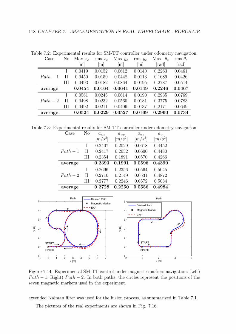
118 CHAPTER 7. IMPLEMENTATION IN REAL WHEELCHAIR - ROBCHAIR
Table 7.2: Experimental results for SM-TT controller under odometry navigation.Case No Max xe rms xe Max ye rms ye Max. θe rms θe
[m] [m] [m] [m] [rad] [rad]
I 0.0419 0.0152 0.0612 0.0140 0.2263 0.0461Path− 1 II 0.0450 0.0159 0.0448 0.0113 0.1689 0.0426
III 0.0493 0.0182 0.0864 0.0195 0.2787 0.0514average 0.0454 0.0164 0.0641 0.0149 0.2246 0.0467
I 0.0581 0.0245 0.0614 0.0190 0.2935 0.0769Path− 2 II 0.0498 0.0232 0.0560 0.0181 0.3775 0.0783
III 0.0492 0.0211 0.0406 0.0137 0.2171 0.0649average 0.0524 0.0229 0.0527 0.0169 0.2960 0.0734
Table 7.3: Experimental results for SM-TT controller under odometry navigation.Case No awx awy awz aw
[m/s2] [m/s2] [m/s2] [m/s2]
I 0.2407 0.2029 0.0618 0.4452Path− 1 II 0.2417 0.2052 0.0600 0.4480
III 0.2354 0.1891 0.0570 0.4266average 0.2393 0.1991 0.0596 0.4399
I 0.2696 0.2356 0.0564 0.5045Path− 2 II 0.2710 0.2149 0.0531 0.4872
III 0.2777 0.2246 0.0572 0.5034average 0.2728 0.2250 0.0556 0.4984
−1 0 1 2 3 4 5 6 7−1
0
1
2
3
4
5
x [m]
y [m
]
Path
Desired Path
Magnetic Marker
EKF
FINISH
START
−2 0 2 4 6−1
0
1
2
3
4
5
x [m]
y [m
]
Path
Desired Path
Magnetic Marker
EKF
START
FINISH
Figure 7.14: Experimental SM-TT control under magnetic-markers navigation: Left)Path − 1; Right) Path− 2. In both paths, the circles represent the positions of theseven magnetic markers used in the experiment.
extended Kalman filter was used for the fusion process, as summarized in Table 7.1.
The pictures of the real experiments are shown in Fig. 7.16.
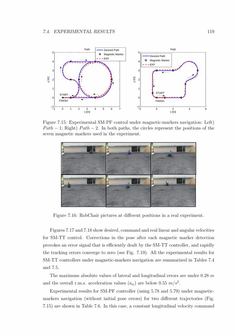
7.4. EXPERIMENTAL RESULTS 119
−1 0 1 2 3 4 5 6 7−1
0
1
2
3
4
5
x [m]
y [m
]Path
Desired Path
Magnetic Marker
EKF
START
FINISH
−2 0 2 4 6−1
0
1
2
3
4
5
x [m]
y [m
]
Path
Desired Path
Magnetic Marker
EKF
START
FINISH
Figure 7.15: Experimental SM-PF control under magnetic-markers navigation: Left)Path − 1; Right) Path− 2. In both paths, the circles represent the positions of theseven magnetic markers used in the experiment.
Figure 7.16: RobChair pictures at different positions in a real experiment.
Figures 7.17 and 7.18 show desired, command and real linear and angular velocities
for SM-TT control. Corrections in the pose after each magnetic marker detection
provokes an error signal that is efficiently dealt by the SM-TT controller, and rapidly
the tracking errors converge to zero (see Fig. 7.19). All the experimental results for
SM-TT controllers under magnetic-markers navigation are summarized in Tables 7.4
and 7.5.
The maximum absolute values of lateral and longitudinal errors are under 0.28 m
and the overall r.m.s. acceleration values (aw) are below 0.55 m/s2.
Experimental results for SM-PF controller (using 5.78 and 5.79) under magnetic-
markers navigation (without initial pose errors) for two different trajectories (Fig.
7.15) are shown in Table 7.6. In this case, a constant longitudinal velocity command
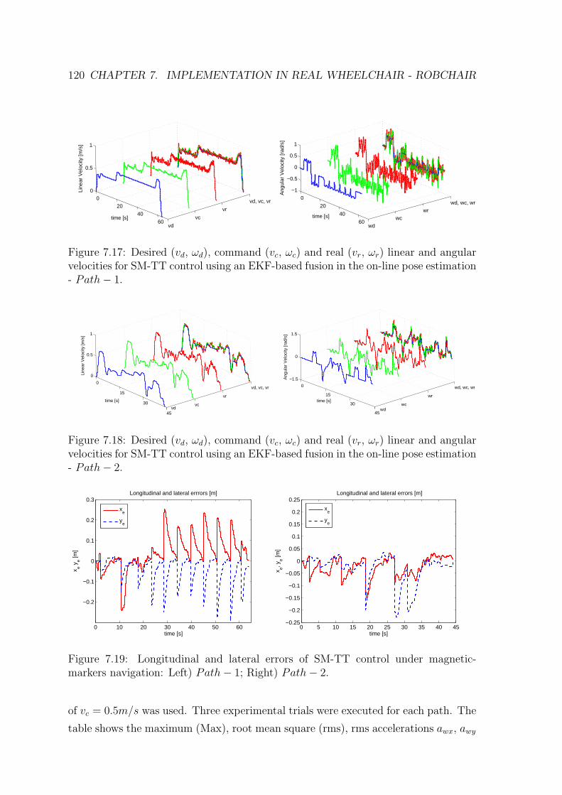
120 CHAPTER 7. IMPLEMENTATION IN REAL WHEELCHAIR - ROBCHAIR
vd, vc, vr
vr
vc
vd
0
20
40
60
0
0.5
1
time [s]
Line
ar V
eloc
ity [m
/s]
wd, wc, wr
wr
wc
wd
0
20
40
60
−1
−0.5
0
0.5
1
time [s]
Ang
ular
Vel
ocity
[rad
/s]
Figure 7.17: Desired (vd, ωd), command (vc, ωc) and real (vr, ωr) linear and angularvelocities for SM-TT control using an EKF-based fusion in the on-line pose estimation- Path− 1.
vd, vc, vr
vr
vc
0
15
30
45
0
0.5
1
time [s]
Line
ar V
eloc
ity [m
/s]
vd
wd, wc, wr
wr
wc
0
15
30
45
−1.5
0
1.5
time [s]
Ang
ular
Vel
ocity
[rad
/s]
wd
Figure 7.18: Desired (vd, ωd), command (vc, ωc) and real (vr, ωr) linear and angularvelocities for SM-TT control using an EKF-based fusion in the on-line pose estimation- Path− 2.
0 10 20 30 40 50 60
−0.2
−0.1
0
0.1
0.2
0.3
time [s]
x e ye [m
]
Longitudinal and lateral errrors [m]
xe
ye
0 5 10 15 20 25 30 35 40 45−0.25
−0.2
−0.15
−0.1
−0.05
0
0.05
0.1
0.15
0.2
0.25 Longitudinal and lateral errors [m]
time [s]
x e, ye [m
]
xe
ye
Figure 7.19: Longitudinal and lateral errors of SM-TT control under magnetic-markers navigation: Left) Path− 1; Right) Path− 2.
of vc = 0.5m/s was used. Three experimental trials were executed for each path. The
table shows the maximum (Max), root mean square (rms), rms accelerations awx, awy
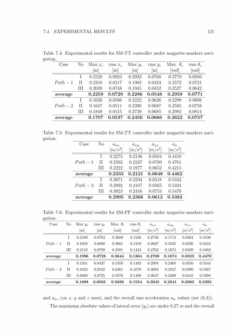
7.4. EXPERIMENTAL RESULTS 121
Table 7.4: Experimental results for SM-TT controller under magnetic-markers navi-gation.
Case No Max xe rms xe Max ye rms ye Max. θe rms θe
[m] [m] [m] [m] [rad] [rad]
I 0.2528 0.0923 0.2932 0.0768 0.3779 0.0950Path− 1 II 0.2210 0.0517 0.1982 0.0424 0.2572 0.0721
III 0.2039 0.0748 0.1945 0.0452 0.2527 0.0642average 0.2259 0.0729 0.2286 0.0548 0.2959 0.0771
I 0.1626 0.0586 0.2222 0.0626 0.2299 0.0698Path− 2 II 0.1647 0.0511 0.2390 0.0687 0.2585 0.0758
III 0.1849 0.0515 0.2739 0.0685 0.2982 0.0814average 0.1707 0.0537 0.2450 0.0666 0.2622 0.0757
Table 7.5: Experimental results for SM-TT controller under magnetic-markers navi-gation.
Case No awx awy awz aw
[m/s2] [m/s2] [m/s2] [m/s2]
I 0.2275 0.2138 0.0584 0.4410Path− 1 II 0.2502 0.2247 0.0709 0.4761
III 0.2222 0.1977 0.0652 0.4215average 0.2333 0.2121 0.0648 0.4462
I 0.3071 0.2234 0.0518 0.5342Path− 2 II 0.2892 0.2447 0.0565 0.5334
III 0.3023 0.2416 0.0753 0.5470average 0.2995 0.2366 0.0612 0.5382
Table 7.6: Experimental results for SM-PF controller under magnetic-markers navi-gation.
Case No Max ye rms ye Max. θe rms θe awx awy awz aw
[m] [m] [rad] [rad] [m/s2] [m/s2] [m/s2] [m/s2]
I 0.2189 0.0704 0.3689 0.1348 0.2736 0.1713 0.0304 0.4530
Path− 1 II 0.1658 0.0690 0.3661 0.1319 0.2687 0.1635 0.0326 0.4416
III 0.2142 0.0789 0.3581 0.1424 0.2702 0.1674 0.0339 0.4463
average 0.1996 0.0728 0.3644 0.1364 0.2708 0.1674 0.0323 0.4470
I 0.1341 0.0437 0.5350 0.1493 0.2994 0.2468 0.0350 0.5444
Path− 2 II 0.1642 0.0532 0.6261 0.1679 0.3094 0.2247 0.0390 0.5367
III 0.2680 0.0725 0.5878 0.1489 0.3047 0.2309 0.0410 0.5368
average 0.1888 0.0565 0.5830 0.1554 0.3045 0.2341 0.0383 0.5393
and awz (on x, y and z axes), and the overall rms acceleration aw values (see (6.3)).
The maximum absolute values of lateral error (ye) are under 0.27m and the overall
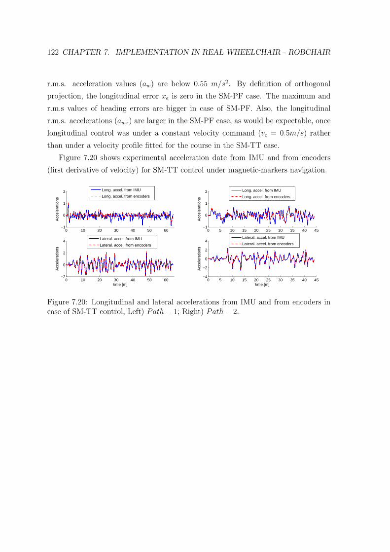
122 CHAPTER 7. IMPLEMENTATION IN REAL WHEELCHAIR - ROBCHAIR
r.m.s. acceleration values (aw) are below 0.55 m/s2. By definition of orthogonal
projection, the longitudinal error xe is zero in the SM-PF case. The maximum and
r.m.s values of heading errors are bigger in case of SM-PF. Also, the longitudinal
r.m.s. accelerations (awx) are larger in the SM-PF case, as would be expectable, once
longitudinal control was under a constant velocity command (vc = 0.5m/s) rather
than under a velocity profile fitted for the course in the SM-TT case.
Figure 7.20 shows experimental acceleration date from IMU and from encoders
(first derivative of velocity) for SM-TT control under magnetic-markers navigation.
0 10 20 30 40 50 60−1
0
1
2
Acc
eler
atio
ns
Long. accel. from IMU
Long. accel. from encoders
0 10 20 30 40 50 60−2
0
2
4
time [m]
Acc
eler
atio
ns
Lateral. accel. from IMU
Lateral. accel. from encoders
0 5 10 15 20 25 30 35 40 45−1
0
1
2
Acc
eler
atio
ns
Long. accel. from IMU
Long. accel. from encoders
0 5 10 15 20 25 30 35 40 45−4
−2
0
2
4
time [m]
Acc
eler
atio
ns
Lateral. accel. from IMU
Lateral. accel. from encoders
Figure 7.20: Longitudinal and lateral accelerations from IMU and from encoders incase of SM-TT control, Left) Path− 1; Right) Path− 2.
Chapter 8
Conclusions
This thesis describes trajectory-tracking and path-following controllers based on the
sliding-mode theory for WMRs and autonomous vehicles. Moreover, a trajectory
planning algorithm is described that deals with comfort constraints providing smooth
trajectories with low associated accelerations. The proposed control structure is based
on two nonlinear sliding surfaces ensuring the tracking of the three output variables,
exploiting the nonholonomic constraint. The control law has been thoroughly eval-
uated in terms of tracking performance either by simulation and real experiments.
Using the trajectory planner, trajectories are generated that comply with user com-
fort requirements by exposing him/her to acceptable levels of accelerations, being its
maximum value a design parameter.
The experimental tests presented in this thesis are representative of the average
performance of the controllers. I had summarized my acquired experience in general
observations that can be useful guidelines for implementation of the same control
strategies in other type of mobile robots.
The following suggestions are recommended for future work:
• It would be interesting to study the sliding-mode control design using the WMR
dynamical model, where uncertainties in the robot physical parameters exist.
• The performances of the four reaching laws (Chapter 5) can by compared in
order to establish an on-line parameters adjusting procedure and deserves more
study.
• The trajectory planners that work directly with a library of skills (percep-
tion and motor skills) should be investigated, instead of working with prepro-
grammed planners.
123
124 CHAPTER 8. CONCLUSIONS
The topic of nonlinear control systems is large and receives a lot of research inter-
est in both journals and conferences. This thesis has touched aspects with relevance
to controller design, robotics and in particular mobile robotics. Questions have been
answered, new ones have appeared. With the appearance of smarter sensors, faster
computers, and more reliable data processing, the design and implementation of non-
linear control techniques for mobile robotics are of great interest and should attract
further investigations.
Appendix A
Appendix
Definition (G1-curves): A parametric curve p(u) has first-order geometric conti-
nuity, and we say p(u) is a G1-curve, if p(u) is regular and its unit tangent vector is
a continuous function along the curve, i.e., τ(·) ∈ C0 ([u0, u1]).
Definition (G2-curves): A parametric curve p(u) has second-order geometric
continuity, and we say p(u) is a G2-curve, if p(u) is G1-curve and its curvature vector
is continuous along the curve.
Definition (Comfort): from http://www.websters-online-dictionary.org/
1. a state of being relaxed and feeling no pain;
2. a feeling of freedom from worry or disappointment;
3. the act of consoling; giving relief in affliction.
Barbalat’s Lemma : from Khalil Lemma 8.2 [138], let φ : ℜ → ℜ be a uniformly
continuous function on [0,∞). Suppose that
limt→∞
∫ t
0φ(τ)dτ (A.1)
exists and is finite. Then, φ(t)→ 0 as t→∞.
Extension of Barbalat’s Lemma : Barbalat’s lemma is extended to show
global asymptotic stability in Khalil Theorem 8.4 [138]. Let D ⊂ ℜn be a domain
containing x = 0 and suppose f(t, x) is piecewise continuous in t and locally Lipschitz
in x. Let V be a continuously differentiable function such that
W1(x) ≤ V (x) ≤ W2(x)V (x) ≤ −W (x) (A.2)
125
126 APPENDIX A. APPENDIX
for all x ∈ D, where W1(x) and W2(x) are continuous positive definite functions
and W (x) is a continuous positive semidefinite function on D. Choose r > 0 such
that Br ⊂ D and let ρ < min‖x‖=rW1(x). Then all solutions of x = f(x) with
x(0) ∈ x ∈ Br|W2(x) ≤ ρ are bounded and satisfy
W (x)→ 0 as t→∞ (A.3)
If all of the above assumptions hold globally and W1(x) is radially unbounded, the
statement is true for all x(0) ∈ ℜn.
Global Asymptotic Lyapunov Stability From Khalil Theorem 4.2 [138], let
a general nonlinear, time invariant system x = f(x), have an equilibrium point at
x = 0. System equilibrium points not located at x = 0 may be moved to the origin
through a suitable coordinate transformation. Define a continuously differentiable
Lyapunov function V : ℜn → ℜ such that
V (0) = 0 and V (x) > 0, ∀x 6= 0 ‖x‖ → ∞⇒ V (x)→∞V (x) < 0, ∀x 6= 0 (A.4)
then the origin x = 0 is globally asymptotically stable. This implies the system has
only one equilibrium point.
LaSalle’s Theorem From Khalil Theorem 4.4 [138], let Ω ⊂ D be a compact
set that is positively invariant with respect to x = f(x). Let V : ℜn → ℜ be a
continuously differentiable function such that V (x) ≤ 0 in Ω. Let E be the set of all
points in Ω where V (x) = 0. Let M be the largest invariant set in E. Then every
solution starting in Ω approaches M as t→∞.
This may be extended to asymptotic stability by Khalil Corollary 4.2 [138], let
x = 0 be an equilibrium point for x = f(x). Let V : ℜn → ℜ be a continuously
differentiable, radially unbounded, positive definite function such that V (x) ≤ 0 for
all x ∈ ℜn. Let S =
x ∈ ℜn|V (x) = 0
and suppose that no solution can stay
identically in S, other than the trivial solution x(t) ≡ 0. Then, the origin is globally
asymptotically stable.
The benefit of LaSalle’s theorem is that it does not require V to be negative
definite for global asymptotic stability.
Bibliography
[1] Masehian E. and Katebi Y. (2007). Robot Motion Planning in Dynamic Envi-
ronments with Moving Obstacles and Target, International Journal of Mechan-
ical Systems Science and Engineering, 1(1), 20–25.
[2] Shiller Z., Large F., Sekhavat S. and Laugier C. (2007). Motion Planning in
Dynamic Environments, Autonomous Navigation in Dynamic Environments,
Vol. 35, Springer-Verlag, 107–119.
[3] Wang M. and Liu J.N.K. (2008). Fuzzy Logic-based Real-time Robot Navigation
in Unknown Environment with Dead Ends, Robotics and Autonomous Systems,
Elsevier, 56(7), 625–643.
[4] Fatmi A., Yahmadi A., Khriji L. and Masmoudi N. (2005). A Fuzzy Logic Based
Navigation of a Mobile Robot, International Journal of Applied Mathematics
and Computer Sciences, 1(2), 87–92.
[5] Zavlangas P.G., Tzafestas S.G. and Althoefer K. (2000). Fuzzy Obstacle Avoid-
ance and Navigation for Omnidirectional Mobile Robots, European Symposium
on Intelligent Techniques - ESIT 2000, 375–382.
[6] Lebedev D.V., Steil J.J. and Ritter H.J. (2005). The Dynamic Wave Expansion
Neural Network Model for Robot Motion Planning in Time-varying Environ-
ments, Neural Networks, Elsevier, 18(3), 267–285.
[7] Yang S.X., Hu T., Yuan X., Liu, P.X., Meng M. (2003). A Neural Network
Based Torque Controller for Collision-free Navigation of Mobile Robots, IEEE
International Conference on Robotics and Automation, 1, 13–18.
[8] Kulic R., Vukic Z. (2003). Methodology of Concept Control Synthesis to Avoid
Unmoving and Moving Obstacles, Journal of Intelligent and Robotic Systems,
Springer-Verlag, 37(1), 21–41.
127
128 BIBLIOGRAPHY
[9] Kulic R., Vukic Z. (2006). Methodology of Concept Control Synthesis to Avoid
Unmoving and Moving Obstacles II, Journal of Intelligent and Robotic Systems,
Springer-Verlag, 45(3), 267–294.
[10] Ye C. and Wang D. (2001). A Novel Navigation Method for Autonomous Mobile
Vehicles, Journal of Intelligent and Robotic Systems, Springer-Verlag, 32(4),
361–388.
[11] Zhuang Hui-Zhong, Du Shu-Xin anf Wu Tie-Jun (2006). On-line Real-time
Path Planning of Mobile Robots in Dynamic Uncertain Environment, Journal
of Zhejiang University - Science A, Zhejiang University Press, co-published with
Springer-Verlag, 7(4), 516–524.
[12] Shi Chao-Xia, Hong Bing-Rong, Wang Yan-Qing and Piao Song-Hao. (2006).
Autonomous Navigation Based on the Velocity Space Method in Dynamic En-
vironments, Lecture Notes in Computer Science, Springer-Verlag, 4222/2006,
958–961.
[13] Bloch A. M., McClamroch N. H. and Reyhanoglu M. (1990). Controllability and
Stabilizability of Properties of a Nonholonomic Control Systems, Proc. IEEE
Conf. Decision and Control, 1312-1314.
[14] Divelbiss A. W. and Wen J. T. (1997). Trajectory Tracking Control of a Car-
trailer System, IEEE Transactions Control Systems Technology, 5(3), 269-278.
[15] Bloch, A. M. and McClamroch, N. H. (1989). Control of Mechanical Systems
With Classical non Holonomic Constraints, Proceeding of the 28th IEEE Conf.
on Decision and Control, Tampa, 201–205.
[16] Samson C. and Ait-Abderrahim K. (1991). Feedback Control of a Nonholo-
nomic Wheeled Cart in Cartesian Space, Proceedings of IEEE International
Conference on Robotics and Automation, 2, 1136-1141.
[17] Pomet J. B. (1992). Explicit Design of Time-varying Stabilizing Control Laws
for a Class of Controllable Systems Without Drift, Systems and Control Lett.,
18, 147-158.
[18] MCloskey R. T. and Murray R. M. (1994), Exponential Stabilization of Driftless
Nonlinear Control Systems Using Homogeneous Feedback, IEEE Transactions
on Automatic Control, 42(5), 614–628.
BIBLIOGRAPHY 129
[19] Kanayama Y., Kimura Y., Miyazaki F. and Noguchi T. (1990). A Stable Track-
ing Control Method for an Autonomous Mobile Robot, Proceedings of IEEE
International Conference on Robotics and Automation, 1, 384-389.
[20] Jiang Z.-P. and Nijmeijer H. (1997). Tracking Control of Mobile Robots: A
Case Study in Backstepping, Automatica, 33(7), 1393–1399.
[21] De Luca A. and Oriolo G. (1995). Modelling and Control of Nonholonomic
Mechanical Systems, in: J. Angeles, A. Kecskemethy (Editors), Kinematics
and Dynamics of Multi-Body Systems, Springer-Verlag, 277–342.
[22] Oriolo G., De Luca A. and Vendittelli M. (2002). WMR Control Via Dynamic
Feedback Linearization: Design, Implementation, and Experimental Validation.
IEEE Transactions on Control System Technology, 10(6), 835–852.
[23] Sarkar, N., Yun, X. and Kumar, V. (1992). Control of Mechanical Systems
With Rolling Constraints: Application to Dynamic Control of Mobile Robots
- Technical Report, University of Pennsylvania Department of Computer and
Information Science, Technical Report No. MS-CIS-92-44.
[24] Samson, C. (1993). Time-varying Feedback Stabilization of Car-like Wheeled
Mobile Robots. Int. Journal of Robotics Research, 12(1), 55-64.
[25] Zhang M. and Hirschorn R. M. (1997). Discontinuous Feedback Stabilization of
Nonholonomic Wheeled Mobile Robots, Dynamics and Control, 7(2), 155–169.
[26] Koh K.C. and Cho H.S. (1999). A Smooth Path Tracking Algorithm for Wheeled
Mobile Robots with Dynamic Constraints, Journal of Intelligent and Robotic
Systems, 24(4), 367–385.
[27] Zhang Y., Chung J. H. and Velinsky S.A. (2003). Variable Structure Control
of a Differentially Steered Wheeled Mobile Robot, Journal of Intelligent and
Robotic Systems, 36(3), 301–314.
[28] Yang, J.M. and Kim, J.H. (1999). Sliding Mode Control for Trajectory Tracking
of Nonholonomic Wheeled Mobile Robots, IEEE Transactions on Robotics and
Automation, 15(3), 578-587.
[29] Kim M.S., Shin J.H. and Lee J.J. (2000). Design of a Robust Adaptive Con-
troller for a Mobile Robot, Proc. IEEE/RSJ Int. Conf. On Intelligent Robots
and Systems, 3, 1816-1826.
130 BIBLIOGRAPHY
[30] Fukao T., Nakagawa H., and Adachi N. (2000). Adaptive Tracking Control of a
Nonholonomic Mobile Robot, IEEE Transactions on Robotics and Automation,
16(5), 609-615.
[31] Coelho P. and Nunes U. (2005). Path-following Control of Mobile Robots in
Presence of Uncertainties, IEEE Transactions on Robotics , 21(2), 252-261.
[32] Li C.K. and Chao H.M. (2002). Output Tracking of Uncertain Robot Systems
Via High Order Sliding Mode Technique, Electronic letters, 38(10), 487-489.
[33] Corradini M.L. and Orlando G. (2002). Control of Mobile Robots with Uncer-
tainties in the Dynamical Model: a Discrete Time Sliding Mode Approach with
Experimental Results, Control Engineering Practice, 10(1), 23–34.
[34] Wu S.-F., Mei J.-S. and Niu P.-Y. (2001). Path Guidance and Control of a
Guided Wheeled Mobile Robot, Control Engineering Practice, 9(1), 97–105.
[35] Jiang Z.-P., Lefeber E. and Nijmeijer H. (2001). Saturated Stabilization and
Tracking of a Nonholonomic Mobile Robot, Systems and Control Letters, 42(5),
327–332.
[36] Pourboghrat F. and Karlsson M. P. (2002). Adaptive Control of Dynamic Mo-
bile Robots with Nonholonomic Constraints, Computers and Electrical Engi-
neering, 28(4), 241–253.
[37] Dong W. and Kuhnert K.-D. (2005). Robust Adaptive Control of Nonholo-
nomic Mobile Robot with Parameter and Nonparameter Uncertainties, IEEE
Transactions on Robotics, 21(2), 261-266.
[38] Fierro R. and Lewis F. L.(1997). Control of a Nonholonomic Mobile Robot:
Backstepping Kinematics into Dynamics. Journal of Robotic Systems, 14(3),
149-163.
[39] Kolmanovsky I. and McClamroch N. H. (1995). Development in Nonholonomic
Control Problems, IEEE Control Systems, 20-36.
[40] Kim Min-Soeng, Shin Jin-Ho, Hong Sun-Gi, and Lee Ju-Jang. (2002). Designing
a Robust Adaptive Dynamic Controller for Nonholonomic Mobile Robots under
Modeling Uncertainty and Disturbances, Mechatronics, 13(5), 507-519.
BIBLIOGRAPHY 131
[41] Dong, W., Huo, W., Tso, S. K. and Xu, W. L. (2000). Tracking Control of Un-
certain Dynamic Nonholonomic System and its Application to Wheeled Mobile
Robots, IEEE Transactions on Robotics and Automation, 16(6), 870-874.
[42] Campion, G., dAndrea-Novel, B. and Bastin, G. (1991). ModeLling and State
Feedback Control of Nonholonomic Mechanical Systems, Proceedings of the 30th
IEEE Conf. on Decision and Control, 1184–1189.
[43] Brockett R.W. (1983). Asymptotic Stability and Feedback Stabilization, Dif-
ferential Geometric Control Theory, Birkhauser, Boston, 181–191.
[44] Canudas de Wit C., Khennouf H., Samson C. and Sordalen O. (1993). Nonlinear
Control Design for Mobile Robots. Recent Trends in Mobile Robotics, Vol. 11,
World Scientific Series in Robotics and Automated Systems, 121-156.
[45] Godhavn J. and Egeland O. (1997). A Lyapunov Approach to Exponential
Stabilization of Nonholonomic Systems in Power Form, IEEE Transactions on
Automatic Control, 42(7), 1028-1032.
[46] Aguiar A., Atassi A. and Pascoal A. (2000). Regulation of a Nonholonomic
Dynamic Wheeled Mobile Robot with Parametric Modeling Uncertainty Us-
ing Lyapunov Function, Proc. 39th IEEE Conference on Decision and Control,
Sidney, Australia, 2995–3000.
[47] Canudas de Wit C. and Sordalen O. (1992). Exponential Stabilization of Mo-
bile Robots with Nonholonomic Constraints, IEEE Transactions on Automatic
Control, 37(11), 17911797.
[48] Hespanha J., Morse A. S. (1999). Stabilization of Nonholonomic Integrators via
Logic-Based Switching. Automatica, Special Issue on Hybrid Systems, 35(3),
385-393.
[49] Freund E. and Mayr R. (1997). Nonlinear Path Control in Automated Vehicle
Guidance, IEEE Transactions on Robotics and Automation, 13(1), 49-60.
[50] Walsh G., Tilbury D., Sastry S., Murray R. and Laumond J.P. (1994). Sta-
bilization of Trajectories for Systems with Nonholonomic Constraints, IEEE
Transactions on Automatic Control, 39(1), 216-222.
132 BIBLIOGRAPHY
[51] Fierro R. and Lewis F. (1995). Control of a Nonholonomic Mobile Robot: Back-
stepping Kinematics into Dynamics, Proc. 34th IEEE Conference on Decision
and Control, New Orleans, LA, USA, 3805-3810.
[52] Micaelli A. and Samson C. (1993). Trajectory Tracking for Unicycle-Type
and Two-Steering-Wheels Mobile Robots, Technical Report No. 2097, INRIA,
France.
[53] Samson C. and Ait-Abderrahim K. (1990). Mobile Robot Control Part 1: Feed-
back Control of A Nonholonomic Wheeled Cart in Cartesian Space, Technical
Report No. 1288, INRIA, France.
[54] Jiang Z. and Nijmeijer H. (1999). A Recursive Technique for Tracking Control
of Nonholonomic Systems in Chained Form, IEEE Transactions on Robotics
and Automation, 44(2), 265279.
[55] Colbaugh R., Barany E., and Glass K. (1998). Adaptive Control of Nonholo-
nomic Robotic Systems, Journal of Robotic Systems, 15(7), pp. 365-393
[56] Tayebi A., Tadjine M., and Rachid A., (2001). Invariant Manifold Approach for
the Stabilization of Nonholonomic Chained Systems: Application to a Mobile
Robot, Nonlinear Dynamics, 24, 167-181.
[57] Fierro R. and Lewis F. L. (1998). Control of a Nonholonomic Mobile Robot
Using Neural Networks, IEEE Transactions on Neural Networks, 9(4), 589-600.
[58] Indiveri G. (1999). Kinematic Time-invariant Control of a 2D Nonholonomic
Vehicle, Proceedings of the 38th Conference on Decision and Control, Phoenix,
USA, 2112-2117.
[59] Astolfi A. (1994). On the Stabilization of Nonholonomic Systems, Proceedings
of the 33rd Conference on Decision and Control, Lake Buena Vista, USA, 3481-
3486.
[60] Aicardi M., Casalino G., Bicchi A. and Balestrino A. (1995). Closed Loop Steer-
ing of Unicycle Like Vehicles Via Lyapunov Techniques, IEEE Robotics and
Automation Magazine, 2, pp. 27-35.
[61] A. Tayebi A. and Rachid A. (1997). A Unified Discontinuous State Feedback
Controller for the Path-following and the Point-stabilization Problems of a
BIBLIOGRAPHY 133
Unicycle-like Mobile Robot, Proceedings of the 1997 IEEE International Con-
ference on Control Applications, Hartford, USA, 31-35.
[62] Altafini C. (2003). Path Following With Reduced Off-Tracking for Multibody
Wheeled Vehicles, IEEE Transaction on Control Systems Technology, 11(4),
598-605.
[63] Samson C. (1995). Control of Chained Systems: Application to Path Following
and Time-varying Point-stabilization of Mobile Robots, IEEE Transaction on
Automatic Control, 40(1), 64-77.
[64] Sampei M., Tamura T., Itoh T. and Nakamichi M. (1991). Path Tracking Con-
trol of Trailer-like Mobile Robot, IEEE/RSJ International Workshop on Intel-
ligent Robots and Systems, IROS91, Osaka, 193-198.
[65] Guldner, J. and Utkin, V. I. (1995). Sliding Mode Control for Gradient Tracking
and Robot Navigation Using Artificial Potential Fields, IEEE Transactions on
Robotics and Automation, 11(2), 247254.
[66] dAndrea Novel, B., Campion, G. and Bastin, G. (1995). Control of Nonholo-
nomic Wheeled Mobile Robots by State Feedback Linearization. Int. J. Robot.
Res., 14(6), 543-559.
[67] Kozlowski, K. and Majchrzak, J. (2002). A Backstepping Approach to Control
a Nonholonomic Mobile Robot. In Proc. IEEE Conf. Robot. Autom., 39723977.
[68] Yang, S.X., Yang, H. and Meng, M. Q.-H. (2004). Neural Dynamics Based Full-
state Tracking Control of a Mobile Robot. In Proc. IEEE Conf. on Robotics
and Automation, 5, 46144619.
[69] De Luca, A., Oriolo, G. and Samson C. (1998). Feedback Control of a Nonholo-
nomic Car-like Robot, Robot Motion Planning and Control, Springer-Verlag,
170-253.
[70] Pacejka, H. B. (2002). Tire and Vehicle Dynamics, Society of Automotive En-
gineers and Butterworth-Heinemann, Oxford.
[71] Malan, S., Milanese, M., Borodani, P. and Gallione, A. (2005). Lateral Control
of Autonomous Vehicle for Public Urban Mobility Systems, Proceedings of IEEE
Conference on Intelligent Transportation Systems, 372-377.
134 BIBLIOGRAPHY
[72] Tondel, P. and Johansen, T. A. (2003). Lateral Vehicle Stabilization Using
Constrained Nonlinear Control, Lateral vehicle stabilization using constrained
nonlinear control, Cambridge.
[73] Meier, G., Roppenecker, G. and Wurmthaler, C. (2004). Automatic Lateral
Vehicle Guidance Using Tracking Control - A Modular Approach to Separate
Driver- and Vehicle-Dependent Dynamics, Proceedings of the IEEE Intelligent
Vehicles Symposium, 145-149.
[74] Choi, S.B. (2000). The design og the Look-Down Feedback Adaptive Controller
for the Lateral Control of Front-Wheel-Steering Autonomous Highway Vehicles,
IEEE Transactions on Vehicular Technology, 49(6), 2257-2269.
[75] Tan, H.S., Guldner J., Patwardhan, S., Chen, C. and Bougler B. (1999). De-
velopment of an Automated Steering Vehicle Based on Roadway Magnets -
A Case Study of Mechatronic System Design, IEEE/ASME Transactions on
Mechatronics, 4(3), 258-272.
[76] Hernandez, J.I. and Kuo, C.Y. (2003). Steering Control of Automated Vehicles
Using Absolute Positioning GPS and Magnetic Markers, IEEE Transactions on
Vehicular Technology, 52(1), 150-161.
[77] Chen, C. and Tan H.S. (1999). Experimental Study of Dynamic Look-Ahead
Scheme for Vehicle Steering Control, Proceeding of the American Control Con-
ference, San Diego, 3163-3167.
[78] Rossetter, E.J. and Gerdes J.C. (2002). A study of Lateral Vehicle Control Un-
der a ’Virtual’ Force Framework. International Symposium on Advanced Vehicle
Control, Japan.
[79] Mammar, S. and Netto, M. (2004). Integrated Longitudinal and Lateral Con-
trol for Vehicle Low Speed Automation, Proceeding of the IEEE International
Conference on Control Applications, 350-355.
[80] Chaibet, A., Nouveliere, L., Mammar, S., Netto, M. and Labayrade, R. (2005).
Backstepping Control Synthesis for Both Longitudinal and Lateral Automated
Vehicle, IEEE Intelligent Vehicles Symposium, 42-47.
[81] Hung, J. Y., Gao, W. and Hung, J. C. (1993). Variable Structure Control: A
Survey. IEEE Transaction on Industrial Electronics, 40(1), 2-22.
BIBLIOGRAPHY 135
[82] Utkin, V. I. (1977). Variable Structure Systems with Sliding Mode. IEEE Trans-
actions on Automatic Control, 22(2), 212-222.
[83] Utkin, V. I. and Young, K. D. (1978). Method for Constructing Discontinu-
ity Planes in Multidimensional Variable Structure Systems. Automation and
Remote Control, 39(10), 1466-1470.
[84] Slotine, J. J. and Sastry, S. S. (1982). Tracking Control of Non-linear Systems
Using Sliding Surfaces, with Application to Robot Manipulators. Massachusetts
Institute of Technology, Cambridge MA 02139, Tehnical Report LIDS-P-1264,
1-54.
[85] Slotine, J. J. and Li, W. (1991). Applied Nonlinear Control. Prentice-Hall, Inc,
Inglewood Cliffs, New Jersey
[86] Utkin, V. I. (1992). Sliding Modes in Control Optimization. New York,
Springer-Verlag.
[87] Young, D. K. and Ozguner, U.(1993). Frequency Shaping Compensator Design
for Sliding Mode. Int. J. Control, 57(5), 1005-1019
[88] DeClarlo, R.A., Zak, S. H. and Mathews, G. R. (1988). Variable Structure
Control of Nonlinear Multivariable Systems: A Tutorial. Proceedings of the
IEEE, 76(3), 212-232.
[89] Gao, W. and Hung, J. C. (1993). Variable Structure Control of Nonlinear Sys-
tems: a New Approach. IEEE Transaction on Industrial Electronics, 40(1),
45-55.
[90] Loh, A.M. and Yeung L.F. (2004). Chattering Reduction in Sliding Mode Con-
trol: An Improvement for Nonlinear Systems, WSEAS Transaction on Systems,
9(3), 2878-2885.
[91] Young, D. K., Utkin,V. I. and Ozguner, U.(1999), A Control Engineer’s Guide
to Sliding Mode Control. IEEE Transaction on Control System Technology,
7(3), 328-342.
[92] Haskara, I. and Ozguner, U. (1999). An Estimation Based Robust Tracking
Controller Design for Uncertain Nonlinear System. Proceedings of the 38th Con-
ference on Decision and Control, Arizona USA, 4816-4821.
136 BIBLIOGRAPHY
[93] Elmali, H. and Olagac, N. (1996). Implementation of Sliding Mode Control
with Perturbation Estimation (SMCPE). IEEE Transaction on Control System
Technology, 4(1), 79-85.
[94] Moura, J. T., Roy, R. G. and Olgac, N. (1997). Sliding Mode Control with
Perturbation Estimation (SMCPE) and Frequency Shaped Sliding Surfaces.
Journal of Dynamic Systems, Measurement, and Control, 119(3), 584-588.
[95] Bartolini, G. and Pydynowski, P. (1996). An Improved, Chattering Free, VSC:
Scheme for Uncertain Dynamical Systems. IEEE Transaction on Automatic
Control, 41(8), 1220-1226.
[96] Bartolini, G., Ferrara, A. and Usai, E. (1998). Chattering Avoidance by Second-
order Sliding Mode Control. IEEE Transactions on Automatic Control, 43(2),
241-246.
[97] Pan, Y. and Furuta, K. (2006). Variable Structure Control with Sliding Sec-
tor for Hybrid Systems. Proceedings of the 2006 International Workshop on
Variable Structure Systems, Alghero, Italy, 286-291.
[98] Jiang, K., Seneviratne, L.D. and Earles, S.W.E (1997). Time-optimal Smooth-
path Motion Planning for a Mobile Robot with Kinematic Constraints. Robotica,
15, 547-553.
[99] Aydin, S. and Temeltas, H. (2004). Fuzzy-Differential Evolution Algorithm for
Planning Time-Optimal Trajectories of a Unicycle Mobile Robot on a Prede-
fined Path. Advanced Robotics, 18(7), 725-748.
[100] Stentz, A. (1993). Optimal and Efficient Path Planning for Unknown and Dy-
namic Environments. Carnegie Mellon University Robotics Institute, Technical
Report CMU-RI-TR-93-20, 1-38.
[101] Louste, C. and Liegeois, A. (2002). Path Planning for Non-holonomic Vehicles:
a Potential Viscous Fluid Field Method. Robotica, 20, 291-298.
[102] Parking, R.E. (1991). Applied Robotic Analysis. Prentice Hall, New Jersey.
[103] Gallina, P. and Gasparetto, A. (2000). A Technique to Analytically Formulate
and to Solve the 2-Dimensional Constrained Trajectory Planning Problem for
a Mobile Robot. Journal of Intelligent and Robotic Systems, 27, 237-262.
BIBLIOGRAPHY 137
[104] Munoz, V., Ollero, A., Prado, M. and Simon, A. (1994). Mobile Robot Tra-
jectory Planning with Dynamic and Kinematic Constraints. Proceedings 1994
IEEE International Conference on Robotics and Automation, 4, 2802-2807.
[105] Lamiraux, F., Sekhavat, S., Laumond, J.P. (1999). Motion Planning and Con-
trol for Hilare Pulling a Trailer. IEEE Transactions on Robotics and Automa-
tion, 15(4), 640-652.
[106] Cherif, M. (1999). Motion Planning for All-Terrain Vehicles: A Physical Mod-
eling Approach for Coping with Dynamic and Contact Interaction Constraints.
IEEE Transactions on Robotics and Automation, 15(2), 202-218.
[107] Fotouhi, R., Szyszkowski, W. and Nikiforuk, P. (2002). Trajectory Planning
and Speed Control for a Two-link Rigid Manipulator. Journal of Mechanical
Design, 124(3), 585-589.
[108] Munoz, V., Cruz, A. and Garcia-Cerezo, A. (1998). Speed Planning and Genera-
tion Approach Based on the Path-time Space for Mobile Robots. Proceedings in
the IEEE International Conference on Robotics and Automation, 3, 2199-2204.
[109] Prado, M., Simon, A. and Ezquerro, F. (2002). Velocity, Acceleration and De-
celeration Bounds for a Time-Optimal Planner of a Wheeled Mobile Robot.
Robotica, 20, 181-193.
[110] Prado, M., Simon, A., Carabias, E., Perez, A. and Ezquerro, F. (2003). Optimal
Velocity Planning of Wheeled Mobile Robots on Specific Paths in Static and
Dynamic Environments. Journal of Robotic Systems, 20(12), 737-754.
[111] Piazzi, A. and Guarino Lo Bianco, C. (2000). Quintic G2-Spline for Trajectory
Planning of Autonomous Vehicles. Proceedings in the IEEE Intelligent Vehicles
Symposium, Dearborn, USA, 198-203.
[112] Guarino Lo Bianco, C. and Piazzi, A. (2000). Optimal Trajectory Planning with
Quintic G2-Spline. Proceedings in the IEEE Intelligent Vehicles Symposium,
Dearborn, USA, 620-625.
[113] Maeda, S., Futatsuka, M., Yonesaki, J. and Ikeda, M. (2003). Relationship
Between Questionnaire Survey Results of Vibration Complaints of Wheelchair
Users and Vibration Transmissibility of Manual Wheelchair. In Health and Pre-
ventive Medicine, 8, 82–89.
138 BIBLIOGRAPHY
[114] Forstberg, J. (2000). Ride Comfort and Motion Sickness in Tilting Trains - Hu-
man Responses to Motion Environments in Train and Simulator Experiments.
Doctoral Thesis, Stockholm.
[115] European-Parliament and the Council of the European Union. (2002). On the
Minimum Health and Safety Requirements Regarding the Exposure of Workers
to the Risks Arising from Physical Agents. Official Journal of the European
Communities, Directive 2002/44/EC.
[116] Atapourfard M., Ishihara T. and Inooka. H. (2002). The Influences of Trunk
Horizontal Vibration to the Head-neck Complex. SICE02, Osaka, 1053–1058.
[117] Atapourfard M., Ishihara T. and Inooka H. (2004). Identification of the Head-
neck Complex in Response to Trunk Horizontal Vibration. Biological Cybernet-
ics, 90(6), 418–426.
[118] Gurses S., Dhaher Y., Hain T.C. and Keshner E.A. (2005). Perturbation Param-
eters Associated with Nonlinear Responses of the Head at Small Amplitudes.
CHAOS, 15(2), 023905.1–023905.10.
[119] Kitazaki S. and Griffin M.J. (1997). A Modal Analysis of Whole-body Vertical
Vibration Using a Finite Element Model of the Human Body. Journal of Sound
and Vibration, 200(1), 83–103.
[120] Van Der Woude, L.H.V., Hopman M.T.E and Kemenade, C.H. (1999) Biomedi-
cal Aspects of Manual Wheelchair Propulsion: The State of the Art II. Assistive
Technology Research Series, 5, 392 pp.
[121] Pires, G. and Nunes, U. (2002). A Wheelchair Steered Through Voice Com-
mands and Assisted by a Reactive Fuzzy-logic Controller, Int. Journal of Intel-
ligent and Robotic Systems, 34(3), 301-314.
[122] Maia, R., Cortesao, R., Nunes, U., Silva, V. and Fonseca, J. (2003). Robust
Low-Level Motion Control of WMR with Stochastic Active Observers, The
11th International Conference on Advanced Robotics, Coimbra, 2, 876-882.
[123] Yanco, H.A. (1998). Wheelesley, a Robotic Wheelchair System: Indoor Navi-
gation and User Interface. In Lecture Notes in Artificial Intelligence: Assistive
Technology and Artificial Intelligence. Springer-Verlag, 256268.
BIBLIOGRAPHY 139
[124] Levine, S.P., Bell, D.A., Jaros, L.A., Simpson, R.C., Koren, Y., and Boren-
stein, J. (1999). The NavChair Assistive Wheelchair Navigation System, IEEE
Transactions on Rehabilitation Engineering, 7(4), 443-451.
[125] Gomi, T. and Ide, K. (1996). The Development of an Intelligent Wheelchair,
IVS’96, Tokyo, 70-75.
[126] Mazo, M., Garcia, J.C., Rodriguez, F.J., Urena, J., Lazaro, J.l, Espinosa, F.
(2002). Experiences in Assisted Mobility: the SIAMO Project, The 2002 IEEE
International Conferences on Control Applications, 2, 766-771.
[127] Rofer, T. and Lankenau, A. (1999). Ensuring Safe Obstacle Avoidance in a
Shared-Control System. 7th IEEE International Conference on Emerging Tech-
nologies and Factory Automation, 2, 1405-1414.
[128] Lankenau, A., Meyer, O. and Krieg-Bruckner, B. (1998). Safety in Robotics: the
Bremen Autonomous Wheelchair, The 5th Int. Workshop on Advanced Motion
Control, AMC ’98-Coimbra., 524-529.
[129] Prassler, E., Scholz, J., Strobel, M. (1998). Maid: Mobility Assistance for El-
derly and Disabled People, The 24th Annual Conference of the IEEE on Indus-
trial Electronics Society, 4, 2493-2498.
[130] Atapourfard, M., Ishihara, T. and Inooka, H. (2002). The Influences of Trunk
Horizontal Vibration to the Head-Neck Complex, SICE02, Osaka, 2, 1053-1058.
[131] Nakashima, Y. and Maeda, S. (2004). Effects of Seat-Back Angle and Ac-
celerometer Height at the Seat-Back on Seat-Back X Axis r.m.s. Acceleration
in Field Experiments according to the ISO2631-1 Standard, Industrial Health,
42(1), 65-74.
[132] Urbano, J., Terashima, K., Miyoshi, T. and Kitagawa, H. (2005). Velocity Con-
trol of an Omni-directional Wheelchair Considering User’s Comfort by Sup-
presing Vibration, IEEE/RSS Intelligent Robots and Systems (IROS 05), 3169–
3174.
[133] ISO. (1997). Mechanical vibration and shock - Evaluation of Human Exposure
to Whole Body Vibration - Part 1: General Requirements, ISO 2631-1.
140 BIBLIOGRAPHY
[134] Fleury, S., Herrb, M. and Chatila, R. (1997). GenoM: A Tool for the Specifi-
cation and the Implementation of Operating Modules in a Distributed Robot
Architecture, Proceedings of the International Conference on Intelligent Robots
and Systems, Genoble, France, 842-848.
[135] Fleury, S. Herrb, H. and Mallet, A. (2001). GenoM User’s Manual. Technical
report 01577, LAAS-CNRS. https://softs.laas.fr/openrobots/wiki.
[136] Lopes A. C., Moita F., Nunes U., and Solea R., An Outdoor Guidepath Nav-
igation System for AMRs Based on Robust Detection of Magnetic Markers,
12th IEEE International Conference on Emerging Technologies and Factory
Automation, Patras, 989–996, 2007.
[137] Solea R. and Nunes U. (2008), Robotic Wheelchair Control Considering User
Comfort. Modeling and Experimental Evaluation, ICINCO 2008 - Interna-
tional Conference on Informatics in Control, Automation and Robotics, Fun-
chal, Madeira - Portugal, 37–44.
[138] Khalil H. K. (2002). Nonlinear Systems, 3rd. ed. Upper Saddle River, Prentice
Hall.
