Small Sample Properties of Certain Cointegration Test

Small Sample Properties of CertainCointegration Test Statistics: A Monte Carlo Study

by

Phoebus J. Dhrymes, Columbia UniversityDimitrios D. Thomakos, Columbia University

November 1997

Discussion Paper Series No. 9798-08

SMALL SAMPLE PROPERTIES OFCERTAIN COINTEGRATION TEST

STATISTICS: A MONTE CARLO STUDY

Phoebus J. DhrymesDimitrios D. Thomakos

Columbia University

July 1996, This version: October 1997

Abstract

This paper reports on the results of a Monte Carlo study. The latterinvestigates the performance of various versions of the Conformity test( CCT ) for the existence and rank of cointegration, as given in Dhrymes(1996b), the likelihood ratio test ( LRT ) as given in Johansen (J) (1988),(1991), and the stochastic trends qf(k,m) test (SW), as given in Stockand Watson (1988).

The design of the experiments allows for small, medium and largestationary roots, and one, two, and three unit roots. The largest systeminvestigated is a quadrivariate VAR(4).

Results based on the underlying normal theory indicate that the per-formance of the CCT is extremely good when the null hypothesis in-volves the sum of, or individual, (characteristic) roots, some of which arenot zero; it does not perform reliably when the sum of the roots underthe null involves, in truth, all zero roots, i.e. if we are testing a null thata root, say A obeys A > 0 and the null is in fact true, the test performsexceedingly well. If the null, however, is in fact false it has very littlepower.

Results based on non-standard asymptotic theory for estimators ofzero roots indicate that the CCT has very good power characteristics

in detecting the rank of cointegration, but it exhibits some size distortionsthat can potentially lead to overestimation of the true cointegrating rank.On the other hand, both versions are robust to non normal and dependenterror structures. Such results generally hold for sample sizes 100 and 500.

For samples of size 100, the LR test performs quite well, in termsof size, when the error process is Gaussian and when small and mediumstationary roots are employed in the experimental design, but does ratherpoorly in terms of power. The problem is magnified with large stationaryroots, and/or non-normal errors. The results improve, as expected, forsample size 500.

The SW qf(k,m) test performs rather poorly overall, and cannot berecommended for use in empirical applications.

Key words: Monte Carlo, Cointegration, Cointegration rank, Confor-mity Test, Likelihood Ratio Test.

1 Introduction

The purpose of this study is to investigate the small sample properties of theConformity Cointegration Test (CCT) given in Dhrymes (1996b), the likeli-hood ratio test given in Johansen (1988), (1991), (J) and the Stock and Watson(SW) "filtering" test for "common trends" given in Stock and Watson (1988).A significant innovation in our work lies in the design of the Monte Carlo ex-periments. Using the framework provided in Dhrymes (1996), we extend thetype of feasible models that may be used as Data Generating Processes (DGP).Previous studies used relatively simple specifications. This Monte Carlo studyis, to the best of our knowledge, the first to employ a general VAR, with morethan two lags, unrestricted specification on the stationary roots, and relativelymild restrictions on the parameter matrices. This will provide better informa-tion on the finite (small) sample performance of the tests under consideration,as the proposed DGP is more akin to systems encountered in empirical appli-cations. Moreover, by comparing our results with similar results of studies thathad used simpler DGP, we will assess the significance of the lag structure onvarious tests' performance.

A number of Monte Carlo studies have appeared in the literature includingthose of Yap and Reinsel (1995),1 Toda (1995) and Haug (1996). These studiesexplicitly study the tests we consider here but with different design approaches.

The experimental scheme of Yap and Reinsel is more closely related to ours,since in the construction of their simulated data they use a trivariate model

1 They conduct a limited simulation study, as part of their work on cointegration inARMA(p,q) models.

and two lags. They found acceptable size properties for the LR test, but theyconclude that the tests proposed by Stock and Watson are relatively weak.

The studies of Toda and Haug are done in a bivariate setting, as is thecase with most previous Monte Carlo studies. The one conducted by Todais concerned only with the LR framework. His results show unambiguouslythat, to achieve an acceptably good performance for the LR tests, a relativelybig sample size (400) is required. He also finds that underestimation of therank of cointegration occurs quite frequently. Moreover, he stresses the factthat the correlation structure of the model's error process plays an importantrole in the performance of the tests. Finally, he notes that in actual practiceone typically deals with a higher dimensional system, i.e. more variables andpossibly more lags; thus, the usefulness of his results as a guide to empiricalpractice is ambiguous. This is something our study tries to provide.

Haug's study is more extensive in the number of cointegration tests it con-siders, among which are both the LR tests of Johansen, and Stock and Watson's'Common Trends' test. His design is again a bivariate one. He finds, in con-trast to Yap and Reinsel, that the tests of Stock and Watson have relatively highpower, and suggests that they should be considered in empirical applications.Moreover, he finds that the LR test exhibits relatively small size distortions.

Monte Carlo Studies of similar nature can also be found in Blangiewicz andCharemza (1990), who explore the empirical percentiles of cointegration testswhen 'customized' testing, using empirical percentiles, is considered.

Boswijk and Frances (1992) consider, in a bivariate model, the effects onpower and size of cointegration tests stemming from the dynamic specificationof the model. They find that underspecification (of lags) leads to size distortionswhereas overspecification leads to power loss.

Kremers, Ericsson and Dolado (1992) explore the power of the ADF (aug-mented Dickey-Fuller), and Engle and Granger's two step testing procedures;they operate with a bivariate design as well.

Cheung and Lai (1993) are concerned with the LR tests, again in a bivariatesetting and with the use of response surface analysis. Their main considerationis the robustness of the LR tests relative to lag misspecification and non-normalerrors. They find robustness in overspecification of lags. They also propose afinite sample correction for use with the asymptotic critical values. 2

Haug (1993), concentrates mainly on the size distortions of residual basedtests for cointegration, mainly the ADF test.

Hooker (1993) examines the trade-offs between size and power again in asimple model.

Finally, van Giersbergen (1996), considers the effects of using bootstraping

2 The correction suggested is to multiply the asymptotic critical values by the factor T/{T—qn) where q is the dimension of the system and n the number of lags.

on the size properties of the LR Trace test, finding some merit in this procedure,especially in the presence of moving average components in the model.

Though the studies of Toda (1995) and Haug (1996) are concerned withmodels that involve a constant, and are, thus, not directly comparable to oursin terms of their general design, they are nonetheless quite useful because oftheir thorough experimentation. In this connection we should also note that, intheir study, Yap and Reinsel (1995) assume no constant in the Data GeneratingProcess but they include a constant in the estimation stage. This does notappear to affect significantly the performance of the tests they consider.

We organize the paper as follows: In sections 2 and 3 we present the scopeof the problem under study, and the theoretical developments that motivate theCCT test and its variants, for a VAR(n) model. We closely follow Dhrymes(1996b), but we do not present the full argumentation here; the interested readermay refer to the original reference. Section 4 explains the design of our MonteCarlo experiments. Finally, Section 5 is devoted to a discussion of the resultsobtained, while Section 6 provides our conclusions, along with some possibleextensions of the current work.

2 Scope of the Problem

To set the framework of the study consider the ( q -element row vector) stochas-tic sequence X = {Xt. : t £ Af+ } defined on the probability space ( Q,, A, V)and suppose it obeys a VAR(n) specification

£ . - 2 , \ H0 = Iq, L° = I, (1)t = 0

where L is the usual lag operator, Iq is the identity matrix of dimensionq, and the unsubscripted symbol / denotes the identity operator such thatXt.I = Xt..

3 Dividing 11(7,) by (L - I) yields

n(L) = n(i)-(i-L)n*(L), (2)

where II* (L) is a polynomial matrix operator of order n — 1 , involving functionsof the matrix coefficients. If 11(1) = 0 , the matrix operator 11(7,) is said to havea unit root factorization, and the underlying stochastic sequence is 7(1) andnot cointegrated. If 11(1) is nonsingular, the underlying stochastic sequenceis stationary, and thus 7(0). If 11(1) is nonnull but singular, the sequence is7(1) but cointegrated, and the rank of cointegration is the rank of 11(1).

The identity operator will be omitted when it multiplies a coefficient matrix or vector.

It should also be noted that in the literature one assumes that the characteristicroots of the operator H(L), i.e. the roots of the determinantal equation

x (z) = |II(*)| = 0, (3)

where z is a complex indeterminate, obey \z{\ > 1, i = 1, 2 , 3 , . . . , nq. If allroots obey the strict inequality, the sequence is stationary 7(0); if 11(1,) has aunit root factorization,

of course this does not automatically ensure that the determinantal componentabove has no additional unit roots. Finally, if the characteristic equation hasprecisely r0 unit roots,

**(z) = (l-z)r°*(z) = Q, (4)

such that the roots of TT*(Z) = 0 obey \ZJ\ > 1 , j = r0 + 1 , . . . , nq or, altern-tively, the roots of |TT(Z)| = 0 (all) lie outside the unit circle. Consequently,the number of unit roots of Eq. (3) corresponds to the number of zero roots of11(1), and it may be noted that the remaining roots of 11(1) are less than onein absolute value.

It follows from the preceding that to establish the existence and rank ofcointegration, it is sufficient to establish the presence of zero roots for 11(1),and their number, respectively.

The usefulness of cointegration tests for empirical researchers is dual: first,it identifies the probabilistic properties of the sequence X and second, it leadsto the estimation of the cointegrating matrix B, such that Z = {Zt. : t £ A/+}is stationary, where

Zt. = Xt.B. (5)

In this paper we are concerned primarily with the first part above, i.e. withprocedures (tests) to determine the existence and rank of cointegration, in thecontext of an underlying stochastic sequence, which is presumed to be 1(1).Testing for, and determining the rank of, cointegration involves a search forthe number of unit roots in the characteristic equation of the system or, whatis equivalent, the number of zero roots of 11(1). Testing for the existenceof a unit root in univariate series is commonly done using the Dickey-Fullertest, Dickey and Fuller (1979), (1981). This test was also employed in thepaper by Engle and Granger (1987). Residual tests of this type were furtherinvestigated in Phillips and Ouliaris (1991), (PO) who actually examine notonly the test noted above but also a number of other alternatives. PO (1988)develop tests for cointegration based on principal components. Shin (1994)

proposes a residual based test in the context of a structural (single) equation.Stock and Watson (1988) examine a model in which the underlying stochasticsequence obeys (I — L)Xt. — et.C(L) , the right member representing a "causal"moving average of infinite extent. Their objective is to determine the numberof unit roots, or what they call "trends".

Testing for cointegration in the context of a VAR model has also receivedextensive attention in the literature. In its error correction (EC) form, Johansen(1988), (1991) pioneered in the use of maximum likelihood methods for estimat-ing the cointegrating matrix, as well as likelihood ratio tests for establishing thepresence, and rank, of cointegration. Ahn and Reinsel (1990), Johansen andJuselius (1990), Reinsel and Ahn (1992), Saikkonen (1992), Boswijk (1994),Kleibergen and van Dijk (1994), Yap and Reinsel (1995), (for ARMA(p, q)models), and Bewley and Yang (1995) all employ the VAR (EC) representationof the underlying stochastic sequence in testing for the number of unit roots.

As with the distributional theory for unit root tests in univariate series,cointegration in a multivariate context entails "non-standard" asymptotics forthe limiting distributions of the test statistics, which requires a considerabledegree of mathematical sophistication for its comprehension. In addition, crit-ical values for the relevant test statistics can only be obtained via Monte Carloapproximations. 4

The type of simulation experiments we undertake has been employed byother authors, but in a more circumscribed form. Previous studies had seldomemployed trivariate models with more than one lag. Indeed, the most commonfeature of the experimental design of most Monte Carlo studies, entails a bi-variate model with one lag, and occassionally a triangular structure with (a)unit root(s) and null stationary roots. By constrast, in this study we employquadrivariate models with four lags. This is possible if we employ the structureof the design as set forth in Dhrymes (1996). The experimental design enablesus to specify the roots of the characteristic equation of the system arbitrarilyand, subsequently, determine the elements of the matrices IIZ of Eq. (1). Thisis not the most general possible design, in that the matrices in question needto obey certain triangularity conditions. Still, the experimental design weemploy enables us to assess the relevance of the size of the stationary roots indetermining the small sample performance of the tests examined. Moreover,by comparing our results with similar results in previous studies we may beable to determine whether the dimension of the system, and/or the numberof lags specified, has any bearing on the small sample performance of various

4 A by-product of this study, is a new set of critical values for both the Conformity Testand the Likelihood Ratio Test. They appear in Dhrymes (1998), (Appendix II to Ch. 6).They are based on 2000 observations and 20,000 replications and are, thus, more accuratethan anything that has hitherto appeared in the literature.

cointegration tests.

3 Theoretical Framework

Consider again the stochastic sequence X defined in Eq. (1), which we repeatfor clarity,

Xt.U(L) = et., * = 1,2,3, ,

where e = {et. : t £ J\f+} is a q-element (multivariate) white noise process withmean zero and positive definite covariance matrix S . In view of Eq. (2) wemay write the model in Eq. (1) in its Error Correction form

AXt. = -X^.Uil) + ]T AXt_t.U; + et.. (6)

Using the notation

P = (Xt.), X = (AX t .!, AX,_2., • • •, AXt.n+1.), J = ( -n( l ) ' , II*')' (7)

where II* = (IIJ , • • •, n*_x) , we may write the entire sample on the EC formof Eq. (6) as

A P = - p _ 1 n ( i ) + x n * + /y, u = {et.). (8)

Under the cointegration hypothesis, the matrix 11(1) is of reduced rank r =q — r0 , where r0 is the number of unit roots of the characteristic equation ofthe system. In the likelihood ratio context of Johansen (1988), (1991), one usesthe rank factorization theorem to write

U(1) = BT\ (9)

where B,T are both q x r matrices of rank r . In that context, one furtherassumes that the e-process is Gaussian, maximizes the likelihood function, thusestimating the matrix of cointegrating vectors B, and the matrix V of the socalled 'factor loadings'. The maximized value of the likelihood function is

,IT,E) = c0 - ^ £ l n ( l - A,-), (10)

where the A; are the r largest roots of

0 = \\V'V-V'W{W'W)-1W'V\, V = NP-U W = NAP,

N = IT-X(X'X)-1X'. (11)

7

The test for cointegration of rank r is then a likelihood ratio test (LRT) thatthe remaining r0 = q — r roots are null.

The conformity cointegration test ( CCT ), on the other hand, operates withthe unrestricted estimator of 11(1), which is given by

n(i) = -(v'vy'v'w = n(i) - {v'vy'v'u, (12)

does not require that the e-process be Gaussian, and relies on the fact thatT a [n ( l ) -n ( l ) ] ^ 0 , for any a < 1. 5 The CCT is, thus, a semiparametrictest in that it relies only on the basic definition of cointegration, i.e. on the factthat if the sequence is cointegrated, the entity zt. = Xt.H(l) is stationary and,consequently, (1/T)II(1) P_1P_1II(1) converges to a qx q singular matrix, ofrank equal to the rank of cointegration. It is shown in Dhrymes (1996b) that ifwe define

^ t ' ' (13)

and if M(0) is the probability limit of M,

1 T

vec[M-Af(O)] = ^ = Y V ^ > # ~ i V ( o , # * ) (14)

where

gt = [z't_v <g> z't_i. ~ ^(0)], m(0) = vec[M(0)], ^ = lim E(gtg't). (15)1 —>oo

Note that the covariance matrix ^* is singular since it contains redundantelements, such as e.g. the variance and covariances of the elements rhij andrhji, for i / j . This, however, is of little consequence since we may remove theredundant elements quite easily. To this end, note that if S is a q(q-\-1)/2 x q2

selection matrix that extracts the distinct elements of vec(M), the relevantcovariance matrix is obtained as

q = S$*S'. (16)

It is also shown in Dhrymes (1996b) that the (ordered) characteristic roots ofM , contained in the diagonal matrix A , obey

y/Td*[k - A] - d*[VTQ'[M - M(0)](J], (17)

where the notation d*[A] indicates the diagonal elements of the matrixand Q is the orthogonal matrix of the decomposition M(0) = QAQ' .

5 Occassionally this property is referred to in the literature as "superconsistency".

We are now in a position to formulate the first variant of the CCT . Denoteby Aj, i = 1, 2, ...,<?, the roots of M arranged in decreasing order of mag-nitude and note that, under cointegration, at least Ai converges to a strictlypositive limit, so that trM(O) > 0. Let Si be another selection (q x q2) ma-trix that selects from vec(M) its diagonal elements. The marginal limitingdistribution of the (centered) diagonal elements is evidently normal with meanzero and covariance matrix

^1=S1^S[. (18)

We are now in a position to formulate a general standard test for the presenceof cointegration, based on the statistic

» ^ ) , (19)

where e is a g-element column vector of unities.

Remark 1. In applications, the value of trM(O) is, of course, unknown andthe question arises as to precisely how the test is to be carried out. The naturalnull hypothesis is trM(O) = 0 ; however, this is the hypothesis that all the rootsof 11(1) are null so that for all intents and purposes 11(1) = 0. The precedingdiscussion indicates that this condition implies that the underlying sequence is7(1), and not cointegrated. Hence, the distribution theory under which weoperate is invalid. Thus, what we need is to formulate the test in terms of thenull hypothesis

Ho : trM(O) > 0 ,

as against the alternative

# ! : trM(O) = 0 .

If the hypothesis is rejected we take it to mean that the sequence is / ( I ) ,and not cointegrated. If it is accepted we take the result to mean that theunderlying sequence is cointegrated. Using the limiting distribution theoryalluded to above, let tr M be the test statistic and note that, under the null wehave, asymptotically,

V(Am) = 1 - a, where A* = {LO : T1/2 trM - trM(O)< 1.96}, (20)

where T is the sample size and s is the estimator of the standard deviationas given by the limiting distribution. The relationship of Eq. (20) implies that(for large T) the random interval

[trM - 1.96—J=, trM + 1.961 y/T

covers the true parameter with probability, approximately, 1 — a.. Taking thisinterval, then, as the acceptance region of the test we have the followingprocedure: If with a given sample the interval above does not contain zero, weaccept the null; if it does we reject. This then is a test of (approximate) sizea.

Alternatively, we may use a device similar to the employed by Phillips andOuliaris (1988) in connection with their principal components based test forcointegration. In our case this would involve formulating the hypothesis as

HQ : trM(O) = 7, 7 arbitrarily small,

as against the alternative

where 7 is an arbitrarily small number such as .01 or .001. The reason thisarbitrariness does not materially affect the results is that in this case, as wellas in Phillips and Ouliaris, the test in question is consistent.

From a practical point of view, it makes no particular difference whether wechoose 7 to be zero or .01 or .001, since in the presence of cointegration t r Moverwhelms 7 . The reason for its insertion, however, is simply to uphold theapplicability of the limiting distribution to the null. Notice that if we state thenull as trM(0) = 0, this form of the null is not an admissible hypothesis,given the conditions employed in deriving the limiting distribution. On the otherhand trM(0) = 7 is, strictly speaking, admissible. Consequently, thisdevice preserves the formal niceties, and at the same time gives us a particularlysimple procedure in testing for the presence of cointegration.

If one is uncomfortable with this last formulation one may always use theconfidence interval interpretation noted earlier.

To test whether a particular root of M is null, one needs the limiting distri-bution of the characteristic roots, which may be found in Dhrymes (1996b). Inconnection with that derivation we note that the nonnull characteristic roots,say A = (Ai, A2, A3,. . . , Ar) have the limiting distribution

Vr(A-A)-j\r(o,EA), (21)

while the null roots, as well as their limiting covariance matrix, both converge tozero in the following sense. Let A* consist of the r0 remaining roots of M(0).If we focus our attention on M* = (1/T)II(1) P_1P_iII(l), which has the samelimiting behavior as M , the entire preceding limiting distribution argumentremains valid. Then

/fC-K)±N(0,XxJ. (22)

10

It is shown in Dhrymes (1996b) that as A* —» 0 , £^ —>• 0 , and A/TA* —> 0,at least in probability. Thus, in terms of the framework provided above, noformal test is possible for the null roots. Consequently, we need to examine thequestion of how we should normalize their estimators in order to establish anontrivial limiting distribution.

In view of the preceding discussion a test of the hypothesis that the rank ofcointegration is at least r , may be carried out through the test statistic

CRT(ro + l) = ^ J=r J ~ 7 \ (23)

where sq_r+1 is the estimated standard deviation of the sum in the numerator.If in fact Ar > 0 , and the test results in rejection, we shall conclude that atleast Ar > 0 , so that there are at most q — r = r0 zero roots and, consequently,that the rank of cointegration is at least r . Thus, the test statistic CRT(i)can be used, sequentially, in order to test for the rank of cointegration. Theprocedure will fail to produce meaningful results when all the summands are infact null, i.e. when in truth Yl)=r Aj = 0 .

3.1 Limiting Distribution of Zero Root Estimators

To tackle this problem it turns out that it is more convenient to operate withthe characteristic roots of M in the metric of £ , the covariance matrix ofthe structural errors. Thus, we consider the roots of

| A E - M | = 0 .

It is shown in Dhrymes (1996b), (1998) that the estimator of the non zeroroots remains as before, mutatis mutandis, while the limiting distribution ofthe estimator of zero roots is nonstandard and, moreover, the following is true:

i. A test of the hypothesis that the rank of cointegration is r , as against thealternative that it is greater than r , i.e. a test of the null hypothesis thatthere are r0 = q — r zero roots, as against the alternative that there lessthat r0 , may be based on

T Y A,-^ trT'A^T, K= C B(r)'B(r)dr, T= /* B{r)'dBx(r),i£li Jo Jo

where B,Bi are SMBM (standard multivariate Brownian motion), rep-resented as row vectors with q and ro elements, respectively.

11

ii. A test that the rank of cointegration is r as against the alternative that itis r + 1, i.e. a test that there are r0 zero roots as against the alternativethat there are at most r0 — 1 zero roots, may be carried out through thestatistic TXr.

Remark 2. Notice that the limiting distribution of the test statistic in i aboveis simply the distribution of the sum of the roots of the system

\pl - Tr0 J-

= 0, (24)

while the test statistic in ii is based on the largest root of that system. For thisreason the first test is said to be the trace test, while the second is said to bethe maximal root test for cointegration rank. In the Monte Carlo results, thetest statistic for the trace test is denoted by CRTz{ro), while the test statisticfor the maximal root based test is denoted by MRCz{ro).

Notice, further, that this distribution is not the same as that given inJohansen and Juselius (1990), in Osterwald-Lenum (1992), or in Saikkonen(1992), although it is certainly of the same genre. In Johansen, the equivalentof B and B\ are of the same dimension, while in the conformity context thefirst is of dimension q and the second of dimension r0 . Thus, in the Johansencontext the test statistic for a unit root in a two equation system has preciselythe same distribution as a test statistic for a unit root in a q -equation system.Or, put in slightly different terms, a test statistic for three unit roots in afour-equation system has the same distribution as the test statistic for threeunit roots in a ten-equation system. Thus, in empirical applications it is morelikely that in larger systems we would find a higher incidence of cointegrationthan is perhaps inherent in the data. The distribution of the conformity teststatistic, however, has two parameters, the dimension of the system, q, and thenumber of unit roots, ro .

Finally, before we deal with the Monte Carlo design and results, we presenta brief explanation of how the characteristic roots in CCT are related to thecharacteristic roots in the likelihood ratio tests given in Johansen (1988), (1991).

Remark 3. If, as in Johansen (1988), (1991), we concentrate the likelihoodfunction, we ultimately find that we need to minimize with respect to B,which is a q x r matrix of rank r, the determinant

D(B) = \W'W - W'VB(B'V'VB)-1B>V'W\. (25)

After considerable manipulation, we determine that this requires us to obtainthe (characteristic) roots and vectors of

\\V'V - V'W{W'W)-lW'V\ = 0. (26)

12

The solution to the problem is to select the r largest roots, and their associatedcharacteristic vectors. The latter serve as the estimator of the matrix B in therank factorization 11(1) = BY . Note further that, under the null of cointe-gration, the remaining roots are zero. Hence, in the LR procedure the rank ofcointegration is simply the number of positive roots in the limit version of Eq.(26). It may be shown that this procedure is equivalent to denning the matrix

Mx = in(i) W n ( i ) , (27)

and obtaining the (nonnull) roots of Mi in the metric of W W/T, i.e. theroots of

\XW'W - W'V{V'V)-1V'W\ = \XW'W - TMX\ = 0. (28)

In the conformity test context, the rank of cointegration is determined by thepositive roots in the limit version of

| A / - T M | = 0 , or | A S - T M | = 0. (29)

Thus, basically, the LR (Johansen) procedure determines the rank of cointe-gration by the number of positive roots of the limit of Mi , in the metric ofM*QXQ . The latter is simply the (a.c.) limit of W W/T, and thus the condi-tional covariance matrix of AXt., conditioned on the a -algebra generated bythe lagged differences. It is this feature that renders such roots less than unity,and thus impedes the effective separation of roots in empirical applications. Bycontrast, the conformity approach determines the rank of cointegration by thepositive characteristic roots of the limit of M , which is the unconditional co-variance matrix of the cointegral vector, zt. = Xt.U(l), in the metric of theidentity matrix, or the metric of the structural error matrix. Thus, theroots are not compressed by measuring them in terms of "units" of a possiblylarge covariance matrix, and this contributes to a very effective separation ofthe zero roots in an empirical context.

4 Monte Carlo Results

4.1 Preliminaries

In this section we present results from a simulation study of the finite samplebehavior of the various tests for cointegration discussed in earlier sections. Thegeneral model we consider is that given by Eq. (1). We use two Data GeneratingProcesses (DGP), a trivariate VAR(3), and a quadrivariate VAR(4:). To ourknowledge such specifications have not been employed in previous Monte Carlo

13

studies and, in particular, no previous study has employed as many lags as wehave incorporated in our design.

The precise method of construction of our DGP may be found in Dhrymes(1996a). The DGP always contain r0 < q unit roots, so we have built into ourdesign cointegration of rank r = q — r0 .

Two sample sizes are considered throughout, T — 100, and T = 500.The choice of sample sizes is meant to provide information on the performanceof the tests examined above in the setting frequently used in empirical work,(T = 100 ), and to gauge the performance of such tests in samples large enoughso that the limiting distribution results may be presumed to hold reasonablyaccurately, (T = 500). The number of replications (R) is set to 3,500 for thefirst sample size, and 1,500 for the second one; the limited number of replicationsin that case is simply due to excessive computional costs. All computations weredone using the GAUSS programming language.

In most previous Monte Carlo studies, the DGP are constrained either tobe simple VAR(1) or VAR(2) processes with "full" coefficient matrices or tobe special formulations that involve restrictions on the system's parameters; apopular parametrization is the one initially used by Banerjee et al. (1986), andsubsequently by many other authors. Another variant occsionally employed isthe so called "triangular" system representation, initially proposed by Phillips(1991) for studying the asymptotic properties of a cointegrated ECM. The majordifferences of the DGP we employ, in comparison to previous formulations, arethe explicit inclusion of more lags, thus of more complicated transient dynamics,and the specification at will of (the inverse) of all the roots of |II(z)| = 0 . Inthis fashion we specify explicitly and precisely the salient features of the "forces"that drive the dynamics of the system, ( VAR{n)), and which may well playan important role in determining the small sample behavior of various teststatistics. Moreover, the ability to operate in this direct fashion allows us moreflexibility in specifying different stationary root configurations.

4.2 Experimental Design

As mentioned above, an important aspect of the experimental design is thechoice of the stationary roots in the determinantal equation |IX(̂ r)| = 0. Inmost previous Monte Carlo studies a V AR{\) specification is employed. Inthat context, it is rather trivial to choose coefficient matrices, 11;, such thatEq. (3) has a certain number of unit roots, and stationary roots of any desiredmagnitude. However, for higher order systems more care must be exercised.If we want to obtain the coefficient matrices corresponding to some set of pre-specified roots, the problem is anything but trivial. This problem is consideredin Dhrymes (1996a), whose solution we have employed in constructing a variety

14

of parametric configurations (PC).We have worked with a trivariate VAR(3) , and a quadrivariate VAR(4).

For the baseline experiments we have chosen error processes which are i.i.d.normal with mean zero and covariance matrix

1.05075

.501.0.85

.75"

.851

, S4 =

1.0 .50 .65 .75.50 1.0 .55 .85.65 .55 1.0 .45.75 .85 .45 1.0

(30)

for the trivariate and quadrivariate specifications, respectively. In addition tothe baseline error structure, we have considered errors which are i.i.d. centeredchi-square, and zero mean errors which are MA(4).

The PC for these specifications are given below in Tables 1, (trivariate V AR(3)),and 2, (quadrivariate VAR(A)). The parametric configuations exhibited thereinconsist of specifications with one, two, and three unit roots, each combined withlow, moderate, and large stationary roots.

Table 1

TRIVARIATE VAR{3)

Inverse of the Roots of |n(z)| = 0 ,and Characteristic Roots of true M .

PCI PC2 PC3 PC4 PC5 PC6

Roots in Descending Order

1.000.430.390.320.290.220.200.150.10

1.001.000.430.350.310.260.220.120.10

1.000.820.790.680.610.550.490.430.40

1.001.000.810.720.630.56

L_ 0.490.430.40

1.000.950.790.680.550.470.350.200.15

1.001.000.950.660.580.490.340.250.15

ROOTS OF TRUE M2.46950.15850.0000

11.245300.000000.0000

1.75230.13040.0000

0.074520.000000.00000

5.54570.02110.0000

0.16170.00000.0000

15

In the trivariate design, PCI, PC3, and PC5 have one unit root and small,medium, and large stationary roots, respectively; PC2, PC4, and PC6 havetwo unit roots, and small, medium, and large stationary roots respectively. Itshould be noted that PC4 has two unit roots, but the (only) nonzero root of thetrue M is .07; this implies that this particular PC design represents a "nearly"noncointegrated 1(1) process, although arguably one could claim that thisis onlya matter of "scaling". In line with this interpretation, it is interestingto note that for T = 100 , the CCT framework gives comparable root ratiosbetween the pairs, first/ second, and second/third (14 vs. 11).

Table 2

QUADRIVARIATE VAR(4)

Inverse of the Roots of |II(z)| = 0 , and Characteristic Roots of true M

| PCI

110000000000

-0-0-0-0-0

1

00484541393327211713102430364446

18.40540.58390.13000.0000

8000

PC2

1.001.000.480.450.410.390.330.270.210.170.13

-0.24-0.30-0.36-0.44-0.46

.4657

.2106

.0000

.0000

2000

PC3]

11100000000

-0-0-0-0-0

PC4 PC5 PC6

iloots in Descending Order

.00

.0000.484541.39332721174230364446

10000000000

-0-0-0-0-0

ROOTS.4648.0000.0000.0000

00958577746748373327254255728190OF

58.20460.32890.01590.0000

11000000000

-0-0-0-0-0

00009585777467483733274755728190

TRUE2.08820.03400.00000.0000

10000000000

-0-0-0-0-0

M

00807775716662565144414753606874

9.93470.25310.04540.0000

PC7

11000000000

-0-0-0-0-0

00008077757166625651444753606874

4.04160.02890.00000.0000

PC8

11100000000

-0-0-0-0-0

00000080777571666256514753606874

21.02200.00000.00000.0000

16

By contrast, in the LRT framework the comparable numbers are 3 and 7. Simi-larly, in PC6 we also have two unit roots, but the largest root of the true M isonly .16, which implies that this design represents a cointegrated, but a "slow"developing, 1(1) process.

Basically, the same arrangement was followed in the quadrivariate design,except that it proved exceedingly difficult to obtain a parametric configurationwith three unit roots and large stationary roots, i.e. roots of about |.95| .

Because we wished to examine the bias of the estimated roots of M , wehave also provided in the tables the roots of the true M . An interesting featureof both specifications is the wide variabilty in the largest root of the true M.

The likelihood ratio (LR) (Johansen's), and Stock and Watson's (SW) testsare constructed as they are described in the respective references. We note thatin obtaining the SW qf(k, m) test we have used, for filtering, a lag polynomial ofdegree two for the trivariate VAR(3) , and degree three for the quadrivariateVAR(A) . This choice of lags is simply based on the number of lags in thespecification of the experimental design. Critical values for these tests wereobtained, respectively, from our own tabulations, Dhrymes (1998), Appendix IIof Chapter 6, and Table 1 of Stock and Watson (1988).

In all of our experiments we estimate the "true" model, i.e. we always usethe same number of lags as the DGP in question, and no constant. We didnot use any method of selecting the lag length, as it is commonly done in otherstudies, because we did not wish to investigate the properties of a misspecifiedmodel. Neither did we include a constant, since in practical applications wecan always work with series that have been detrended or demeaned. For theARMA(4:,A) specification we have used the error process

3=0

The polynomial operator was invertible, the inverse of the roots of the char-acteristic equation |A(z)| = 0 was bounded by .8, and the e-process was oneof i.i.d. normal vectors with mean zero and covariance matrix as given in Eq.(28).

5 Estimation of the Roots of M:Bias Assessment

5.1 Normal Errors (i.i.d.)

As we mentioned in section 2, a feature of the M matrix is that the number of itszero characteristic roots corresponds to the number of unit roots in the system,

17

i.e. in |II(z)| = 0. Thus, we expect to see a clear indication of the existenceof cointegration just by visual inspection of the characteristic roots of M. Sincethese roots correspond to an 'unconditional' covariance matrix, their magnitudeis not restricted. This is in contrast to J's procedure, where the characteristicroots of the appropriate matrix correspond to the roots of a conditional in themetric of an unconditional covariance matrix and are, thus, constrained to beless than one. As, at this stage, we do not have the 'true' characteristic rootscorresponding to J's procedure we will have to rely on estimated quantities.

We begin the presentation of our results with the Monte Carlo means of J'sroots and the means of the estimated roots of M. Results in this subsection arefor the case where the DGP has i.i.d. normal errors. Tables 3 and 4 contain theresults for the trivariate VAR(3) and Tables 5 and 6 those for the quadrivariateVAR(4) model.

In Tables 3A and 3B, below, we have the Monte Carlo means of the estimatedroots of M for the trivariate VAR(3), T = 100, and T = 500, respectively.There is always positive bias in the estimation of roots for all PC. The biasof estimators corresponding to the zero roots of the true M is generally of theorder of 10~2 . Exception is the estimator of the smallest root when the sampleis 500.

The use of the metric of £ enhances the separation of the zero from thenon-zero roots in PCI and PC2, which both have small stationary roots, buthas almost no effect for the other PC. For example, for T = 100 inPCl,

Table 3A

TRIVARIATE VAR(3)

Monte Carlo Means of Estimated Roots of M;T = 100, i.i.d. Normal Errors

RootsPCIPC2PC3PC4PC5PC6

Metric of Iq

13.782

16.7105.0750.956

10.9864.856

20.2070.0560.2410.0640.0760.149

30.0100.0040.0100.0050.0070.011

Metric of S1

15.34352.09118.0412.507

31.1137.023

20.4620.0810.4390.1510.1570.801

30.0140.0080.0180.0120.0140.017

the ratio A2/A3 is 20.7 when the identity metric is used, but 33 when the metricof E is used. On the other hand, for PC5 the relevant ratios are 10.85 and 11.21,

18

respectively. The same comments apply for the ratio Ai/A2 for PC2, PC4, andPC6. The separation is, of course, enhanced when T = 500 is used.

Examining the relative bias (RB) 6 of the non-zero roots we find that itfluctuates across PC, but is relatively stable in the two metrics: those configu-rations with big stationary roots seem to be impacted more. For example, forPCI, Ai

Table 3B

TRIVARIATE VAR(3)



Metric of Iq

1

2.71912.3162.2110.1196.3660.227

20.1650.0080.1630.0150.0260.048

30.0020.0000.0020.0010.0020.001

Metric of £1

11.02837.2879.7240.916

19.2491.835

20.3500.0120.2610.0150.0710.061

30.0020.0010.0030.0020.0030.002

and T = 100, we have RBI = 43% and RBS = 45%, while the relevant measuresfor PC5, which has big stationary roots, are RBI = 97% and RBS = 81%. Therespective values for T = 500 are: for PCI, RBI = 2.62% and RBS = 4.01%;for PC5, RBI = 13.6% and RBS = 12.8%. This is a reduction of about 80% to95%. For the zero roots a similar measure, A100/A500 across samples, indicatesthat the reduction in the magnitude of the estimated roots is similarly quitehigh.

In Table 4 we have the estimated roots of J's ML procedure. The separationof the non-zero from the zero roots is, by construction, inferior to that of theroots of M; the roots of J are constrained to lie in the unit interval, thus theseparation is obscured. A few examples: for PCI and T = 100 the ratio A2/A3

is 14.41 compared to 20.7 and 33 in the conformity framework. For T = 500,the relevant numbers are 78 for J, and 82.5 and 175 for conformity. For PC5

6 We define RB as the ratio of the estimated root to the true root minus one; RBI standsfor the relative bias of the estimated roots in the identity metric, while RBS stands for therelative bias of the estimated roots in the error covariance matrix metric.

19

the separation is closer to the conformity framework; for T = 100 the ratiosnow are 7.9 for J and 10.82, 11.21 for conformity, while for T = 500 are 24.5for J, and 13, 23.66 for conformity. Note how the absolute magnitude of theroots of J diminishes as the sample size increases. Also, the ratio A1Oo/A5oO isapproximately 1.4 for the non-zero roots and between 5 and 9 for the estimatedzero roots.

Table 4

TRIVARIATE VAR(3)

Monte Carlo Means of Estimated Roots of J;T = 100 & T = 500, i.i.d. Normal Errors


0.0.0.0.0.0.

r

1311303228189256353

r

000000

= 10C2

.173

.058

.131

.063

.079

.072

1

000000

3.012.007.013.008.010.009

000000

t

1.274.269.164.137.209.319

r

000000

= 50C2

.156

.011

.110

.011

.049

.012

000000

3.002.001.002.001.002.001

We next turn to the examination of the quadrivariate VAR(4) system. In Tables5A and 5B, below, we have the Monte Carlo means of the conformity approach.The separation and bias results are now somewhat more complex. We begin bylooking on the first three PC, those with small stationary roots.

For T = 100, the RB measures for the estimated non-zero roots are lower forthe estimators in the metric of E , for the first root. For PCI, we have RBI =195%, against RBS = 55%; for PC2, RBI = 80% and RBS = 45%; and for PC3,we have RBI = 137% and RBS = 48%. For the estimation of the second andthird non-zero roots the RB measures for estimators in the identity metric arelower. The separation of roots is similar for both metrics, the only exceptionbeing PC3 where the ratio Ai/A2 is 27.1 for the identity metric, but 262.7 forthe metric of £ . The same patterns are present for T = 500 as well. For PC4 and 5, both of which have big stationary roots, the largest root is estimatedwith substantially lower RB, even for T = 100, in both metrics than is the casefor the first three PC. The relevant numbers are RBI = 70% and RBS = 37%for PC4, and RBI = 60% and RBS = 31% for PC5. The separation of rootsis again similar in both metrics, and the bias reduction across samples is nowconsistently very high.

20

Table 5A

QUADRIVARIATE VAR(i)


RootsPCIPC2PC3PC4PC5PC6PC7PC8

Metric of Iq

154.2415.235.85899.173.35658.4413.2983.21

20.7530.4100.2161.0700.2490.5140.2860.371

30.1350.0460.0360.0760.0550.0660.0530.056

40.0060.0050.0040.0090.0070.0050.0050.006

Metric of E1543

191.677.7

1,66034.36285.299.52562.7

20.8500.5580.2961.5630.4840.7470.5020.658

30.3210.0920.0730.1490.1200.1710.1160.133

40.0140.0090.0090.0140.0140.0170.0120.014

Table 5B




124.75

9.462.96

63.462.22815.825.10127.72

Metric2

0.6070.2580.0300.4190.0500.3170.0490.027

Of Iq

30.1320.0090.0060.0240.0100.0470.0120.006

00000000

4.002.001.001.002.001.001.001.001

137814156

.18

.70

.421,27327

13757

291

.41

.53

.84

.98

Metric

00000

00

2.466.322.026.443.080.290.099.029

of

0.0.0.0.0.0.0.0.

E3259012009039013081013010

00000000

4.002.001.001.003.002.003.002.001

Finally, for PC 6 to 8, with medium stationary roots, the results are similar tothe first three PC: the largest root is estimated with substantial RB, while theother positive roots have comparably lower RB. The metric of E gives lowerRBI in estimating the largest root; for example, the relevant numbers for PC6,

21

T = 100 are, RBI = 488% and RBS = 142%. For PC7 we have, again for T= 100, RBI = 228% and RBS = 90%, respectively. The other non-zero rootshave, in general, smaller RB in estimation. The bias reduction across samples,for both zero and non-zero roots, is still quite substantial but exhibits greatervariability.

Table 6


Monte Carlo Means of Estimated Roots of J;T = 100 & T = 500, i.i.d. Normal Errors


0.0.0.0.0.0.0.0.

1395525525712779304395369

T =2

0.2030.1920.1180.1560.1440.1640.1410.143

100

00000000

3.121.059.048.066.063.080.059.061

40.0110.0080.0070.0100.0090.0110.0080.009

10.3530.4910.4930.7070.7860.2350.3490.314

00000000

T =2

.151

.146

.022

.086

.053

.098

.058

.022

500

00000000

3.114.011.008.029.012.058.011.009

40.0020.0010.0010.0020.0010.0020.0010.001

The relevant results for J's procedure are given in Table 6, above. The rootsexhibit the same basic behavior as in the smaller, trivariate, system. We cannote in addition that the largest root does not diminish considerably, in absolutemagnitude, across samples, while the other positive roots in most cases do. Theratio for the estimated zero roots is 5 to 8, across PCs.

5.2 Correlated and Non-Symmetric Errors

In this subsection we present the estimated roots of the Conformity and LRframeworks when the DGP has correlated and non-symmetric errors. For theseextensions, due to computatinal limitations, we used only 4 out of 6 PC forthe trivariate system, and 4 out of 8 PC for the quadrivatiate system. Specif-ically, we use PC 1, 2, 5, 6 for the trivariate system, and PC 1, 2, 4, 5 for thequadrivariate. Our choices were motivated by the desire to provide some insightinto the consequences of error misspecification, and the sensitivity of tests forthis type of misspecification. In view of the earlier results, we report only theestimated roots of M in the metric of £ . Tables 7 and 8 contain the relevant

22

results for the trivariate system only. Results for the quadrivariate specifica-tion are similar and are omitted in the interest of conserving space. They are,however, available on request from the authors.

Table 7A

TRIVARIATE VAR(Z)

Monte Carlo Means of Estimated Roots of M;Metric of £ , MA(3) errors

RootsPCIPC2PC5PC6

1

176.378.

84.13.

T

019215083701

=

4.0.0.1.

1002136315123321

0000

3.016.010.018.011

156341

763

T1

.171

.640

.295

.143

=

3.0.0.0.

5002852048046273

0000

3.003.002.005.002

The most striking result of the experiment reported in Table 7A is the high biaswith which the non-zero roots are estimated; this bias diminishes at the rateof approximately 10-13%, as the sample increases from T = 100 to T = 500.The separation of the zero from the non-zero roots remains intact; however, thezero roots are not estimated very well. For example, for T = 100, the secondestimated root of PC2 is 0.315. For T = 500 the second estimated root of PC6is 0.273. We recall that in the case of i.i.d. normal errors the bias of zero rootestimators was of the order of 10~2 ; now it is of the order of 10"1 .

Table 7B

TRIVARIATE VAR(3)

Monte Carlo Means of Estimated Roots of M;Metric of £ , Centered x2 Errors

RootsPCIPC2PC5PC6

227156

1.962.474.475.968

0000

= 1002

.386

.076

.109

.213

0000

3.014.008.012.016

21780

T =1

.063

.375

.822

.276

0000

= 5002

.290

.011

.032

.060

0000

3.002.001.002.002

23

Table 8A

TRIVARIATE VAR{3)

Monte Carlo Means of Estimated Roots of J;MA(3) errors

RootsPCIPC2PC5PC6

0000

1

.600

.576

.677

.369

r =

0.0.0.0.

= 10C2421097072106

)

0000

3.013.008.014.008

0080

1.585.567.671.342

r --

0.0.0.0.

= 5002418029038024

0000

3.003.002.004.002

The most striking phenomenon rreported in Table 7B is the opposite of thephenomenon noted in the case of i.i.d. but non-symmetric errors. The non-zeroroots are now persistently underestimated in both sample sizes. Moreover, thesituation worsens as the sample increases. Exception is PC6 where the first rootis overestimated, for T = 100, but underestimated for T = 500. Given the factof underestimation, the separation of the roots is diminished, but the zero rootsare now estimated in a similar fashion with the baseline experiments. With theexception of the second root on PC6 for a sample of 100, all the estimated zeroroots have bias of order 10~2 .

In Tables 8A and 8B we have the relevant roots for J's framework. Here, wecan only make comparisons of estimated roots across experiments. For the caseof MA(3) errors we also observe increases in the magnitude of the estimatednon-zero roots. For example, in PCI and for T = 100, the estimated first andsecond largest roots double in magnitude, while the estimated zero root has thesame magnitude. This increased magnitude remains in the larger sample, witha negligible reduction of about 1-2%. On the other hand, for all estimated zeroroots we can see, as in the example before, that they do not change magnitudein any substantive way from the case of i.i.d. normal errors.

For the case of the \2 errors, in Table 8B, we have a similar situation tothe encountered in Table 7B (conformity framework), viz. underestimation ofthe non-zero roots, here of course relative to the estimated roots of the baselinecase not to any 'true' roots. But this underestimation is very 'mild' in all casesexcept PC6. For example, in PCI and for T = 100, the first two roots of thebaseline case are higher in magnitude by about 10% and 6%, respectively. Forthe other PC, and for the larger sample, the relevant percentages are somewhathigher. As before, the estimated zero roots have the same magnitude as in thecase of i.i.d. normal errors.

24

Table 8B

TRIVARIATE VAR(3)

Monte Carlo Means of Estimated Roots of J;Centered %2 Errors

RootsPCIPC2PC5PC6

r

1

0.2820.2620.2350.179

r

0000

= IOC2

.163

.057

.064

.066

)

0000

3.011.007.010.009

0.0.0.0.

r

1242222187124

r

0000

= 50C2

.147

.011

.027

.012

1

0000

3.002.001.002.001

So, thus far we have seen two different patterns of behavior for the non-zero rootsfor both the Conformity and the LR frameworks: the presence of correlatederrors leads to overestimation, while the presence of non-symmetric errors leadsto underestimation. The estimated zero roots have almost the same magnitudeof estimation independently of the error process. Finally, a noteworthy resultfrom the quadrivariate system is that in the case of correlated errors the largestestimated root, in the LR context, is very close to unity for all four PC examined,as illustrated in Table 8C below.

Table 8C

Estimated Largest Root of JQuadrivariate VAR(4) MA(4) Errors

T100500

PCI0.9910.991

PC20.9820.989

PC40.9170.956

PC50.8660.847

From Eq. (26) we see that an approximate unit root implies that there exists anonnull vector, say a. such that

W'[Iq - 0. (32)

In turn, this means that the matrix of second moments of the residuals in theregression of NAX't. on NX^. is nearly singular; this would further implythat the two vectors are nearly linearly dependent which, on the face of it, isan anomalous situation.

25

6 Size and Power of the Test Statistics

In this section we discuss the size and power properties of the various testprocedures examined earlier. First, we examine the performance characteristicsof the CRTz(ro) , LRT(r0), and SW's <?/(&, m) tests. Second, we examine theperformance of the standard CRT test, all using a design where the error processis zero mean, i.i.d. and Gaussian. Finally, we examine the sensitivity of theproperties of such tests to misspecification of the error process. In particular,we consider the case where the error process is a zero mean (invertible) movingaverage, and the case where it is centered (with one degree of freedom, i.e. it

We remind the reader that CRTz(r0) is the conformity test based on thelimiting distribution of the estimators of zero roots, while CRT is the confor-mity test based on the limiting distribution of estimators of non-zero roots.

6.1 Normal Errors (i.i.d.)

In this part we present the empirical rejection frequencies (ERF), for the varioustests applied to the standard specification with a zero mean i.i.d. Gaussianprocess. The nominal size examined is a = 0.05. The results for the CRTzand LRT tests are presented together, while the results for the qf(k,m) testsare presented in separate tables. Here, we present only the results for the'trace' tests, but not those corresponding to the maximal root. The latter arepresented in the Appedix, Tables Al through A12, and we will, in the courseof our discussion, comment on them when appropriate.

Tables 9 and 10 contain the results for the trivariate system, while Tables11 and 12 contain those for the quadrivariate system.

The tables are meant to be read as follows: for the CRTz and LRT tests,each column block has the ERF for the hypothesis that the last r0 roots arezero. So, for example, in Table 9A the first two columns have the ERF for thehypothesis that all three roots are zero, which is the hypothesis of no cointegra-tion; the next two columns have the ERF for the hypothesis that the smallesttwo roots are zero, thus for the hypothesis that the cointegrating rank is 1.

In the tables containing the ERF for the SW tests qj(k,m), k is set equalto q and each column has the ERF for the hypothesis that the largest root isone (m = 1), the second largest root is one (m = 2 ) , the third largest root isone ( m = 3) and so on.

In the SW framework, a rejection under the column labeled m = 1 indicatesa rejection of the null that the largest root is one and, consequently, that thesequence is stationary and thus there are no "common trends"; a rejectionunder the column labeled m = 2 means a rejection of the null that the second

26

largest root is one and, consequently, that the system is cointegrated of rank (atleast) two, or there is at most one "common trend"; finally, a rejection underthe column m = 3 indicates a rejection of the null that the third largest rootis one and, consequently, that the system is cointegrated of rank (at least) one,or there are at most two "common trends", and so on.

Finally, we should note that our use of the SW test is not precisely thatintended by the authors in their notation qf(k,m). None the less our testimplementation is based on the limiting distribution of the ordered roots asgiven in their paper.

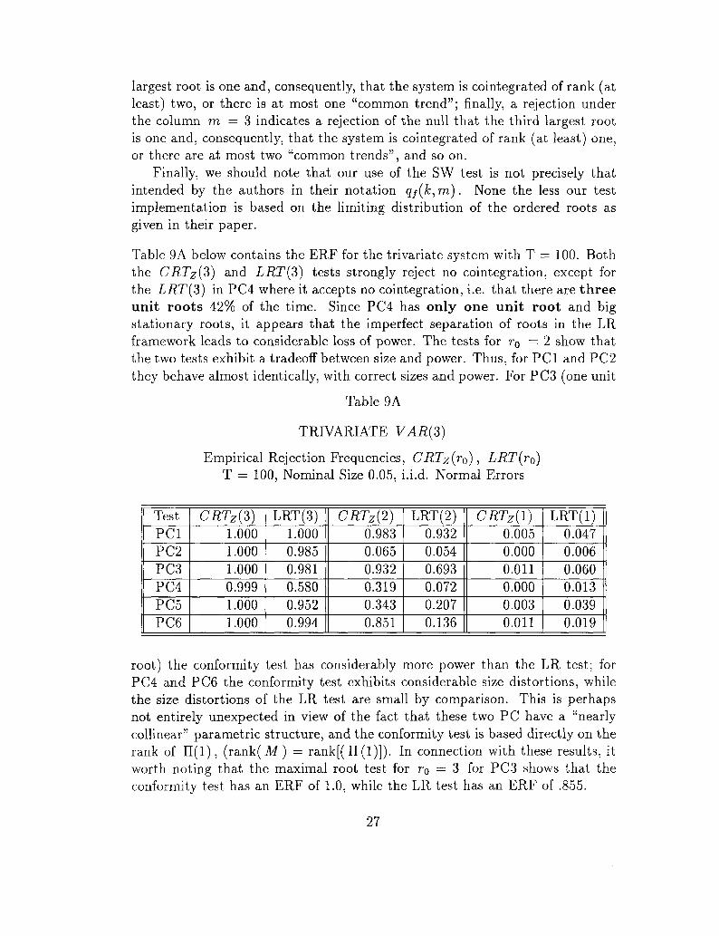
Table 9A below contains the ERF for the trivariate system with T = 100. Boththe CRTz{3) and LRT(3) tests strongly reject no cointegration, except forthe LRT(3) in PC4 where it accepts no cointegration, i.e. that there are threeunit roots 42% of the time. Since PC4 has only one unit root and bigstationary roots, it appears that the imperfect separation of roots in the LRframework leads to considerable loss of power. The tests for r0 = 2 show thatthe two tests exhibit a tradeoff between size and power. Thus, for PCI and PC2they behave almost identically, with correct sizes and power. For PC3 (one unit

Table 9A

TRIVARIATE VAR(3)

Empirical Rejection Frequencies, CRTz(r0), LRT(rQ)T = 100, Nominal Size 0.05, i.i.d. Normal Errors

TestPCIPC2PC3PC4PC5PC6

CRTZ{2)1.0001.0001.0000.9991.0001.000

LRT(3)1.0000.9850.9810.5800.9520.994

CRTZ{2)0.9830.0650.9320.3190.3430.851

LRT(2)0.9320.0540.6930.0720.2070.136

CRTZ{1)0.0050.0000.0110.0000.0030.011

LRT(l)0.0470.0060.0600.0130.0390.019

root) the conformity test has considerably more power than the LR test; forPC4 and PC6 the conformity test exhibits considerable size distortions, whilethe size distortions of the LR test are small by comparison. This is perhapsnot entirely unexpected in view of the fact that these two PC have a "nearlycollinear" parametric structure, and the conformity test is based directly on therank of 11(1), (rank(M) = rank[( II (1)]). In connection with these results, itworth noting that the maximal root test for ro = 3 for PC3 shows that theconformity test has an ERF of 1.0, while the LR test has an ERF of .855.

27

Finally, we observe from the last two columns of the table that both testshave comprable ERF in detecting cointegration, in that the entries of the lastcolumn (which relates to the test that the smallest root of the system is zero)are very close to zero, and comparable as between the two tests.

In Table 9B, below, we give the ERF for the trivariate system when T = 500. Asexpected, the results closely parallel those indicated by the asympotic theory,and the problems encountered with the smaller sample disappear, in all but oneinstance: The CRTz(2) test for the last two roots in PC6 still exhibits a highsize distortion.

The results for SW's qj(ki m) test are given in Table 10 below. They show thatthis test is very weak and inconclusive; it suffers both from power problems andsize distortions. These problems do not seem to disappear when the sample isincreased to T = 500. As an example, for T = 100, PCI (which has one unitroot), the test correctly rejects the hypothesis that the third and second largestroots are one, (for m = 2 and m = 3), but it also rejects the hypothesis that thelargest root is one in 63% of the replications, and thus finds stationarity!

Table 9B

TRIVARIATE VAR(3)

Empirical Rejection Frequencies, CRTz(r0), LRT(r0)T = 500, Nominal Size 0.05, i.i.d. Normal Errors


CRTZ(3)1.0001.0001.0001.0001.0001.000

LRT(3)1.0001.0001.0001.0001.0001.000

CRTZ{2)1.0000.0161.0000.0570.9460.445

LRT(2)1.0000.0501.0000.0710.9850.071

CRTZ{1)0.0010.0000.0020.0000.0020.000

LRT(l)0.0450.0070.0620.0110.0630.007

This problem is incountered among all configurations, and in both samples.As another example, consider PC4 (which has two unit roots) where the testalmost always accepts the null that the third largest root is one, i.e. that thesequence is 7(1) and not cointegrated. By constrast, for T = 100 in 37% ofthe replications it accepts the view that the sequence is stationary, since itrejects the null that the largest root is one. For T = 500 this situation occursin 59% of the replications.

28

Thus, our conclusion has to be that the SW test procedure does not providea reliable guide for empirical research, a conclusion also reached in Yap andReinsel (1995).

Table 10

TRIVARIATE VAR(3)

Empirical Rejection Frequencies for S h W's qj(k:m) testk = 3 , Nominal Size 0.05, i.i.d. Normal Errors

m —>PCIPC2PC3PC4PC5PC6

000000

r

1.637.528.425.377.353.146

r

000000

= IOC2

.995

.377

.086

.006

.172

.013

30.9830.5300.1290.0020.2930.053

T

10.5660.4900.6960.5610.4240.619

r

100000

= 50C2

.000

.354

.953

.593

.383

.173

110000

3.000.000.999.004.996.070

In Tables 11 and 12 we present the results for the quadrivariate model; Table11A reports ERF for the conformity and LR tests for sample size T = 100,Table 11B those for T = 500, while Table 12 contains the results for the SWtests.

Both conformity and LR tests detect cointegration quite well although theconformity test exhibits more power as evident from the first two columns of thetable. The tests for the last 3 roots, columns labeled CRTz{S) and LRT(3),respectively, show the same pattern of trade-off between size and power as wenoted in the trivariate system.

For PCI both tests correctly reject the hypothesis that all four roots are zero.For PC2 CRTZ{3) has considerable power, .95, while the LRT(3) test hasrelatively low power, .587, i.e. in approximately 42% of the replications itaccepts the hypothesis the last three roots are zero, i.e. that the system hasthree unit roots, while in truth PC2 has only two unit roots. On the otherhand for PC3 both tests have size problems; CRTz(3) rejects the hypothesisthat the last three roots are zero in about 50% of the replications, while LRT(3)rejects this hypothesis in about 10% of the replications, even though the nominalsize is 5%. In PC4 and PC5, which both have large stationary roots, we see thatLRT(3) has severe power problems: in about 60% and 70% of the replicationsit accepts the hypothesis that the last three roots are zero, i.e. it accepts the

29

hypothesis that the cointegrating rank is 1, instead of the correct 3 and 2,respectively.

Table 11A

QUADRIVARIATE VAR{4)

Empirical Rejection FrequenciesCRTz(r0), LRT(ro),T = 100

Nominal Size 0.05, i.i.d. Normal Errors

TestPCIPC2PC3PC4PC5PC6PC7PC8

J_TestPCIPC2PC3PC4PC5PC6PC7PC8

CRTZ{4)1.001.001.001.001.001.001.001.00

CRTZ{2)0.7430.0480.0110.1940.1000.2450.0930.146

LRT(4)1.0001.0001.0001.0001.0000.9810.9940.986

LRT(2) |

0.5820.0610.0140.0740.0660.1520.0450.057

CRTZ(3)1.0000.9500.5020.9890.8390.9840.8470.892

CRTZ{\)0.0030.0000.0000.0010.0000.0010.0000.003

LRT(3)0.9430.5870.1050.4000.3180.5680.2600.295

LRT(l) |i

0.0440.0100.0070.0150.0200.0360.0140.022

The CRTz(3) test exhibits very serious size distortions for PC8; in 89% of thereplications it rejects the (true) null that the last three roots are zero. Thecomparable figure for the LRT(3) is 30%, so that it too suffers size distortionsalbeit of a milder nature. For PC7 (which has only two unit roots) CRTz{3)has considerably more power than the LRT(3), since the latter accepts thehypothesis that the cointegrating rank is 1 (q — r0) instead of the correct 2 in74% of the replications. By contrast, the CRTz(3) test does so in only 15% ofthe replications. For the last two roots (columns labeled CRTzi^) , CRTz(l),and similarly for the LR test) we observe relatively low power for both tests

30

even though on balance the conformity tests is the more powerful of the two;the size characteristics are also similar with the LR test having empirical sizesomewhat closer to the nominal one.

Table 11B

QUADRIVARIATE VAR(A)

Empirical Rejection FrequenciesCRTz(r0), LRT{r0), T = 500

Nominal Size 0.05, i.i.d. Normal Errors


Test

PCIPC2PC3PC4PC5PC6PC7PC8

CRTZ(\)1.001.001.001.001.001.001.001.00

CRTZ(2)1.0000.0030.0000.3010.0040.9790.0040.001

LRT(4)1.001.001.001.001.001.001.001.00

LRT(2)

1.0000.0550.0030.7550.0711.0000.0510.011

CRTZ(3)1.0001.0000.0401.0000.8831.0000.9750.096

CRTZ(1)0.0000.0000.0000.0010.0000.0010.0000.000

LRT(3)1.0001.0000.0571.0000.8951.0000.9550.080

LRT(l)

0.0520.0670.0020.0570.0070.0510.0120.053

In addition, it is worth noting that the conformity maximal root test, MRC(2),for the second root has much higher power than the corresponding trace, CRTZ(2),test; as an example for PCI the table entry for the trace test is .743; if werecorded the maximal root test based result it would have been .871. The sameis true of PC4 and PC6. The opposite phenomenon holds for the maximal rootof the LR test, viz. that the power characteristics of the maximal root basedLR test are lower than those of the trace based LR test.

Finally, as before, both tests easily detect the presence of cointegration.

31

The results for T = 500 are given in Table 11B. As expected, both tests now havealmost no size or power problems. It is noteworthy how close the results are onthe tests for the last three roots (upper panel). An anomaly in terms of earlierressults occurs in PC4 (which has one unit root and two large stationary roots),where the conformity test rejects the hypothesis that the last two roots are zeroin 30% of the replications only, while the LR test rejects this hypothesis in 75%of the replications. This is the only case where the CRTz test underestimatesthe true cointegrating rank, a feature, thus far, almost exclusively of the LRTtest. Again, it is worth noting that the maximal root based conformity testin this case has higher power, .504 while the maximal root based LR test hasidentical power as reported in the table, viz. .747.

We conclude this section by examining the results obtained using the SWqf(k,m) test for the quadrivariate system. They are given in Table 12 below.As in the smaller system, we have confusing results here as well. The test's per-formance is very weak and inconclusive: the test correctly detects the presenceof cointegration, by rejecting the null of 4 'common trends', but suffers frompower losses in that it frequently accepts stationarity! In light of these findingsthe intermediate results about the rank are of no significance and thus we mustreiterate our finding that the SW cannot be recommended for use in empiricalapplications.

Table 12

QUADRIVARIATE VAR(±)

Empirical Rejection Frequencies for S & W's qf(k:m) testk = 4 , Nominal Size 0.05, i.i.d. Normal Errors

m —>PCIPC2PC3PC4PC5PC6PC7PC8

00000000

1.879.688.613.512.375.498.332.204

00000000

T =2

.997

.720

.403

.183

.087

.340

.133

.045

100

00000000

3.999.966.615.858.157.223.565.385

00000000

4.996.997.892.999.972.978.998.974

00000000

1.905.656.599.789.465.382.359.221

10000000

2.000.697.349.450.552.997.096.111

500

11

1010010

3.000.000.878.000.366.992.000.531

11111111

4.00.00.00.00.00.00.00.00

32

6.2 Correlated and Non-Symmetric Errors

In this subsection we examine the sensitivity of the tests examined earlier tomisspecification in the error process. In particular we examine "VARs" whoseerror process is a moving average, and a centered chi-square (i.e. Xi ~ 1 • Wepresent, in Tables 13, 14, 15, and 16, results only for the conformity and LRtests. In the trivariate case we deal with PCI, PC2, PC5 and PC6, while in thequadrivariate case we deal with PCI, PC2, PC4, and PC5.

In Tables 13 through 16 we present the ERF for the case where the error processis misspecified. The entries therein, therefore, are not to be interpreted in thesame strict manner as in the earlier tables; in that case the entries serve twoimportant purposes. First, they indicate how closely the critical values obtainedfrom the limiting distribution approximate the finite (small in the case of T =100) critical values and, second, how large should the sample be in order toget a very close approximation. In addition, they also provide information onthe relative performance of the conformity vis-a-vis the likelihood ratio test.In the case where the error processes are misspecified the results shed lightonly on the relative performance of the two tests, except in the case where themisspecified error process yields precisely the same asymptotic theory as thestandard (i.i.d. normal) error process. When we use an MA(3) error processthe limiting distribution of both tests is not the same. In the case of i.i.d.Xi — 1 errors, the latter would yield the same limiting distribution theory andin principle such results should have the same interpretation as in the earliertables.

Table 13A

TRIVARIATE VAR(3)

Empirical Rejection Frequencies, CRTz(r0), LRT(r0)T = 100, Nominal Size 0.05, MA(3) Errors

TestPCIPC2PC5PC6

CRTZ{3)1.001.001.001.00

LRT(3)1.001.001.001.00

CRTZ{2)1.0000.5170.1870.854

LRT(2)1.0000.3270.1550.381

CRTZ(1)0.0130.0030.0040.004

LRT(l)0.0710.0190.0670.016

In Table 13A we have the ERF for T = 100, with the trivariate systemand moving average errors. Both tests always reject the hypothesis of no-cointegration, i.e. r0 = 3, as is evident from the ERF in the first column

33

block of the table. For PCI we see almost no difference relative to the case ofi.i.d. normal errors, see Table 9A, except slight increases in power for r0 = 2,for both tests, and a slight increase in the empirical size of both tests for the lastroot. For PC2 both tests have size problems when testing for the last two roots,rQ = 2; the CRTZ{2) test suffers more with an ERF of 51.7% versus 32.7%for the LRT(2) test. In PC5 both tests have power problems when testing forthe last two roots; now LRT{2) suffers slightly more than CRTZ{2) . For PC6we have again size problems, as in PC2, when testing r0 = 2. The CRTz{2)test has higher size distortion compared to the LRT test. Note that the sizedistortion for the LRT test, for PC6, is almost the same as its size distortion forPC2. Both PC2 and PC6 have two unit roots but they differ in the magnitudeof their stationary roots. Both tests fare equally badly or equally well, except inthe case of PC6 (which has two unit roots and two large stationary roots) wherethe conformity test rejects the null of two zero roots in 85% of the replications,while the likelihood ratio test does so in only 38% of the replications. Finally,both tests have no problem in detecting cointegration, i.e. they almost alwaysaccept that the last root is zero.

The results for T = 500, given in Table 13B below, do not show substantialimprovement, although now the performance of the two tests is equally bad orequally good, depending on one's point of view. For example the poor perfor-mance of the conformity test for PC6 is offset by the uniformly worse perfor-mance of the likelihood ratio test in testing whether the smallest root is zero,which is rejected inordinately frequently by that test.

Table 13B

TRIVARIATE VAR(3)

Empirical Rejection Frequencies, CRTz(r0), LRT(r0)T = 500, Nominal Size 0.05, MA(3) Errors

TestPCIPC2PC5PC6

CRTZ{Z)1.001.001.001.00

LRT(3)1.001.001.001.00

CRTZ{2)1.0000.4770.8740.747

LRT(2)1.0000.5480.9880.415

CRTZ{1)0.0100.0030.0300.001

LRT(l)0.0870.0520.1730.022

The ERF of the two tests for the case of non-symmetric errors is given in Tables14A and 14B below. Here the limiting distribution theory remains valid andthus the results have the same interpretation as those in Tables 10 and 11.

34

Table 14A

TRIVARIATE VAR(3)

Empirical Rejection Frequencies, CRTZ{TQ) , LRT(r0)T = 100, Nominal Size 0.05, x2 Errors

TestPCIPC2PC5PC6

CRTZ(3)1.0001.0001.0000.999

LRT(3)1.0000.9290.8680.562

CRTZ{2)0.9610.0540.1690.654

LRT(2)0.8930.0530.0990.082

CRTz(l)0.0050.0000.0010.005

LRT(l)0.0510.0130.0230.019

Table 14A has results for T = 100 and Table 14B has results for T = 500.For T = 100, the first two columns indicate a superior performance on the

part of the conformity test vis-a-vis the likelihood ratio test. For example inthe case of PC6 (which has two unit roots and one large stationary root) thelikelihood ratio test in 44% of the replications accepts the hypothesis that thesequence is 1(1) and noncointegrated. On the other hand, for the same PC6,CRTZ rejects the hypothesis of two zero roots in 65% of the replications (sizedistortion), while the likelihood ratio test does so in only 8% of the replications.Otherwise the performance of the two tests is comparable. As we noted earlierthe maximal root version of the conformity test has considerably smaller sizedistortion and approximately the same power. Thus, for example, if instead ofthe CRTz(2) (trace) test we used the maximal root test (i.e. used only thesecond root) the ERF would have been .212 for the conformity test and .077 forthe likelihood ratio test. Contrast this with Table 14A where the correspondingentries are .654 and .082, respectively.

Table 14B

TRIVARIATE VAR(3)

Empirical Rejection Frequencies, CRTz(ro), LRT(r0)T = 500, Nominal Size 0.05, x2 Errors

TestPCIPC2PC5PC6

CRTZ(3)1.001.001.001.00

LRT(3)1.001.001.001.00

CRTZ{2)1.0000.0060.3850.543

LRT(2)1.0000.0450.6360.071

CRTZ{1)0.0010.0000.0010.001

LRT(l)0.0530.0040.0540.006

35

The results for T = 500 are given in Table 14B. Again the two tests performequally well, except in PC5 and PC6, when testing the hypothesis that the lasttwo roots are zero. For PC5 the power of the conformity test is .385, whilethat of the likelihood ratio test is .636. As we noted earlier, however, if weemploy tests based on the maximal root the relevant powers would have been.522 and .62, respectively. For PC6, the conformity test rejects a correct nulltoo frequently, in 54% of the replications.

In Table 15A, below, we present the ERF for the quadrivariate system, T =100, and MA(4) errors.

In the first two columns of the table it is evident that the two tests uniformlyreject the hypothesis that the sequence is 1(1) and not cointegrated. In the nexttwo columns the conformity test unformly rejects the hypothesis that there arethree zero roots, i.e. that the system has three unit roots. The likelihoodratio test, however, accepts the hypothesis of three zero roots in 32% of thereplications, i.e. it finds cointegration of rank 1, instead of the correct rank 2.In the next two columns the conformity test exhibits size distortions, i.e. itrejects the correct null of two zero roots in PC2 and PC5 in about 78% of

Table 15 A


Empirical Rejection Frequencies, CRTz(ro), LRT(r0)T = 100, Nominal Size 0.05, MA(4) Errors

TestPCIPC2PC4PC5

Test

PCIPC2PC4PC5

CRTZ{4)1.001.001.001.00

CRTZ{2)1.0000.7851.0000.780

LRT(4)1.001.001.001.00

LRT(2)J1.0000.0580.9990.174

CRTZ(S)1.001.001.001.00

CRTZ{\)0.0060.0010.1320.046

LRT(3)1.0001.0001.0000.685

LRT(l)

0.0530.0040.1610.033

the replications, while the likelihood ratio test does so in aboutthe replications, respectively.

Vo and 17% of

36

Finally, in the tests of the smallest root, both conformity and likelihoodratio tests do equally well, or equally badly, exhibiting size distortions for PC4,i.e. they reject a correct null in 13% and 16% of the replications respectively.

When the sample size is increased to T = 500, the behavior of the coformitytest improves, while that of the likelihood ratio test worsens. None the less sizedistortions persist for the conformity test in the case of PC2 and PC5 and thesize distortion for the likelihood ratio test in PC5 (LRT{2)) worsens.

In Tables 16 A and 16B we presents ERF for the case when the error process isnon-symmetric ( x\ ~ 1 )• For T = 100, the conformity test exhibits considerablymore power than the likelihood ratio test, as evident from the first four columnsof Table 16A. The conformity test exhibits slightly more size distortions thanthe likelihood ratio test, as evident from the third column.

Table 15B


Empirical Rejection Frequencies, CRTz{ro), LRT(r0)T = 500, Nominal Size 0.05, MA(3) Errors

TestPCIPC2PC4PC5

Test

PCIPC2PC4PC5

CRTZ(4)1.001.001.001.00

[_CRTZ(2)

1.0000.5921.0000.476

LRT(4)1.001.001.001.00

LRT(2)

1.0000.0490.9990.197

CRTZ(3)1.001.001.001.00

CRTZ{1)0.0010.0010.0010.002

LRT(3)1.001.001.001.00

LRT(l)

0.0510.0070.0960.013

As we also noted in the trivariate system, the power characteristics of the con-formity test is improved if we use, instead of the trace, the maximal root test.Thus, as an example, for PCI and the test that the last two roots are null, themaximal root test will yield an ERF of .816, instead of .685, as recorded in thetable.

The use of the larger sample size, T = 500, improves the performance ofboth tests, but the likelihood ratio test imrpoves more significantly. The twotests perform equally well in testing whether all four roots, the last three roots,

37

Table 16 A


Empirical Rejection Frequencies, CRTz(ro), LRT(r0)T = 100, Nominal Size 0.05, x2 Errors

TestPCIPC2PC4PC5

| Test

PCIPC2PC4PC5

CRTZ(4)1.001.001.001.00

CRTZ(2)0.6850.0430.1730.062

LRT(4)0.9990.9990.9750.955

LRT(2)j

0.5480.0630.0880.055

CRTZ(3)1.0000.9810.9990.749

ICRTZ(1)0.0010.0010.0010.001

LRT(3)0.9310.7200.4220.259

LRT(l)

0.0410.0100.0270.019

Table 16B


Empirical Rejection Frequencies, CRTz(r0), LRT(r0)T = 500, Nominal Size 0.05, x2 Errors

TestPCIPC2PC4PC5

Test

PCIPC2PC4PC5

CRTZ(4)1.001.001.001.00

CRTZ(2)1.0000.0010.2000.004

LRT(4)1.001.001.001.00

CRTZ(3)1.0001.0001.0000.783

LRT(2)J| CRTZ(1)1.0000.0490.7100.073

0.0010.0010.0010.001

LRT(3)1.0001.0001.0000.811

LRT(l)

0.0510.0100.0400.016

or the last root, are null; in the test of whether the last two roots are null, i.e.

38

that the system has two unit roots (when in fact it has only one) the conformitytest has low power relative to that of the likelihood ratio test, .2 as against .71.

We should note gain that the maximal root version of the conformity test ex-hibits somewhat greater power. As an example, if we employ the maximal rootto test the hypothesis that the last three roots are zero for PC5 (which in facthas only two zero roots) the ERF would have been .902, instead of .783 asrecorded in Table 16B. Similarly, for PC4 the maximal root test has an ERF of.380, instead of .200 as is recorded in Table 16B.

We conclude the discussion of the performance of the conformity test basedon zero root estimators by examining the case of trivariate random walk anda 10-variate VAR{2), of cointegrating rank nine and eight, i.e. with one andtwo unit roots, respectively. The first is designed to guage the performanceof the conformity and likelihood ratio tests when the underlying sequence is7(1) and not cointegrated, and the second to examine the cojecture that inreltively small samples the likelihood ratio test will do relatively less well in largesystems, especially when the test pertains to the smaller roots of the system.Due to computatinal limitation we did not undertake a full examination of suchstructures, but Tables 17, 18, and 19 are all based on 3,500 replications. Theconstruction of the vector random walk is self evident. In the 10-variate systemthe stationary roots were, respectively, .6, .55, .5, .45, .4, .35, .3, .26, .22, .19,.17, .14, .12, .09, . 07, .06, .04, .02 and .6, .55, .5, .45, .4, .35, .3, .26, .22, .19,.17, .14, .12, .09, . 07, .06, .04. Table 17, contains the results for the trivariaterandom walk, and Tables 18 and 19 those for the 10-variate system.

Table 17

TRIVARIATE VECTOR RANDOM WALK

ERF, Trace and Maximal Root TestsVarious Samples, Nominal Size 0.05, normal errors (i.i.d.)

T |

100150200300500

CRTZ{?>)

0.07710.07290.07290.06060.0589

LRT(3) 1| MRC(S)0.03030.03940.04770.04460.0509

0.08030.07540.06800.05800.0571

MRT(3) [0.02310.03260.03910.04200.0460

From Table 17 is quite evident that the two procedures perform equally well.

39

Table 18

10-VARIATE VAR{2), Cointegrated of rank 9

ERF, Trace and Maximal Root TestsNominal Size 0.05, normal errors (i.i.d.)

II ||

J r0 || CRTZ

10987654321

1.0001.0001.0001.0000.9990.7370.0630.0000.0000.000

T =LRTJ

0.9910.9770.9440.8780.8040.6740.5100.3120.1310.031

= 75[ MRC

1.0001.0001.0001.0000.9980.8360.2440.0060.0000.000

MRT

0.0000.0000.0000.0000.0010.0020.0090.0270.0920.031

1CRTZ

1.0001.0001.0001.0001.0000.9560.2780.0020.0000.000

T =

LRT

1.0001.0001.0001.0000.9990.9960.9790.8640.4810.040

100

MRC1.0001.0001.0001.0000.9990.9540.4710.0330.0000.000

MRT

0.2400.1100.0920.1060.1440.1800.2800.3490.5070.040

Table 19

10-VARIATE VAR(2), Cointegrated of rank 8

ERF, Trace and Maximal Root TestsNominal Size 0.05, normal errors (i.i.d.)

To

10987654321

CRTZ

1.0001.0001.0001.0000.9980.7110.0490.0000.0000.000

T =

LRT

0.984[ 0.936

0.8560.7290.5830.3860.2060.0650.0120.008

= 75

MRC1.0001.0001.0001.0000.9980.8680.3110.0130.0000.000

MRT

0.0000.0000.0000.0000.0000.0030.0060.0140.011

L0.008

CRTZ

1.0001.0001.0001.0001.0000.9170.1470.0000.0000.000

T =

LRT

1.0001.0001.0000.9980.9900.9330.7110.2390.0310.009

100

MRC1.0001.0001.0001.0001.0000.9660.5670.0560.0000.000

MRT

0.3340.1540.0970.0910.1040.1420.1960.2350.0230.009

40

The conformity test has a tendency toward positive size distortions, whilethe likelihood ratio test has a tendency toward negative size distortions. Inthe case of the latter case one sees the strong influence exerted by the impositionof the (false) null. One might argue that, at least in the case of the likelihoodratio test these (trace) tests are moot since, under the null (that all three rootsare zero) the undelying sequence is not cointegrated and, thus, it violates abasic assumption involved in estimation.

6.3 Performance of the Standard CCT Tests

In Tables 20A and 20B we give the empirical rejection frequencies for the "stan-dard" conformity tests; these tests involve hypotheses regarding the sum ofroots, at least one of which is nonnull. In such cases we have a well devel-oped asymptotic theory, and the results presented therein indicate considerablepower, both for the trivariate and the quadrivariate design. Notice that herewe actually test hypotheses that the sum is not null by means of confidenceintervals. For simplicity of comparison with the earlier results we report ourfindings as if the hypotheses asserted that the sum of the roots in question werenull, when in fact we know, from the design that they are not. Thus, althoughthe tables read as if they report on the rejection of a false null, in fact theyreport on the acceptance of a true null.

Table 20A

TRIVARIATE VAR(3)Empirical Rejection Frequencies for CCT and CRT Tests.

Test

CCTCRT(2)CRT(l)

CCTCRT(2)CRT(l)

PCI

i

1l

N

0000A.

0000A.

PC2

1NN

1NN

00A.A.

00A.A.

T0

T

PC3

: 100

.99931

N

11

N

00A.

0

: 500

0000A.

PC4

.9993NN

1NN

A.A.

.00A.A.

PC5

1 000.9923

N

11

N

A.

0000A.

PC6

0.9996NN

1NN

A.A.

.00A.A.

41

Table 20B

QUADRIVARIATE VAR(4)Empirical Rejection Frequencies for CCT and CRT Tests.

|_ Test

1CCT

CRT(3)CRT(2)CRT(l)

CCTCRT(3)CRT(2)CRT(l)

PCI

111

N

111

|_N

.00

.00

.00

.A.

.00

.00

.00

.A.

PC2

11

NN

11

NN

.00

.00

.A.

.A.

.00

.00

.A.

.A.

PC3r

1.00N.A.N.A.N.A.

r

1.00N.A.N.A.N.A.

PC4 PC5

r = IOO0.9997

1.000.9983

N.A.

0.99970.9993

N.A.N.A.

r = 5001.001.001.00

I N.A.

1.001.00

N.A.N.A.

PC6

111

N

111

N

.00

.00

.00

.A.

.00

.00

.00

.A.

PC7

1.000.9993

N.A.N.A.

1.001.00

N.A.N.A.

PC8

1NNN

1NNN

.00

.A.

.A.

.A.

.00

.A.

.A.

.A.

7 Conclusions

The present study explores the properties of three system-based cointegrationtests: the newly proposed Conformity Test for Cointegration, Dhrymes (1996b),the likelihood ratio test, Johansen (1988), (1991), and Stock and Watson'sqf(k, m) test, Stock and Watson (1988). The main contribution of the paper isa detailed study of the finite sample properties of these tests.

In carrying out this study we have employed a new method for the design ofthe data generating process, (DGP), here a cointegrated VAR(n), that allows usto specify the characterisitc roots of the system at will. Computational problemsconfined our full scale analysis, at most, to a quadrivariate VAR(4) with one,two and three unit roots, and stationary roots which were alternatively small,medium, and large (up to .95); there was also a limited examinatin of trivariaterandom walks and 10-variate systems with one and two unit roots only. Theprocedure for obtaining such parametric specifications is outlined in Dhrymes(1996a).

The DGP we have actually employed were two VARs with coefficient ma-trices which are unconstrained beyond the specification of the system's roots;in particular we have employed VARs with three variables and three lags, andfour variables and four lags, and we have used two sample sizes, 100 and 500.The first sample size is used widely in other Monte Carlo studies of this sort,

42

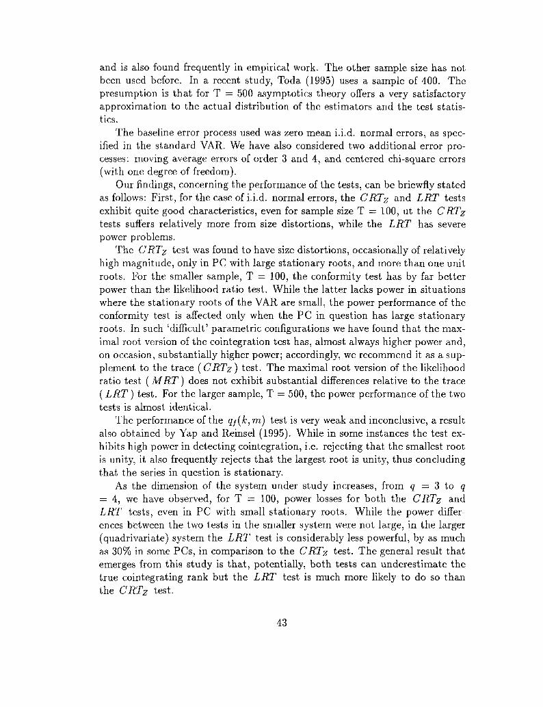
and is also found frequently in empirical work. The other sample size has notbeen used before. In a recent study, Toda (1995) uses a sample of 400. Thepresumption is that for T = 500 asymptotics theory offers a very satisfactoryapproximation to the actual distribution of the estimators and the test statis-tics.

The baseline error process used was zero mean i.i.d. normal errors, as spec-ified in the standard VAR. We have also considered two additional error pro-cesses: moving average errors of order 3 and 4, and centered chi-square errors(with one degree of freedom).

Our findings, concerning the performance of the tests, can be briewfly statedas follows: First, for the case of i.i.d. normal errors, the CRTz and LRT testsexhibit quite good characteristics, even for sample size T = 100, ut the CRTztests suffers relatively more from size distortions, while the LRT has severepower problems.

The CRTz test was found to have size distortions, occasionally of relativelyhigh magnitude, only in PC with large stationary roots, and more than one unitroots. For the smaller sample, T = 100, the conformity test has by far betterpower than the likelihood ratio test. While the latter lacks power in situationswhere the stationary roots of the VAR are small, the power performance of theconformity test is affected only when the PC in question has large stationaryroots. In such 'difficult' parametric configurations we have found that the max-imal root version of the cointegration test has, almost always higher power and,on occasion, substantially higher power; accordingly, we recommend it as a sup-plement to the trace (CRTz) test. The maximal root version of the likelihoodratio test (MRT) does not exhibit substantial differences relative to the trace(LRT) test. For the larger sample, T = 500, the power performance of the twotests is almost identical.

The performance of the q/(k, m) test is very weak and inconclusive, a resultalso obtained by Yap and Reinsel (1995). While in some instances the test ex-hibits high power in detecting cointegration, i.e. rejecting that the smallest rootis unity, it also frequently rejects that the largest root is unity, thus concludingthat the series in question is stationary.

As the dimension of the system under study increases, from q — 3 to q= 4, we have observed, for T = 100, power losses for both the CRTz andLRT tests, even in PC with small stationary roots. While the power differ-ences between the two tests in the smaller system were not large, in the larger(quadrivariate) system the LRT test is considerably less powerful, by as muchas 30% in some PCs, in comparison to the CRTz test. The general result thatemerges from this study is that, potentially, both tests can underestimate thetrue cointegrating rank but the LRT test is much more likely to do so thanthe CRTZ test.

43

When moving average errors were used as the error process in the DGP wehave observed increased power at some instances; this may be attributable tothe overestimation of the non-zero roots in both the CRTz and LRT. Butthe size distortions are now much more severe for both tests. An importantand interesting finding in this case is that as the sample size increases thesize distortions for the LRT test increase rather than decrease, se for exampleTables 13A and 13B, thus making the use of the LRT test especially susceptibleto error.

On the other hand, when non-symmetric \2 errors are used we have ob-served no size problems, as in the case of i.i.d. normal errors. Loss of power wasobserved but it was limited to the case of 'difficult' PC, with large stationaryroots and in general disappear when a sample of T = 500 was used.

The two finding regarding alternative error processes are easily understoodif we note that with MA(3) or MA(4) errors the estimation procedure employedrenders the asymptotic theory on which the tests are based invalid. Thus, theempirical performance of the tests need not improve with an increase in samplesize. On the other hand, the asymptotic theory on which the tests are basedremains valid when the error process is i.i.d. with distribution Xi ~~ 1 •

The conformity test based on the nonzero roots, which has a standard limit-ing distribution, is extremely effective in establishing the presence of cointegra-tion, but is not easily employed in establishing the rank of cointegration. Thisis due to the fact that it lacks power against alternatives that involve sums ofzero roots.

In view of the above we conclude that much better inference is to be ob-tained by the simultaneous use of the CRTz a n d the LRT tests. Their designdifferences should allow a researcher to better capture the probabilistic proper-ties of the series under study. Once cointegration has been established, whichboth tests achieve without any difficulty, the search for the cointegrating rankshould be done using both procedures; LRT is likely to underestimate therank, as Toda (1995) also reports, due to power problems, and the CRTz testcan readily help in reducing this potential. Finally, based on our results, andin agreement with Yap and Reinsel (1995), we cannot recommend the qj(k,m)test for empirical use.

One last comment on the behavior of the the likelihood ratio test. Thistest is effectively based on statistics which reflect the cointegration hypothesis,i.e. the residual matrices V and W employed in such test reflect the rankfactorization BY' imposed by the null. When the null is true this leads to anet benefit for LRT, but when it is false, it seems to result in apreciable lossof power. This seems to be what comes through a great deal of the Monte Carloresults presented earlier. In this light, and whith relatively small samples, theuse of the Conformity test in empirical research seems to be highly desirable.

44

Our work can be extended to several directions. A major field for extensionswould be misspesification analysis: Using the design adopted by this study, wecan test for the effects of lag misspecification in cointegrated VAR(n) models,with n arbitrary. According to the results of Boswijk and Frances (1992), forthe LRT test, underspecification leads to size distortions whereas overspecifi-cation leads to power loss; one can examine this issue in the context of theconformity test.

Given our results on the models with moving average errors, one can extendthe results of Van Giersbergen (1996) on the use of bootstrapping, which canbe applied to the conformity framework. Finally, one can consider the effects ofthe presence or absence of trends in the data and estimation and examine theimpact of such circumstances on the performance of the various tests examinedherein.

45

REFERENCES

Ahn, S.K. and G.C. Reinsel (1990), "Estimation for partially non-stationarymultivariate autoregressive models", Journal of the American Statistical Asso-ciation, vol. 85, pp. 813-823.

Andrews, D.W.K. (1991), "Heteroscedasticity and autocorrelation consistentcovariance matrix estimation", Econometrica, vol. 59, pp. 817-858.

Banerjee, A., J.J. Dolado, D.F. Hendry and G.W. Smith (1986), "Exploringequilibrium relationships in econometrics through static models: Some MonteCarlo evidence", Oxford Bulletin of Economics and Statistics, vol. 48, pp. 253-277.

Blangiewicz, M. and W. Charemza (1990), "Cointegation in small samples; em-pirical percentiles, drifting moments and customized testing", Oxford Bulletinof Economics and Statistics, vol. 52, pp. 303-315.

Bewley R. and M. Yang (1995), "Tests for Cointegration Based on CanonicalCorrelation Analysis", Journal of the American Statistical Association, vol. 90,pp. 990-996.

Boswijk, H.P. (1994), "Testing for an Unstable Root in Conditional and Struc-tural Error Correction Models", Journal of Econometrics, vol. 63, pp. 37-60.

Boswijk, H.P. and Ph.H. Frances (1992), "Dynamic Specification and Cointe-gration", Oxford Bulletin of Economics and Statistics, vol. 55, pp. 313-328.

Cheung, Y. and K.S. Lai (1993), "Finite Sample Sizes of Johansen's LikelihoodRatio Tests for Cointegration", Oxford Bulletin of Economics and Statistics,vol. 55, pp. 313-328.

Dhrymes, P.J. (1984), it Mathematics for Econometrics, second edition, NewYork: Springer-Verlag.

Dhrymes, P.J. (1989), Topics in Advanced Econometrics: vol. I, ProbabilityFoundations, New York: Springer-Verlag.

Dhrymes, P.J. (1996a), "The Design of Monte Carlo Experiments in VAR Sys-tems", Department of Economics, Columbia University Discussion Paper No.9596-14.

Dhrymes, P.J. (1996b), "A Conformity Test for Cointegration", Department ofEconomics, Columbia University Discussion Paper, No. 9696-04.

Dhrymes, P.J. (1998), Time Series, Unit Roots and Cointegration, New York:Academic Press.

46

Dickey, D.A. and W.A. Fuller (1979), "Distribution of the Estimators for Au-toregressive Time Series with a Unit Root", Journal of the American StatisticalAssociation, vol. 74, pp. 420-431.

Dickey, D.A. and W.A. Fuller (1981), "Likelihood Ratio Test Statistics for Au-toregressive Time Series with a Unit Root", Econometrica, vol. 49, pp. 1057-1072.

Engle, R.F. and C.W.J. Granger (1987), "Cointegration and Error Correction:Representation, Estimation and Testing", Econometrica, vol. 55, pp. 251-276.

Giersbergen van, N.P.A. (1996), "Bootstraping the Trace Statistic in VAR mod-els: Monte Carlo Results and Applications", Oxford Bulletin of Economics andStatistics, vol. 58, pp. 391-408.

Haug, A. (1993), "Residual Based Tests for Cointegration: A Monte CarloStudy of Size Distortions", Economics Letters, vol. 41, pp. 345-351.

Haug, A. (1996), "Cointegration Tests, a Monte Carlo Comparison", Journalof Econometrics, vol. 71, pp. 89-115.

Hooker, M.A. (1993), "Testing for Cointegration: Power versus Frequency ofObservation", Economics Letters, vol. 41, pp. 359-362.

Johansen, S. (1988), "Statistical Analysis of Cointegrating Vectors", Journal ofEconomic Dynamics and Control, vol. 12, pp. 231-254.

Johansen, S. (1991), "Estimation and Hypothesis Testing of Cointegration Vec-tors in Gaussian Vector Autoregressive Models", Econometrica, vol. 59, pp.1551-1580.

Johansen, S. and K. Juselius (1990), "Maximum Likelihood Estimation andInference on Cointegration with an Application to the Demand for Money",Oxford Bulletin of Economics and Statistics, vol. 52, pp. 169-210.

Kleinbergen, F. and K. van Dijik (1994), "Direct Cointegration Testing in ErrorCorrection Models", Journal of Econometrics, vol. 63, pp. 61-103.

Kremers, J.J.M., N.R. Ericsson, and J.J. Dolado (1992), "The Power of Coin-tegration Tests", Oxford Bulletin of Economics and Statistics, vol. 54, pp.159-178.

Osterwald-Lenum, M. (1992), "A Note with Quantiles of the Asymptotic Distri-bution of the Maximum Likelihood Cointegration Rank Test Statistics", OxfordBulletin of Economics and Statistics, vol. 54, pp. 461-471.

Phillips, P.C.B. (1991), "Optimal Inference In Cointegrated Systems", Econo-

47

metrica, vol. 59, pp. 283-306.

Phillips, P.C.B. and S. Ouliaris (1988), "Testing for Cointegration Using Prin-cipal Components Methods", Journal of Economic Dynamics and Control, vol.12, pp. 205-230.

Phillips, P.C.B and S. Ouliaris (1990), "Asymptotic Properties of ResidualBased Tests for Cointegration", Econometrica, vol. 58, pp. 165-193.

Reinsel, G.C. and S.K. Ahn (1992), "Vector Autoregressive Models with UnitRoots and Reduced Rank Structure: Estimation, Likelihood Ratio Tests andForecasting", Journal of Time Series Analysis, vol. 13, pp. 355-375.

Saikkonen, P. (1992), "Estimation and Testing of Cointegrated Systems by anAutoregressive Approximation", Econometric Theory, vol. 8, pp. 1-27.

Shin, Y. (1994), "A Residual Based Test of the Null of Cointegration againstthe Alternative of no Cointegration", Econometric Theory, vol. 10, pp. 91-115.

Stock, J. and M. Watson (1988), "Testing for Common Trends", Journal of theAmerican Statistical Association, vol. 83, pp. 1097-1107.

Toda, H. (1995), "Finite Sample Performance of Likelihood Ratio Tests forCointegrating Ranks in Vector Autoregressions", Econometric Theory, vol. 11no. 5 pp. 1015-1032.

Yap, S.F. and G.C. Reinsel (1995), "Estimation and Testing for Unit Rootsin a Partially Non-Stationary Vector Autoregressive Moving Average Model",Journal of the American Statistical Association, vol. 90, pp. 253-267.

48

APPENDIX

In this appendix we present in tabular form a number of results from ourstudy which we did not include in the main body of the paper and on which wedid not offer sustained comment.

Table Al

TRIVARIATE VAR(3)

T =ERF, MRC(r0), MRT(r0)

100, Nominal Size 0.05, normal errors (i.i.d.)


MRC(3)1.001.001.001.001.001.00

MRT(3)0.990.990.850.550.950.99

MRC(2)0.990.110.950.370.400.87

MRT(2)0.930.050.670.060.170.12

MRC{\)0.010.000.010.000.000.01

MRT(l)0.050.010.060.01

L 0.040.02

Table A2

TRIVARIATE VAR(3)

ERF, MRC(r0), MRT(r0)T = 500, Nominal Size 0.05, normal errors (i.i.d.)


MRC(3)1.001.001.001.001.001.00

MRT(3)1.001.001.001.001.001.00

MRC{2)1.000.021.000.070.980.49

MRT(2)1.000.051.000.060.980.07

MRC(1)0.000.010.000.000.020.00

MRT(l)0.050.010.060.010.060.01

49

T =

Table A3

TRIVARIATE VAR(3)

ERF, MRC(r0), MRT(r0)100, Nominal Size 0.05, MA(3) Errors

TestPCIPC2PC5PC6

MRC(3)1.001.001.001.00

MRT(3)1.001.001.001.00

MRC{2)1.000.570.210.87

MRT(2)1.000.320.100.37

MRC(l)0.010.000.040.04

MRT(l)0.070.020.070.02

Table A4

TRIVARIATE VAR(3)

ERF, MRC(r0), MRT(r0)T = 500, Nominal Size 0.05, MA(3) Errors

TestPCIPC2PC5PC6

MRC{3)1.001.001.001.00

MRT(3)1.001.001.001.00

MRC{2)1.000.540.950.77

MRT(2)1.000.530.980.41

MRC{\)0.010.030.030.00

MRT(l)0.090.050.170.02

T =

Table A5

TRIVARIATE VAR(3)

ERF, MRC{r0), MRT{r0)100, Nominal Size 0.05, x2 Errors

TestPCIPC2PC5PC6

MRC(3)1.001.001.000.99

MRT(3)0.990.960.890.47

MRC(2)0.980.080.210.71

MRT(2)0.890.040.080.06

MRC(1)0.000.000.000.00

MRT(l)0.050.010.020.02

50

Table A6

TRIVARIATE VAR(3)

ERF, MRC{r0), MRT(r0)T = 500, Nominal Size 0.05, chi2 Errors

TestPCIPC2PC5PC6

MRC{3)1.001.001.001.00

MRT(3)1.001.001.001.00

MRC(2)1.000.020.520.59

MRT(2)1.000.040.620.06

MRC{1)0.000.000.000.00

MRT(l)0.050.000.050.00

Table A7


ERF, MRC{r0), MRT{r0), T = 100Nominal Size 0.05, normal errors (i.i.d.)


Test


MRC{4)1.001.001.001.001.001.001.001.00

MRC{2)0.870.090.030.270.160.350.150.21

MRT(4)1.001.001.001.001.000.900.990.99

MRT(2)

0.560.050.010.060.050.120.030.04

MRC{3)0.990.970.580.990.860.980.870.90

MRC{\)0.000.000.000.000.000.000.000.00

MRT(3)0.700.590.090.280.210.330.180.20

MRT(l)

0.040.010.000.010.020.040.010.02

51

Table A8


ERF, MRC(r0), MRT(r0), T = 500Nominal Size 0.05, normal errors (i.i.d.)


Test


MRC{i)1.001.001.001.001.001.001.001.00

MRC(2)

1.000.100.000.510.021.000.020.00

MRT(4)1.001.001.001.001.001.001.001.00

MRC(3)1.001.000.081.000.961.001.000.15

MRT(2) || MRC{\)

1.000.050.000.750.061.000.040.00

0.000.000.000.000.000.000.000.00

MRT(3)1.001.000.051.000.921.000.980.07

MRT(l) |!

0.050.000.000.060.070.050.010.00

52

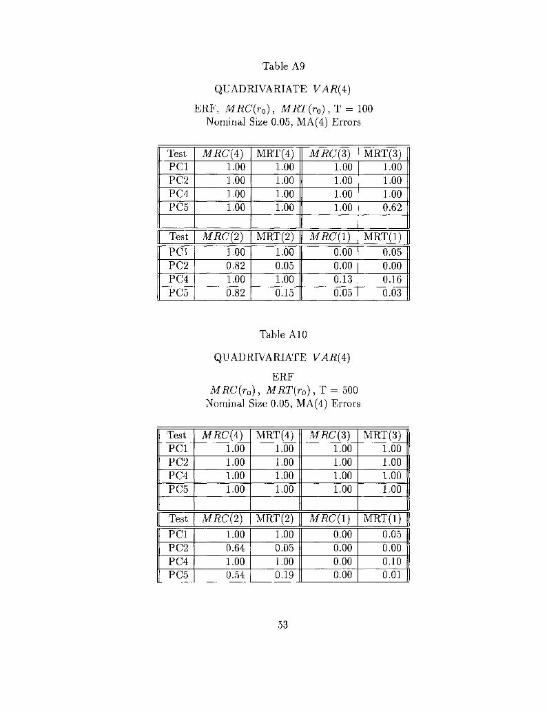
Table A9


ERF, MRC{r0), MRT(r0), T = 100Nominal Size 0.05, MA(4) Errors

TestPCIPC2PC4PC5

| Test

PCIPC2PC4PC5

MRC(i)1.001.001.001.00

MRC{2)

1.000.821.000.82

MRT(4)1.001.001.001.00

MRC(3)1.001.001.001.00

MRT(2) || MRC(1)

1.000.051.000.15

0.000.000.130.05

MRT(3)1.001.001.000.62

MRT(l)

0.050.000.160.03

Table A10


ERFMRC{r0), MRT(r0), T = 500

Nominal Size 0.05, MA(4) Errors

TestPCIPC2PC4PC5

Test

PCIPC2PC4PC5

MRC(i)1.001.001.001.00

MRC{2)

1.000.641.000.54

MRT(4)1.001.001.001.00

MRC{3)1.001.001.001.00

MRT(2)]_Mi2C(l)1.000.051.000.19

0.000.000.000.00

MRT(3)1.001.001.001.00

MRT(l)

0.050.000.100.01

53

Table All


ERF, MRC(r0), MRT(r0), T = 100Nominal Size 0.05, %2 Errors

TestPCIPC2PC4PC5

]_Test

PCIPC2PC4PC5

MRC(4:)1.001.001.001.00

MRC(2)

0.810.080.240.11

MRT(4)0.971.000.940.95

MRT(2)

0.520.050.060.04

MRC(3)1.001.001.000.78

MRC(1)

0.000.000.010.00

MRT(3)0.680.740.300.16

MRT(l)

0.040.010.030.02

Table A12

QUADRIVARIATE VAR{A)

ERF, MRC(r0), MRT(r0), T = 500Nominal Size 0.05, x2 Errors

TestPCIPC2PC4PC5

Test

PCIPC2PC4PC5

ATRC(4)1.001.001.001.00

MRC{2)

1.000.000.380.01

MRT(4)1.001.001.001.00

MRT(2)

1.000.050.720.06

MRC(3)1.001.001.000.90

MRC{1)

0.000.000.000.00

MRT(3)1.001.001.000.85

MRT(l)

0.050.010.050.02

54

1997-1998 Discussion Paper Series

Department of EconomicsColumbia University

1022 International Affairs Bldg.420 West 118th Street

New York, N.Y., 10027

The following papers are published in the 1997-98 Columbia University Discussion Paper serieswhich runs from early November to October 31 of the following year (Academic Year).

The following is a website address where viewers may download some discussion papers. It isa project that is in progress, and therefore the site may not contain all recent working papers.

http: //www. Columbia. edu/dlc/wp/econ/index. html.

For Ordering Hardcopies:

Domestic orders for discussion papers are available for purchase at the cost of $8.00(U.S.) Per paper and $140.00 (US) for the series.

Foreign orders cost $10.00 (US) per paper and $185.00 for the series.

To order discussion papers, please write to the Discussion Paper Coordinator at the aboveaddress along with a check for the appropriate amount, made payable to Department ofEconomics, Columbia University. Please be sure to include the series number of the requestedpaper when you place an order.

1997-98 Discussion PapersEconomics Department, Columbia University

Series no.9798-01

9798-02

9798-03

9798-04

9798-05

9798-06

9798-07

9798-08

TitleOptimal Regulatory Transparency

Russia's Market Transition: Who Has Lost and How?

The Wage Arrears Crisis in Russia

Taxes Versus Legal Rules as Instruments for Equity

Enforcement by Hearing: An Integrated Model of Evidence Production (first draft: 12/95)

Evidence Production, Adversarial Process and the Private Instigation of Suits (first draft:12/95)Structural VAR, MARMA and Open Economy Models

Small Sample Properties of Certain Cointegration Test Statistics: A Monte Carlo Study (Revd.from 7/96)

AuthorsHerk, L.F.

Desai, P.Idson, T.Desai, P.Idson, T.Sanchirico, C.W.

Sanchirico, C.W.

Sanchirico, C.W.

Dhrymes, P.J.Thomakos, D.Dhrymes, P.J.Thomakos, D.

Page 1

Documents

Small Sample Properties of Certain Cointegration Test