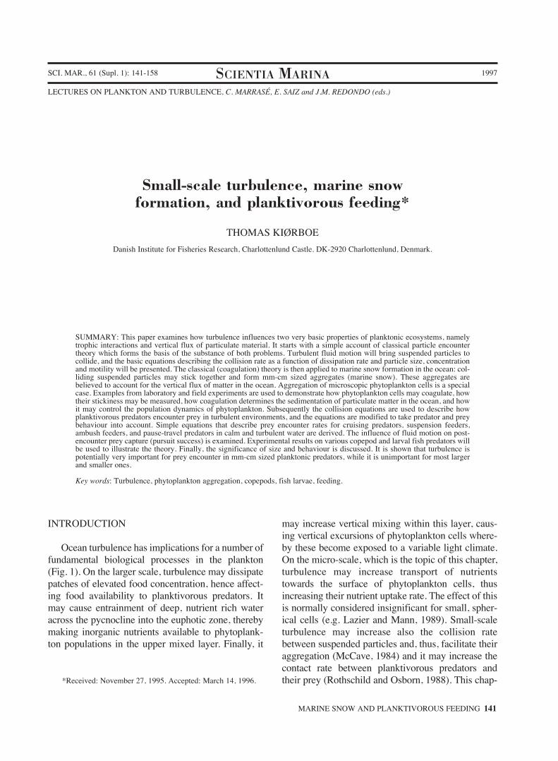
INTRODUCTION

Ocean turbulence has implications for a number offundamental biological processes in the plankton(Fig. 1). On the larger scale, turbulence may dissipatepatches of elevated food concentration, hence affect-ing food availability to planktivorous predators. Itmay cause entrainment of deep, nutrient rich wateracross the pycnocline into the euphotic zone, therebymaking inorganic nutrients available to phytoplank-ton populations in the upper mixed layer. Finally, it

may increase vertical mixing within this layer, caus-ing vertical excursions of phytoplankton cells where-by these become exposed to a variable light climate.On the micro-scale, which is the topic of this chapter,turbulence may increase transport of nutrientstowards the surface of phytoplankton cells, thusincreasing their nutrient uptake rate. The effect of thisis normally considered insignificant for small, spher-ical cells (e.g. Lazier and Mann, 1989). Small-scaleturbulence may increase also the collision ratebetween suspended particles and, thus, facilitate theiraggregation (McCave, 1984) and it may increase thecontact rate between planktivorous predators andtheir prey (Rothschild and Osborn, 1988). This chap-

MARINE SNOW AND PLANKTIVOROUS FEEDING 141

SCI. MAR., 61 (Supl. 1): 141-158 SCIENTIA MARINA 1997

LECTURES ON PLANKTON AND TURBULENCE, C. MARRASÉ, E. SAIZ and J.M. REDONDO (eds.)

Small-scale turbulence, marine snowformation, and planktivorous feeding*

THOMAS KIØRBOE

Danish Institute for Fisheries Research, Charlottenlund Castle. DK-2920 Charlottenlund, Denmark.

SUMMARY: This paper examines how turbulence influences two very basic properties of planktonic ecosystems, namelytrophic interactions and vertical flux of particulate material. It starts with a simple account of classical particle encountertheory which forms the basis of the substance of both problems. Turbulent fluid motion will bring suspended particles tocollide, and the basic equations describing the collision rate as a function of dissipation rate and particle size, concentrationand motility will be presented. The classical (coagulation) theory is then applied to marine snow formation in the ocean: col-liding suspended particles may stick together and form mm-cm sized aggregates (marine snow). These aggregates arebelieved to account for the vertical flux of matter in the ocean. Aggregation of microscopic phytoplankton cells is a specialcase. Examples from laboratory and field experiments are used to demonstrate how phytoplankton cells may coagulate, howtheir stickiness may be measured, how coagulation determines the sedimentation of particulate matter in the ocean, and howit may control the population dynamics of phytoplankton. Subsequently the collision equations are used to describe howplanktivorous predators encounter prey in turbulent environments, and the equations are modified to take predator and preybehaviour into account. Simple equations that describe prey encounter rates for cruising predators, suspension feeders,ambush feeders, and pause-travel predators in calm and turbulent water are derived. The influence of fluid motion on post-encounter prey capture (pursuit success) is examined. Experimental results on various copepod and larval fish predators willbe used to illustrate the theory. Finally, the significance of size and behaviour is discussed. It is shown that turbulence ispotentially very important for prey encounter in mm-cm sized planktonic predators, while it is unimportant for most largerand smaller ones.

Key words: Turbulence, phytoplankton aggregation, copepods, fish larvae, feeding.

*Received: November 27, 1995. Accepted: March 14, 1996.

ter particularly examines the effects of small-scaleturbulence on (i) particle aggregation, especiallyaggregation of phytoplankton cells, and its implica-tions for vertical flux in the ocean and for the dynam-ics of phytoplankton populations, and (ii) planktivo-rous feeding. The core of both of these issues is thatparticles need come into contact (collide) for some-thing to happen. Contact or encounter with prey is aprerequisite for planktivorous feeding; and collisionsbetween suspended particles (such as phytoplanktoncells) is a prerequisite for particles to combine intoaggregates. Small-scale turbulence increases the rateat which this happens.

The encounter rate, E (# of encounters per unittime and unit volume), between two types of sus-pended particles, occurring at concentrations Ca andCb, can be written as:

E = βCaCb (1)

where β is the encounter rate kernel. β has dimen-sions of volume per unit time (L3T-1) and is a func-tion of the size and motility of the particles and of

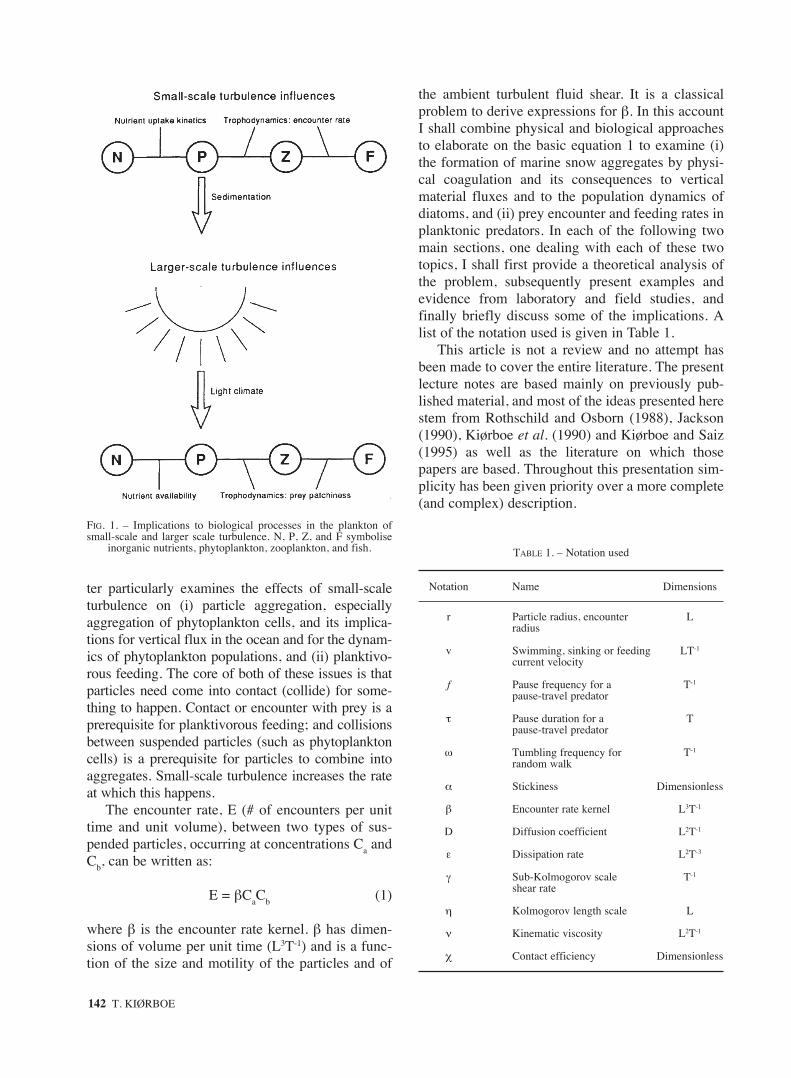
the ambient turbulent fluid shear. It is a classicalproblem to derive expressions for β. In this accountI shall combine physical and biological approachesto elaborate on the basic equation 1 to examine (i)the formation of marine snow aggregates by physi-cal coagulation and its consequences to verticalmaterial fluxes and to the population dynamics ofdiatoms, and (ii) prey encounter and feeding rates inplanktonic predators. In each of the following twomain sections, one dealing with each of these twotopics, I shall first provide a theoretical analysis ofthe problem, subsequently present examples andevidence from laboratory and field studies, andfinally briefly discuss some of the implications. Alist of the notation used is given in Table 1.

This article is not a review and no attempt hasbeen made to cover the entire literature. The presentlecture notes are based mainly on previously pub-lished material, and most of the ideas presented herestem from Rothschild and Osborn (1988), Jackson(1990), Kiørboe et al. (1990) and Kiørboe and Saiz(1995) as well as the literature on which thosepapers are based. Throughout this presentation sim-plicity has been given priority over a more complete(and complex) description.

142 T. KIØRBOE

TABLE 1. – Notation used

Notation Name Dimensions

r Particle radius, encounter Lradius

v Swimming, sinking or feeding LT-1

current velocity

f Pause frequency for a T-1

pause-travel predator

τ Pause duration for a Tpause-travel predator

ω Tumbling frequency for T-1

random walk

α Stickiness Dimensionless

β Encounter rate kernel L3T-1

D Diffusion coefficient L2T-1

ε Dissipation rate L2T-3

γ Sub-Kolmogorov scale T-1

shear rate

η Kolmogorov length scale L

ν Kinematic viscosity L2T-1

χ Contact efficiency Dimensionless

FIG. 1. – Implications to biological processes in the plankton ofsmall-scale and larger scale turbulence. N, P, Z, and F symbolise

inorganic nutrients, phytoplankton, zooplankton, and fish.

FORMATION OF MARINE SNOW BY PHYSICAL COAGULATION

Some background

In the ocean there is a constant flux of organicparticles from the euphotic surface layer towards thebottom. This flux includes live, intact phytoplanktoncells. Observed sinking velocities of, e.g., phyto-plankton cells, however, frequently exceed the sink-ing velocity predicted by Stokes’ law. For example,Stokes’ settling velocities of say 10 µm diameterphytoplankton cells is on the order of < 1 m d-1,while there are many reports of observed settlingvelocities exceeding 100 m d-1. The reason for this isthat most of the vertical flux in the ocean is due tosinking of mm-cm sized particle-aggregates withenhanced Stokes’ settling velocities; such aggre-gates are known as ‘marine snow’. Because marinesnow aggregates are extremely fragile they cannotbe sampled by traditional means (nets, bottles), andthey were only discovered by divers in the fiftiesand rediscovered in the sixties. Subsequent studieshave demonstrated that marine snow aggregatesoccur abundantly in the ocean - and appear to be themain vehicle for vertical flux (Alldredge and Silver,1988). They may consist of all kinds of particles;some are mainly composed of phytoplankton cells,while others are composed mainly of detritus andinorganic particles. There are several ways particleaggregates can be formed; we shall particularlyexamine the formation of phytoplankton aggregatesby physical coagulation.

Theory

Consider a monospecific suspension of phyto-plankton cells. Here Ca = Cb = C and eq. 1 then sim-plifies to:

E = βC2 (2)

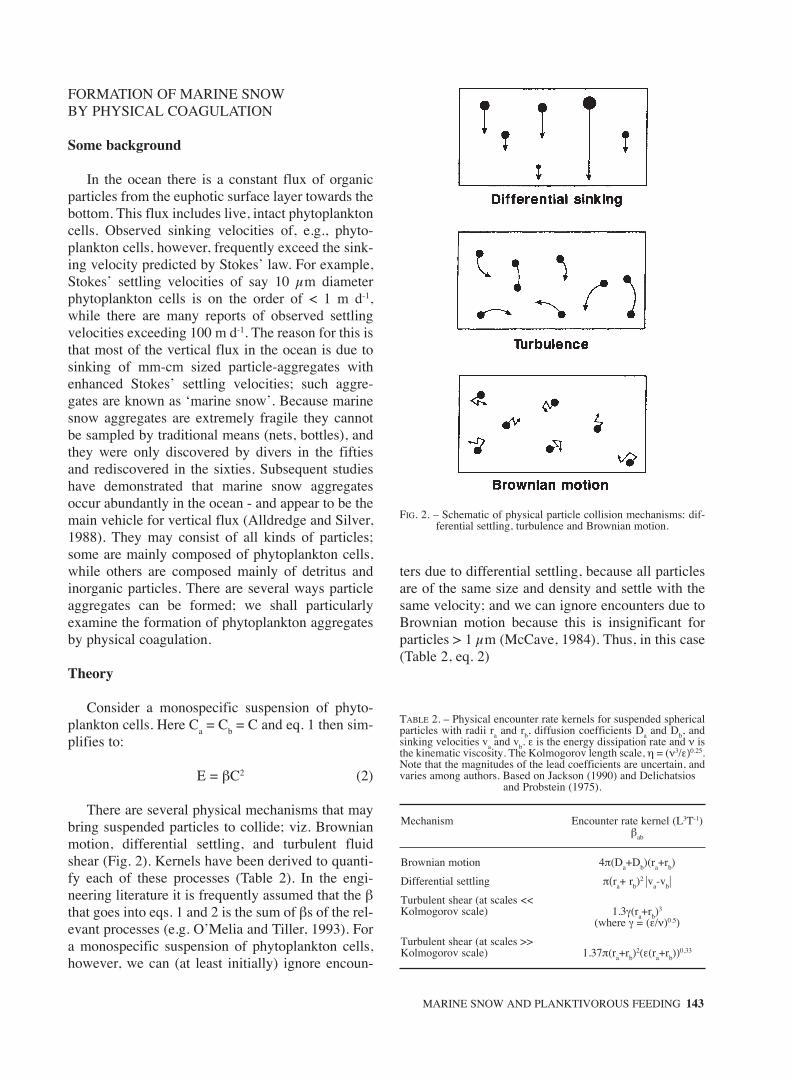
There are several physical mechanisms that maybring suspended particles to collide; viz. Brownianmotion, differential settling, and turbulent fluidshear (Fig. 2). Kernels have been derived to quanti-fy each of these processes (Table 2). In the engi-neering literature it is frequently assumed that the βthat goes into eqs. 1 and 2 is the sum of βs of the rel-evant processes (e.g. O’Melia and Tiller, 1993). Fora monospecific suspension of phytoplankton cells,however, we can (at least initially) ignore encoun-

ters due to differential settling, because all particlesare of the same size and density and settle with thesame velocity; and we can ignore encounters due toBrownian motion because this is insignificant forparticles > 1 µm (McCave, 1984). Thus, in this case(Table 2, eq. 2)

MARINE SNOW AND PLANKTIVOROUS FEEDING 143

FIG. 2. – Schematic of physical particle collision mechanisms: dif-ferential settling, turbulence and Brownian motion.

TABLE 2. – Physical encounter rate kernels for suspended sphericalparticles with radii ra and rb, diffusion coefficients Da and Db, andsinking velocities va and vb. ε is the energy dissipation rate and ν isthe kinematic viscosity. The Kolmogorov length scale, η = (ν3/ε)0.25.Note that the magnitudes of the lead coefficients are uncertain, andvaries among authors. Based on Jackson (1990) and Delichatsios

and Probstein (1975).

Mechanism Encounter rate kernel (L3T-1)βab

Brownian motion 4π(Da+Db)(ra+rb)

Differential settling π(ra+ rb)2 |va-vb|

Turbulent shear (at scales << Kolmogorov scale) 1.3γ(ra+rb)

3

(where γ = (ε/ν)0.5)

Turbulent shear (at scales >>Kolmogorov scale) 1.37π(ra+rb)

2(ε(ra+rb))0.33

E = 1.3γ(r1+r1)3C2 = 10.4γr1

3C2 (3)

Particles (or phytoplankton cells) that collidemay adhere upon collision provided they are‘sticky’. Assume that the probability of adhesionupon collision is given by the stickiness coefficientα. The concentration of single (unaggregated) cells(C1) suspended in a turbulent shear field will thendecline due to aggregation according to:

dC1/dt = -αE = -10.4αγr13C1

2 (4)

As coagulation proceeds aggregates consisting of2, 3, 4,... cells begin to form, and collisions betweensingle cells and small aggregates, and betweenaggregates of various sizes will occur. The book-keeping of all possible collisions can be accom-plished by infinitely many coupled differential equa-tions of the same principal form as equation (3).These are not easily managed (however, see Jacksonand Lochman 1992) but it can be shown that if oneconsiders only the initial process, a good approxi-mation is (Kiørboe et al., 1990):

Ct = C0e-α(7.8φγ/π)t (5)

where C0 is the initial concentration of cells, Ct is thetotal concentration of particles (single cells + aggre-gates consisting of 2, 3, 4,... cells) at time t, and φ isthe volume-concentration of cells (=4/3 πr1

3C0). Itcan likewise be shown that the average solid volumeof particles (including aggregates) will increaseaccording to:

Vt = V0eα(7.8φγ/π)t (6)

where V0 and Vt are the average volume of particlesat time 0 and t, respectively. Thus, theory predictsthat initially particle concentration will declineexponentially and average particle volume willincrease exponentially due to coagulation. Thisgrowth in particle size due to aggregation will leadto enhanced Stokes’ settling velocities and, hence, toincreased vertical flux of phytoplankton.

While these considerations present the basicideas of aggregate formation by physical coagula-tion and describe some of the fundamental proper-ties, the above simple equations do not contain allthe complexity of the real world. As aggregates ofvarious sizes are formed differential settling as acollision mechanism becomes important, as doesloss of particles from the system due to settling (e.g.

144 T. KIØRBOE

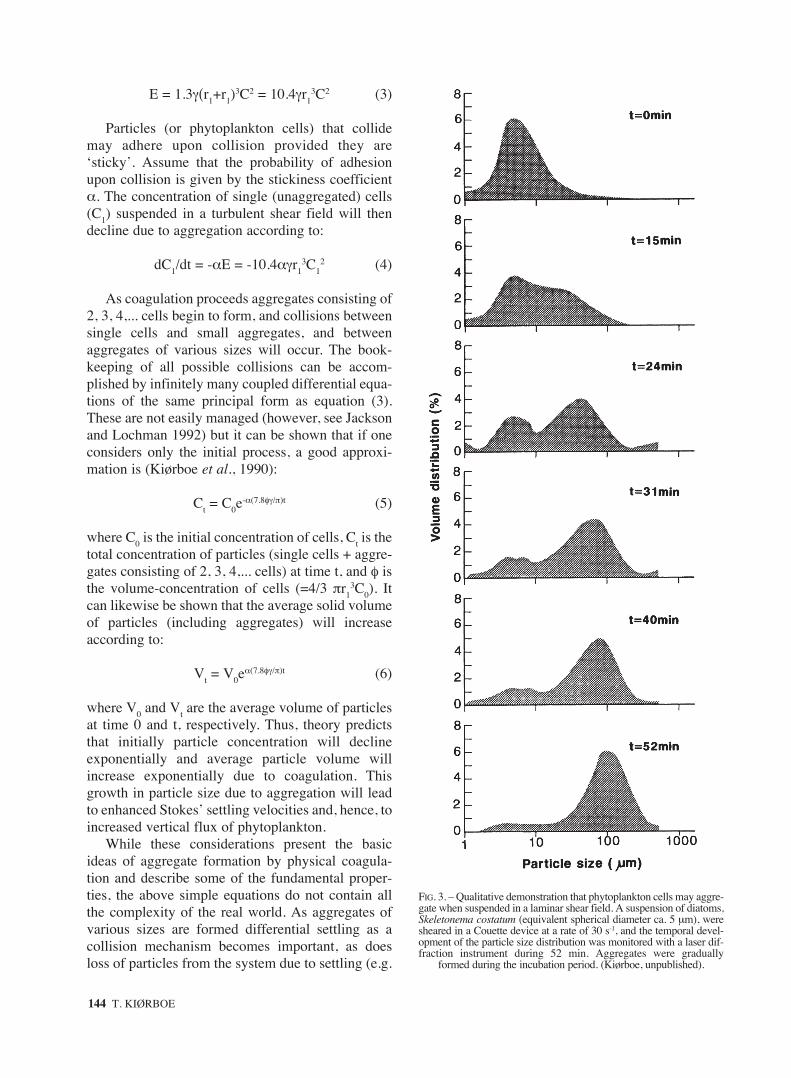
FIG. 3. – Qualitative demonstration that phytoplankton cells may aggre-gate when suspended in a laminar shear field. A suspension of diatoms,Skeletonema costatum (equivalent spherical diameter ca. 5 µm), weresheared in a Couette device at a rate of 30 s-1, and the temporal devel-opment of the particle size distribution was monitored with a laser dif-fraction instrument during 52 min. Aggregates were gradually

formed during the incubation period. (Kiørboe, unpublished).

Jackson, 1990; Jackson and Lochmann, 1992). Afurther complication is that collisions betweenunlike sized particles are restricted by hydrodynam-ics (e.g. Hill, 1992; Stolzenbach and Elimelech,1994). Finally, aggregates are fractal objects (e.g. Liand Logan, 1995); i.e., they are porous, and theirencased volume is larger than their solid volume,which, of course, has implications for their collisionrate with other particles and their further aggrega-tion. A treatment of these topics is beyond the scopeof this chapter (and the capability of the presentauthor); interested readers are referred to the abovequoted papers and references therein.

Evidence

Laboratory observations

While aggregate formation by physical coagula-tion has been demonstrated in many systems, e.g.,for particles in sewage treatment plants, the questionremains whether phytoplankton cells are sticky andcan aggregate as predicted by coagulation theory.Figs. 3 and 4 are qualitative and quantitative demon-strations, respectively, that this is in fact the case inlaboratory experiments. Phytoplankton cells(diatoms) were suspended in a shear field generatedin either a Couette device or by an oscillating grid.[A Couette device consists of two cylinders, eitheror both of them rotating, thus generating welldefined laminar shear in the annular gap between

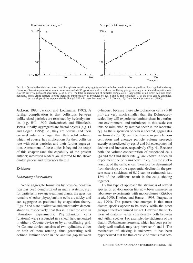
cylinders; because these phytoplankton cells (5-10µm) are very much smaller than the Kolmogorovscale, they will experience laminar shear in a turbu-lent environment, and turbulence at this scale canthus be mimicked by laminar shear in the laborato-ry]. As the suspension of cells is sheared, aggregatesare formed (Fig. 3), and the change in particle con-centration and average particle volume proceedsexactly as predicted by eqs. 5 and 6, i.e., exponentialdecline and increase, respectively (Fig. 4). Becauseboth the volume-concentration of suspended cells(φ) and the fluid shear rate (γ) are known in such anexperiment, the only unknown in eq. 5 is the sticki-ness, α, of the cells; α can therefore be determinedfrom the slope of the exponential decline. In the pre-sent case a stickiness of 0.12 can be estimated; i.e.,12% of the collisions result in the cells stickingtogether.

By this type of approach the stickiness of severalspecies of phytoplankton has now been measured inlaboratory experiments with monocultures (Kiørboeet al., 1990; Kiørboe and Hansen, 1993; Drapeau etal., 1994). The pattern that emerges is that mostdiatom species appear to be sticky while the othergroups hitherto examined are not. However, the stick-iness of diatoms varies considerably both betweenand within species. For example, the stickiness of thediatom Skeletonema costatum, which has been partic-ularly well studied, may vary between 0 and 1. Themechanism of sticking is unknown; it has beenhypothesized that the thin capsule of mucus that cov-

MARINE SNOW AND PLANKTIVOROUS FEEDING 145

FIG. 4. – Quantitative demonstration that phytoplankton cells may aggregate in a turbulent environment as predicted by coagulation theory.Diatoms, Phaeodactylum tricornutum, were suspended (33 ppm) in a beaker with an oscillating grid generating a turbulent dissipation rate,ε, of 25 cm2s-3 (equivalent shear rate, γ, of 50 s-1). The total concentration of particles (single cells + aggregates of all sizes) declines expo-nentially, and average particle volume increases exponentially, as predicted by eqs. 5 and 6. The stickiness, α, of the cells can be estimated

from the slope of the exponential decline (-0.029 min-1) (or increase) as 0.12 (from eq. 5). Data from Kiørboe et al. (1990).

ers many diatoms may act as a biological glue (e.g.Kiørboe and Hansen, 1993). This is supported by theobservation that bacterial exoenzymes, which digestmucus, may inhibit aggregation (Smith et al., 1995),and consistent with the observation in Skeletonemacostatum and other diatoms, that stickiness declinesas cultures age and the cells become overgrown withbacteria (Kiørboe et al., 1990; Dam and Drapeau,1995). Other diatoms may aggregate when sheared,even though their cell surface is not by itself sticky,e.g. Chaetoceros affinis. This diatom excretes organ-ic material that form 1-100 µm sized sticky mucusparticles; these particles may collide with cells and,thus, make them sticky (Kiørboe and Hansen, 1993;Passow et al., 1994).

Mesocosm and field observations

While there are several observations of phyto-plankton aggregates and aggregation in the ocean(e.g. Alldredge and Gotschalk, 1989; Riebesell,1991b; Tiselius and Kuylenstierna, 1996) there areonly very few field studies that have attempted toquantitatively compare observed aggregate forma-tion in the sea with predictions based on coagulationtheory.

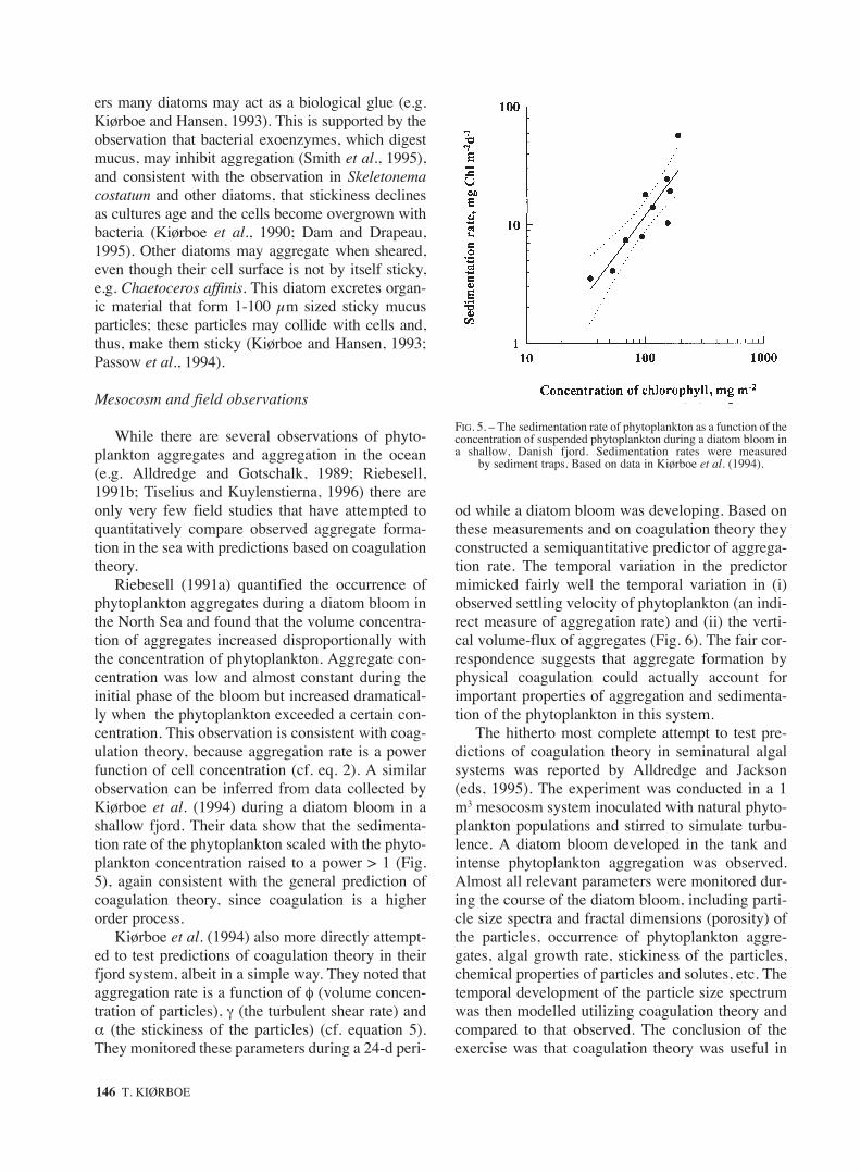
Riebesell (1991a) quantified the occurrence ofphytoplankton aggregates during a diatom bloom inthe North Sea and found that the volume concentra-tion of aggregates increased disproportionally withthe concentration of phytoplankton. Aggregate con-centration was low and almost constant during theinitial phase of the bloom but increased dramatical-ly when the phytoplankton exceeded a certain con-centration. This observation is consistent with coag-ulation theory, because aggregation rate is a powerfunction of cell concentration (cf. eq. 2). A similarobservation can be inferred from data collected byKiørboe et al. (1994) during a diatom bloom in ashallow fjord. Their data show that the sedimenta-tion rate of the phytoplankton scaled with the phyto-plankton concentration raised to a power > 1 (Fig.5), again consistent with the general prediction ofcoagulation theory, since coagulation is a higherorder process.

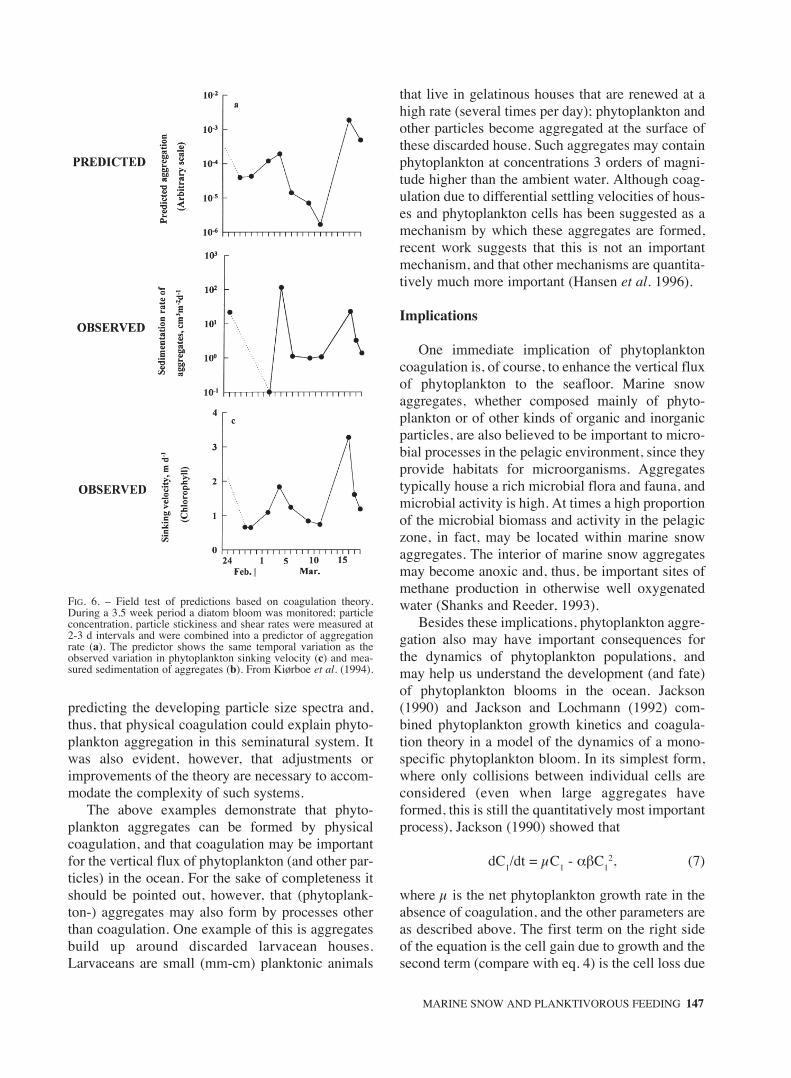
Kiørboe et al. (1994) also more directly attempt-ed to test predictions of coagulation theory in theirfjord system, albeit in a simple way. They noted thataggregation rate is a function of φ (volume concen-tration of particles), γ (the turbulent shear rate) andα (the stickiness of the particles) (cf. equation 5).They monitored these parameters during a 24-d peri-

od while a diatom bloom was developing. Based onthese measurements and on coagulation theory theyconstructed a semiquantitative predictor of aggrega-tion rate. The temporal variation in the predictormimicked fairly well the temporal variation in (i)observed settling velocity of phytoplankton (an indi-rect measure of aggregation rate) and (ii) the verti-cal volume-flux of aggregates (Fig. 6). The fair cor-respondence suggests that aggregate formation byphysical coagulation could actually account forimportant properties of aggregation and sedimenta-tion of the phytoplankton in this system.

The hitherto most complete attempt to test pre-dictions of coagulation theory in seminatural algalsystems was reported by Alldredge and Jackson(eds, 1995). The experiment was conducted in a 1m3 mesocosm system inoculated with natural phyto-plankton populations and stirred to simulate turbu-lence. A diatom bloom developed in the tank andintense phytoplankton aggregation was observed.Almost all relevant parameters were monitored dur-ing the course of the diatom bloom, including parti-cle size spectra and fractal dimensions (porosity) ofthe particles, occurrence of phytoplankton aggre-gates, algal growth rate, stickiness of the particles,chemical properties of particles and solutes, etc. Thetemporal development of the particle size spectrumwas then modelled utilizing coagulation theory andcompared to that observed. The conclusion of theexercise was that coagulation theory was useful in

146 T. KIØRBOE

FIG. 5. – The sedimentation rate of phytoplankton as a function of theconcentration of suspended phytoplankton during a diatom bloom ina shallow, Danish fjord. Sedimentation rates were measured

by sediment traps. Based on data in Kiørboe et al. (1994).

predicting the developing particle size spectra and,thus, that physical coagulation could explain phyto-plankton aggregation in this seminatural system. Itwas also evident, however, that adjustments orimprovements of the theory are necessary to accom-modate the complexity of such systems.

The above examples demonstrate that phyto-plankton aggregates can be formed by physicalcoagulation, and that coagulation may be importantfor the vertical flux of phytoplankton (and other par-ticles) in the ocean. For the sake of completeness itshould be pointed out, however, that (phytoplank-ton-) aggregates may also form by processes otherthan coagulation. One example of this is aggregatesbuild up around discarded larvacean houses.Larvaceans are small (mm-cm) planktonic animals

that live in gelatinous houses that are renewed at ahigh rate (several times per day); phytoplankton andother particles become aggregated at the surface ofthese discarded house. Such aggregates may containphytoplankton at concentrations 3 orders of magni-tude higher than the ambient water. Although coag-ulation due to differential settling velocities of hous-es and phytoplankton cells has been suggested as amechanism by which these aggregates are formed,recent work suggests that this is not an importantmechanism, and that other mechanisms are quantita-tively much more important (Hansen et al. 1996).

Implications

One immediate implication of phytoplanktoncoagulation is, of course, to enhance the vertical fluxof phytoplankton to the seafloor. Marine snowaggregates, whether composed mainly of phyto-plankton or of other kinds of organic and inorganicparticles, are also believed to be important to micro-bial processes in the pelagic environment, since theyprovide habitats for microorganisms. Aggregatestypically house a rich microbial flora and fauna, andmicrobial activity is high. At times a high proportionof the microbial biomass and activity in the pelagiczone, in fact, may be located within marine snowaggregates. The interior of marine snow aggregatesmay become anoxic and, thus, be important sites ofmethane production in otherwise well oxygenatedwater (Shanks and Reeder, 1993).

Besides these implications, phytoplankton aggre-gation also may have important consequences forthe dynamics of phytoplankton populations, andmay help us understand the development (and fate)of phytoplankton blooms in the ocean. Jackson(1990) and Jackson and Lochmann (1992) com-bined phytoplankton growth kinetics and coagula-tion theory in a model of the dynamics of a mono-specific phytoplankton bloom. In its simplest form,where only collisions between individual cells areconsidered (even when large aggregates haveformed, this is still the quantitatively most importantprocess), Jackson (1990) showed that

dC1/dt = µC1 - αβC12, (7)

where µ is the net phytoplankton growth rate in theabsence of coagulation, and the other parameters areas described above. The first term on the right sideof the equation is the cell gain due to growth and thesecond term (compare with eq. 4) is the cell loss due

MARINE SNOW AND PLANKTIVOROUS FEEDING 147

FIG. 6. – Field test of predictions based on coagulation theory.During a 3.5 week period a diatom bloom was monitored; particleconcentration, particle stickiness and shear rates were measured at2-3 d intervals and were combined into a predictor of aggregationrate (a). The predictor shows the same temporal variation as theobserved variation in phytoplankton sinking velocity (c) and mea-sured sedimentation of aggregates (b). From Kiørboe et al. (1994).

to coagulation (and subsequent sedimentation). Thismodel predicts a sigmoid population growth curvefor the phytoplankton, even when light and nutrientsupply to the phytoplankton is constant, and thegrowth rate, therefore, constant. Kiørboe et al.(1994) examined exactly such a situation, anddemonstrated that the populations of 5 species ofdiatoms showed sigmoid growth. Because the cellgain increases linearly with cell concentration whilethe cell loss scales with the concentration squared,coagulation becomes relatively more important asthe population increases. There will be a cell con-centration (CCr) at which growth is balanced bycoagulation, and cell concentration is constant.Putting dC1/dt = 0 and inserting the expression for β(Table 2) in eq. 7 yields

CCr = 0.096µ(αγr3)-1 (8)

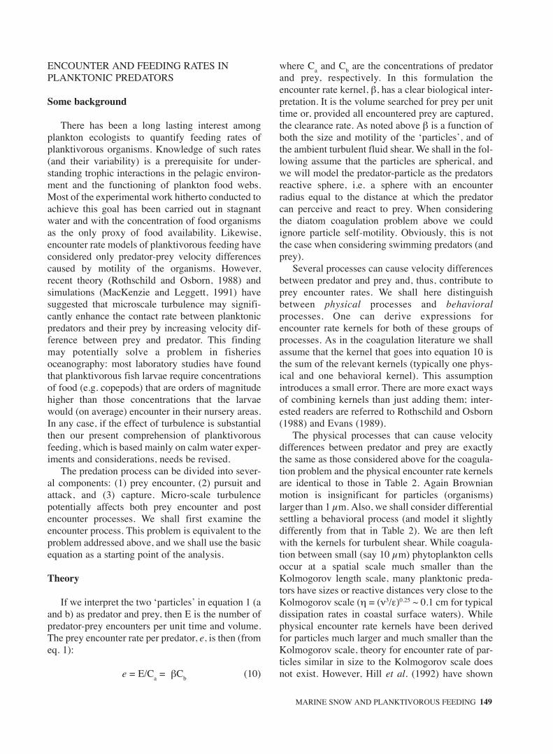
This simple model actually predicts fairly accu-rately the diatom equilibrium concentrations foundby Kiørboe et al. (1994) (Fig. 7). This approach ignores the fact that species may

interact; i.e., that interspecific aggregation mayoccur. Kiørboe et al. (1994) expanded Jackson’ssimple model to take interspecific aggregation intoaccount. Due to coagulation the concentration of thei’th species will change according to:

dCi/dt = µiCi -Ci∑αijCjχijβij (9)

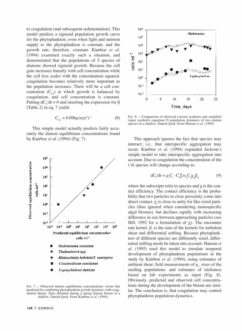
where the subscripts refer to species and χ is the con-tact efficiency. The contact efficiency is the proba-bility that two particles in close proximity come intodirect contact. χ is close to unity for like-sized parti-cles (thus ignored when considering monospecificalgal blooms), but declines rapidly with increasingdifference in size between approaching particles (seeHill, 1992 for a formulation of χ). The encounterrate kernel, β, is the sum of the kernels for turbulentshear and differential settling. Because phytoplank-ters of different species are differently sized, differ-ential settling needs be taken into account. Hansen etal. (1995) used this model to simulate temporaldevelopment of phytoplankton populations in thestudy by Kiørboe et al. (1994), using estimates ofambient shear, field measurements of µi, sizes of theseeding populations, and estimates of stickinessbased on lab experiments as input (Fig. 8).Obviously, predicted and observed cell concentra-tions during the development of the bloom are simi-lar. The conclusion is, that coagulation may controlphytoplankton population dynamics.

148 T. KIØRBOE

FIG. 7. – Observed diatom equilibrium concentrations versus thatpredicted by combining phytoplankton growth dynamics with coag-ulation theory. Data obtained during a spring diatom bloom in a

shallow, Danish fjord. From Kiørboe et al. (1994).

FIG. 8. – Comparison of observed (closed symbols) and modelled(open symbols) (equation 9) population dynamics of two diatomspecies in a shallow, Danish fjord. From Hansen et al. (1995)

ENCOUNTER AND FEEDING RATES INPLANKTONIC PREDATORS

Some background

There has been a long lasting interest amongplankton ecologists to quantify feeding rates ofplanktivorous organisms. Knowledge of such rates(and their variability) is a prerequisite for under-standing trophic interactions in the pelagic environ-ment and the functioning of plankton food webs.Most of the experimental work hitherto conducted toachieve this goal has been carried out in stagnantwater and with the concentration of food organismsas the only proxy of food availability. Likewise,encounter rate models of planktivorous feeding haveconsidered only predator-prey velocity differencescaused by motility of the organisms. However,recent theory (Rothschild and Osborn, 1988) andsimulations (MacKenzie and Leggett, 1991) havesuggested that microscale turbulence may signifi-cantly enhance the contact rate between planktonicpredators and their prey by increasing velocity dif-ference between prey and predator. This findingmay potentially solve a problem in fisheriesoceanography: most laboratory studies have foundthat planktivorous fish larvae require concentrationsof food (e.g. copepods) that are orders of magnitudehigher than those concentrations that the larvaewould (on average) encounter in their nursery areas.In any case, if the effect of turbulence is substantialthen our present comprehension of planktivorousfeeding, which is based mainly on calm water exper-iments and considerations, needs be revised.

The predation process can be divided into sever-al components: (1) prey encounter, (2) pursuit andattack, and (3) capture. Micro-scale turbulencepotentially affects both prey encounter and postencounter processes. We shall first examine theencounter process. This problem is equivalent to theproblem addressed above, and we shall use the basicequation as a starting point of the analysis.

Theory

If we interpret the two ‘particles’ in equation 1 (aand b) as predator and prey, then E is the number ofpredator-prey encounters per unit time and volume.The prey encounter rate per predator, e, is then (fromeq. 1):

e = E/Ca = βCb (10)

where Ca and Cb are the concentrations of predatorand prey, respectively. In this formulation theencounter rate kernel, β, has a clear biological inter-pretation. It is the volume searched for prey per unittime or, provided all encountered prey are captured,the clearance rate. As noted above β is a function ofboth the size and motility of the ‘particles’, and ofthe ambient turbulent fluid shear. We shall in the fol-lowing assume that the particles are spherical, andwe will model the predator-particle as the predatorsreactive sphere, i.e. a sphere with an encounterradius equal to the distance at which the predatorcan perceive and react to prey. When consideringthe diatom coagulation problem above we couldignore particle self-motility. Obviously, this is notthe case when considering swimming predators (andprey).

Several processes can cause velocity differencesbetween predator and prey and, thus, contribute toprey encounter rates. We shall here distinguishbetween physical processes and behavioralprocesses. One can derive expressions forencounter rate kernels for both of these groups ofprocesses. As in the coagulation literature we shallassume that the kernel that goes into equation 10 isthe sum of the relevant kernels (typically one phys-ical and one behavioral kernel). This assumptionintroduces a small error. There are more exact waysof combining kernels than just adding them; inter-ested readers are referred to Rothschild and Osborn(1988) and Evans (1989).

The physical processes that can cause velocitydifferences between predator and prey are exactlythe same as those considered above for the coagula-tion problem and the physical encounter rate kernelsare identical to those in Table 2. Again Brownianmotion is insignificant for particles (organisms)larger than 1 µm. Also, we shall consider differentialsettling a behavioral process (and model it slightlydifferently from that in Table 2). We are then leftwith the kernels for turbulent shear. While coagula-tion between small (say 10 µm) phytoplankton cellsoccur at a spatial scale much smaller than theKolmogorov length scale, many planktonic preda-tors have sizes or reactive distances very close to theKolmogorov scale (η = (ν3/ε)0.25 ~ 0.1 cm for typicaldissipation rates in coastal surface waters). Whilephysical encounter rate kernels have been derivedfor particles much larger and much smaller than theKolmogorov scale, theory for encounter rate of par-ticles similar in size to the Kolmogorov scale doesnot exist. However, Hill et al. (1992) have shown

MARINE SNOW AND PLANKTIVOROUS FEEDING 149

experimentally that supra-Kolmogorov scale theoryapplies at, or even somewhat below, theKolmogorov scale. While this appears to be contro-versial and not generally accepted, we shall makethis assumption in the following.

There has been some confusion in the literatureas to the appropriate scale to be used when calculat-ing the velocity difference due to turbulence. Herewe assume that the predators reaction distance (+ theradius of the prey) is the correct scale (cf. Table 2);see Kiørboe and MacKenzie (1995) for a discussionof the issue.

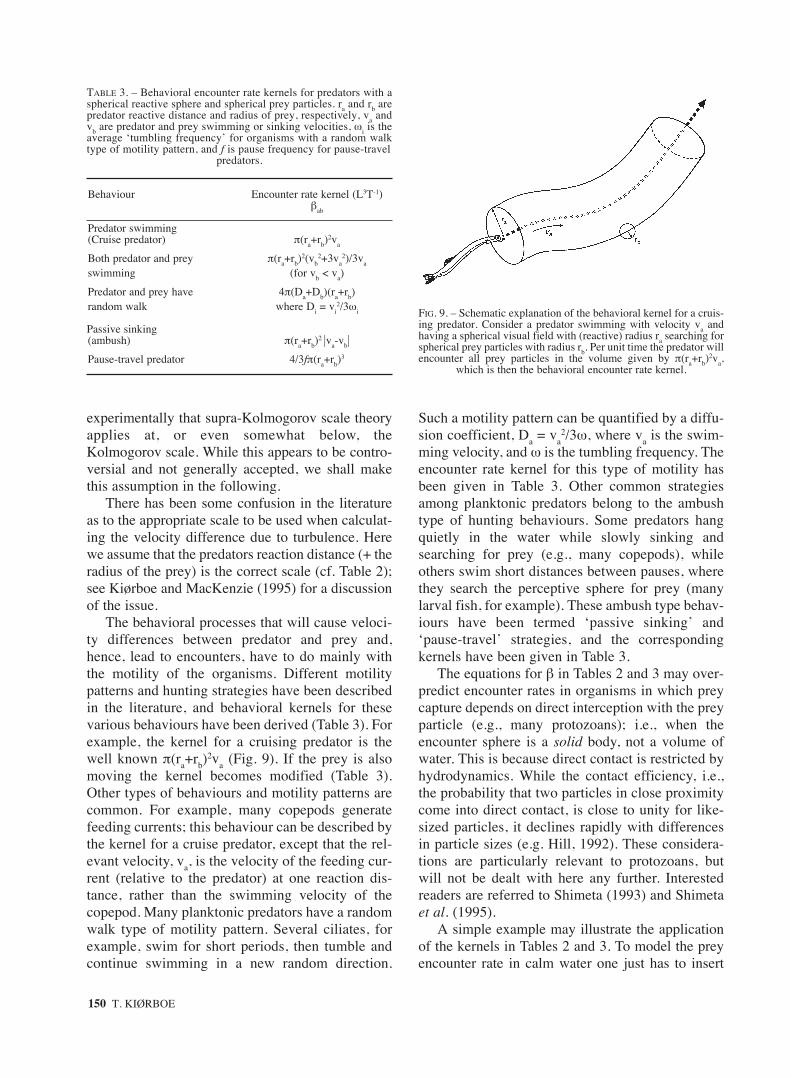
The behavioral processes that will cause veloci-ty differences between predator and prey and,hence, lead to encounters, have to do mainly withthe motility of the organisms. Different motilitypatterns and hunting strategies have been describedin the literature, and behavioral kernels for thesevarious behaviours have been derived (Table 3). Forexample, the kernel for a cruising predator is thewell known π(ra+rb)

2va (Fig. 9). If the prey is alsomoving the kernel becomes modified (Table 3).Other types of behaviours and motility patterns arecommon. For example, many copepods generatefeeding currents; this behaviour can be described bythe kernel for a cruise predator, except that the rel-evant velocity, va, is the velocity of the feeding cur-rent (relative to the predator) at one reaction dis-tance, rather than the swimming velocity of thecopepod. Many planktonic predators have a randomwalk type of motility pattern. Several ciliates, forexample, swim for short periods, then tumble andcontinue swimming in a new random direction.

Such a motility pattern can be quantified by a diffu-sion coefficient, Da = va

2/3ω, where va is the swim-ming velocity, and ω is the tumbling frequency. Theencounter rate kernel for this type of motility hasbeen given in Table 3. Other common strategiesamong planktonic predators belong to the ambushtype of hunting behaviours. Some predators hangquietly in the water while slowly sinking andsearching for prey (e.g., many copepods), whileothers swim short distances between pauses, wherethey search the perceptive sphere for prey (manylarval fish, for example). These ambush type behav-iours have been termed ‘passive sinking’ and‘pause-travel’ strategies, and the correspondingkernels have been given in Table 3.

The equations for β in Tables 2 and 3 may over-predict encounter rates in organisms in which preycapture depends on direct interception with the preyparticle (e.g., many protozoans); i.e., when theencounter sphere is a solid body, not a volume ofwater. This is because direct contact is restricted byhydrodynamics. While the contact efficiency, i.e.,the probability that two particles in close proximitycome into direct contact, is close to unity for like-sized particles, it declines rapidly with differencesin particle sizes (e.g. Hill, 1992). These considera-tions are particularly relevant to protozoans, butwill not be dealt with here any further. Interestedreaders are referred to Shimeta (1993) and Shimetaet al. (1995).

A simple example may illustrate the applicationof the kernels in Tables 2 and 3. To model the preyencounter rate in calm water one just has to insert

150 T. KIØRBOE

TABLE 3. – Behavioral encounter rate kernels for predators with aspherical reactive sphere and spherical prey particles. ra and rb arepredator reactive distance and radius of prey, respectively, va andvb are predator and prey swimming or sinking velocities, ωi is theaverage ‘tumbling frequency’ for organisms with a random walktype of motility pattern, and f is pause frequency for pause-travel

predators.

Behaviour Encounter rate kernel (L3T-1)βab

Predator swimming (Cruise predator) π(ra+rb)

2va

Both predator and prey π(ra+rb)2(vb

2+3va2)/3va

swimming (for vb < va)

Predator and prey have 4π(Da+Db)(ra+rb)random walk where Di = vi

2/3ωi

Passive sinking (ambush) π(ra+rb)

2 |va-vb|

Pause-travel predator 4/3fπ(ra+rb)3

FIG. 9. – Schematic explanation of the behavioral kernel for a cruis-ing predator. Consider a predator swimming with velocity va andhaving a spherical visual field with (reactive) radius ra searching forspherical prey particles with radius rb. Per unit time the predator willencounter all prey particles in the volume given by π(ra+rb)

2va,which is then the behavioral encounter rate kernel.

the relevant behavioral kernel in eq. 10. To modelprey encounter in a turbulent environment, β in eq.10 is assumed to be the sum of the relevant behav-ioral and physical kernels, β= βbehaviour+βturbulence. Forexample, assume that the cruising predator in Fig. 9is a herring larva with a reaction distance (ra) of 1.5cm and a swimming velocity (va) of 1 cm s-1. If weignore the motility and size of the prey (copepodnauplii), because they are both very small, then incalm water β = βbehaviour = πx1.52x1 = 7.1 cm3 s-1 (~25 l h-1). Assume now that the larva experiences aturbulent environment characterized by a dissipationrate ε = 10-2 cm2 s-3 (typical for coastal surfacewaters). Then, β = βbehaviour+βturbulence = 7.1 +1.37x1.52x(10-2x1.5)0.33 = 7.9 cm3 s-1 (~ 28 l h-1).Thus, in this imaginary example, turbulence of thismagnitude will increase the volume searched forprey by only 3/25 = 12%. In a similar manner ker-nels for turbulence and behaviour (Tables 2 and 3)can be combined to examine the effect of turbulenceon prey encounter rates for predators with variousbehaviours and behavioral parameters, and at vari-ous intensities of turbulence.

In the above example it was assumed that thebehaviour of the predator was unaffected by turbu-lence. This is not necessarily the case. Thus, thereare several examples that predators change swim-ming speeds, reactive distances and/or time allocat-ed to searching for food as a function of turbulence

(e.g., Costello et al., 1990; Saiz, 1994). If thechanges in the relevant behavioral parameters (i.e.,in the above example: time spent searching for food,swimming velocity and reactive distance) can bequantified, it is a simple task to account for it in themodel.

Evidence

Observational evidence is accumulating, thatsmall-scale turbulence in fact enhances preyencounter and feeding rates in planktivorous preda-tors. Thus, positive effects of turbulence have beendemonstrated in both laboratory and field experi-ments for protozoa (Shimeta et al., 1995; Peters andGross, 1994), copepods (Saiz et al., 1992; Marraséet al., 1990; Saiz and Kiørboe, 1995; Kiørboe, 1993)and fish larvae (Sundby and Fossum 1990; Sundbyet al., 1994, MacKenzie and Kiørboe, 1995).However, only few experiments have been designedto quantitatively test the predictions of the modelsdescribed above.

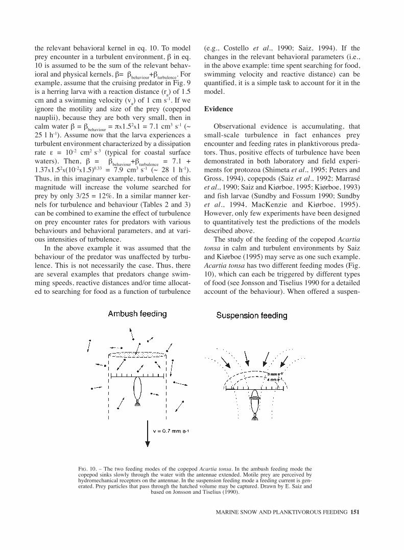
The study of the feeding of the copepod Acartiatonsa in calm and turbulent environments by Saizand Kiørboe (1995) may serve as one such example.Acartia tonsa has two different feeding modes (Fig.10), which can each be triggered by different typesof food (see Jonsson and Tiselius 1990 for a detailedaccount of the behaviour). When offered a suspen-

MARINE SNOW AND PLANKTIVOROUS FEEDING 151

FIG. 10. – The two feeding modes of the copepod Acartia tonsa. In the ambush feeding mode thecopepod sinks slowly through the water with the antennae extended. Motile prey are perceived byhydromechanical receptors on the antennae. In the suspension feeding mode a feeding current is gen-erated. Prey particles that pass through the hatched volume may be captured. Drawn by E. Saiz and

based on Jonsson and Tiselius (1990).

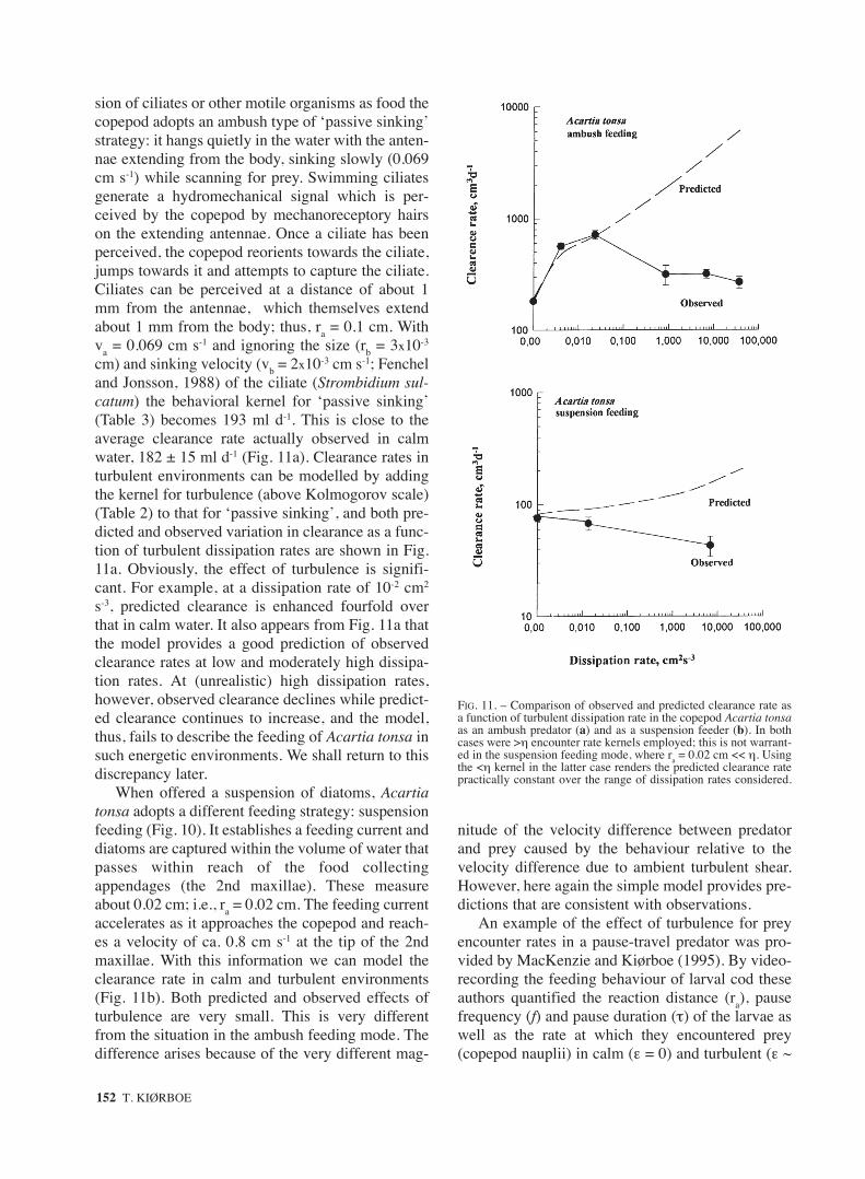
sion of ciliates or other motile organisms as food thecopepod adopts an ambush type of ‘passive sinking’strategy: it hangs quietly in the water with the anten-nae extending from the body, sinking slowly (0.069cm s-1) while scanning for prey. Swimming ciliatesgenerate a hydromechanical signal which is per-ceived by the copepod by mechanoreceptory hairson the extending antennae. Once a ciliate has beenperceived, the copepod reorients towards the ciliate,jumps towards it and attempts to capture the ciliate.Ciliates can be perceived at a distance of about 1mm from the antennae, which themselves extendabout 1 mm from the body; thus, ra = 0.1 cm. Withva = 0.069 cm s-1 and ignoring the size (rb = 3x10-3

cm) and sinking velocity (vb = 2x10-3 cm s-1; Fencheland Jonsson, 1988) of the ciliate (Strombidium sul-catum) the behavioral kernel for ‘passive sinking’(Table 3) becomes 193 ml d-1. This is close to theaverage clearance rate actually observed in calmwater, 182 ± 15 ml d-1 (Fig. 11a). Clearance rates inturbulent environments can be modelled by addingthe kernel for turbulence (above Kolmogorov scale)(Table 2) to that for ‘passive sinking’, and both pre-dicted and observed variation in clearance as a func-tion of turbulent dissipation rates are shown in Fig.11a. Obviously, the effect of turbulence is signifi-cant. For example, at a dissipation rate of 10-2 cm2

s-3, predicted clearance is enhanced fourfold overthat in calm water. It also appears from Fig. 11a thatthe model provides a good prediction of observedclearance rates at low and moderately high dissipa-tion rates. At (unrealistic) high dissipation rates,however, observed clearance declines while predict-ed clearance continues to increase, and the model,thus, fails to describe the feeding of Acartia tonsa insuch energetic environments. We shall return to thisdiscrepancy later.

When offered a suspension of diatoms, Acartiatonsa adopts a different feeding strategy: suspensionfeeding (Fig. 10). It establishes a feeding current anddiatoms are captured within the volume of water thatpasses within reach of the food collectingappendages (the 2nd maxillae). These measureabout 0.02 cm; i.e., ra = 0.02 cm. The feeding currentaccelerates as it approaches the copepod and reach-es a velocity of ca. 0.8 cm s-1 at the tip of the 2ndmaxillae. With this information we can model theclearance rate in calm and turbulent environments(Fig. 11b). Both predicted and observed effects ofturbulence are very small. This is very differentfrom the situation in the ambush feeding mode. Thedifference arises because of the very different mag-

nitude of the velocity difference between predatorand prey caused by the behaviour relative to thevelocity difference due to ambient turbulent shear.However, here again the simple model provides pre-dictions that are consistent with observations.

An example of the effect of turbulence for preyencounter rates in a pause-travel predator was pro-vided by MacKenzie and Kiørboe (1995). By video-recording the feeding behaviour of larval cod theseauthors quantified the reaction distance (ra), pausefrequency (f) and pause duration (τ) of the larvae aswell as the rate at which they encountered prey(copepod nauplii) in calm (ε = 0) and turbulent (ε ~

152 T. KIØRBOE

FIG. 11. – Comparison of observed and predicted clearance rate asa function of turbulent dissipation rate in the copepod Acartia tonsaas an ambush predator (a) and as a suspension feeder (b). In bothcases were >η encounter rate kernels employed; this is not warrant-ed in the suspension feeding mode, where ra = 0.02 cm << η. Usingthe <η kernel in the latter case renders the predicted clearance ratepractically constant over the range of dissipation rates considered.

10-3 cm2s-3) environments. By combining the kernelsfor turbulence and pause-travel feeding they predict-ed that larvae in this size range (5.2-6.1 mm length)should increase their encounter rate with prey 2.2-3.2-fold; they observed a 2.2-4.7-fold increase. Inthis comparison observed changes in behavioralparameters (pause frequency and pause duration) inturbulent as compared to calm water were taken intoaccount. Thus, apparently the simple model wasable to predict the magnitude of the increase in preyencounter rate.

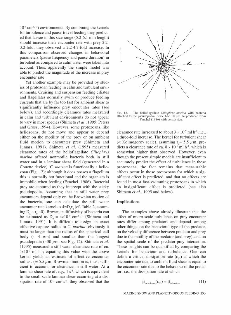
Yet another example may be provided by stud-ies of protozoan feeding in calm and turbulent envi-ronments. Cruising and suspension feeding ciliatesand flagellates normally swim or produce feedingcurrents that are by far too fast for ambient shear tosignificantly influence prey encounter rates (seebelow), and accordingly clearance rates measuredin calm and turbulent environments do not appearto vary in most species (Shimeta et al., 1995; Petersand Gross, 1994). However, some protozoans, likeheliozoans, do not move and appear to dependeither on the motility of the prey or on ambientfluid motion to encounter prey (Shimeta andJumars, 1991). Shimeta et al. (1995) measuredclearance rates of the helioflagellate Ciliophrysmarina offered nonmotile bacteria both in stillwater and in a laminar shear field (generated in aCouette device). C. marina is functionally a helio-zoan (Fig. 12); although it does posses a flagellumthis is normally not functional and the organism isimmobile when feeding (Fenchel, 1986). Bacterialprey are captured as they intercept with the stickypseudopodia. Assuming that in still water preyencounters depend only on the Brownian motion ofthe bacteria, one can calculate the still waterencounter rate kernel as 4πDbra (cf. Table 2, assum-ing Da ~ rb ~0). Brownian diffusivity of bacteria canbe estimated as Db = 4×10-9 cm2 s-1 (Shimeta andJumars, 1991). It is difficult to assign an exacteffective capture radius to C. marina; obviously itmust be larger than the radius of the spherical cellbody (~ 4 µm) and smaller than the longestpseudopodia (~30 µm; see Fig. 12). Shimeta et al.(1995) measured a still water clearance rate of ca.1x10-7 ml h-1; equating this value with the abovekernel yields an estimate of effective encounterradius, ra= 5.5 µm. Brownian motion is, thus, suffi-cient to account for clearance in still water. At alaminar shear rate of, e.g., 1 s-1, which is equivalentto the small-scale laminar shear occurring at a dis-sipation rate of 10-2 cm2 s-3, they observed that the

clearance rate increased to about 3 × 10-7 ml h-1, i.e.,a three-fold increase. The kernel for turbulent shear(< Kolmogorov scale), assuming ra= 5.5 µm, pre-dicts a clearance rate of ca. 8 × 10-6 ml h-1, which issomewhat higher than observed. However, eventhough the present simple models are insufficient toaccurately predict the effect of turbulence in theseprotozoans, the fact remains that measurableeffects occur in those protozoans for which a sig-nificant effect is predicted, and that no effects arefound in most fast-swimming protozoans in whichan insignificant effect is predicted (see alsoShimeta et al., 1995 and below).

Implications

The examples above already illustrate that theeffect of micro-scale turbulence on prey encounterrates differ among predators and depend, amongother things, on the behavioral type of the predator,on the velocity difference between predator and preydue to the motility of the predator (and prey), and onthe spatial scale of the predator-prey interaction.These insights can be quantified by comparing thekernels for behaviour and turbulence. One candefine a critical dissipation rate (εCr) at which theencounter rate due to ambient fluid shear is equal tothe encounter rate due to the behaviour of the preda-tor; i.e., the dissipation rate at which

βturbulence(εCr) = βbehaviour (11)

MARINE SNOW AND PLANKTIVOROUS FEEDING 153

FIG. 12. – The helioflagellate Ciliophrys marina with bacteriaattached to the pseudopodia. Scale bar: 10 µm. Reproduced from

Fenchel (1986) with permission.

Thus, at dissipation rates exceeding εCr, turbu-lence is more important than behaviour for preyencounter; and vice versa. In the foregoing we haveidentified two different kernels for turbulence, andwe have defined four different behavioral types andtheir associated kernels (Table 2 and 3). This yieldseight different combinations of behaviour and turbu-lence. For simplicity we shall in the followingignore the motility and size of the prey, becausethese are often (but not always) small compared tothe motility and behaviour of the predator. Let usfirst examine the random walk type of predatormotility pattern at scales > Kolmogorov scale.Inserting the relevant kernels form Tables 2 and 3into eq. 11 yields:

1.37πra2(εCrra)

0.33= 4πDara

which simplifies to

εCr = 24.9Da3ra

-4

and likewise for scales smaller than the Kolmogorovscale:

εCr = 93Da2ra

-4ν

where we recall that ν is the kinematic viscosity (~10-2 cm2s-1). In a similar fashion critical dissipationrates can be derived for the other behavioral types(Table 4). Note that the formula for the critical dis-sipation rate is the same for cruising predators, pas-sively sinking predators, and for predators that gen-erate a feeding current, but that the interpretation ofthe velocity (va) varies (swimming velocity, sinkingvelocity, and velocity of the feeding current at onereaction distance away from the predator, respec-

tively). Note also that the magnitude of the leadcoefficients in these expressions may vary (up toone order of magnitude) depending on the assumedmagnitude of the lead coefficients in the governing

154 T. KIØRBOE

TABLE 4. – Critical dissipation rates for predators with different for-aging strategies operating at scales above and below theKolmogorov length scale (η). The lead coefficients may vary (up toan order of magnitude) depending on the magnitude of the leadcoefficient in the governing equations, and on the way kernels havebeen combined. Here we have combined kernels as suggested by

Evans (1989). Parameters as in Tables 2 and 3.

Predator behaviour\Spatial scale ra>η ra<η

Cruise predatorpassive sinkingSuspension feeder 0.14va

3ra-1 1.7va

2ra-2ν

Random walk 25Da3ra

-4 93Da2ra

- 4ν

Pause-travel predator 0.33ra2τ-3 10τ-2ν

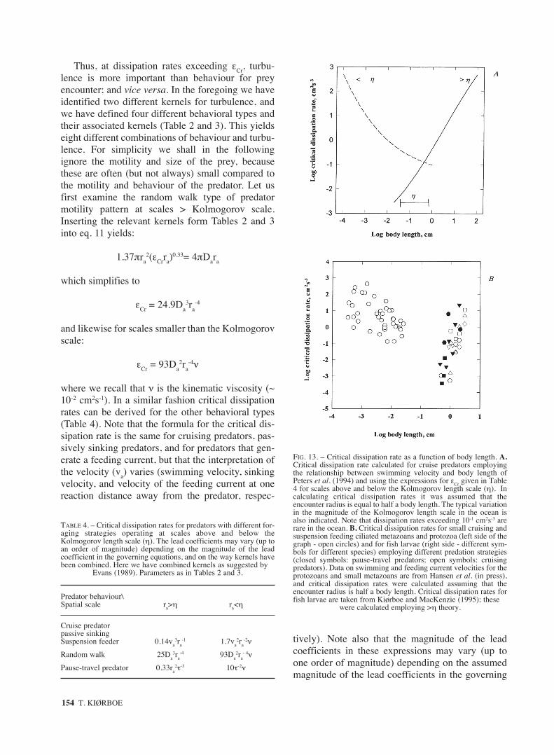
FIG. 13. – Critical dissipation rate as a function of body length. A.Critical dissipation rate calculated for cruise predators employingthe relationship between swimming velocity and body length ofPeters et al. (1994) and using the expressions for εCr given in Table4 for scales above and below the Kolmogorov length scale (η). Incalculating critical dissipation rates it was assumed that theencounter radius is equal to half a body length. The typical variationin the magnitude of the Kolmogorov length scale in the ocean isalso indicated. Note that dissipation rates exceeding 10-1 cm2s-3 arerare in the ocean. B. Critical dissipation rates for small cruising andsuspension feeding ciliated metazoans and protozoa (left side of thegraph - open circles) and for fish larvae (right side - different sym-bols for different species) employing different predation strategies(closed symbols: pause-travel predators; open symbols: cruisingpredators). Data on swimming and feeding current velocities for theprotozoans and small metazoans are from Hansen et al. (in press),and critical dissipation rates were calculated assuming that theencounter radius is half a body length. Critical dissipation rates forfish larvae are taken from Kiørboe and MacKenzie (1995); these

were calculated employing >η theory.

equations, on the way that kernels are combined,and on modifications of the kernels relevant todetails in the behaviour of specific organisms. Theform of the expressions, however, are invariant withthese variations in assumptions. In Table 4, kernelshave been combined in the way suggested by Evans(1989); see also Kiørboe and MacKenzie (1995).

The form of the equations for critical dissipationrate suggest that this is minimum at scales near theKolmogorov length scale (η), at least for cruisingpredators (Fig. 13a,b). In other words, turbulenceappears to be potentially most important for plank-tivorous predators with an encounter radius close toη. To see this, consider first predators smaller thanη; for these, εCr scales with the ratio of swimmingvelocity to encounter radius squared, (va/ra)

2 (Table4). Swimming or feeding current velocities in fla-gellates, ciliates and other small ciliated cruisingand suspension feeding predators (e.g. rotifers)depends only weakly on size (Peters et al., 1994.)and appear to scale with size raised to exponentsconsiderably less than one (e.g., 0.24, Sommer,1988; 0.6, Hansen et al., in press). For these preda-tors the encounter radius is typically simply theradius of the (assumed spherical) body and it, thus,follows that (va/ra)

2 and, hence, εCr decrease withsize. For predators with encounter radius > η thecritical dissipation rate scale with va

3/ra (Table 4).For such predators (e.g. fish larvae) both swimmingvelocity and reactive distance appear to increasealmost proportionally to body length (e.g. Blaxter,1986; Miller et al., 1988). Thus, va

3/ra and εCrincreases with size and it follows that εCr is mini-mum for predators with encounter radius near η.

Fig. 13a,b illustrates this relation between εCr andorganism size. Peters et al. (1994) compiled litera-ture data on swimming velocities in aquatic organ-isms ranging from bacteria to whales, and by regres-sion defined a relation to body length (see legendFig. 13). Combining this relation with the relevantexpressions for εCr in Table 4, and assuming that theencounter radius is 0.5 x body-length produces thepattern in Fig. 13a. Fig. 13b illustrates the same withdata from Hansen et al. (submitted) for small zoo-plankton and Kiørboe and MacKenzie (1995) for fishlarvae. For cruising predators much smaller than η(e.g. protozoa) turbulent fluid motion is insignificantfor prey encounters because it is dampened by vis-cosity; cruise predators much larger than η (e.g. postlarval fish) have typical swimming velocities muchlarger than turbulent fluid velocities and, thus, do notbenefit from the latter in encountering prey.

There are, of course, exceptions to this. Forexample, some protozoans move very slowly (or notat all; e.g. heliozoans) and may depend on ambientfluid shear to encounter prey (e.g. the helioflagellateabove). Likewise, some larger predators move con-siderably slower than predicted for their size by thegeneral relationship of Peters et al. (1994); forexample, jellyfish, which may also benefit signifi-cantly from turbulence. However, in general, turbu-lence is potentially most important for mm-cm sizedplanktivorous predators.

Turbulence, behaviour, prey perception and post encounter processes

An analysis of the effects of small-scale turbu-lence on planktivorous feeding is incomplete with-out considering the several issues listed in the aboveheading. They shall be only briefly discussed in thefollowing.

As noted above turbulence may interact withthe behaviour of both predator and prey. In its sim-plest way the predator may change its time budgetin response to turbulence, e.g., the fraction of timeallocated to feeding. For example, the copepodAcartia tonsa, when in a suspension feeding mode,changes to more frequent feeding bouts of shorterduration in turbulent as compared to still water(Saiz, 1994). Herring larvae allocate less time forswimming (searching for food) in turbulent than incalm water (MacKenzie and Kiørboe, 1995). Thesekinds of behavioral changes are easily accommo-dated by the models (if known and quantified), asalso noted above. Costello et al. (1990) reported amore complex and time dependent behavioralresponse in the copepod Centropages hamatus, thatmay be less easy to model. Finally, the experimen-tal work of Shimeta et al. (1995) and Peters andGross (1994) on protozoan feeding also suggestthat some of these organisms may respond behav-iorally to turbulence in an as yet not understood nordescribed way.

Turbulence may also interfere with predatorbehaviour in more subtle ways. For example, preyperception may be disturbed by turbulence, partic-ularly in predators that perceive prey by mechani-cal or chemical cues (vision is unlikely to be affect-ed directly). Kiørboe and Saiz (1995) attempted tomodel the effect of turbulence on mechanorecepto-ry perception of motile prey in Acartia tonsa byassuming (i) that the signal to noise ratio has toexceed a critical value for the prey to be detected

MARINE SNOW AND PLANKTIVOROUS FEEDING 155

and that the perception distance is therefore limit-ed by the signal to noise ratio, and (ii) that the sig-nal to noise ratio decreases with increasing dissipa-tion rate and that the perceptive distance, therefore,declines. Saiz and Kiørboe (1995) provided someexperimental evidence, which also suggests thatthe effect is limited at typical and even high ocean-ic dissipation rates. It does, however, account forthe difference between observed and predictedclearance rates at high experimental turbulent dis-sipation rates (Fig. 11).

Chemoreception may be disturbed because tur-bulence may dissipate patches of odour around preyorganisms. In organisms with a feeding currentchemo-detection depend on the shear of the feedingcurrent (e.g. Strickler, 1985), which may be erodedby ambient shear. Kiørboe and Saiz (1995) arguedthat in copepods the feeding current shear is consid-erably larger than ambient shear at typical oceanicdissipation rates, and therefore unlikely to be signif-icantly disturbed.

Prey that has been encountered should also becaptured (at least from the predators point of view),and turbulence may interfere with post-encounterprey capture: perceived prey may be advected out ofthe predators reaction sphere by turbulence fasterthan the predator can react to it (Granata and Dickey,1991). This has been modelled by several authors(MacKenzie et al., 1994; Kiørboe and Saiz, 1995;Jenkinson, 1995). The risk of loosing an encoun-tered prey this way depends on the predator’s reac-tion time, the size of its reactive sphere, and of theambient shear rate. According to models only themost slowly reacting predators loose a significantproportion of prey this way, even at relatively highturbulent dissipation rates (e.g. Kiørboe and Saiz,1995), but the models have never been examinedexperimentally.

CONCLUDING REMARKS

Small-scale turbulence may affect several funda-mental processes in the plankton, such as nutrientuptake kinetics in phytoplankters, formation ofmarine snow aggregates and vertical material fluxes,population dynamics of phytoplankters, and thetrophodynamics of planktivorous predators. Theforegoing has sketched a theoretical framework foranalyzing several of these processes, and has in sev-eral cases demonstrated that these processes in factare of quantitative importance in marine planktonic

systems. The analysis presented here is simplistic,and may require modification (and in some casescomplication) to account for the processes in a com-plex real environment. However, some robustresults have emerged from the simple analyses pre-sented here and some gaps in our present knowledgehave become evident.

At length scales much smaller than theKolmogorov scale (η), the main biological impli-cation of small-scale turbulence is the formationof marine snow aggregates by physical coagula-tion, and its effects on the vertical material fluxesin the ocean. At this length scale trophic interac-tions are predicted to be influenced only in spe-cial cases (heliozoans and radiolarians, for exam-ple), although there may be effects that are notaccounted for by present theory (e.g. Peters andGross, 1994).

At scales near the Kolmogorov length scale themain biological implication of small-scale turbu-lence appears to be its effect on prey encounter rates.However, this prediction hinges on assumptionsabout the ‘structure function’ of turbulence, i.e., thefunction that relates encounter velocities to turbu-lent dissipation rates. As noted earlier, expressionsfor encounter velocities and, hence, encounter ratekernels exist for scales much larger and much small-er than η, but have not been developed for scalesnear η. This is particularly crucial because, asargued above, this is exactly the scale at which tur-bulence is expected to be most important for plank-tivorous predators to encounter prey.

In the foregoing it has been assumed that >>-η-theory also applies at scales close to η. Thisassumption is based solely on experiments (andarguments) of Hill et al. (1992) and this work isthe only one which has addressed the problem. Ifone, alternatively, extrapolates <<-η-theory toscales near η, then estimates of critical dissipationrates (εCr) will exceed typical ambient levels of tur-bulence over all spatial scales (see Fig. 13). Thus,although the prediction that turbulence is poten-tially most important at length scales near η is stillvalid, even at that scale turbulence will signifi-cantly enhance prey encounter rates only at turbu-lent intensities that are in the upper end of whathas been observed in the ocean. An important pleafrom biological oceanographers to small-scalefluid dynamicists would, therefore, be to replicatethe work of Hill (1992), and to examine encountervelocities at scales near the Kolmogorov lengthscale.

156 T. KIØRBOE

ACKNOWLEDGEMENT

Financial support for the work reported here wasprovided by the Danish Science Research Council(grant # 11-0420-1), The National Agency ofEnvironmental Protection in Denmark (HAV-90, 2-30), and the U.S. Office of Naval Research(N00014-93-1-0226).

REFERENCES

Alldredge, A.L. and C. Gotschalk. – 1989. Direct observations ofthe flocculation of diatom blooms: Characteristics, settlingvelocities and formation of diatom aggregates. Deep-Sea Res.II, 36:159-171

Alldredge, A.L. and G.A. Jackson (eds.) – 1995. Topical studies inoceanography. Aggregation in marine systems. Deep-Sea Res.II., 42:1-273.

Alldredge, A.L. and M.W. Silver. – 1988. Characteristics and sig-nificance of marine snow. Prog. Oceanogr., 20: 41-82.

Blaxter, J.H.S. – 1986. Development of sense organs and behaviourof teleost larvae with special reference to feeding and predatoravoidance. Trans.Am.Fish.Soc., 115: 98-114.

Costello, J.H., J.R. Strickler, C. Marrasé, G. Trager, R. Zeller andA.J. Freise .– 1990. Grazing in a turbulent environment:Behavioral response of a calanoid copepod centropages hama-tus. Proc.Natl.Acad.Sci.USA, 87: 1648-1652.

Dam, H.G. and D.T. Drapeau .– 1995. Coagulation efficiency, organ-ic matter glues and the dynamics of particles during a phytoplank-ton bloom in a mesocosm study. Deep-Sea Res. II, 42: 111-123

Drapeau, D.T., H.G. Dam and G. Grenier .– 1994. An improvedflocculator design for use in particle aggregation experiments.Limnol. Oceanogr., 39: 723-729.

Delichatsios, M and R.F. Probstein .– 1975. Coagulation in turbu-lent flow: theory and experiment. J. Colloid Interface Sci., 51:394-405.

Evans, G.T. – 1989. The encounter speed of moving predator andprey. J. Plankton Res., 11: 45-417.

Fenchel, T. – 1986. The ecology of heterotrophic microflagellates.Adv. Microbial Ecol., 9: 57-97.

Fenchel, T. and P.R. Jonsson .– 1988. The functional biology ofStrombidium sulcatum, a marine oligotrich ciliate (ciliophora,oligotrichina). Mar.Ecol.Prog.Ser., 48:1-15.

Granata, T.C. and T.D. Dickey .– 1991. The fluid mechanics ofcopepod feeding in turbulent flow: a theoretical approach.Prog.Oceanogr., 26: 243-261.

Hansen, J.L.S., U. Timm and T. Kiørboe .– 1995. Adaptive signifi-cance of phytoplankton stickiness with emphasis on the diatomSkeletonema costatum. Mar.Biol., 123: 667-676.

Hansen, J.L.S., T. Kiørboe and A.L. Alldredge. – 1996. Marinesnow derived from abandoned larvacean houses: sinking rates,particle content and machanisms of aggregate formation. Mar.Ecol. Prog. Ser., 141: 205-215.

Hansen, P.J., B. Hansen and P.K. Bjørnsen. – (In press).Zooplankton grazing and growth: scaling within the 2 µm -2000 µm body size range. Limnol. Oceanogr.

Hill, P.S. – 1992. Reconciling aggregation theory with observedvertical fluxes following phytoplankton blooms. J. Geophys.Res., 97:2295-2308.

Hill, P.S., A.R.M. Nowell and P.A. Jumars. – 1992. Encounter rateby turbulent shear of particles similar in diameter to the kol-mogorov scale. J.Mar.Res., 50: 643-668.

Jackson, G.A. – 1990. A model of the formation of marine algalflocs by physical coagulation processes. Deep-Sea Res., 37,1197-1211.

Jackson, G.A. and S.E. Lochman. – 1992. Effect of coagulation onnutrient and light limitation of an algal bloom. Limnol.Oceanogr., 37, 77-89.

Jenkinson, I.R. – 1995. A review of two recent predation-rate mod-els: the dome-shaped relationship between feeding rate andshear rate appears universal.ICES J.Mar.Sci., 52: 605-610.

Jonsson, P.R. and P. Tiselius. – 1990. Feeding behaviour, preydetection and capture efficiency of the copepod Acartia tonsafeeding on planktonic ciliates. Mar.Ecol.Prog.Ser., 60: 35-44.

Kiørboe, T.–1993. Turbulence, phytoplankton cell size and thestructure of pelagic food webs. Adv.Mar.Biol., 29: 1-72.

Kiørboe, T., K.P. Andersen and H. Dam. – 1990. Coagulation effi-ciency and aggregate formation in marine phytoplankton.Mar.Biol., 107: 235-245.

Kiørboe, T. and J.L.S. Hansen. – 1993. Phytoplankton aggregateformation: observations of patterns and mechanisms of cellsticking and the significance of exopolymeric material. J.Plank. Res., 15: 993-1018.

Kiørboe, T., C. Lundsgaard, C. Olesen, M. and J. Hansen. –1994.Aggregation and sedimentation processes during a spring phy-toplankton bloom: a field experiment to test coagulation theo-ry. J. Mar.Res., 52: 297-323.

Kiørboe, T. and B.R. MacKenzie. – 1995. Turbulence-enhancedprey encounter rates in larval fish: effects of spatial scale, lar-val behaviour and size. J. Plankton Res., 17: 2319-2331.

Kiørboe, T. and E. Saiz. – 1995. Planktivorous feeding in calm andturbulent environments with emphasis on copepods. Mar. Ecol.Prog. Ser., 122: 135-145.

Lazier, J.R.N. and K.H. Mann. – 1989. Turbulence and diffusivelayers around small organisms. Deep-Sea Res., 36: 1721-1733.

Li, X. and B.E. Logan. – 1995. Size distributions and fractal prop-erties of particles during a simulated phytoplankton bloom in amesocosm. Deep-Sea Res., 42: 125-138.

McCave, I.N. – 1984. Size spectra and aggregation of suspendedparticles in the deep ocean. Deep-Sea Res., 31: 329-352.

MacKenzie, B.R. and T. Kiørboe. – 1995. Encounter rates andswimming behaviour of pause-travel and cruise larval fishpredators in calm and turbulent environments. Limnol.Oceanogr., 40: 1278-1289.

MacKenzie, B.R. and W.C. Leggett. – 1991. Quantifying the con-tribution of small-scale turbulence to the encounter ratesbetween larval fish and their zooplankton prey: effects of windand tide. Mar. Ecol. Prog. Ser., 73: 149-160.

MacKenzie, B.R., T.J. Miller, S. Cyr. and W.C. Leggett.– 1994.Evidence for a dome-shaped relationship between turbulence andlarval fish ingestion rates. Limnol. Oceanogr., 39: 1790-1799.

Marrasé, C., J.H. Costello, T. Granata and J.R. Strickler. – 1990.Grazing in a turbulent environment. II. Energy dissipation,encounter rates and efficacy of feeding currents in Centropageshamatus. Proc. Natl. Acad. Sci. USA, 87: 1653-1657.

Miller, T.J., L.B. Crowder, J.A. Rice and E.A. Marshall. – 1988.Larval size and recruitment mechanisms in fishes: towards aconceptual framework. Can. J. Fish. Aquat. Sci., 45: 1657-1670.

O’Melia, C.R., C.L. Tiller. –1993. Physico-chemical aggregationand deposition in aquatic environments. In: J, Buffle, and H.P.van Leeuwen (eds.): Environmental analytical and physicalchemistry series, vol. 2, Environmental particles., pp. 353-386.Lewis Publishers, Boca Raton.

Passow, U., A.L. Alldredge and B.E. Logan. – 1994. The role ofparticulate carbohydrate exudates in the flocculation of diatomblooms. Deep-Sea Res., 41: 335-357.

Peters, R.H., E. Demers, M. Koelle and B.R. MacKenzie. – 1994.The allometry of swimming speed and predation. Verh.Internat. Verein. Limnol., 25: 2316-2323.

Peters F. and T. Gross. – 1994. Increased grazing rates ofmicroplankton in response to small-scale turbulence. Mar.Ecol. Prog. Ser., 115: 299-307.

Riebesell, U. – 1991a. Particle aggregation during a diatom bloom.I. Physical aspects. Mar. Ecol. Prog. Ser., 69: 273-280.

Riebesell, U. – 1991b. Particle aggregation during a diatom bloom.II. Biological aspects. Mar. Ecol. Prog. Ser., 69: 281-291.

Rothschild, B.J. and T.R. Osborn. – 1988. Small-scale turbulenceand plankton contact rates. J. Plankton Res., 10: 465-474.

Saiz, E. – 1994. Observations on the free-swimming behaviour ofthe copepod Acartia tonsa: Effects of food concentration andturbulent water. Limnol. Oceanogr., 39: 1566-1578.

Saiz, E., M. Alcaraz and G.-A. Paffenhöfer. – 1992. Effects ofsmall-scale turbulence on feeding rate and gross-growth effi-ciency of three Acartia species (Copepoda: Calanoida). J.Plankton Res., 14: 1085-1097.

Saiz, E. and T. Kiørboe. – 1995. Predatory and suspension feedingof the copepod Acartia tonsa in turbulent environments. Mar.Ecol. Prog. Ser., 122: 147-158.

MARINE SNOW AND PLANKTIVOROUS FEEDING 157

Shanks, A. L. and M.L. Reeder. – 1993. Reducing microzones andsulfide production in marine snow. Mar. Ecol. Prog. Ser., 96:43-47.

Sommer, U. – 1988. Some size relationships in phytoflagellatemotility. Hydrobiologia, 161:125-131.

Shimeta, J. – 1993. Diffusional encounter of submicrometer parti-cles and small cells by suspension feeders. Limnol. Oceanogr.,38: 456-465.

Shimeta, J. and P.A. Jumars. – 1991. Physical mechanisms and ratesof particle capture by suspension-feeders. Oceanogr. Mar. Biol.Annu. Rev., 29: 191-257.

Shimeta, J., P.A. Jumars and E.J. Lessard. – 1995. Influence ofturbulence on suspension feeding by planktonic protozoa:experiments in laminar shear fields. Limnol Oceanogr., 40:845-859.

Smith, D.C., G.F. Steward, R.A. Long and F. Azam. – 1995.Bacterial mediation of carbon fluxes during a diatom bloom ina mesocosm. Deep-Sea Res., 42: 75-97.

Stolzenbach, K.D. and M. Elimelech. – 1994. The effect of particledensity on collisions between sinking particles: Implications forparticle aggregation in the ocean. Deep-Sea Res., 41: 469-483.

Strickler, J.R. – 1985. Feeding currents in calanoid copepods: twonew hypotheses. In: M. S. Laverach (ed): Physiological adap-tations of marine animals. Symp. Soc. Exp. Biol., 89: 459-485.

Sundby, S., B. Ellertsen and P. Fossum. – 1994. Encounter ratesbetween first-feeding cod larvae and their prey during moderateto strong turbulence. ICES Mar. Sci. Symp., 198: 393-405.

Sundby, S. and P. Fossum. – 1990. Feeding conditions of Arcto-Norwegian cod larval compared with the Rothschild-Osborntheory on small-scale turbulence and plankton contact rates. J.Plankton Res., 12: 1153-1162.

Tiselius, P. and M. Kuylenstierna. – 1996. Growth and decline of adiatom spring bloom: phytoplankton species composition, for-mation of marine snow and the role of heterotrophic dinofla-gellates. J. Plankton Res., 18: 133-155.

158 T. KIØRBOE