Embed Size (px)
Citation preview
Small Shell and Tube Heat Exchanger
Final Report
ChE 0101 Group A-4
By: Aaron Guche, Caleb Hefright, Farhan Ahmed, Patrick Flaherty, Jean Fiore, Luke Barone,
Tanner Boyle
12/5/2016
1
Table of Contents
Page
Nomenclature . . . . . . . . . . . 2
1.0 Introduction and Background . . . . . . . . 3
2.0 Experimental Methodology . . . . . . . . 6
2.1 Experiment and Apparatus
2.2 Experimental Procedures
3.0 Results . . . . . . . . . . . 8
4.0 Analysis and Discussion of Results . . . . . . . 12
5.0 Summary and Conclusion . . . . . . . . . 14
6.0 Appendix . . . . . . . . . . . 16
6.1 Steady State Data for All Trials
6.2 Sample Calculations
7.0 References. . . . . . . . . . . 29
2
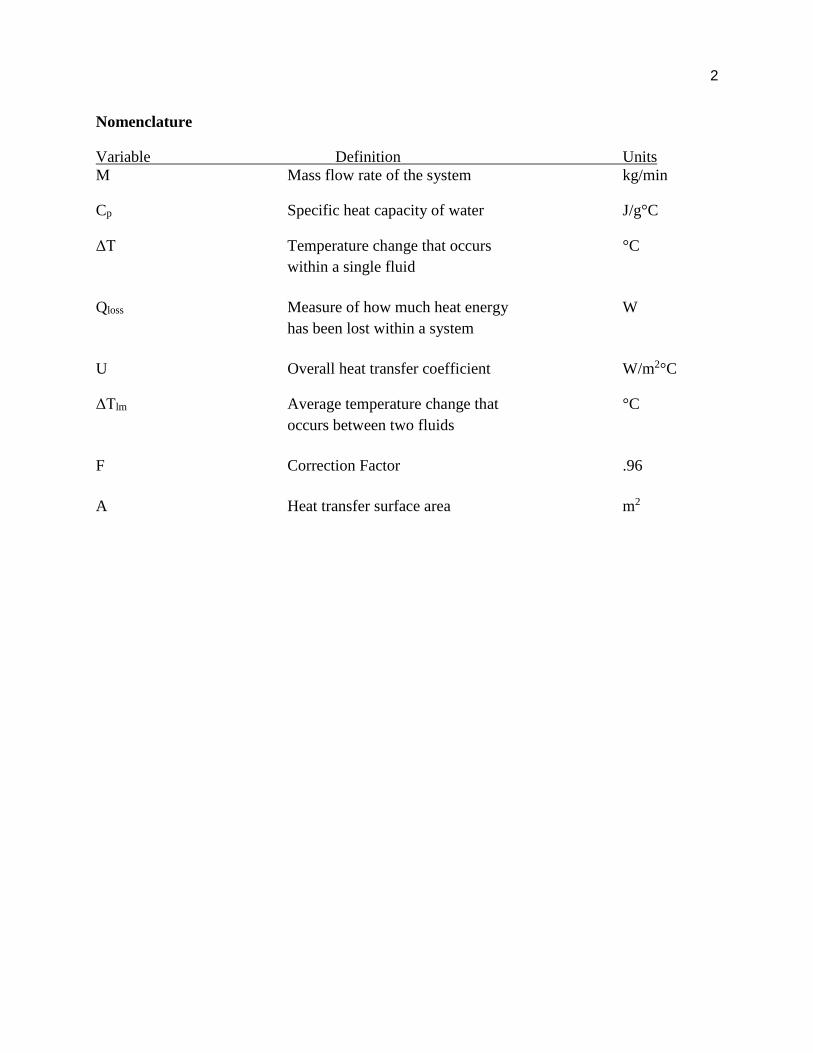
Nomenclature
Variable Definition Units
M Mass flow rate of the system kg/min
Cp Specific heat capacity of water J/g°C
ΔT Temperature change that occurs °C
within a single fluid
Qloss Measure of how much heat energy W
has been lost within a system
U Overall heat transfer coefficient W/m2°C
ΔTlm Average temperature change that °C
occurs between two fluids
F Correction Factor .96
A Heat transfer surface area m2
3
1.0 Introduction and Background
Heat exchangers are a vital part of chemical engineering process designs. To illustrate, in
prototype testing, an inventor discovers that his new device is prone to overheating, even though
heat sinks are already installed to provide cooling to the system. To solve this problem, the
engineer decides to install a heat exchanger into the system. A heat exchanger is a device that is
commonly used when heat sinks alone cannot prevent a device from overheating [1]. The most
well-known application of heat exchangers are car radiators. Radiators use antifreeze to transfer
heat energy from the engine, to the air surrounding the car [1].
There are many different types of heat exchangers, each having various applications. Three
examples include regenerative, plate, and shell and tube heat exchangers. Regenerative heat
exchangers are a unique type of heat exchanger that are used to maintain a temperature, rather than
vary it. In order to achieve this, initial thermal energy from a fluid is used to reheat that same fluid
as it loses its thermal energy throughout the process. Due to the nature of this heat exchanger, very
little external energy is required to maintain the overall temperature of the heat exchanger.
Conversely, plate heat exchangers have many thin plates inside with small gaps between each
plate. Alternating fluid then flows through each gap, causing the two fluids to exchange thermal
energy. This type of heat exchanger can be used to either cool, or heat a fluid. Plate heat exchangers
are commonly used in household refrigerators [2]. Similar to a plate heat exchanger, a shell and
tube heat exchanger utilizes two separate fluids to transfer thermal energy from one to the other.
To achieve this, one fluid is routed through a tube inside a hollow shell. The shell has the second
fluid flowing through it, allowing heat to transfer between the two.
Shell and tube heat exchangers are used widely in many different chemical processes
because of their numerous advantages. Shell and tube heat exchangers are capable of having a
large surface area for heat transfer to take place. This is because of their numerous tubes. This
design also minimizes the necessary overall length [3]. Shell and tube heat exchangers also offer
a lot of versatility when it comes to operating pressure and temperature. Since there are limited
pressure and temperature restrictions, small shell and tube heat exchangers can accommodate a
higher heat duty. This is because additions can be made to neglect thermal expansion effects as
well as variations to the thickness of the exchanger [4]. From a design perspective, the thickness
4
is easily varied, making them very adaptable. The number of tubes and different types of baffles
needed can be designed and implemented based off of specific operation conditions [4].
One of the main concerns with shell and tube heat exchangers is they are susceptible to
vibration problems caused from the fluid flowing throughout the pipes. Although the baffles
within the system help hold these tubes in place to reduce vibrations, problems can still arise [3].
Another concern is the maintenance of the tubes, which can be difficult. Because of this, fouling
can occur. Buildup can greatly affect the overall heat transfer coefficient and efficiency of the unit
[3]. When assessing these issues, observations of the heat energy gained or lost by the system must
be accomplished. For this experiment the equation used to determine this energy is
Q=MCpΔT.
(1)
M is the mass flow rate of the water, and is a measure of the flow of water into the system. In order
for proper calculations, data must be collected when the system is at steady state. Cp is the specific
heat capacity of the material, which is the amount of energy per unit mass required to raise the
temperature of a substance by one degree. ΔT is the change in temperature of the fluid throughout
the system.
This calculation is done for the cold and hot side of the heat exchanger to obtain Qcold and
Qhot. To determine the efficiency of the unit, the equation
Qhot= Qcold + Qloss
(2)
can be used to determine Qloss. This quantity will determine how much heat has been lost during
the experiment. Since the shell-side is the hot side, some of the energy escapes through conduction
to the outside environment, contributing to this value. For an efficient system, Qloss should be
minimized.
Another calculation used when analyzing heat exchange is calculating heat transfer
between two elements. The equation used is
Q = UAΔTlmF.
(3)
5
U is the overall heat transfer coefficient. This heat transfer coefficient is a function of the fluid
properties and material composition of the heat exchanger. U varies based on the design of the
heat exchanger. Q in this equation is calculated from Equation 1, and is the energy gained or lost
by the system. F is a correction factor that must be used for this heat exchanger to accommodate
for concurrent or parallel flow in the heat exchanger. In opposition, counter current flow occurs
when the streams are flowing in opposite directions. This leads to a constant flow of heat at each
point of contact and a higher rate of heat transfer. For this heat exchanger F is 0.96. A is the heat
transfer surface area for the tubes which is 50 square inches. ∆Tlm is the log mean temperature
difference and can be calculated by using the equation
(∆T2-∆T1)/ln(∆T2/∆T1)
(4)
where ∆T1 and ∆T2 are
∆T2 = T(hot, in) - T(cold,out),
(5)
and
∆T1 = T(hot,out) - T(cold,in).
(6)
The log mean temperature difference is unlike the other ∆T’s calculated in previous equations. It
is the temperature difference between two streams. In previous calculations, ∆T was simply the
temperature change over each single stream analyzed. Since in the system, temperatures are
constantly changing along a path, the log mean temperature difference is used to give an average
temperature gradient.
The two technical objectives of the experiment are to evaluate the effect of the tube-side
flow rate and shell-side flow rate on the steady-state heat duty and the overall heat transfer
coefficient of the heat exchanger. To accomplish this, flow rates were adjusted on one side, while
keeping the other side constant. The data used from steady state was used to determine how a
difference in flow rate affected the calculated values.
6
2.0 Experimental Methodology
2.1 Experiment and Apparatus:
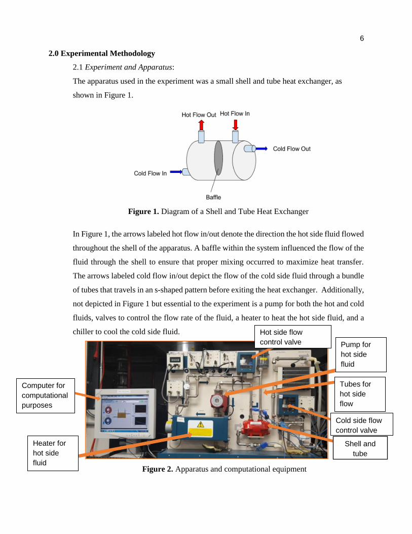
The apparatus used in the experiment was a small shell and tube heat exchanger, as
shown in Figure 1.
Figure 1. Diagram of a Shell and Tube Heat Exchanger
In Figure 1, the arrows labeled hot flow in/out denote the direction the hot side fluid flowed
throughout the shell of the apparatus. A baffle within the system influenced the flow of the
fluid through the shell to ensure that proper mixing occurred to maximize heat transfer.
The arrows labeled cold flow in/out depict the flow of the cold side fluid through a bundle
of tubes that travels in an s-shaped pattern before exiting the heat exchanger. Additionally,
not depicted in Figure 1 but essential to the experiment is a pump for both the hot and cold
fluids, valves to control the flow rate of the fluid, a heater to heat the hot side fluid, and a
chiller to cool the cold side fluid.
Figure 2. Apparatus and computational equipment
Shell and
tube
Tubes for
hot side
flow
Pump for
hot side
fluid
Computer for
computational
purposes
Heater for
hot side
fluid
Hot side flow
control valve
Cold side flow
control valve
7
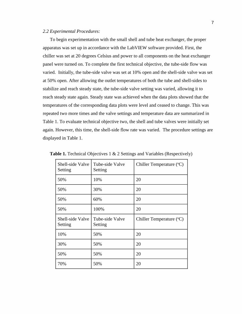
2.2 Experimental Procedures:
To begin experimentation with the small shell and tube heat exchanger, the proper
apparatus was set up in accordance with the LabVIEW software provided. First, the
chiller was set at 20 degrees Celsius and power to all components on the heat exchanger
panel were turned on. To complete the first technical objective, the tube-side flow was
varied. Initially, the tube-side valve was set at 10% open and the shell-side valve was set
at 50% open. After allowing the outlet temperatures of both the tube and shell-sides to
stabilize and reach steady state, the tube-side valve setting was varied, allowing it to
reach steady state again. Steady state was achieved when the data plots showed that the
temperatures of the corresponding data plots were level and ceased to change. This was
repeated two more times and the valve settings and temperature data are summarized in
Table 1. To evaluate technical objective two, the shell and tube valves were initially set
again. However, this time, the shell-side flow rate was varied. The procedure settings are
displayed in Table 1.
Table 1. Technical Objectives 1 & 2 Settings and Variables (Respectively)
Shell-side Valve
Setting
Tube-side Valve
Setting
Chiller Temperature (ºC)
50% 10% 20
50% 30% 20
50% 60% 20
50% 100% 20
Shell-side Valve
Setting
Tube-side Valve
Setting
Chiller Temperature (ºC)
10% 50% 20
30% 50% 20
50% 50% 20
70% 50% 20
8
3.0 Results
Two separate trials were conducted in this experiment, one varying the tube-side (cold side)
flow rate, and the other varying the shell-side (hot side) flow rate. In the first trial, the tube-side
flow rate was gradually increased, and the results have been presented in Table 2.
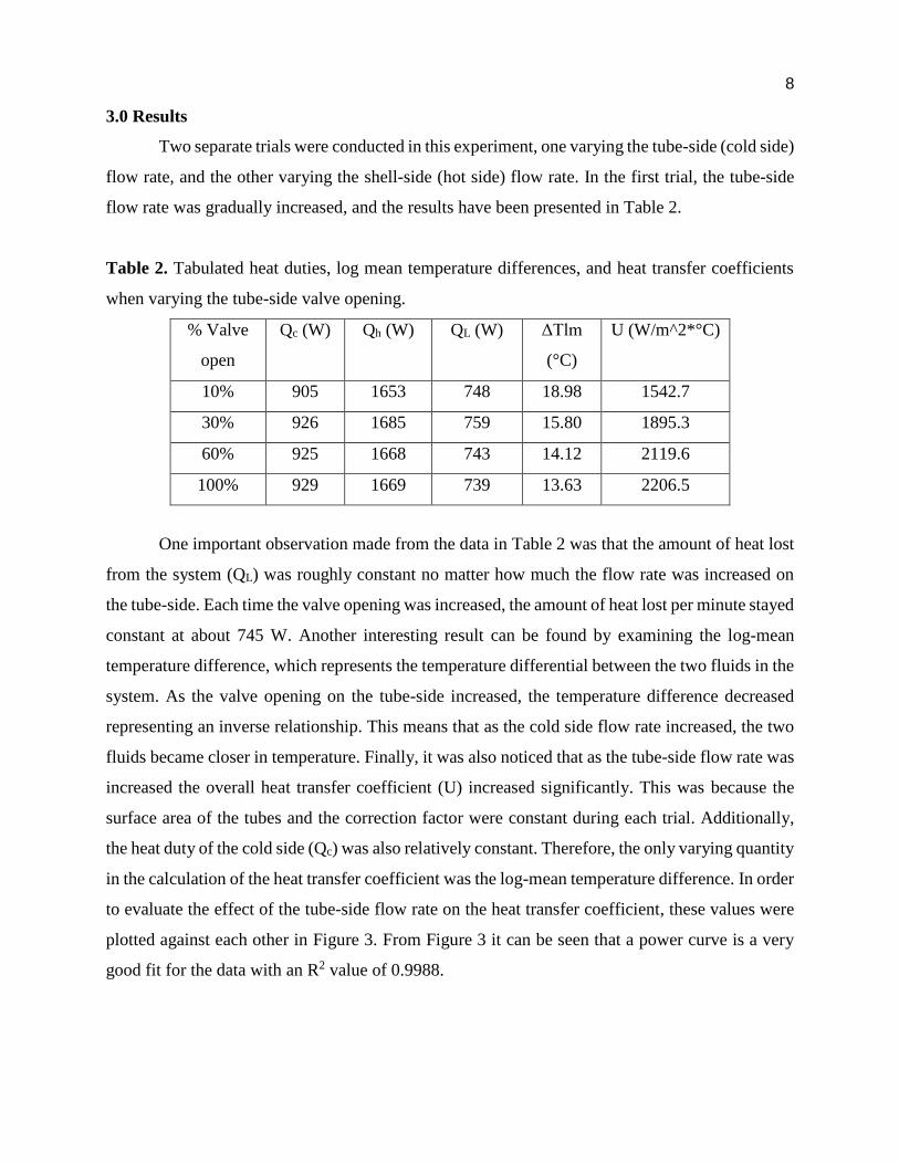
Table 2. Tabulated heat duties, log mean temperature differences, and heat transfer coefficients
when varying the tube-side valve opening.
% Valve
open
Qc (W) Qh (W) QL (W) ΔTlm
(°C)
U (W/m^2*°C)
10% 905 1653 748 18.98 1542.7
30% 926 1685 759 15.80 1895.3
60% 925 1668 743 14.12 2119.6
100% 929 1669 739 13.63 2206.5
One important observation made from the data in Table 2 was that the amount of heat lost
from the system (QL) was roughly constant no matter how much the flow rate was increased on
the tube-side. Each time the valve opening was increased, the amount of heat lost per minute stayed
constant at about 745 W. Another interesting result can be found by examining the log-mean
temperature difference, which represents the temperature differential between the two fluids in the
system. As the valve opening on the tube-side increased, the temperature difference decreased
representing an inverse relationship. This means that as the cold side flow rate increased, the two
fluids became closer in temperature. Finally, it was also noticed that as the tube-side flow rate was
increased the overall heat transfer coefficient (U) increased significantly. This was because the
surface area of the tubes and the correction factor were constant during each trial. Additionally,
the heat duty of the cold side (Qc) was also relatively constant. Therefore, the only varying quantity
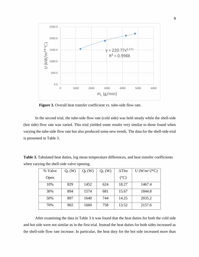
in the calculation of the heat transfer coefficient was the log-mean temperature difference. In order
to evaluate the effect of the tube-side flow rate on the heat transfer coefficient, these values were
plotted against each other in Figure 3. From Figure 3 it can be seen that a power curve is a very
good fit for the data with an R2 value of 0.9988.
9
Figure 3. Overall heat transfer coefficient vs. tube-side flow rate.
In the second trial, the tube-side flow rate (cold side) was held steady while the shell-side
(hot side) flow rate was varied. This trial yielded some results very similar to those found when
varying the tube-side flow rate but also produced some new trends. The data for the shell-side trial
is presented in Table 3.
Table 3. Tabulated heat duties, log mean temperature differences, and heat transfer coefficients
when varying the shell-side valve opening.
% Valve
Open
Qc (W) Qh (W) QL (W) ΔTlm
(°C)
U (W/m^2*C)
10% 829 1452 624 18.27 1467.4
30% 894 1574 681 15.67 1844.8
50% 897 1640 744 14.25 2035.2
70% 902 1660 758 13.52 2157.6
After examining the data in Table 3 it was found that the heat duties for both the cold side
and hot side were not similar as in the first trial. Instead the heat duties for both sides increased as
the shell-side flow rate increase. In particular, the heat duty for the hot side increased more than
y = 220.77x0.271
R² = 0.9988
0.0
500.0
1000.0
1500.0
2000.0
2500.0
0 1000 2000 3000 4000 5000 6000
U (
kW/m
2*°
C)
ṁc (g/min)
10
that for the cold side. However, when looking at the log-mean temperature difference, very similar
results were observed in both trials. After comparing the data in Table 2 and Table 3, it was noticed
that the ΔTlm values varied only within a few tenths of a degree Celsius between the two trials.
This means that the temperature difference between the two fluids in each trial was about the same
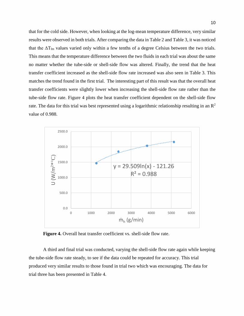
no matter whether the tube-side or shell-side flow was altered. Finally, the trend that the heat
transfer coefficient increased as the shell-side flow rate increased was also seen in Table 3. This
matches the trend found in the first trial. The interesting part of this result was that the overall heat
transfer coefficients were slightly lower when increasing the shell-side flow rate rather than the
tube-side flow rate. Figure 4 plots the heat transfer coefficient dependent on the shell-side flow
rate. The data for this trial was best represented using a logarithmic relationship resulting in an R2
value of 0.988.
Figure 4. Overall heat transfer coefficient vs. shell-side flow rate.
A third and final trial was conducted, varying the shell-side flow rate again while keeping
the tube-side flow rate steady, to see if the data could be repeated for accuracy. This trial
produced very similar results to those found in trial two which was encouraging. The data for
trial three has been presented in Table 4.
y = 29.509ln(x) - 121.26R² = 0.988
0.0
500.0
1000.0
1500.0
2000.0
2500.0
0 1000 2000 3000 4000 5000 6000
U (
W/m
2*°
C)
ṁh (g/min)
11
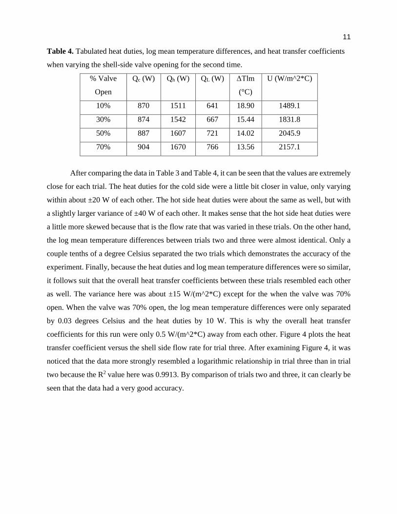
Table 4. Tabulated heat duties, log mean temperature differences, and heat transfer coefficients
when varying the shell-side valve opening for the second time.
% Valve
Open
Qc (W) Qh (W) QL (W) ΔTlm
(°C)
U (W/m^2*C)
10% 870 1511 641 18.90 1489.1
30% 874 1542 667 15.44 1831.8
50% 887 1607 721 14.02 2045.9
70% 904 1670 766 13.56 2157.1
After comparing the data in Table 3 and Table 4, it can be seen that the values are extremely
close for each trial. The heat duties for the cold side were a little bit closer in value, only varying
within about ±20 W of each other. The hot side heat duties were about the same as well, but with
a slightly larger variance of ±40 W of each other. It makes sense that the hot side heat duties were
a little more skewed because that is the flow rate that was varied in these trials. On the other hand,
the log mean temperature differences between trials two and three were almost identical. Only a
couple tenths of a degree Celsius separated the two trials which demonstrates the accuracy of the
experiment. Finally, because the heat duties and log mean temperature differences were so similar,
it follows suit that the overall heat transfer coefficients between these trials resembled each other
as well. The variance here was about ±15 W/(m^2*C) except for the when the valve was 70%
open. When the valve was 70% open, the log mean temperature differences were only separated
by 0.03 degrees Celsius and the heat duties by 10 W. This is why the overall heat transfer
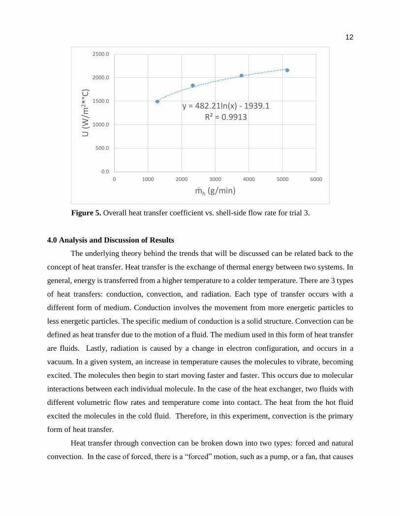
coefficients for this run were only 0.5 W/(m^2*C) away from each other. Figure 4 plots the heat
transfer coefficient versus the shell side flow rate for trial three. After examining Figure 4, it was
noticed that the data more strongly resembled a logarithmic relationship in trial three than in trial
two because the R2 value here was 0.9913. By comparison of trials two and three, it can clearly be
seen that the data had a very good accuracy.
12
Figure 5. Overall heat transfer coefficient vs. shell-side flow rate for trial 3.
4.0 Analysis and Discussion of Results
The underlying theory behind the trends that will be discussed can be related back to the
concept of heat transfer. Heat transfer is the exchange of thermal energy between two systems. In
general, energy is transferred from a higher temperature to a colder temperature. There are 3 types
of heat transfers: conduction, convection, and radiation. Each type of transfer occurs with a
different form of medium. Conduction involves the movement from more energetic particles to
less energetic particles. The specific medium of conduction is a solid structure. Convection can be
defined as heat transfer due to the motion of a fluid. The medium used in this form of heat transfer
are fluids. Lastly, radiation is caused by a change in electron configuration, and occurs in a
vacuum. In a given system, an increase in temperature causes the molecules to vibrate, becoming
excited. The molecules then begin to start moving faster and faster. This occurs due to molecular
interactions between each individual molecule. In the case of the heat exchanger, two fluids with
different volumetric flow rates and temperature come into contact. The heat from the hot fluid
excited the molecules in the cold fluid. Therefore, in this experiment, convection is the primary
form of heat transfer.
Heat transfer through convection can be broken down into two types: forced and natural
convection. In the case of forced, there is a “forced” motion, such as a pump, or a fan, that causes
y = 482.21ln(x) - 1939.1R² = 0.9913
0.0
500.0
1000.0
1500.0
2000.0
2500.0
0 1000 2000 3000 4000 5000 6000
U (
W/m
2*°
C)
ṁh (g/min)
13
the movement of fluids. In natural convection, heat transfer and the movement of fluid is caused
by differences in densities. The system in the experiment used pumps to create the flow of water
through the heat exchanger. Since the pumps are forcing the fluids to flow, a heat exchanger
utilizes forced convection to transfer the heat between the two fluids. The following will describe
the different trends that the provided theories support.
Between the trials, various trends can be noted. The primary trend deals with the log mean
temperature difference. In each trial, the log mean temperature difference decreased. In trial one,
it went from 18.98 ºC with a 10% tube-side valve opening to 13.36 ºC with a 100% tube-side valve
opening. Similarly in trial two, the log mean temperature difference decreased from 18.27 ºC with
a 10% shell-side valve opening to 13.52 ºC with a 70% shell-side valve opening. A third trial, that
mimicked trial two found similar results. When trial three was performed it was found that the log
mean temperature difference decreased from 18.90 ºC with a 10% shell-side valve opening to
13.56 ºC with a 70% shell-side valve opening. The reason for this decrease was because as the
volumetric flow rate of the hot and cold sides approached each other, the temperature differential
balanced equally. This trend was able to be observed in all trials because each trial was given
enough time for the heat transfer to reach equilibrium.
A second trend to be noted was with QL. In trial one, the QL remained constant at about
745 W. In trial two, the QL continued to increase from 624 W to 758 W. Likewise, in trial three,
the QL continued to increase from 641 W to 766 W. The major reason for the difference in QL was
due to the surroundings. In trial one, the cold side valve opening was increasing variably from 10%
to 100% as the hot side remained constant at 50% valve opening. As more cold water entered the
system, there was more cold fluid to absorb the constant flow of heat, allowing less heat to escape
to the environment. The reason for the variation of QL in trial two was due to the changing ratio of
cold to hot water in the heat exchanger. The cold side opening in trial two was fixed at 50% while
the hot side opening increased from 10% to 70%. Because of this, the cold side had roughly five
times more water flowing through the system than the hot side initially. This resulted in more heat
being transferred to the cold water and less being lost into the environment. However, as the hot
side valve opening increased, the ratio of cold to hot water decreased. This resulted in more heat
within the system, with a fixed amount of cold water. As a result, more heat escaped into the
environment, resulting in the rise of QL. This heat loss can also be observed in the hot side heat
duty of trials two and three. The hot side heat duty increased from 1452 W to 1660 W for trial two
14
and 1511 W to 1670 W for trial three. The more hot water added to the system, the more heat lost
to the environment.
The final trend that can be noted in the experiment was with the heat transfer coefficient
(U). The heat transfer coefficient is a quantitative characteristic of convective heat transfer
between a fluid medium and the surface the fluid flows over. U represents how well heat is
conducted by a medium. In theory, these U values should be equal to each other because the system
remained the same. According to the equation of the heat transfer coefficient, the heat duty for the
cold side, correction factor, surface area, and log mean temperature difference were the factors
that affected the coefficient. Since correction factor and surface area were constant in this
experiment, the heat duty for the cold side and log mean temperature difference were the only
factors influencing the coefficient. In trial one, there was little variation in the heat duty for the
cold side, meaning the log mean temperature significantly influenced U. However, in trials two
and three, U was affected by both the heat duty and log mean temperature difference, since the
heat duty for the cold side was observed changing. That is why the U observed throughout the
trials were slightly different. For example, U was 1542.7 W/m^2*°C*min when the tube-side valve
was opened 10% in trial one, 1467.4 W/m^2*°C*min when the shell-side valve was opened 10%
in trial two, and 1489.1 W/m^2*°C*min when the shell-side valve was opened 10% in trial three.
In finding that the data in trials one and two were adequate, trial three was performed just
as an extra run to “back up” the existing data. This, “back-up,” correctly showed that the data taken
was precise and accurate throughout the lab.
5.0 Summary and Conclusion
Ultimately, the goal of this experiment was to determine the effects of altering the flow
rates of a small shell and tube heat exchanger. The two technical objectives of the experiment
were to evaluate the effect of variations in flow of the cold, tube-side, and hot, shell-side of a
shell and tube heat exchanger. These changes were observed through the steady-state heat duty
and the overall heat transfer coefficient of the heat exchanger. From the results, it can be
concluded that as the flow rate of a shell and tube heat exchanger is altered, an effect on the heat
duties, log mean temperature difference, and the heat transfer coefficient can be observed. When
the cold side flow rate was incremented, the resulting heat duties for the cold side and hot side
increased proportionately, resulting in a constant Qloss. When the hot side flow rate was
15
incremented, both the heat duties of the cold side and hot side again increased, but the heat duty
of the hot side increased at a faster rate. This resulted in more energy lost. These results were
confirmed when trial three was run. Although, the slight increase of Qloss in trials two and three
did not have a noticeable effect on the log mean temperature difference and the heat transfer
coefficient trends. All three of the trials noticed a decrease of the log mean temperature
difference and an increase of the heat transfer coefficient as the flow rate for the heat exchanger
increased. This means that increasing flow allows for more heat to be transferred between the
two fluids.
These results can be very important when it comes to maximizing the efficiency of a shell
and tube heat exchanger. In order to achieve maximum efficiency, an engineer can take a
desired temperature needed and design the heat exchanger. By taking into account the size and
flow rate, the desired temperature can be reached while maximizing efficiency and reducing
costs. Since altering the flow rate effects the heat transfer as proven by this experiment, flow
rate is a vital part of the design in a shell and tube heat exchanger. Consequently, it is possible to
increase efficiency of a heat exchanger by increasing flow rate while decreasing the temperature
of the heating fluid in a case where a heat exchanger is used to increase the temperature of a
cooler fluid. This means that less energy would be needed to reach the necessary temperature of
the fluid being heated.
Therefore, the results from this experiment lead to information that will help to optimize
the shell and tube heat exchanger. Since heat exchangers are very common in industry,
designing a maximum efficiency heat exchanger at minimal costs will have a vast impact in
furthering the development of the industrial world.
16
6.0 Appendix
6.1 Steady State Data for All Trials
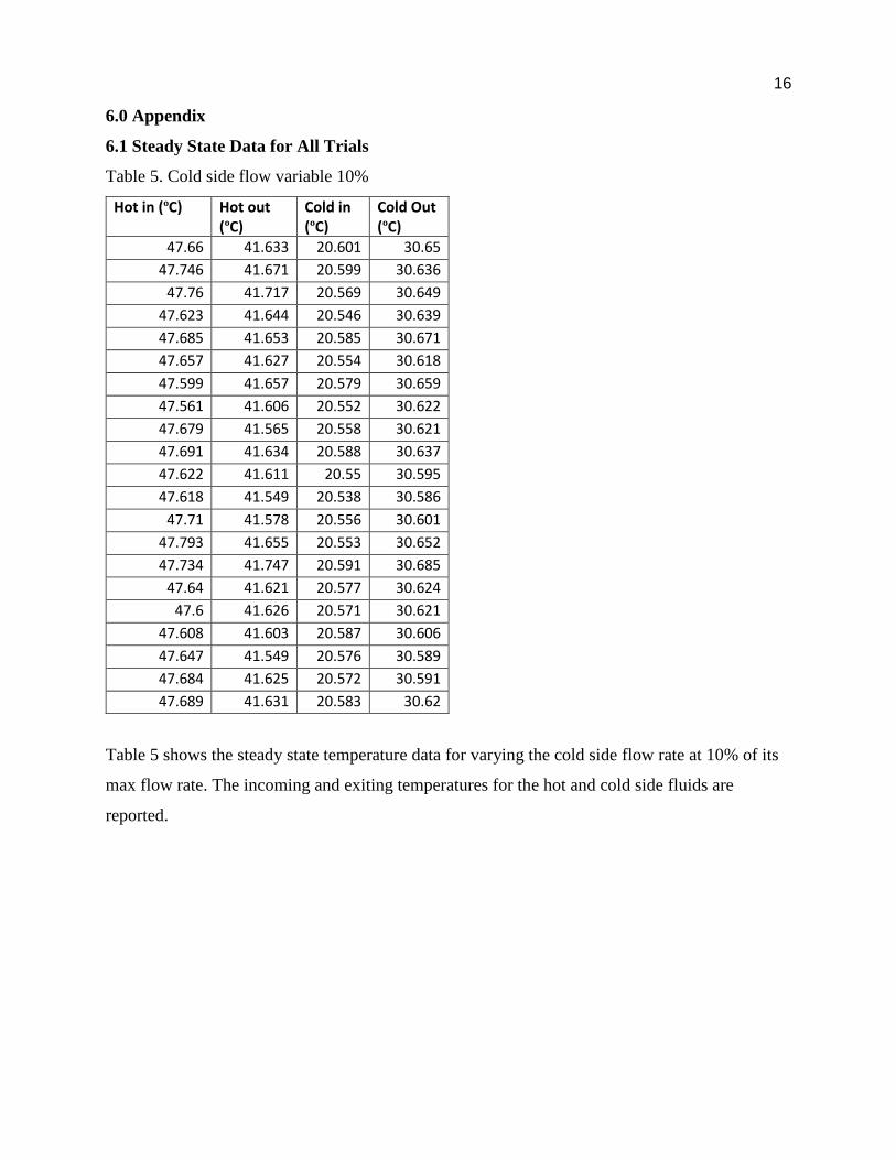
Table 5. Cold side flow variable 10%
Hot in (ºC) Hot out (ºC)
Cold in (ºC)
Cold Out (ºC)
47.66 41.633 20.601 30.65
47.746 41.671 20.599 30.636
47.76 41.717 20.569 30.649
47.623 41.644 20.546 30.639
47.685 41.653 20.585 30.671
47.657 41.627 20.554 30.618
47.599 41.657 20.579 30.659
47.561 41.606 20.552 30.622
47.679 41.565 20.558 30.621
47.691 41.634 20.588 30.637
47.622 41.611 20.55 30.595
47.618 41.549 20.538 30.586
47.71 41.578 20.556 30.601
47.793 41.655 20.553 30.652
47.734 41.747 20.591 30.685
47.64 41.621 20.577 30.624
47.6 41.626 20.571 30.621
47.608 41.603 20.587 30.606
47.647 41.549 20.576 30.589
47.684 41.625 20.572 30.591
47.689 41.631 20.583 30.62
Table 5 shows the steady state temperature data for varying the cold side flow rate at 10% of its
max flow rate. The incoming and exiting temperatures for the hot and cold side fluids are
reported.
17
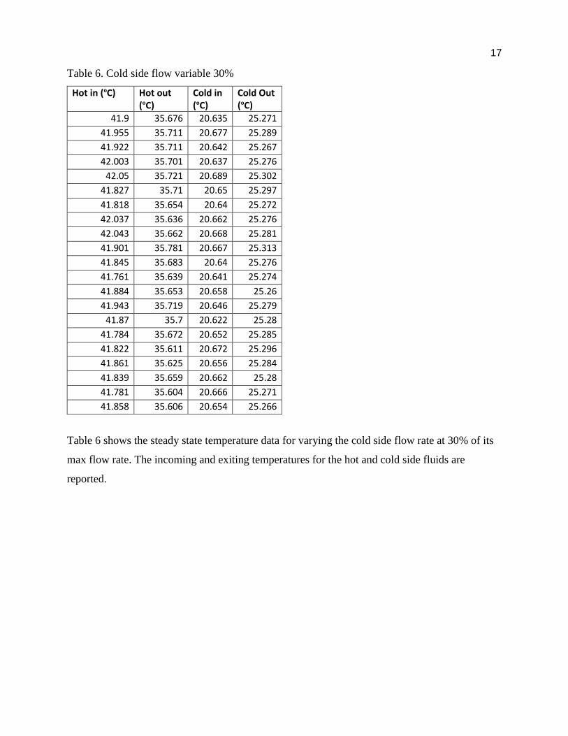
Table 6. Cold side flow variable 30%
Hot in (ºC) Hot out (ºC)
Cold in (ºC)
Cold Out (ºC)
41.9 35.676 20.635 25.271
41.955 35.711 20.677 25.289
41.922 35.711 20.642 25.267
42.003 35.701 20.637 25.276
42.05 35.721 20.689 25.302
41.827 35.71 20.65 25.297
41.818 35.654 20.64 25.272
42.037 35.636 20.662 25.276
42.043 35.662 20.668 25.281
41.901 35.781 20.667 25.313
41.845 35.683 20.64 25.276
41.761 35.639 20.641 25.274
41.884 35.653 20.658 25.26
41.943 35.719 20.646 25.279
41.87 35.7 20.622 25.28
41.784 35.672 20.652 25.285
41.822 35.611 20.672 25.296
41.861 35.625 20.656 25.284
41.839 35.659 20.662 25.28
41.781 35.604 20.666 25.271
41.858 35.606 20.654 25.266
Table 6 shows the steady state temperature data for varying the cold side flow rate at 30% of its
max flow rate. The incoming and exiting temperatures for the hot and cold side fluids are
reported.
18
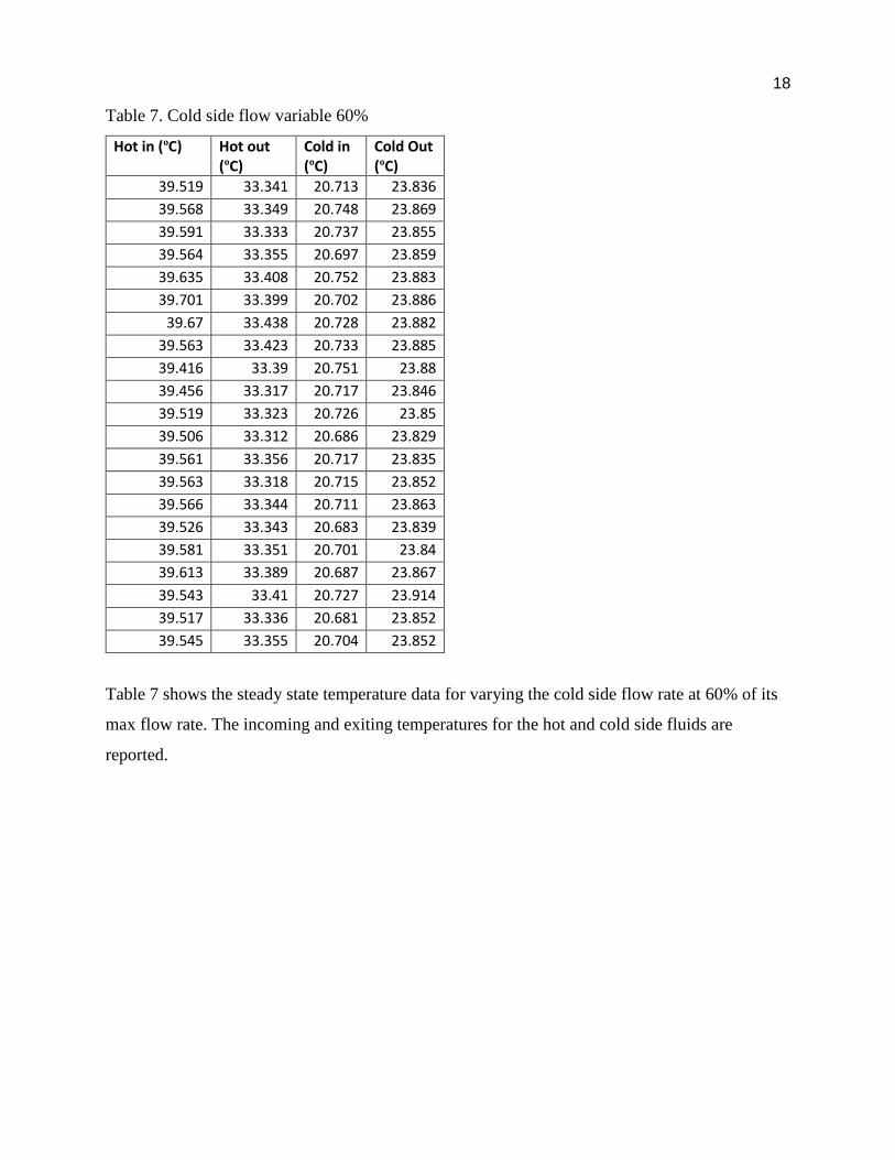
Table 7. Cold side flow variable 60%
Hot in (ºC) Hot out (ºC)
Cold in (ºC)
Cold Out (ºC)
39.519 33.341 20.713 23.836
39.568 33.349 20.748 23.869
39.591 33.333 20.737 23.855
39.564 33.355 20.697 23.859
39.635 33.408 20.752 23.883
39.701 33.399 20.702 23.886
39.67 33.438 20.728 23.882
39.563 33.423 20.733 23.885
39.416 33.39 20.751 23.88
39.456 33.317 20.717 23.846
39.519 33.323 20.726 23.85
39.506 33.312 20.686 23.829
39.561 33.356 20.717 23.835
39.563 33.318 20.715 23.852
39.566 33.344 20.711 23.863
39.526 33.343 20.683 23.839
39.581 33.351 20.701 23.84
39.613 33.389 20.687 23.867
39.543 33.41 20.727 23.914
39.517 33.336 20.681 23.852
39.545 33.355 20.704 23.852
Table 7 shows the steady state temperature data for varying the cold side flow rate at 60% of its
max flow rate. The incoming and exiting temperatures for the hot and cold side fluids are
reported.
19
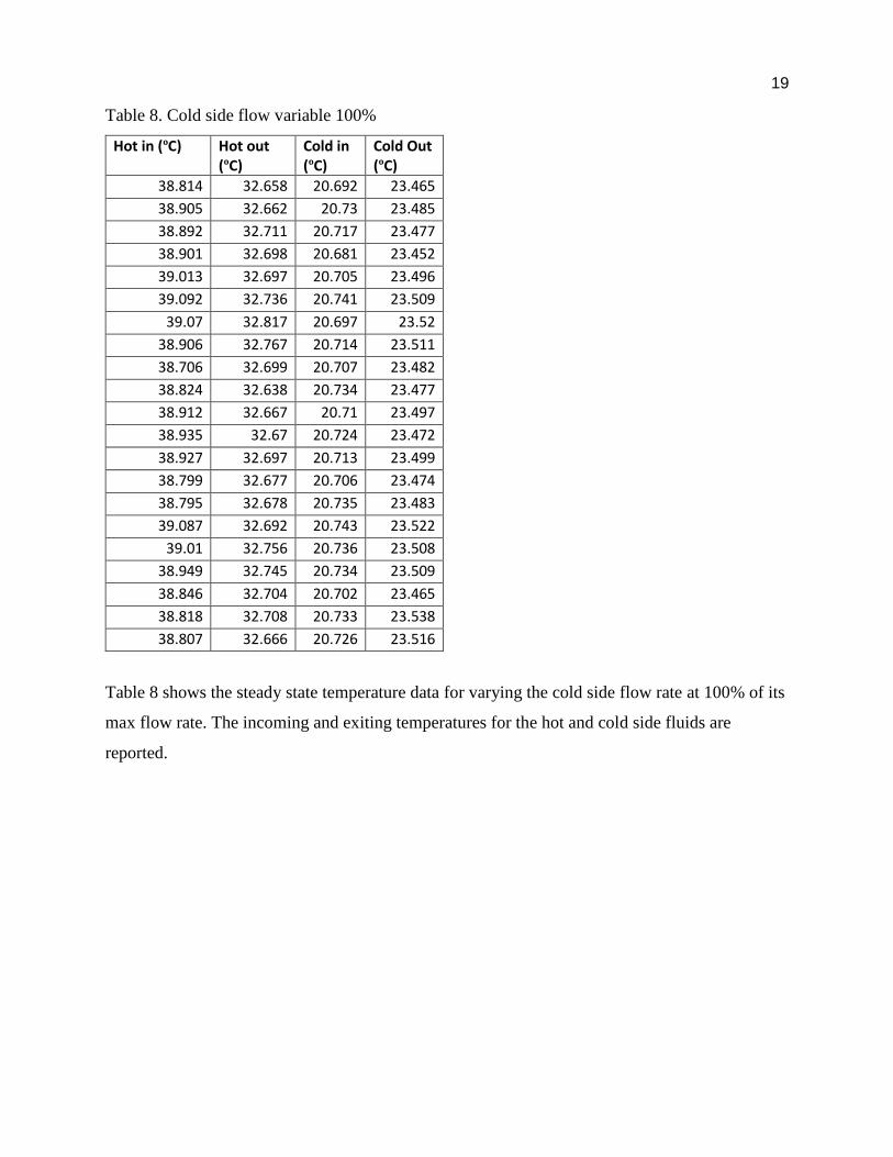
Table 8. Cold side flow variable 100%
Hot in (ºC) Hot out (ºC)
Cold in (ºC)
Cold Out (ºC)
38.814 32.658 20.692 23.465
38.905 32.662 20.73 23.485
38.892 32.711 20.717 23.477
38.901 32.698 20.681 23.452
39.013 32.697 20.705 23.496
39.092 32.736 20.741 23.509
39.07 32.817 20.697 23.52
38.906 32.767 20.714 23.511
38.706 32.699 20.707 23.482
38.824 32.638 20.734 23.477
38.912 32.667 20.71 23.497
38.935 32.67 20.724 23.472
38.927 32.697 20.713 23.499
38.799 32.677 20.706 23.474
38.795 32.678 20.735 23.483
39.087 32.692 20.743 23.522
39.01 32.756 20.736 23.508
38.949 32.745 20.734 23.509
38.846 32.704 20.702 23.465
38.818 32.708 20.733 23.538
38.807 32.666 20.726 23.516
Table 8 shows the steady state temperature data for varying the cold side flow rate at 100% of its
max flow rate. The incoming and exiting temperatures for the hot and cold side fluids are
reported.

20
Table 9. Hot side flow variable 10%
Hot in (ºC) Hot out (ºC)
Cold in (ºC)
Cold Out (ºC)
49.151 32.956 20.59 23.606
49.092 32.855 20.53 23.586
49.162 32.903 20.539 23.551
49.243 32.863 20.561 23.605
49.274 32.851 20.526 23.579
49.299 32.939 20.55 23.597
49.301 32.877 20.546 23.592
49.307 32.866 20.546 23.592
49.275 32.898 20.525 23.597
49.291 32.813 20.521 23.601
49.355 32.877 20.525 23.585
49.399 32.877 20.544 23.61
49.404 32.966 20.521 23.597
49.447 32.949 20.541 23.576
49.436 32.902 20.52 23.576
49.476 32.948 20.525 23.561
49.472 33.032 20.499 23.584
49.453 33.027 20.496 23.591
49.5 32.979 20.528 23.583
49.535 32.98 20.518 23.597
49.559 32.985 20.527 23.58
Table 9 shows the steady state temperature data for varying the hot side flow rate at 10% of its
max flow rate. The incoming and exiting temperatures for the hot and cold side fluids are
reported.

21
Table 10. Hot side flow variable 30%
Hot in (ºC) Hot out (ºC)
Cold in (ºC)
Cold Out (ºC)
42.774 33.316 20.591 23.863
42.773 33.315 20.589 23.842
42.915 33.297 20.617 23.886
42.872 33.298 20.585 23.855
42.843 33.274 20.581 23.89
42.979 33.285 20.607 23.866
42.982 33.334 20.581 23.879
42.93 33.367 20.597 23.887
42.915 33.383 20.588 23.871
42.948 33.398 20.592 23.887
42.903 33.407 20.597 23.868
42.901 33.333 20.604 23.905
42.852 33.376 20.625 23.889
42.898 33.31 20.59 23.884
42.941 33.326 20.623 23.901
42.876 33.373 20.608 23.883
42.948 33.341 20.619 23.895
42.933 33.365 20.643 23.904
42.864 33.355 20.623 23.879
42.946 33.348 20.61 23.868
42.914 33.368 20.614 23.894
Table 10 shows the steady state temperature data for varying the hot side flow rate at 30% of its
max flow rate. The incoming and exiting temperatures for the hot and cold side fluids are
reported.
22
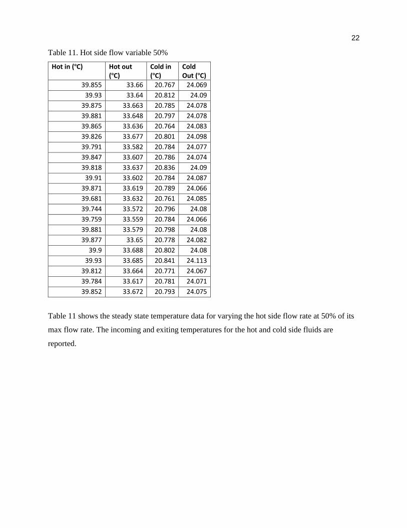
Table 11. Hot side flow variable 50%
Hot in (ºC) Hot out (ºC)
Cold in (ºC)
Cold Out (ºC)
39.855 33.66 20.767 24.069
39.93 33.64 20.812 24.09
39.875 33.663 20.785 24.078
39.881 33.648 20.797 24.078
39.865 33.636 20.764 24.083
39.826 33.677 20.801 24.098
39.791 33.582 20.784 24.077
39.847 33.607 20.786 24.074
39.818 33.637 20.836 24.09
39.91 33.602 20.784 24.087
39.871 33.619 20.789 24.066
39.681 33.632 20.761 24.085
39.744 33.572 20.796 24.08
39.759 33.559 20.784 24.066
39.881 33.579 20.798 24.08
39.877 33.65 20.778 24.082
39.9 33.688 20.802 24.08
39.93 33.685 20.841 24.113
39.812 33.664 20.771 24.067
39.784 33.617 20.781 24.071
39.852 33.672 20.793 24.075
Table 11 shows the steady state temperature data for varying the hot side flow rate at 50% of its
max flow rate. The incoming and exiting temperatures for the hot and cold side fluids are
reported.

23
Table 12. Hot side flow variable 70%
Hot in (ºC) Hot out (ºC)
Cold in (ºC)
Cold Out (ºC)
38.258 33.644 20.754 24.065
38.25 33.595 20.766 24.046
38.301 33.616 20.766 24.091
38.32 33.611 20.743 24.065
38.374 33.663 20.759 24.122
38.292 33.667 20.792 24.118
38.252 33.639 20.749 24.085
38.33 33.66 20.799 24.102
38.252 33.656 20.746 24.063
38.189 33.631 20.742 24.076
38.194 33.564 20.745 24.051
38.29 33.609 20.775 24.066
38.322 33.619 20.75 24.075
38.3 33.66 20.795 24.088
38.301 33.642 20.777 24.093
38.252 33.622 20.758 24.074
38.347 33.64 20.774 24.08
38.308 33.665 20.776 24.102
38.306 33.653 20.778 24.087
38.239 33.631 20.763 24.083
38.206 33.647 20.803 24.069
Table 12 shows the steady state temperature data for varying the hot side flow rate at 70% of its
max flow rate. The incoming and exiting temperatures for the hot and cold side fluids are
reported.

24
Table 13. Hot side flow variable 10%
Hot in (ºC) Hot out (ºC)
Cold in (ºC)
Cold Out (ºC)
49.151 32.956 20.59 23.606
49.092 32.855 20.53 23.586
49.162 32.903 20.539 23.551
49.243 32.863 20.561 23.605
49.274 32.851 20.526 23.579
49.299 32.939 20.55 23.597
49.301 32.877 20.546 23.592
49.307 32.866 20.546 23.592
49.275 32.898 20.525 23.597
49.291 32.813 20.521 23.601
49.355 32.877 20.525 23.585
49.399 32.877 20.544 23.61
49.404 32.966 20.521 23.597
49.447 32.949 20.541 23.576
49.436 32.902 20.52 23.576
49.476 32.948 20.525 23.561
49.472 33.032 20.499 23.584
49.453 33.027 20.496 23.591
49.5 32.979 20.528 23.583
49.535 32.98 20.518 23.597
49.559 32.985 20.527 23.58
Table 13 shows the steady state temperature data for varying the hot side flow rate at 10% of its
max flow rate. The incoming and exiting temperatures for the hot and cold side fluids are
reported. This is the data from a re-run of technical objective 2 and mimics that of Table 8.
25
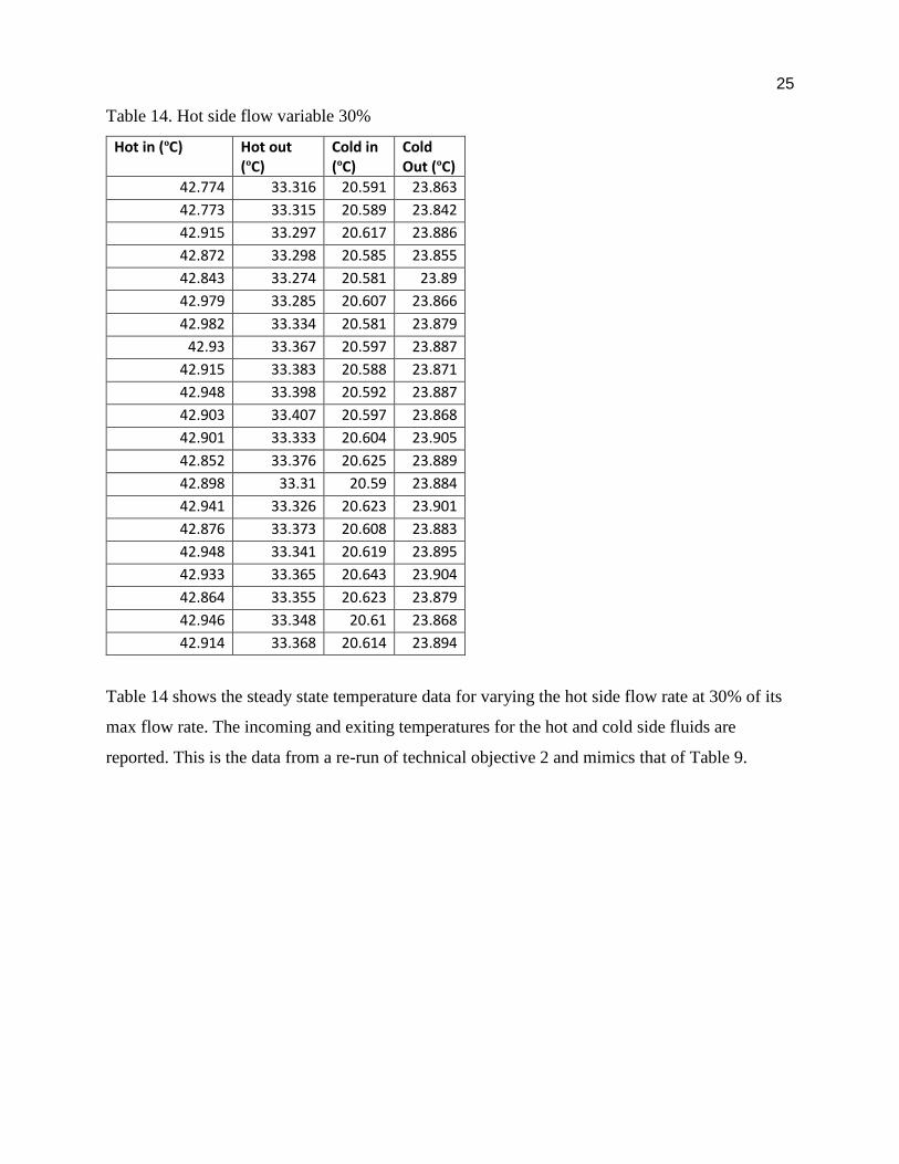
Table 14. Hot side flow variable 30%
Hot in (ºC) Hot out (ºC)
Cold in (ºC)
Cold Out (ºC)
42.774 33.316 20.591 23.863
42.773 33.315 20.589 23.842
42.915 33.297 20.617 23.886
42.872 33.298 20.585 23.855
42.843 33.274 20.581 23.89
42.979 33.285 20.607 23.866
42.982 33.334 20.581 23.879
42.93 33.367 20.597 23.887
42.915 33.383 20.588 23.871
42.948 33.398 20.592 23.887
42.903 33.407 20.597 23.868
42.901 33.333 20.604 23.905
42.852 33.376 20.625 23.889
42.898 33.31 20.59 23.884
42.941 33.326 20.623 23.901
42.876 33.373 20.608 23.883
42.948 33.341 20.619 23.895
42.933 33.365 20.643 23.904
42.864 33.355 20.623 23.879
42.946 33.348 20.61 23.868
42.914 33.368 20.614 23.894
Table 14 shows the steady state temperature data for varying the hot side flow rate at 30% of its
max flow rate. The incoming and exiting temperatures for the hot and cold side fluids are
reported. This is the data from a re-run of technical objective 2 and mimics that of Table 9.

26
Table 15. Hot side flow variable 50%
Hot in (ºC) Hot out (ºC)
Cold in (ºC)
Cold Out (ºC)
39.855 33.66 20.767 24.069
39.93 33.64 20.812 24.09
39.875 33.663 20.785 24.078
39.881 33.648 20.797 24.078
39.865 33.636 20.764 24.083
39.826 33.677 20.801 24.098
39.791 33.582 20.784 24.077
39.847 33.607 20.786 24.074
39.818 33.637 20.836 24.09
39.91 33.602 20.784 24.087
39.871 33.619 20.789 24.066
39.681 33.632 20.761 24.085
39.744 33.572 20.796 24.08
39.759 33.559 20.784 24.066
39.881 33.579 20.798 24.08
39.877 33.65 20.778 24.082
39.9 33.688 20.802 24.08
39.93 33.685 20.841 24.113
39.812 33.664 20.771 24.067
39.784 33.617 20.781 24.071
39.852 33.672 20.793 24.075
Table 15 shows the steady state temperature data for varying the hot side flow rate at 50% of its
max flow rate. The incoming and exiting temperatures for the hot and cold side fluids are
reported. This is a data from a re-run of technical objective 2 and mimics that of Table 10.
27
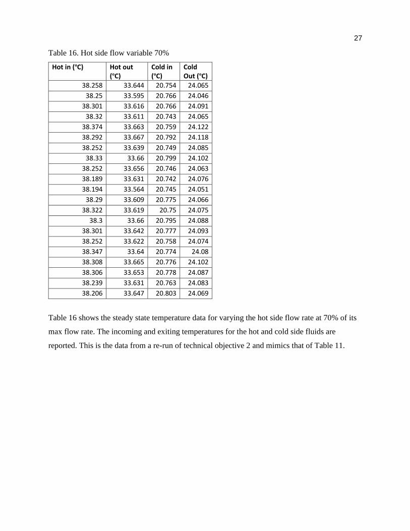
Table 16. Hot side flow variable 70%
Hot in (ºC) Hot out (ºC)
Cold in (ºC)
Cold Out (ºC)
38.258 33.644 20.754 24.065
38.25 33.595 20.766 24.046
38.301 33.616 20.766 24.091
38.32 33.611 20.743 24.065
38.374 33.663 20.759 24.122
38.292 33.667 20.792 24.118
38.252 33.639 20.749 24.085
38.33 33.66 20.799 24.102
38.252 33.656 20.746 24.063
38.189 33.631 20.742 24.076
38.194 33.564 20.745 24.051
38.29 33.609 20.775 24.066
38.322 33.619 20.75 24.075
38.3 33.66 20.795 24.088
38.301 33.642 20.777 24.093
38.252 33.622 20.758 24.074
38.347 33.64 20.774 24.08
38.308 33.665 20.776 24.102
38.306 33.653 20.778 24.087
38.239 33.631 20.763 24.083
38.206 33.647 20.803 24.069
Table 16 shows the steady state temperature data for varying the hot side flow rate at 70% of its
max flow rate. The incoming and exiting temperatures for the hot and cold side fluids are
reported. This is the data from a re-run of technical objective 2 and mimics that of Table 11.
28
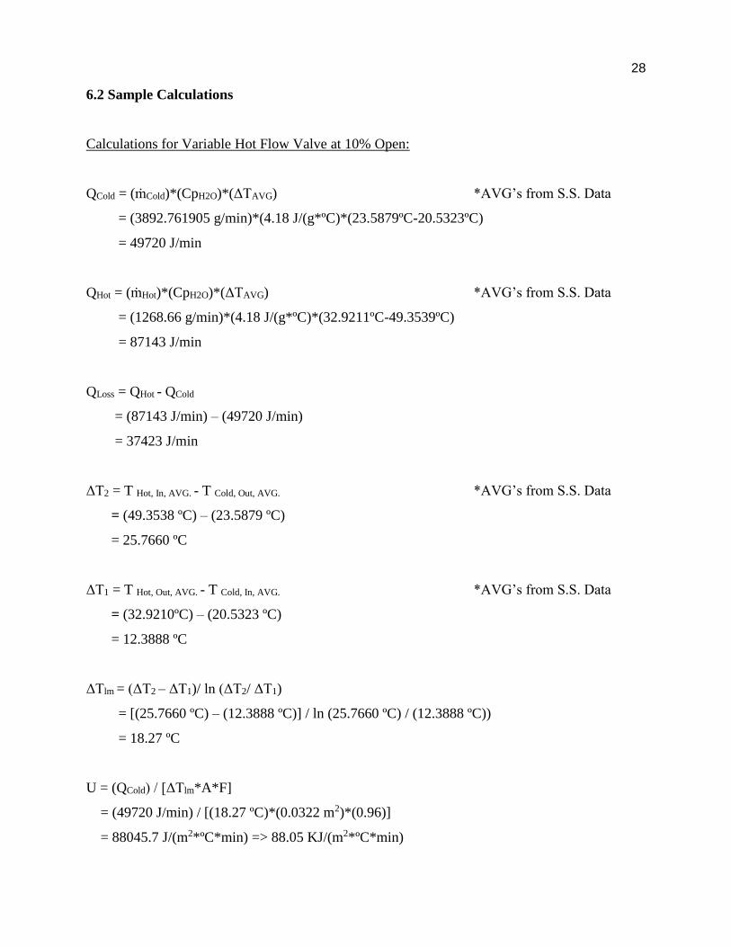
6.2 Sample Calculations
Calculations for Variable Hot Flow Valve at 10% Open:
QCold = (ṁCold)*(CpH2O)*(ΔTAVG) *AVG’s from S.S. Data
= (3892.761905 g/min)*(4.18 J/(g*ºC)*(23.5879ºC-20.5323ºC)
= 49720 J/min
QHot = (ṁHot)*(CpH2O)*(ΔTAVG) *AVG’s from S.S. Data
= (1268.66 g/min)*(4.18 J/(g*ºC)*(32.9211ºC-49.3539ºC)
= 87143 J/min
QLoss = QHot - QCold
= (87143 J/min) – (49720 J/min)
= 37423 J/min
ΔT2 = T Hot, In, AVG. - T Cold, Out, AVG. *AVG’s from S.S. Data
= (49.3538 ºC) – (23.5879 ºC)
= 25.7660 ºC
ΔT1 = T Hot, Out, AVG. - T Cold, In, AVG. *AVG’s from S.S. Data
= (32.9210ºC) – (20.5323 ºC)
= 12.3888 ºC
ΔTlm = (ΔT2 – ΔT1)/ ln (ΔT2/ ΔT1)
= [(25.7660 ºC) – (12.3888 ºC)] / ln (25.7660 ºC) / (12.3888 ºC))
= 18.27 ºC
U = (QCold) / [ΔTlm*A*F]
= (49720 J/min) / [(18.27 ºC)*(0.0322 m2)*(0.96)]
= 88045.7 J/(m2*ºC*min) => 88.05 KJ/(m2*ºC*min)

29
7.0 References
[1]Lytron Total Thermal Solutions. (2016). “What is a heat exchanger?”. Lytron Total Thermal
Solutions.(online article)
http://www.lytron.com/Tools-and-Technical-Reference/Application-Notes/What-is-a-Heat-
Exchanger
[2] Thomasnet.com. (2016). “Types of Heat Exchangers”. Thomas Publishing Company. (online
article)
http://www.thomasnet.com/articles/process-equipment/heat-exchanger-types
[3]Mahans Thermal Products. (2015). “Shell and Tube Heat Exchangers: Pros and Cons.” Mahns
Thermal Products. (online article).
https://heatexchangerswthdougleschan.wordpress.com/2014/12/28/types-of-heat-exchangers-
and-their-pros-and-cons/.
[4] H&C Heat Transfer Solutions. (2015). “Heat Exchanger Types and Selection.” H&C Heat
Transfer Solutions. (online Article). http://www.hcheattransfer.com/selection.html.