Smallholder Market Participation and Choice of Marketing Channel in the Presence of

Liquidity Constraints: Evidence from Zambian Maize Markets

Aakanksha Melkani,1 Nicole M. Mason,2 David L. Mather,3 Brian Chisanga, 4 and Thomas

Jayne5

Abstract

Smallholder farmers’ market participation in lucrative food grain markets is acknowledged as a

potential pathway towards agricultural commercialization and transformation of developing

economies. State run marketing boards often intervene in grain markets to help farmers access

fair prices for their product, especially in rural areas where markets are deemed to be highly

uncompetitive. However, smallholders’ participation in market as a seller, especially in staple

grain markets, is conditional on producing a marketable surplus beyond the households’

consumption needs. Constraints to production, such as the inability to invest in productivity-

enhancing agricultural inputs due to lack of liquidity during the production period, could inhibit

the production of a marketable surplus. In this article we study the selling behavior of

smallholder maize growers in Zambia during a period when Zambia’s parastatal marketing

board-Food Reserve Agency (FRA)-provided nationwide access to maize output markets at pan-

territorial prices that were higher than average market prices. We find that liquidity constrained

smallholders produced lower maize output, were less likely to sell maize, and less likely to sell to

the FRA, as compared to those who did not face liquidity constraints. The key takeaway is that

without adequate gains in productivity, market policies such as those of FRA are less likely to

benefit smallholders.

JEL codes: Q12, Q13, Q18, O13

Keywords: Liquidity; marketable surplus; market participation; maize; staple food grain; sub-

Saharan Africa; Zambia

1 PhD Student, Department of Agricultural, Food, and Resource Economics, Michigan State University 2 Associate Professor, Department of Agricultural, Food, and Resource Economics, Michigan State University 3 Assistant Professor, Department of Agricultural, Food, and Resource Economics, Michigan State University 4 Research Associate, Indaba Agricultural Policy Research Institute, Lusaka, Zambia 5 MSU Foundation Professor, Department of Agricultural, Food, and Resource Economics, Michigan State

University

This work was made possible by the generous support of the American People provided to the Feed the Future

Innovation Lab for Food Security Policy (FSP) through the United States Agency for International Development

(USAID) under Cooperative Agreement No. AID-OAA-L-13-00001 (Zambia Buy-In). This work was also

supported by the US Department of Agriculture (USDA), the National Institute of Food and Agriculture, Michigan

AgBioResearch [project number MICL02501], and Swedish International Development Agency (SIDA) funding to

IAPRI. The contents are the sole responsibility of the authors and do not necessarily reflect the views of FSP,

USAID, USDA, the United States Government, Michigan AgBioResearch, SIDA, IAPRI, or MSU. The authors of

this report also acknowledge helpful comments and insights from Scott Swinton, Jeffrey Wooldridge, Eduardo

Nakasone, Robert J. Myers, and Jason Snyder (each of whom are from MSU).

Introduction

Uncompetitive markets and poor market access are identified as important reasons for

limited market participation in agricultural markets by smallholder farmers in developing

countries (Goetz 1992; Key et al. 2000; Heltberg and Tarp 2002). This perspective, while well

supported by evidence, often overlooks the effect of constraints to production of a marketable

surplus on market participation as a seller. This is especially relevant for staple food grains

which are primarily grown for consumption and sale is conditional on the production of a surplus

beyond the household’s consumption needs. A major constraint faced by smallholders in

developing countries is the inability to invest adequately in crop productivity-enhancing inputs

due to lack of liquidity during the production period (Duflo et al. 2011; Kusunose, Mason-

Wardell, and Tembo 2020). This is known to reduce household’s agricultural production (Feder

et al. 1990; Foltz 2004; Winter-Nelson and Temu 2005) and consumption (Carter and Lybbert

2012) but there has not been a thorough investigation of its effect on smallholders’ ability to

participate in and benefit from lucrative agricultural output markets. In this article, we use

nationally representative panel data on Zambia’s maize growing smallholders to empirically test

the effect of liquidity constraints on maize marketing behavior. We find that, as compared to

unconstrained households, liquidity constrained households are indeed less likely to sell maize

and in case they do sell, they are less likely to take advantage of a marketing channel that offers

higher price but involves higher fixed cost.

Increased participation of smallholders in agricultural output markets can potentially shift

farmers from high-risk and low-productivity subsistence farming to more profitable commercial

agriculture (Timmer 1988; von Braun and Kennedy 1994; Heltberg and Tarp 2002), which in

turn can stimulate the rural economy of developing countries (Binswanger and von Braun 1991;

von Braun 1995). A first step in this direction is to increase their participation as sellers of staple

food grains. Most smallholders inevitably grow staples for household consumption and

investment in staple food production poses lower risk as compared to investment in cash crops or

other high value crops (Pingali et al. 2005; Jaleta et al. 2009). Yet, less than 50% of smallholder

farmers in many countries of sub-Saharan Africa (SSA) participate in staple food grain output

markets as sellers (see, e.g., Alene et al. 2008 for Kenya; Barrett 2008 for a survey of the

literature covering several countries in eastern and southern Africa; and Mather et al. 2013 for

Kenya, Mozambique and Zambia). In their pioneering work, de Janvry et al. (1991) explain that

low market participation by smallholders in agricultural markets is a household-specific market

failure that results from high transaction costs of accessing markets. Subsequent literature has

provided empirical evidence that high transaction costs arising from poor road infrastructure and

inadequate market information can reduce market participation (Goetz 1992; Key et al. 2000;

Heltberg and Tarp 2002). More recent evidence shows that improved access to public goods

(roads, extension, and communication services) and private assets (land, labor, animal traction)

can also facilitate market participation (Renkow et al. 2004; Cadot et al. 2006; Boughton et al.

2007). However, very few papers put this in perspective of imperfections in factor markets that

can undermine the capacity of a household to generate a marketable surplus (Alene et al. 2008;

Mather et al. 2013). We address some of this gap in literature by focusing on the liquidity

constraints faced by households during production period. Due to the seasonality of agriculture,

farmers have competing demands for cash received at the time of harvest, with meeting

consumption needs often being the most prominent (Stephens and Barrett 2011; Burke et al.

2019). This leaves limited resources to be spent on crop productivity-enhancing inputs (Duflo et

al. 2011; Dercon and Christiaensen 2011), which in turn is expected to reduce output supply and

thus the marketable surplus. The lack of well-functioning credit markets in many developing

countries further exacerbates this problem. While prior literature shows that liquidity constraints

lead to lower agricultural production (Feder et al. 1990; Foltz 2004; Winter-Nelson and Temu

2005), there is lack of rigorous research linking liquidity constraints during the production

period to market participation as a seller.6

Another less explored aspect of smallholder market participation in the developing

country context is the choice of marketing channel that households make when faced with

several buyer types, such as private traders of various scales, government agencies, and other

households in the community. The pioneering literature in this field has been dominated by

discussion of the choice to sell at the farmgate versus at a distant market and mostly limited to

commercial crops or largely commercialized markets (Fafchamps and Hill 2005; Shilpi and

6 The literature on smallholder grain market participation has extensively investigated a slightly different aspect of

the problem, i.e. the influence of liquidity constraints during the marketing period (i.e., after the marketable surplus

has been realized) to explain the “sell low, buy high" phenomenon (Stephens and Barrett 2011; Dillon 2017; Burke,

Bergquist, and Miguel 2019). Smallholder farmers are found to sell food grains relatively soon after harvest due to

cash constraints and/or lack of quality storage facilities. At this time of the year, food grain prices tend to be at their

lowest (i.e., “sell low”). Many of these households then purchase grain later in the marketing year, when grain prices

tend to be higher (i.e., “buy high”).

Umali-Deininger 2008; Zanello et al. 2014; Negi et al. 2018). In reality, households may face

several buyer types, each with their associated constraints and opportunities. Further, the

discussion of semi-commercialized food grain markets requires recognition of non-separability

of production and consumption decisions if there are multiple market failures. Muamba (2011)

and Takeshima and Winter-Nelson (2012) are the few papers that have studied the choice

between selling at the farmgate versus at a distant market when production and consumption

decisions are not separable. In this article, we examine whether the choice of marketing channel

is affected by liquidity constraints faced during the production period. We argue that liquidity

constraints will affect marketable surplus which in turn will affect the household’s ability to take

advantage of relatively more remunerative marketing channels.

The article makes four main contributions to literature. First, it generates quantitative

evidence about whether and to what extent liquidity constraints during the production period

affect food grain market participation and sellers’ choice of marketing channel. Second, it adds

to the thin literature on farmers’ marketing channel choice when production and consumption

(and thus marketing) decisions are non-separable. Third, it provides a rigorous conceptual

framework that helps understand the mechanisms through which liquidity constraints may affect

market participation and farmers’ choice of marketing channel and guides the specification of

our empirical model. Finally, this paper provides empirical evidence on the link between

constraints faced in agricultural production and accessing remunerative markets for agricultural

goods in developing country context.

We address the literature gaps noted above via econometric analysis of maize growing

smallholders from Zambia. Zambia has a considerably large agricultural sector that employs

49% of the country’s population (World Bank 2019a). Maize is the main staple food grain in

Zambia that is grown by almost all smallholder households and is an important source of income

for many of them (Chapoto et al., 2015); however, market participation in maize markets is far

from universal.7 Credit markets in rural Zambia are poorly developed. In the 2013/14 agricultural

season only 19% of rural households reported acquiring credit for agriculture from any formal or

informal source. In a recent experimental study conducted by Fink, Jack, and Masiye (2020) for

7 In the maize marketing years covered in this analysis (2011/12 and 2014/15), the percentage of maize growers who

sold more maize than they purchased (maize net sellers) was 52 and 42%, respectively.

rural Zambia, the authors find almost universal (98%) uptake of lean season loans at an implicit

interest rate of 4.5% per month, indicating severe cash needs among agricultural households.

Smallholders’ choice of marketing channel is of particular interest for Zambia given the

intervention by Zambia’s maize marketing board, Food Reserve Agency (FRA), in the domestic

maize market.8 The FRA bought maize from farmers at its depots throughout the country at a

pan-territorial price that was higher than the average market prices prevailing during the period

of study. Previous studies have shown that the FRA’s activities have raised the mean level and

reduced the variability of maize market prices (Mason and Myers 2013), which has induced

farmers to bring more land under maize cultivation (Mason, Jayne and Myers 2015). Its effects

on smallholder farmers’ welfare have, however, been less promising. The FRA’s activities have

been found to benefit net sellers who sell to FRA but have very limited spillover effects on the

remaining population and may in fact hurt rural net buyers of maize (Mason and Myers 2013;

Fung et al. 2020). One of the justifications for intervention in grain markets, by parastatals like

the FRA, is the presence of uncompetitive food markets and high transaction costs in remote

areas. However, recent evidence shows that the argument of widespread uncompetitive food

markets in rural SSA may be unsubstantiated and that market access has improved significantly

(Chamberlain and Jayne 2013; Sitko and Jayne 2014; Dillon and Dambro 2017). 9 On the other

hand, long payment delays by the FRA to farmers is a perennial problem as is the significant

uncertainty each year regarding the timing and scale of FRA’s maize purchases, making it a less

viable marketing channel for vulnerable and liquidity constrained households. The FRA has also

been criticized for crowding out private maize traders, who provide an essential service to

smallholders by providing timely maize market access and payments; and accounting for a large

share of the scarce government resources available for the agricultural sector (Jayne et al. 2011;

Sitko and Jayne 2014). Thus, this article has important implications for allocation of resources

and maize market policies pursued by the Zambian government.

8 The FRA is a parastatal that serves as a strategic food reserve and maize marketing board and seeks to raise and

stabilize maize market prices as a means of improving national food security and farmer incomes. During the period

of analysis for this study (2010-2015), the FRA played a major role in maize marketing in Zambia (see Figure D1 in

Appendix D) and purchased an average of 75% of the total volume of maize sold by smallholders each year (Fung et

al. 2020). 9 Sitko and Jayne (2014) find that even the remotest villages in Zambia were visited by at least one private maize

trader during the peak maize marketing season and that private traders made only small marketing margins through

maize transactions, an important indicator of competitive markets. Similarly, Chamberlain and Jayne (2013) find

that private trader activity was higher and distance travelled by smallholders for crop sales was lower in areas where

public marketing boards reduced their activity.

Conceptual Framework

We use the framework of a non-separable agricultural household model and assume that

production, consumption, and initial marketing decisions are made simultaneously at the time of

planting (Singh, Squire, and Strauss 1986; Key et al. 2000). However, once agricultural output

has been realized and harvest-time prices are revealed, the household can update its marketing

decisions.

Let a (potentially risk-averse) agricultural household maximize its expected utility of

consumption of maize (cmz), leisure (cl), and market-purchased goods (cmk), given household

level characteristics (zh) that affect consumption tastes and preferences and subject to several

constraints (See Appendix A for complete model). For simplicity, we assume maize to be the

only agricultural product produced by the household. We explicitly model liquidity constraints

during the production period and assume that the liquidity constraints apply only to the variable

production inputs (here: labor (l) and non-labor variable inputs (x)). Following de Janvry et al.

(1992), the input purchase liquidity constraint can be represented as, 𝜂(𝒑𝒙𝒙 + 𝑤𝑙 − 𝐾) = 0,

where w and px denote the prices of labor and non-labor inputs, respectively. is the shadow

price of liquidity and K represents the cash available with the household. Thus, for liquidity

constrained households (LC), liquidity is a binding constraint ((𝒑𝒙𝒙 + 𝑤𝑙 − 𝐾) = 0 𝑎𝑛𝑑 𝜂 > 0 )

and the amount of agricultural inputs used will be limited by some upper limit K. On the other

hand, if the household is not liquidity constrained (UC), the constraint is no longer binding

((𝒑𝒙𝒙 + 𝑤𝑙 − 𝐾) < 0 𝑎𝑛𝑑 𝜂 = 0) and purchases of inputs are not limited by K. LC and UC

households will then maximize their expected utility under different sets of constraints, and thus

have different input demand and output supply functions:

(1a) 𝒒𝑳𝑪 = 𝒒𝑳𝑪(𝑝𝑒, 𝒑𝒎𝒌, 𝑤(1 + 𝜂), 𝑝𝑥(1 + 𝜂), 𝐾, 𝒛𝒉, 𝒛𝒒)

(1b) 𝒒𝑼𝑪 = 𝒒𝑼𝑪(𝑝𝑒, 𝒑𝒎𝒌, 𝑤, 𝑝𝑥 , 𝒛𝒉, 𝒛𝒒)

Here, 𝒒𝑳𝑪 and 𝒒𝑼𝑪 denote the vector of input demand and output supply functions for LC

and UC households, respectively; pe is the household’s expectation, as of planting time, of the

maize price that will prevail at harvest time; pmk is the vector of prices for other market

purchased consumption goods, and zq is vector of fixed and quasi-fixed factors affecting

production. (1 + 𝜂) represents an implicit input price markup for households that are liquidity

constrained. An important implication of this result is that LC households would be using less

inputs and producing less output than unconstrained households, ceteris paribus (𝒒𝑳𝑪 < 𝒒𝑼𝑪 ).

Let pm be the realized price of maize at harvest and be household-specific transaction costs

involved in marketing maize such that >0. These transaction costs are added to the market

price of maize if the household is a buyer of maize and subtracted from the price of maize

received if the household is a seller of maize (Key et al. 2000). Thus, the household-specific

buyer and seller prices can be represented as pb = (pm + ) and ps = (pm – ), respectively. Let

𝑝𝑎(𝑞𝑚𝑧 ,∙) be the household’s shadow price of maize that is a function of the household’s maize

output (𝑞𝑚𝑧) and other household characteristics (∙). We assume that 𝑝𝑎(𝑞𝑚𝑧 ,∙) is a function

strictly decreasing in 𝑞𝑚𝑧. Thus, since LC households produce less maize output (𝑞𝑚𝑧 𝑙𝑐 < 𝑞𝑚𝑧

𝑢𝑐 ),

they would have a higher shadow price of maize than UC households (i.e., 𝑝𝑙𝑐 𝑎 > 𝑝𝑢𝑐

𝑎 ).

The household’s maize market position will be determined as follows: Household sells maize if

𝑝𝑠 ≥ 𝑝𝑎; household buys maize if 𝑝𝑏 ≤ 𝑝𝑎; household is autarkic with respect to maize if

𝑝𝑏 > 𝑝𝑎 > 𝑝𝑠. Based on this discussion, we state the following hypotheses:

Hypothesis 1: Liquidity-constrained maize-producing households are less likely to become maize

sellers, all else remaining constant, as compared to unconstrained households since

Pr[𝑝𝑙𝑐𝑎 ≤ 𝑝𝑠] < Pr[𝑝𝑢𝑐

𝑎 ≤ 𝑝𝑠].

Hypothesis 2: A liquidity-constrained household’s probability to sell maize will be less

responsive to changes in expected prices. We expect this because the liquidity constraint limits a

household’s capacity to increase production in response to higher expected prices, i.e.

∂ Pr[𝑝𝑙𝑐𝑎 ≤𝑝𝑠]

∂𝑞𝑚𝑧𝑙𝑐 .

∂𝑞𝑚𝑧𝑙𝑐

∂𝑝𝑒<

Pr[𝑝𝑢𝑐 𝑎 ≤ 𝑝𝑠]

∂𝑞𝑚𝑧𝑢𝑐 .

∂𝑞𝑚𝑧𝑢𝑐

∂𝑝𝑒 , because

∂𝑞𝑚𝑧𝑙𝑐

∂𝑝𝑒<

∂𝑞𝑚𝑧𝑢𝑐

∂𝑝𝑒.

The third hypothesis links liquidity constraints during the production period with the

marketing channel chosen by maize sellers. Similar to the case of market position, we assume

that the choice of marketing channel is determined after maize output has been realized. Further,

we assume that the choice of marketing channel is conditional on the decision to participate in

the maize market as a seller. We continue to assume (as we did above) that the household is

potentially risk-averse and thus motivate the problem from an expected utility maximization

perspective instead of a profit maximization one. Let 𝑉𝑗(𝑝𝑗𝑠𝑚 − 𝐹𝑗; 𝒛𝒉) be the expected utility

obtained from selling to marketing channel j. Here, 𝑝𝑗𝑠 represents the effective price received

from selling maize to channel j. The effective price incorporates transaction costs incurred in

transporting and handling per unit of maize and also discounts the price by the expected delay in

market entry and/or in payment by the buyer. m is the quantity of maize marketed by household

to channel j. 𝐹𝑗 is a fixed transaction cost associated with use of channel j. This may include

search and negotiation costs specific to that channel, such as membership of a cooperative or

farmer group that facilitates the collection and transport of maize in bulk from the village to

market or FRA depot, and uncertainty related to specific channels (like the FRA). This

essentially implies that to be able to sell to channel j, a household must be marketing enough

maize such that 𝑝𝑗𝑠𝑚 > 𝐹𝑗 , ceteris paribus. If 𝐹𝑗 is higher for a channel j, a higher effective price

(𝑝𝑗𝑠) or marketable surplus (m) will be required to compensate for the higher fixed cost. Given

this background we state our third hypothesis as follows:

Hypothesis 3: Since LC households are expected to be producing a smaller marketable surplus

(𝑞𝑚𝑧 𝑙𝑐 < 𝑞𝑚𝑧

𝑢𝑐 ), they are less likely to be able to overcome high fixed costs incurred in selling to

channels such as the FRA, i.e., Pr[𝑉𝐹𝑅𝐴 − 𝑉𝑗 > 0|𝐿𝐶] < Pr[𝑉𝐹𝑅𝐴 − 𝑉𝑗 > 0|𝑈𝐶], where j is

any other marketing channel.

Data

The main data source used in this analysis is the Rural Agricultural Livelihoods Survey

(RALS), a three-wave nationally representative panel survey dataset of smallholder farm

households in Zambia. We utilize the first and second waves of the RALS data.10 These waves

were implemented in June-July of 2012 and 2015, respectively, by the Indaba Agricultural

Policy Research Institute (IAPRI) in collaboration with the Zambian Central Statistical Office

(CSO) and the Ministry of Agriculture (MoA). See CSO (2012) for details on the RALS sample

design. The dataset contains detailed information on household demographics, crop and livestock

production and marketing, off-farm employment and own business activities, distances to roads,

markets, and public services. The 2012 survey covered the 2010/11 agricultural year (October

2010–September 2011) and the associated crop marketing year (May 2011–April 2012). The

2015 survey covered the 2013/14 agricultural year and the 2014/15 crop marketing year.

A total of 8,839 households were interviewed in the 2012 RALS. Of these, 7,254 (82%) were

successfully re-interviewed in 2015. Our analytical sample consists of the balanced panel of

6,063 RALS households that grew maize in both 2012 and 2015, which amounts to a total of

10 Data from the third wave, which was conducted in June-July 2019, were not available for analysis at the time of

this study.

12,126 households (84% of the total balanced sample and 73% of the total households surveyed).

Tests for attrition bias based on a procedure recommended by Wooldridge (2010) fail to reject

the null of no attrition bias for all dependent variables except one. We suspect that this exception

may be due to our inability to control for unobserved heterogeneity in the tests (which we

otherwise control for in all our main analysis). Thus, we do not consider attrition bias to be a

major cause of concern for our analysis. Details of the attrition test can be found in Appendix B.

The explanatory variables obtained from RALS are briefed here. The price of inorganic fertilizer

and seed and agricultural wage rate (the price to weed 0.25 ha) are used to control for

agricultural input prices (px and w in the conceptual framework). These prices were recorded at

the household level in the RALS but we compute district level medians to remove outliers and

alleviate concerns about incidental truncation (fertilizer prices were only captured for households

that used fertilizer). Distances to important points of market access such as the nearest paved and

unpaved roads, and agricultural market are used as proxies for transaction costs ( ). We also

include the number of maize traders that arrived in the village during the peak maize marketing

season (May-October) to capture the competitiveness and market access within the village (as

suggested by Chamberlain and Jayne (2013) and Sitko and Jayne (2014)). Dummy variables that

indicate the household's ownership of a bicycle, radio, and cellphone are included to represent

the household's capacity to reduce fixed transaction costs such as those associated with obtaining

price and buyer information. Land, livestock (measured as tropical livestock units (TLUs)), and

number of plows, harrows, and ox-carts owned by the household are used to control for the

household’s quasi-fixed factors of production (𝒛𝒒).11 Controls for household characteristics

affecting consumption (𝒛𝒉) include household size (the number of full-time adult equivalent

household members) and various characteristics of the household head (age, education, and sex).

We use district-level data on retail maize prices collected by the CSO (CSO 2018) to compute

maize market prices. Even though the RALS records price data for each maize transaction made

by a household, we refrain from using this information to avoid bias due to incidental

truncation.12 Maize market prices in Zambia are also significantly affected by the government’s

11 TLU’s were calculated with the following FAO formula: cattle = 0.70, sheep and goats = 0.10, pigs = 0.20 and

chickens = 0.01 (FAO 2007). 12 Since the price information in RALS was only recorded for households that sold maize, these prices may not

accurately reflect the prices faced by all households. The resulting measurement errors may in turn be systematically

correlated with unobservables that determine market participation.

market interventions through the FRA (Mason and Myers 2013). We do not explicitly model the

interdependence of market and FRA prices; rather we include separate variables for the FRA and

market prices. For each of these, we compute estimates of each household’s expected (𝑝𝑒) and

realized post-harvest maize price (𝑝𝑚). For computing expected maize price we assume that

households make the naïve expectation that next period’s prices will be similar to last period’s

prices. Thus, we use the market price as of August of the marketing season just before the

agricultural season as the expected market price of maize.13 Similarly, the FRA price during the

previous marketing year is used as a proxy for a household’s expected FRA price. On the other

hand, the district-level maize retail price in August of each harvest year is used as the realized

post-harvest maize market price. The post-harvest FRA price is simply that paid by the FRA

during each harvest year. All prices are adjusted to household level transport costs (obtained

from the RALS) to generate farmgate prices. See Appendix C for further details on the

computation of prices.

Rainfall is an important determinant of agricultural production in the context of Zambia

where smallholder agriculture is almost exclusively rainfed. Thus, we include information on

rainfall and moisture shock during the growing season as well as their long-term averages (a 16-

year moving average).14 A moisture shock in the season before the planting season of interest

was used as the exclusion restriction for liquidity status. These variables were obtained from data

compiled by Snyder et al. (2019) using geospatial data from Tropical Applications of

Meteorology using Satellite data and ground-based observations (TAMSAT) (Maidment et al.

2014; Tarnavsky et al. 2014; Maidment et al. 2017). Snyder et al. (2019) matched the TAMSAT

data to GPS locations of RALS households and created rainfall estimates using the Raster

Calculator tool in ArcGIS Model Builder. The TAMSAT data has a spatial resolution of

approximately 0.0375 x 0.0375 degrees, which is approximately 4 x 4 kilometers, or 16 square

13 Zambia’s marketing season runs from May to April and agricultural season runs from October to September.

Thus, the expected prices as of October, 2010 would be the market price of maize as of August, 2010. We used the

prices as of August because in our sample the largest share of maize transactions (46%) were made during the month

of August, followed by July (20%) and September (14%). It could be a matter of concern that August prices do not

represent the true price faced or expected by the household. We conduct sensitivity analysis using two other

measures of prices. These are discussed later in the article. 14 Moisture shock here is defined as the presence of more than one moisture stress period during the maize growing

season. Moisture stress is defined as in Snyder et al. (2019) as the number of overlapping 20-day periods with less

than 40 mm of rainfall. Kusunose et al. (2020) use a similar weather shock variable as an instrument for liquidity.

kilometers (Snyder et al. 2019). In practical terms, these estimates are therefore village-level

measures.

Finally, the consumer price index from the World Bank (2019b) was used to convert all

prices from nominal to real terms (with base year 2017=100). This implicitly controls for

variation in the prices of consumer goods (𝒑𝒎𝒌). Descriptive statistics for all variables can be

found in the table D1 of Appendix D.

Important definitions

In this section we describe three variables that are an integral part of the analysis: the

household’s liquidity status during the production period, their maize market position, and the

maize marketing channel chosen by net sellers for their largest transaction.

Liquidity status

Liquidity is a difficult concept to measure because it is not easily observable. It is often

also confused with a similar but slightly different concept of credit constraint/access (Winter-

Nelson and Temu, 2005). Further, different types of liquidity constraints can affect different

household decisions, such as, production of farm and non-farm goods and consumption of

market and home-produced goods (Sadoulet and de Janvry 1995). In this article, liquidity

constraints imply lack of readily available cash in adequate amount to enable the household to

invest in productivity enhancing agricultural inputs. We follow an approach similar to Winter-

Nelson and Temu (2005) and exploit unique data available in RALS to define a household to be

liquidity constrained during the production period if one or both of the following conditions are

met: (1) The household claims to not have acquired fertilizer from the market due to a lack of

cash; and/or (2) the household claims to not have obtained fertilizer from the Farmer Input

Support Program (FISP) due to – (a) not being able to afford the farmer’s down payment for

obtaining fertilizer through FISP, and/or (b) lack of cash for the mandatory cooperative

membership payment required for participation in the program.15, 16

15 FISP is a large-scale government program designed to enable eligible farmers to obtain farm at subsidized prices.

Eligibility is primarily determined by landholding, membership in a farmer cooperative and payment for part of the

cost for inputs received (Mason, Jayne, and Mofya-Mukuka 2013). During the study period, the program focused on

maize inputs (inorganic fertilizer and improved seed). Since the 2015/16 agricultural year, the FISP has been

partially converted into a flexible electronic voucher program (Kuteya, Chinmaya, and Malata 2018) with aims to

crowd-in private sector participation in Zambia’s agricultural input value chains and give farmers more flexibility in

terms of the farm inputs or equipment for which they can use the e-voucher. 16 According to Burke, Jayne, and Sitko (2012) the cash outlays required for obtaining inputs from FISP could cost

up to 20% of the annual gross income for 60% of the smallholders in Zambia, thus precluding many smallholders

A natural concern with a stated preference measure of liquidity such as the one used here

is hypothetical bias – i.e., households overstating the liquidity constraints that they face. It may

be that households imprecisely state other constraints, such as poor returns to or low profitability

of fertilizer use, that keep them from purchasing fertilizer as ‘lack of cash’. We alleviate these

concerns through some additional analysis. First of all, the RALS survey instrument included a

rich set of alternatives from which the respondent could choose his/her reason for not purchasing

fertilizer from market or obtaining fertilizer from FISP. While lack of cash was the leading

reason for not purchasing fertilizer (80%), low profitability (7%), and adequate soil fertility (6%)

were the other most common reasons mentioned by these households. Similarly, apart from the

lack of cash, not being eligible for FISP (17%) was the leading reason for not being able to

obtain FISP fertilizer (See tables D2 and D3 in Appendix D). Secondly, we expect the scope for

bias to be less for criterion 2 than criterion 1 because criterion 2 is based on relatively more

objective questions, such as the household’s down payment or cooperative membership. Thus,

we use criterion 2 as an alternative definition of liquidity constrained households and conduct

robustness checks to validate the results. Finally, we expect that being liquidity constrained is

correlated with other characteristics of the household, such as ownership of land, livestock,

assets, access to markets, non-farm income, and use of agricultural inputs. The better measure of

liquidity status would be the one that provides a sharper separation between households based on

these characteristics. We computed the differences in mean values for key variables between LC

and UC households using criterion 1 only, 2 only, and criteria 1 or 2 (See table D4 in Appendix

D). We note that using the latter gives the largest mean differences between LC and UC

households in majority cases; these differences are statically significant at the 1% level of

significance across all characteristics except for distance to unpaved road. We thus choose to

employ criteria 1 or 2 as the main definition of liquidity status.

Approximately 62% and 52% of households were liquidity constrained in the RALS 2012

and 2015 waves, respectively, using this approach (table 1, column A). 13% of households that

were UC in RALS 2012 became LC in the next round, whereas 23% of those that were LC in

2012 became UC in RALS 2015 (table D5, Appendix D). Most of the households were defined

as LC as a result of meeting criterion 1; relatively fewer met criterion 2 (table 1, column C).

from being able to participate in FISP. In fact, evidence suggests that FISP has benefitted wealthier farmers

proportionately more than poorer farmers (Mason, Jayne, and Mofya-Mukuka 2013).

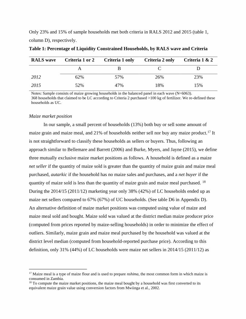
Only 23% and 15% of sample households met both criteria in RALS 2012 and 2015 (table 1,

column D), respectively.

Table 1: Percentage of Liquidity Constrained Households, by RALS wave and Criteria

RALS wave Criteria 1 or 2 Criteria 1 only Criteria 2 only Criteria 1 & 2

A B C D

2012 62% 57% 26% 23%

2015 52% 47% 18% 15%

Notes: Sample consists of maize growing households in the balanced panel in each wave (N=6063).

368 households that claimed to be LC according to Criteria 2 purchased >100 kg of fertilizer. We re-defined these

households as UC.

Maize market position

In our sample, a small percent of households (13%) both buy or sell some amount of

maize grain and maize meal, and 21% of households neither sell nor buy any maize product.17 It

is not straightforward to classify these households as sellers or buyers. Thus, following an

approach similar to Bellemare and Barrett (2006) and Burke, Myers, and Jayne (2015), we define

three mutually exclusive maize market positions as follows. A household is defined as a maize

net seller if the quantity of maize sold is greater than the quantity of maize grain and maize meal

purchased, autarkic if the household has no maize sales and purchases, and a net buyer if the

quantity of maize sold is less than the quantity of maize grain and maize meal purchased. 18

During the 2014/15 (2011/12) marketing year only 38% (42%) of LC households ended up as

maize net sellers compared to 67% (67%) of UC households. (See table D6 in Appendix D).

An alternative definition of maize market positions was computed using value of maize and

maize meal sold and bought. Maize sold was valued at the district median maize producer price

(computed from prices reported by maize-selling households) in order to minimize the effect of

outliers. Similarly, maize grain and maize meal purchased by the household was valued at the

district level median (computed from household-reported purchase price). According to this

definition, only 31% (44%) of LC households were maize net sellers in 2014/15 (2011/12) as

17 Maize meal is a type of maize flour and is used to prepare nshima, the most common form in which maize is

consumed in Zambia. 18 To compute the maize market positions, the maize meal bought by a household was first converted to its

equivalent maize grain value using conversion factors from Mwiinga et al., 2002.

compared to 56% (68%) for UC households (See table D7 in Appendix D). This value based

maize market position was used for conducting robustness check.

Maize marketing channels

Smallholder households in Zambia sell maize to a wide variety of buyers and may make

more than one transaction in a marketing year. For tractability, we focus on the largest maize

transaction made by each household and group maize marketing channels into four categories:

the FRA, small scale private traders, large scale private traders, and other households. 19

In 2014/15 (2011/12) marketing year, 48% (64%) of households chose to sell to FRA,

26% (17%) to small scale traders, 16% (10%) to large scale traders, and 11% (9%) to other

households. A smaller percentage of LC households sold to the FRA as compared to UC

households in both years (table D8 in Appendix D). Almost 90% of the households selling to the

FRA had to travel >1 km to make the maize sale. In contrast, 74% (64%), 33% (30%), and 87%

(85%) of the transactions made to small scale traders, large scale traders, and other households in

2011/12 (2014/15) were made at the farmgate, respectively (tables D9 and D10 in Appendix D).

The median farmgate price received from the FRA was 42% (24%) higher than the price

received from small scale traders in 2011/12 (2014/15) marketing year. The median price

received for sales to other households was also slightly higher (1% and 8% for 2011/12 and

2014/15 respectively) than that for small scale traders (tables D9 and D10 in Appendix D). This

is probably because maize sales to other households were spread more evenly over the maize

marketing season and thus the prices received from this channel would reflect, in part, the higher

maize prices that prevail later in the marketing season.20

Even though during our period of analysis, the price offered by the FRA was higher than

private market prices on average, there was considerable uncertainty related to when FRA would

start buying maize and when farmers would be paid. Almost 50% of farmers who sold to FRA

had to wait for at least two months to be paid. In contrast, more than 90% of those who sold to

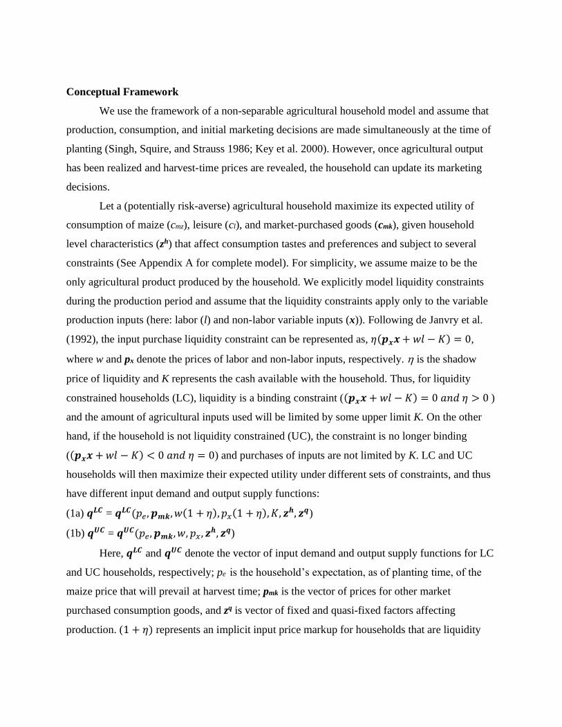
private traders or another household that year received payment at the time of the sale (Figure 1).

Further, even though harvesting begins in May, farmers typically have to wait until July or

19 A large majority of maize net sellers (87% in 2011/12 and 88% in 2014/15) had only one maize sale transaction in

the given marketing year. 20 Figure D2 in Appendix D shows that >50% of the largest maize transactions to other households occur in months

other than July, August, and September (the peak maize marketing months). This is in comparison to <10% for FRA

and <40% for small and large scale private traders.

August for the FRA to start buying maize. This, coupled with the delayed payments, would

likely lead to considerable discounting of the price offered by the FRA, especially for households

that may be in urgent need of cash. Another potential hurdle to selling to the FRA that

households may have to overcome is that, officially, 500 kg is the minimum amount of maize

that the FRA will buy from an individual or cooperative (Mason 2011). In contrast, the median

quantity of maize sold by LC households in our sample was only 50 kg; however, farmers can

overcome this hurdle by bulking their product with that of other farmers.

Figure 1: Number of months between sales transaction and payment to farmer for the

largest maize transaction

Estimation method

We break down the estimation method into several smaller and simpler steps.

Step 1

We first estimate the effect of being liquidity status and expected maize prices on maize

output using a linear switching regression. This approach allows the parameter estimates to differ

between LC and UC households, in line with the conceptual framework where LC and UC

households were found to be solving different optimizing problems and with similar previous

work (Feder et al. 1990; Foltz 2004; Winter-Nelson and Temu 2005).21 The availability of panel

data enables us to control for unobserved time-invariant household-level heterogeneity. Given

the non-linear-in-parameters nature of our estimators in the second step regression (discussed

below), we use a correlated random effects (CRE) approach (Mundlak 1978; Chamberlain 1984)

throughout the paper for consistency.22 23 In our analysis we operationalize CRE by including the

means of all time varying exogenous variables as additional regressors in our model. There may

be time-varying unobservables (such as an unreported access to productive resources from

family or friends) that are correlated with a household’s liquidity status as well as their maize

output leading to potential omitted variable bias. To overcome this problem, we use a two-step

control function endogenous switching CRE-pooled OLS (CRE-POLS) procedure as suggested

by Wooldridge (2015) and Murtazashvili and Wooldridge (2016). The two-step approach entails

estimating a first stage regression of liquidity status to obtain residuals that are used as an

additional regressor in the main equation. Details of the approach are discussed below. Equation

2 represents the main equation to be estimated:

(2) 𝑞𝑚𝑧,𝑖𝑡 = 𝐿𝐶𝑖𝑡 × 𝑿1𝑖𝑡𝜷1 + 𝑿1𝑖𝑡𝜷0 + 𝐿𝐶𝑖𝑡 × 𝑐𝑖 + 𝑐𝑖 + 𝐿𝐶𝑖𝑡 × 𝑣𝑡 + 𝑣𝑡 + 𝜏1𝐿𝐶𝑖𝑡 × 𝑢𝑖�̂� +

𝜏0𝑢𝑖�̂� + 𝜖𝑖𝑡

Here, 𝑞𝑚𝑧,𝑖𝑡 is the maize output of household i in agricultural year t, 𝐿𝐶𝑖𝑡 is an indicator variable

that equals 1 if the household was LC during the production period, and 0 if UC. 𝑿1𝑖𝑡 is the

vector of explanatory variables (including the vector of expected harvest-time maize prices (𝒑𝒆),

prices of agricultural inputs (𝒑𝒙 and w), household characteristics (𝒛𝒉), quasi-fixed factors (𝒛𝒒),

and rainfall and moisture shocks in the growing season). 𝑐𝑖 is the household-specific time

invariant unobserved heterogeneity, 𝑣𝑡 is the year fixed effect, 𝑢𝑖�̂� are the residuals from the first

stage regression of the liquidity status and 𝜖𝑖𝑡 is the idiosyncratic error specific to each household

21 We also estimate the equation using a 2SLS approach as a robustness check, as will be discussed later. 22 The fixed effect approach is not recommended for non-linear-in-parameters panel estimation when the number of

observations of the individual (N) tends to infinity but the number of time periods (T) is very small. Using a fixed

effects approach would require estimating parameters for each of the N units which are known be inconsistent. This

is known as the incidental parameters problem (Greene et al. 2002; Arellano and Hahn 2007). 23 Like a fixed-effects or (regular) random effects approach, a key assumption underlying the CRE approach is strict

exogeneity of the observed covariates conditional on the unobserved household-level time constant heterogeneity.

However, the CRE approach allows the observed covariates to be correlated with the unobserved heterogeneity like

the fixed effects approach, whereas the regular random effects approach assumes these two to be uncorrelated.

and time period. 𝜷1, 𝜷0 , 𝜏1, and 𝜏0 are the parameter values to be estimated.24 The estimates of

interest are the marginal effect of LC (𝐸(𝑞𝑚𝑧|𝐿𝐶 = 1) − 𝐸(𝑞𝑚𝑧|𝐿𝐶 = 0)) and marginal effect of

expected prices on maize output for LC and UC households (𝐸 [𝜕𝑞𝑚𝑧

𝜕𝒑𝒆| 𝐿𝐶 =

1] 𝑎𝑛𝑑 𝐸 [𝜕𝑞𝑚𝑧

𝜕𝒑𝒆| 𝐿𝐶 = 0] ).

Identification

The first stage regression that is used to control for potential endogeneity is estimated

using CRE-linear probability model of liquidity status (𝐿𝐶𝑖𝑡) on the full set of exogenous

variables (𝑿1𝑖𝑡) and an exclusion restriction (𝑧𝑖𝑡) and can be represented as follows:

(3) 𝐿𝐶𝑖𝑡 = 𝑿1𝑖𝑡𝜶1 + 𝛼2𝑧𝑖𝑡 + 𝑐𝑖 + 𝑣𝑡 + 𝑢𝑖𝑡

Identification hinges on the availability of a strong exclusion restriction – i.e., a variable that has

a strong statistically significant effect on the household’s selection into one of the two regimes,

yet which we can confidently assume is not correlated with the household’s maize output

through any channel other than its effect on liquidity. Our exclusion restriction is an indicator

variable that equals one if the village in which the household resides experienced a moisture

shock in the growing season prior to the planting season in which we measure liquidity

constraint. A moisture shock in year t-1 is expected to lead to poor crop output and thus a higher

chance of being liquidity constrained in the following year. We find that a moisture shock in year

t-1 is strongly partially correlated with being liquidity constrained in year t (F-statistic = 16.27,

p-value = 0.0001; see table E1 in Appendix E for the full results). Additionally, a moisture shock

in year t-1 should not affect maize output in year t through any channel other than its effect on

liquidity, particularly after controlling for rainfall conditions and the other covariates in year t, as

well as time-constraint unobserved heterogeneity via CRE. The validity of the instrument is

further discussed later in the article by conducting robustness checks.

Step 2

24 Failure to reject that 𝜏0=0 and 𝜏1=0 indicates that we fail to reject that liquidity status is exogenous to maize

output and can choose to use an exogenous version as the main analysis (we call this CRE-exogenous switching

regression). Alternatively, rejecting that at least one of the is equal to zero, would imply that liquidity status is

endogenous; the inclusion of the first stage residuals corrects for this endogeneity (conditional on the validity of the

exclusion restriction). We call this version the CRE-endogenous switching regression.

In the second step we estimate the effect of maize output on the household’s maize

market position using a CRE-ordered Probit approach. The respective probabilities of being a net

buyer and net seller of maize are given as follows:

(4) 𝑃𝑟(𝑀𝑖𝑡 = 1| 𝑞𝑚𝑧,𝑖𝑡 , 𝑿2𝑖𝑡 , 𝑐𝑖 , 𝑣𝑡) = Φ( 0 − (𝛿𝑞𝑚𝑧,𝑖𝑡 + 𝑿2𝑖𝑡𝜸 + 𝑐𝑖 + 𝑣𝑡))

(5) 𝑃𝑟(𝑀𝑖𝑡 = 3| 𝑞𝑚𝑧,𝑖𝑡 , 𝑿2𝑖𝑡 , 𝑐𝑖 , 𝑣𝑡) = Φ(𝛿𝑞𝑚𝑧,𝑖𝑡 + 𝑿2𝑖𝑡𝜸 + 𝑐𝑖 + 𝑣𝑡)

where, 𝑀𝑖𝑡 is the household’s maize market position (𝑀𝑖𝑡 =1 if net buyer, =2 if autarkic, and =3

if net seller); 𝑿2𝑖𝑡 is the vector of explanatory variables consisting of post-harvest farmgate price

of maize (pm); proxies for transaction costs or access to markets, and household characteristics. 𝛿

and 𝜸 are parameters to be estimated. The estimate of interest is the marginal effect of maize

output on market position (𝐸 ⌈𝜕Pr (𝑀=3)

𝜕𝑞𝑚𝑧⌉).

Step 3

The effect of maize output on the household’s maize marketing channel choice is estimated using

a CRE-Multinomial Logit (MNL) regression.25 The choice of marketing channel can be

represented as:

(6) 𝑃𝑟(𝑉𝑗𝑖𝑡 - 𝑉𝑘𝑖𝑡 > 0 | 𝑞𝑚𝑧,𝑖𝑡 , 𝑾𝑖𝑡 , 𝑐𝑖 , 𝑣𝑡) =

exp (𝜆𝑗𝑞𝑚𝑧,𝑖𝑡 + 𝑾𝑖𝑡 𝝅𝒋 + 𝑐𝑖 + 𝑣𝑡)

1 + ∑ exp(𝜆𝑗𝑞𝑚𝑧,𝑖𝑡 + 𝑾𝑖𝑡 𝝅𝒋 + 𝑐𝑖 + 𝑣𝑡)4𝑗=1

⁄

Here 𝑉𝑗𝑖𝑡- 𝑉𝑘𝑖𝑡 is the difference in utilities obtained from choosing channel j vs. channel k.

𝑞𝑚𝑧,𝑖𝑡 is as defined before and 𝑾𝑖𝑡 is a vector of control variables consisting of 𝑿2𝑖𝑡 (same as in

Step 2) and residuals from a selection equation described below. 𝜆𝑗 and 𝝅𝒋 are parameters

associated with marketing channel j. The estimate of interest to us is the marginal effect of maize

output on choice of marketing channel (𝐸 ⌈𝜕Pr (𝑉𝑗 − 𝑉𝑘>0)

𝜕𝑞𝑚𝑧⌉).

The CRE-MNL is estimated for the subset of maize net sellers only which can introduce

selection bias if the net selling maize growers are non-randomly different from other maize-

growing households in the full sample based on unobservable, time-varying characteristics. To

address this potential problem, we first estimate a CRE-Tobit selection equation for the net

maize quantity sold using the full sample, where net maize sales are zero for autarkic and net-

25 MNL is chosen over Multinomial Probit because the former is known to be computationally less cumbersome and

easier to interpret (Wooldridge 2010).

buying households. The generalized residuals from this Tobit regression are then used as an

additional regressor in the CRE-MNL to control for sample selection. The use of Tobit instead of

Probit as a selection equation allows us to solve the selection problem without the need of an

exclusion restriction. 26

Test of Hypothesis

The estimates from Step 1 and Step 2 are multiplied as shown in table 2 to test the

hypothesis 1 and 2. Similarly, the product of estimates from Step 1 and Step 3 are used to test the

hypothesis 3. Standard errors are computed by bootstrapping over 500 replications.

Table 2: Estimates to be Computed for Testing the Hypotheses

Results

Table 3 reports the Average Partial Effects (APEs) from the CRE-POLS switching

regressions for maize output by liquidity status for key variables of interest (See table E2 and E3

in Appendix E for full results). The residuals in the endogenous switching regression are not

statistically significant (at 10% level of significance); thus, we conclude that, controlling for the

observables and time invariant unobserved heterogeneity via CRE, liquidity status at planting

time is exogenous to maize output. In the subsequent discussion and computations, we focus on

26 Using a Probit selection equation without an exclusion restriction could lead to severe collinearity between the

generated residuals and explanatory variables. Identification in such a case relies on the nonlinearity of the inverse

mills ratio. In contrast, because the variation in the quantity of maize sold among net sellers is leveraged in the Tobit

selection equation, the Tobit residuals have separate variation from the explanatory variables of the main regression

(here, CRE-MNL), thus alleviating concerns of collinearity and providing a way to control for sample selection bias

even in the absence of an exclusion restriction. (See Wooldridge (2010) for details).

Hypothesis Statement Estimates

1 LC maize-producing households are

less likely to become maize net sellers

𝐸[(𝑞𝑚𝑧|𝐿𝐶 = 1) − (𝑞𝑚𝑧|𝐿𝐶 = 0)] *

𝐸 ⌈𝜕Pr (𝑀 =3))

𝜕𝑞𝑚𝑧⌉ < 0

2

A LC household’s probability to sell

maize will be less responsive to

changes in expected prices

𝐸 [𝜕𝑞𝑚𝑧

𝜕𝒑𝒆| 𝐿𝐶 = 1] * 𝐸 ⌈

𝜕Pr (𝑀 =3))

𝜕𝑞𝑚𝑧⌉ <

𝐸 [𝜕𝑞𝑚𝑧

𝜕𝒑𝒆| 𝐿𝐶 = 0] * 𝐸 ⌈

𝜕Pr (𝑀 =3))

𝜕𝑞𝑚𝑧⌉

3 Net seller LC households are less

likely to sell to FRA

𝐸[(𝑞𝑚𝑧|𝐿𝐶 = 1) − (𝑞𝑚𝑧|𝐿𝐶 = 0)] ∗

𝐸 ⌈𝜕Pr (𝑉𝐹𝑅𝐴 − 𝑉𝑘>0)

𝜕𝑞𝑚𝑧⌉ < 0

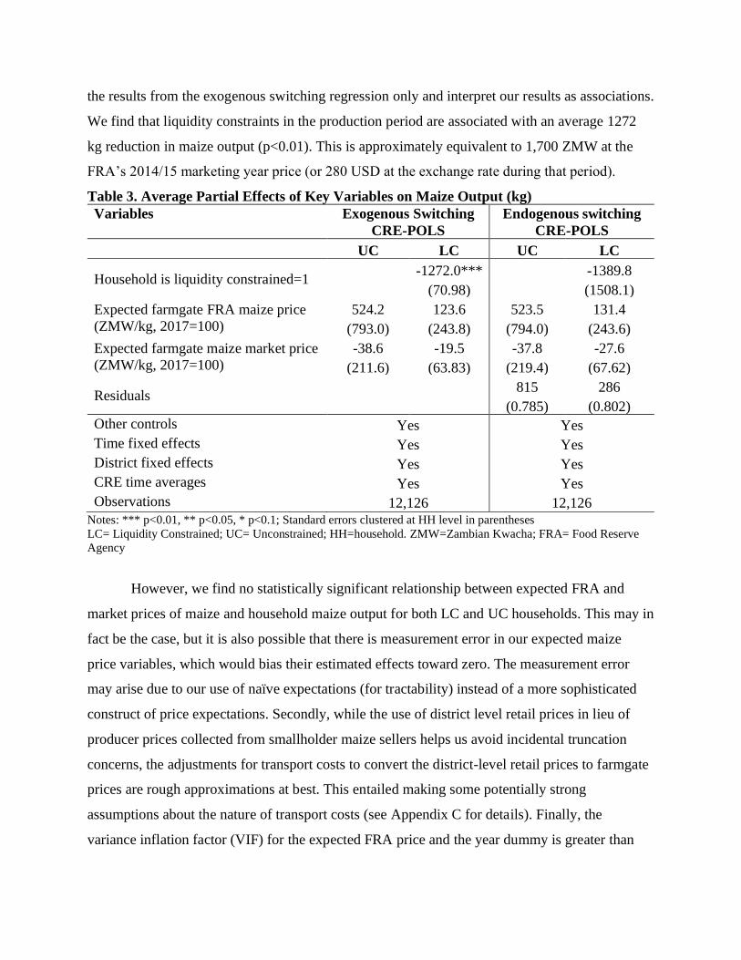
the results from the exogenous switching regression only and interpret our results as associations.

We find that liquidity constraints in the production period are associated with an average 1272

kg reduction in maize output (p<0.01). This is approximately equivalent to 1,700 ZMW at the

FRA’s 2014/15 marketing year price (or 280 USD at the exchange rate during that period).

Table 3. Average Partial Effects of Key Variables on Maize Output (kg)

Variables Exogenous Switching

CRE-POLS

Endogenous switching

CRE-POLS

UC LC UC LC

Household is liquidity constrained=1 -1272.0*** -1389.8

(70.98) (1508.1)

Expected farmgate FRA maize price

(ZMW/kg, 2017=100)

524.2 123.6 523.5 131.4

(793.0) (243.8) (794.0) (243.6)

Expected farmgate maize market price

(ZMW/kg, 2017=100)

-38.6 -19.5 -37.8 -27.6

(211.6) (63.83) (219.4) (67.62)

Residuals 815 286

(0.785) (0.802)

Other controls Yes Yes

Time fixed effects Yes Yes

District fixed effects Yes Yes

CRE time averages Yes Yes

Observations 12,126 12,126 Notes: *** p<0.01, ** p<0.05, * p<0.1; Standard errors clustered at HH level in parentheses

LC= Liquidity Constrained; UC= Unconstrained; HH=household. ZMW=Zambian Kwacha; FRA= Food Reserve

Agency

However, we find no statistically significant relationship between expected FRA and

market prices of maize and household maize output for both LC and UC households. This may in

fact be the case, but it is also possible that there is measurement error in our expected maize

price variables, which would bias their estimated effects toward zero. The measurement error

may arise due to our use of naïve expectations (for tractability) instead of a more sophisticated

construct of price expectations. Secondly, while the use of district level retail prices in lieu of

producer prices collected from smallholder maize sellers helps us avoid incidental truncation

concerns, the adjustments for transport costs to convert the district-level retail prices to farmgate

prices are rough approximations at best. This entailed making some potentially strong

assumptions about the nature of transport costs (see Appendix C for details). Finally, the

variance inflation factor (VIF) for the expected FRA price and the year dummy is greater than

10, signalling a multicollinearity issue.27 The correlation coefficient between these two variables

is also very high (0.90). This is expected because there is relatively little variation in FRA

farmgate prices within a year due to the pan-territorial nature of FRA depot-level price. We

therefore interpret with caution the estimated effects of the expected maize prices on maize

output.

A comparison of APEs of landholding size of LC and UC households reveals that UC

households are able to produce, on average, 430 kg more maize from an additional hectare of

land as compared to LC households (table E4 in Appendix E). This is what we would expect if

LC households are constrained in their ability to invest in sufficient inorganic fertilizer or

improved seed to use land productively. It is also plausible that the effect of liquidity constraints

are heterogenous across different landholding categories. This is especially relevant given the

recent rise in the prominence of medium scale farmers (i.e., those farming 5+ hectares of land) in

Zambia and other land abundant countries in SSA. These farmers are found to have better access

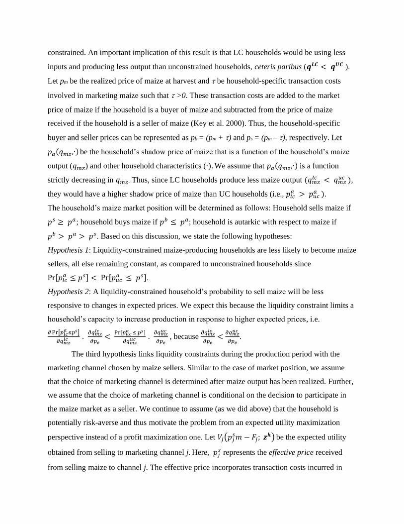
to resources and political leverage to influence agricultural policy (Jayne et al. 2019). Figure 2

shows that LC households across all landholding sizes produce less maize output than UC

households, and more importantly, the difference in maize output between LC and UC

households goes on increasing as the landholding size increases. A caveat worth noting here is

that almost 90% of LC households in our sample owned 5 hectares or less of land compared to

75% of UC households.

We further use the CRE-POLS switching approach to interrogate the premise that the

difference in maize output between LC and UC households is at least partly due to LC

households’ relatively lower capacity to invest in maize productivity-enhancing inputs – e.g.,

inorganic fertilizer and improved seed.28 The results of these regressions (table E5 in Appendix

E) suggest that being liquidity constrained is associated with a 113 kg/ha reduction in the rate of

fertilizer application to maize and a 19 percentage point reduction in the probability of growing

an improved maize variety, on average (p<0.01). These numbers represent a 55% and 25%

reduction in use of fertilizer and improved seed, respectively. They further emphasize the losses

incurred by the inability to use land productively through investment in inorganic fertilizer and

improved seed.

27 The VIF for all other variables was within the acceptable range (<=10). 28 Improved seed refers to both hybrids and improved open pollinated varieties.

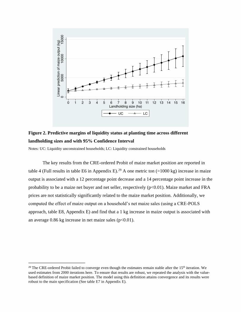
Figure 2. Predictive margins of liquidity status at planting time across different

landholding sizes and with 95% Confidence Interval

Notes: UC: Liquidity unconstrained households; LC: Liquidity constrained households

The key results from the CRE-ordered Probit of maize market position are reported in

table 4 (Full results in table E6 in Appendix E).29 A one metric ton (=1000 kg) increase in maize

output is associated with a 12 percentage point decrease and a 14 percentage point increase in the

probability to be a maize net buyer and net seller, respectively (p<0.01). Maize market and FRA

prices are not statistically significantly related to the maize market position. Additionally, we

computed the effect of maize output on a household’s net maize sales (using a CRE-POLS

approach, table E8, Appendix E) and find that a 1 kg increase in maize output is associated with

an average 0.86 kg increase in net maize sales (p<0.01).

29 The CRE-ordered Probit failed to converge even though the estimates remain stable after the 15th iteration. We

used estimates from 2000 iterations here. To ensure that results are robust, we repeated the analysis with the value-

based definition of maize market position. The model using this definition attains convergence and its results were

robust to the main specification (See table E7 in Appendix E).

Table 4. Average Partial Effects of Key Variables on the Maize Market Position (CRE-

ordered Probit)

Variables Net-buyer Autarkic Net-seller

Quantity of maize produced, kg -0.00012*** -0.000020*** 0.00014***

(0.000016) (0.0000015) (0.000016)

Farmgate maize price

(ZMW/kg, 2017=100)

-0.0021 -0.00036 0.0025

(0.012) (0.0020) (0.014)

Farmgate FRA maize price

(ZMW/kg, 2017=100)

-0.061 -0.010 0.071

(0.106) (0.018) (0.124)

Other controls Yes

Time fixed effects Yes

District fixed effects Yes

CRE time averages Yes

Observations 12126 Notes: *** p<0.01, ** p<0.05, * p<0.1; Standard errors clustered at HH level in parentheses

LC= Liquidity Constrained; UC= Unconstrained; HH=household. ZMW=Zambian Kwacha; FRA= Food Reserve

Agency

Table 5 summarizes key results of the CRE-MNL for net selling households’ choice of

maize marketing channel for the largest transaction of maize (See tables E9 and E10 in Appendix

E for the first-stage CRE-Tobit for the quantity of maize sold and the full CRE-MNL results,

respectively). An additional unit of maize produced does not have any statistically significant

relation with choosing to sell to small scale traders. However, a one metric ton increase in maize

produced is associated with a 4 percentage point increase in probability to sell to FRA, a 1.2

percentage point increase in probability to sell to large scale traders, and a 5.4 percentage point

decrease in probability to sell to other households (p<0.01). These results support our exposition

that households that produce a larger maize surplus would be more likely to sell to marketing

channels that entail larger fixed costs (such as uncertainty and delay for FRA, negotiation and

search costs for large scale sellers, and transport for both).

The estimates computed above are used to test the hypotheses as detailed in table 2 and

the results are summarised in table 6. In support of hypothesis 1, LC households are found to be

18 percentage points less likely to be a net seller of maize due the inability to produce a

marketable surplus (p<0.05). We do not find evidence of statistically significant effect of

expected maize price on households’ probability of being net sellers for either LC or UC

households. However, as discussed earlier, due to caveats about measurement error in expected

prices we are unable to make a confident conclusion about hypothesis 2. Lastly, consistent with

hypothesis 3, being liquidity constrained is found to be associated with 5 percentage point

reduction in the probability of selling to FRA. LC households are also found to be 2 percentage

points less likely to sell to large scale traders but 7 percentage points more likely to sell to other

households (p<0.05). There is no statistically significant relationship between being liquidity

constrained and selling to small scale traders.

Table 5. Average Partial Effects of Maize Output on Choice of Marketing Channel made

for the Largest Transaction of Maize by Net Seller Households (CRE-Multinomial Logit)

Variables Average Partial Effects

Small scale

traders FRA

Large scale

traders

Other

households

Quantity of maize produced,

kg

0.0000030 0.000039*** 0.000012*** -0.000054***

(0.0000081) (0.0000089) (0.0000036) (0.000013)

Residuals from CRE-Tobit

selection equation§ Yes

Time fixed effects Yes

Province fixed effects# Yes

CRE time averages Yes

Observations 7108 Notes: *** p<0.01, ** p<0.05, * p<0.1; standard errors are clustered at household level and bootstrapped with 500

replications to account for the generated regressor (CRE-Tobit residuals). §The CRE-Tobit residuals are significant

at 1% level of significance, implying that the sample of net sellers was non-random and our estimates would have

been biased if we had not corrected them through inclusion of the residuals; #Province fixed effects were used in

place of district fixed effects because the model failed to converge when using the latter.

Finally, to alleviate concerns about the hypothetical bias in the definition of liquidity

status, we re-conduct the analysis using the alternate definition of liquidity (criteria 2 only).

Results from the analysis are presented in tables E11 and E12 in Appendix E. We find that LC

households produce on average 1562 kg less maize as compared to UC households, and thus are

22 percentage points less likely to be net sellers of maize (p<0.01). LC households that are net

sellers are 6 percentage points less likely to sell to FRA (p<0.01). These estimates are consistent

with those obtained from the main specification.

Table 6. Test of Hypotheses

Hypothesis Effect of interest APE

1

Liquidity constraint on the probability of being a net buyer 0.15**

(0.077)

Liquidity constraint on the probability of being a net seller -0.18**

(0.088)

2

Expected FRA price on probability of being a net seller for LC

HH

0.017

(0.051)

Expected FRA price on probability of being a net seller for UC

HH

-0.003

(0.013)

Market price on probability of being a net seller for LC HH 0.074

(0.169)

Market price on probability of being a net seller for UC HH -0.005

(0.031)

3

Liquidity constraint on the probability of selling to a small scale

trader

-0.004

(0.007)

Liquidity constraint on the probability of selling to FRA -0.049**

(0.024)

Liquidity constraint on the probability of selling to a large scale

trader

-0.015**

(0.007)

Liquidity constraint on the probability of selling to other

households

0.068**

(0.031) Notes: *** p<0.01, ** p<0.05, * p<0.1; Standard errors in parentheses are based on 500 bootstrap replications

APE= Average partial Effect; LC= Liquidity Constrained; UC= Unconstrained; HH=Household; FRA= Food

Reserve Agency

Robustness checks

We discuss some of the limitations of this study and the additional analyses conducted

(wherever possible) to address them.

Validity of the instrument variable

The lagged moisture shock variable we use as an instrument may not be valid if there are

channels apart from its effect on liquidity constraint that can influence maize output. For

example, a moisture shock in period t-1 could affect maize output through a change in soil

quality that persists into period t. We do not have a way to test this but do not expect this be a

serious concern. A persistent change in soil quality is only likely if the dry spell is very severe. In

such a case, soil nitrogen becomes unavailable to the plant in t-1 and leads to a carry-over of this

nitrogen into the next season, which would increase the maize yield in period t (S. Snapp,

personal communication, April 2, 2020). Thus, in the rare case that the instrument affects the

maize output through a change in soil quality, our estimates of the impact of liquidity would be

biased upwards (less negative effect of LC) and can still be considered as a conservative lower

limit to the true effect.

A second concern is related to potential serial correlation in the moisture shock variables.

If some geographical locations are more prone to experiencing dry spells over several years, a

moisture shock in period t-1 would also be linked to weather conditions in period t, and thus to

maize output. We alleviate some of this concern by including information on long term average

growing season moisture shock and rainfall in our models. Our use of CRE to control for time-

constant unobserved heterogeneity should also alleviate some of these concerns. In addition, we

run a falsification test by including a lead of the moisture shock variable (i.e., the moisture shock

in period t+1) in the first stage CRE-POLS for liquidity status and the CRE-switching POLS for

maize output. We test the null hypotheses that maize output and liquidity status are not correlated

with moisture shocks in the next time period through any serial correlation in the moisture shock

variable. We fail to reject this null for both liquidity status and maize output which further

supports the validity of the instrument (Full results in table E13 in Appendix E).

Two-stage least squares as an alternative to switching regression

The maize output equation is re-analyzed with a using CRE-two stage least squares

(2SLS) approach as an alternative to the endogenous switching CRE-POLS of maize output to

ensure robustness of our results. Unfortunately, we are unable to generate the effect of expected

maize prices for LC and UC households separately due to lack of sufficiently strong IVs of the

interaction terms of liquidity status and expected prices. The results (recorded in table E13 in

Appendix E) show that LC households produce 2698 kg less maize, on average, than UC

households (p<0.1). The test of endogeneity of liquidity status in the 2SLS estimation fails to

reject the null of exogeneity. Both these results are consistent with our main results.

Sensitivity analysis using different measures of prices

We use two alternative measures of market prices to check if our results are sensitive to

the measure of maize market price used in the main analysis. The first measure is a moving

average of monthly maize retail prices over the entire peak maize marketing season (May-

October). The second is a similar measure computed for the months of July, August, and

September only. Using these alternative measures of prices, however, does not change the

analysis in any significant manner (Full results in tables E14 and E15, Appendix E). Both maize

output and maize market position remain unresponsive to expected prices and realized prices,

respectively.

Conclusions and policy implications

In this article we study the effect of liquidity constraints during production period on

Zambian maize growing smallholders’ market participation in maize markets. We show

empirically that liquidity constrained households are not able to invest adequately in

productivity-enhancing inputs (e.g., inorganic fertilizer and improved maize seed), limiting their

capacity to produce a marketable surplus, thereby decreasing their probability of being a net

seller. These results are consistent with those of Alene et al. (2007), Boughton et al. (2007), and

Mather et al. (2013), which found that insufficient access to public and private assets can limit a

smallholder household from producing a marketable surplus of a food crop and thus reduce their

participation in food grain output markets. They are also in alignment to Fink, Jack, and Masiye

(2020) who show that a small credit intervention in the lean season in rural Zambia leads to

significant improvements in agricultural production by releasing family labor from non-farm

piecework to devote more time on farm work.

We hypothesized but did not find strong evidence that liquidity constrained households

are less responsive to an increase in expected maize prices. We suspect measurement error in the

price variables and issues of multicollinearity could be partially responsible for the lack of strong

evidence. Finally, we find evidence that liquidity constraints are associated with the marketing

channel chosen by the household for largest maize sale. Since liquidity constrained households

produce lower marketable surplus, they are less likely to overcome the high fixed costs

associated with accessing some channels. Specifically, in the case of maize markets in Zambia,

liquidity constrained net seller households were found to be less likely to sell to the parastatal

marketing board, FRA, as compared to small scale traders and other households. Overall, our

results show that production bottlenecks, such as liquidity constraints at the time of planting, can

limit a household’s capacity to benefit from remunerative market and price policies. These

results support the view that price policies may have limited effects on smallholders’ food

production and marketing responses if they lack access to the productive assets and inputs

needed to expand production (Barrett 2008). This can exacerbate the benefits of agricultural

market policies being disproportionately captured by wealthier farmers as has indeed been

reported in the case of Zambia (Jayne et al. 2011; Fung et al. 2020). The results also have

implications for a land abundant country like Zambia where much of the increase in maize

production has been a result of increase in crop acreage and not through an increase in

productivity (Burke et al. 2010). In recent years, the FRA has subdued its activities as a major

buyer of maize in Zambia and has shifted attention towards provision of food relief to vulnerable

population. There has also been evidence of better participation by private sector players in

maize output markets (Mulenga et al. 2019). This is a welcome shift in light of the results of this

article and the recent threat to the food security of Zambia due to droughts in the 2017/18 and

2018/19 agricultural season. The resources of the government spent on large scale interventions

by the FRA in maize markets, could be better spent in improving the productivity and resilience

of smallholder farmers.

References

Alene, A.D., V. Manyong, G. Omanya, H. Mignouna, M. Bokanga, and G. Odhiambo. 2008.

“Smallholder Market Participation under Transactions Costs: Maize Supply and Fertilizer

Demand in Kenya.” Food Policy 33:318–328.

Arellano, M., and Hahn, J. 2007. “Understanding Bias in Nonlinear Panel Models: Some recent

developments”. Econometric Society Monographs, 43, 381.

Barrett, C.B. 2008. “Smallholder Market Participation: Concepts and Evidence from Eastern

and Southern Africa.” Food Policy 33:299–317.

Bellemare, M. F., and Barrett, C. B. 2006. “An Ordered Tobit Model of Market Participation:

Evidence from Kenya and Ethiopia”. American Journal of Agricultural Economics, 88(2),

324-337.

Binswanger, H. P., and Braun, J. 1991. “Technological Change and Commercialization in

Agriculture: The Effect on the Poor” The World Bank Research Observer 6(1):57-80.

Boughton, D., D. Mather, C.B. Barrett, R.S. Benfica, D. Abdula, D. Tschirley, and B. Cunguara.

2007. “Market Participation by Rural Households in a Low-Income Country: An Asset

Based Approach Applied to Mozambique.” Faith and economics 50:64–101.

Burke, W.J., T.S. Jayne, and A. Chapoto. 2010. “Factors Contributing to Zambia’s 2010 Maize

Bumper Harvest”. Working Paper no. 48, Food Security Research Project, Michigan State

University, East Lansing, MI.

Burke, W.J., Jayne, T.S., and Sitko, N. 2012. “Can the FISP more Effectively Achieve Food

Production and Poverty Reduction Goals?” Policy Synthesis No.51- Food Security

Research Project, Zambia, Michigan State University, East Lansing.

Burke, M., Bergquist, L. F., and Miguel, E. 2019. “Sell Low and Buy High: Arbitrage and Local

Price Effects in Kenyan markets”. The Quarterly Journal of Economics, 134(2), 785-842.

Burke, W. J., Myers, R. J., and Jayne, T. S. 2015. A Triple-Hurdle Model of Production and

Market Participation in Kenya's dairy market. American Journal of Agricultural

Economics, 97(4), 1227-1246.

Cadot, O., M. Olarreaga, and L. Dutoit. 2006. “How Costly is it for Poor Farmers to Lift

themselves out of Poverty?” World Bank Policy Research Working Paper 3661, World Bank,

Washington, D.C.

Carter, M. R., and Lybbert, T. J. 2012. “Consumption Versus Asset Smoothing: Testing the

Implications of Poverty Trap Theory in Burkina Faso”. Journal of Development

Economics, 99(2), 255-264.

Chamberlain, G. 1984. “Panel data.” Handbook of Econometrics 2:1247–1318.

Chamberlin, J. and T.S. Jayne. 2013. "Unpacking the Meaning of ‘Market Access’: Evidence

from Rural Kenya," World Development, 41(C): 245-264.

Chapoto, A., O. Zulu-Mbata, B.D. Hoffman, C. Kabaghe, N. Sitko, A. Kuteya, and B. Zulu.

2015. “The Politics of Maize in Zambia: Who holds the keys to change the status quo.” Working

paper No. 99, Indaba Agricultural Policy Research Institute, IAPRI, Lusaka,

Zambia.

Central Statistical Office (CSO). 2012. RALS 2012: “Instruction Manual for Listing, Sample

Selection, and Largest Maize Field Data Collection”, Lusaka, Zambia.

Central Statistical Office (CSO). 2018. Administrative data obtained from the Central Statistical

Office, Lusaka, Zambia.

de Janvry, A., M. Fafchamps, and E. Sadoulet. 1991. “Peasant Household Behavior with Missing

Markets: Some Paradoxes Explain.” Economic Journal 101:1400–1417.

de Janvry, A., E. Sadoulet, M. Fafchamps, and M. Raki. 1992. “Structural Adjustment and the

Peasantry in Morocco: A Computable Household Model.” European Review of

Agricultural Economics 19:427–453.

Dercon, S., and Christiaensen, L. 2011. “Consumption Risk, Technology Adoption and Poverty

Traps: Evidence from Ethiopia”. Journal of Development Economics, 96(2), 159-173.

Dillon, B. 2020. “Selling Crops Early to Pay for School: A Large-scale Natural Experiment in

Malawi”. Journal of Human Resources, 0617-8899R1.

Dillon, B., and Dambro, C. 2017. “How Competitive are Crop Markets in Sub-Saharan Africa?”

American Journal of Agricultural Economics, 99(5), 1344-1361.

Duflo, E., M. Kremer, and J. Robinson. 2011. “Nudging Farmers to Use Fertilizer: Theory and

Experimental Evidence from Kenya”. American Economic Review 101(6):2350-90.

Fafchamps, M., and R.V. Hill. 2005. “Selling at the Farmgate or Traveling to Market.” American

Journal of Agricultural Economics 87:717–734.

FAO. 2007. “Compendium of Agricultural - Environmental Indicators (1989-91 to 2000): Annex

2 Definitions”. Rome: Food and Agricultural Organization.

Feder, G., L.J. Lau, J.Y. Lin, and X. Luo. 1990. “The Relationship Between Credit and

Productivity in Chinese Agriculture: A Microeconomic Model of Disequilibrium.”

American Journal of Agricultural Economics 72:1151–1157.

Fink, G., B. K. Jack and F. Masiye. 2020. "Seasonal Liquidity, Rural Labor Markets, and

Agricultural Production." American Economic Review, 110(11):3351-92.

Foltz, J.D. 2004. “Credit Market Access and Profitability in Tunisian Agriculture.” Agricultural

Economics 30:229–240.

Food Reserve Agency (FRA). n.d. Administrative data obtained from FRA, Lusaka, Zambia.

Fung, W., L.S.O, Liverpool-Tasie, N. Mason and R.U. Oyelere. “Do Crop Purchase Programs

Improve Smallholder Welfare? The case of Zambia’s Food Reserve Agency”. Agricultural

Economics 51:519–533.

Goetz, S.J. 1992. “A Selectivity Model of Household Food Marketing Behavior in Sub-Saharan

Africa.” American Journal of Agricultural Economics 74:444–452.

Greene, W., Han, C., and Schmidt, P. 2002. "The Bias of the Fixed Effects Estimator in

Nonlinear Models”. Unpublished Manuscript, Stern School of Business, NYU, 29.

Heltberg, R., and F. Tarp. 2002. “Agricultural Supply Response and Poverty in Mozambique.”

Food Policy 27:103–124.

Jayne, T.S., N.M. Mason, W.J. Burke, A.M. Shipekesa, A. Chapoto, and C. Kabaghe. 2011.

“Mountains of maize, persistent poverty.” Working paper No. 48, Indaba Agricultural

Policy Research Institute, IAPRI, Lusaka, Zambia.

Jayne, T.S., M. Muyanga, A. Wineman, H. Ghebru, C. Stevens, M. Stickler, A. Chapoto, W.

Anseeuw, D. Van der Westhuizen, and D. Nyange. 2019 "Are Medium‐Scale Farms

Driving Agricultural Transformation in Sub‐Saharan Africa?" Agricultural Economics 50:

75-95.

Key, N., E. Sadoulet, and A.D. Janvry. 2000. “Transactions Costs and Agricultural Household

Supply Response.” American Journal of Agricultural Economics 82:245–259.

Kusunose, Y., Mason-Wardell, N., and Tembo, S. 2020. The Role of Liquidity in Preventing

Dis-investment in Crop Inputs: Evidence from Zambia. Journal of African Economies

29(4):375-396.

Kuteya, A., Chinmaya, L., and Malata, V.C. 2018. “Review of E-FISP performance during

2017/2018 agricultural season” Monitoring report 2018, Indaba Agricultural Policy

Research Institute (IAPRI), Lusaka, Zambia.

Maidment, R.I., D. Grimes, R.P. Allan, E. Tarnavsky, M. Stringer, T. Hewison, R. Roebeling,

and E. Black. 2014. “The 30 Year TAMSAT African Rainfall Climatology and Time Series

(TARCAT) Data Set”. Journal of Geophysical Research: Atmospheres 119.18: 610-619.

Mason, N.M. 2011. “Marketing Boards, Fertilizer Subsidies, Prices, and Smallholder Behavior:

Modeling and Policy Implications for Zambia”. PhD Dissertation, Michigan State

University, East Lansing, Michigan.

Mason, N.M., and R.J. Myers. 2013. “The Effects of the Food Reserve Agency on Maize Market

Prices in Zambia.” Agricultural Economics 44:203–216.

Mason, N. M., Jayne, T. S., and Mofya-Mukuka, R. 2013. “A Review of Zambia’s agricultural

input subsidy programs: Targeting, impacts, and the way forward” Working paper no. 71,

Indaba Agricultural Policy Research Institute (IAPRI), Lusaka, Zambia.

Mason, N.M., T.S. Jayne, and R.J. Myers. 2015. “Smallholder Supply Response to Marketing

Board Activities in a Dual Channel Marketing System: The case of Zambia.” Journal of

Agricultural Economics 66:36–65.

Mather, D., D. Boughton, and T. Jayne. 2013. “Explaining Smallholder Maize Marketing in

Southern and Eastern Africa: The Roles of Market Access, Technology and Household

Resource Endowments.” Food Policy 43:248–266.

Muamba, F.M. 2011. “Selling at the Farmgate or Traveling to the Market: A Conditional Farm-

Level Model.” The Journal of Developing Areas 44(2): 95–107.

Mulenga, B.P., Banda, A., Chapoto, A., and Chisanga, B. 2019. “Zambian Maize Outlook and

Regional Analysis, 2019/20”. Indaba Agricultural Policy Research Institute (IAPRI),

Lusaka: Zambia.

Mundlak, Y. 1978. “On the Pooling of Time series and Cross Section Data.” Econometrica

46(1):69–85.

Murtazashvili, I. and Wooldridge, J.M. 2016. “A Control Function Approach to Estimating

Switching Regression Models with Endogenous Explanatory Variables and Endogenous

Switching”. Journal of Econometrics, 190:252-266.

Mwiinga, B., J.J. Nijhoff, T.S. Jayne, G. Tembo, and J.D. Shaffer. 2002. “The Role of Mugaiwa

in Promoting Household Food Security: Why it Matters Who Gets Access to Government

Maize Imports?” Policy Synthesis-No. 5, Food Security Research Project- Zambia. East

Lansing, Michigan.

Negi, D.S., P.S. Birthal, D. Roy, and M.T. Khan. 2018. “Farmers a Choice of Market Channels

and Producer Prices in India: Role of Transportation and Communication Networks.” Food

Policy 81:106–121.

Pingali, P., Y. Khwaja, and M. Meijer. 2005. “Commercializing Small Farms: Reducing

Transaction Cost”. ESA Working Paper No. 05-08, Food and Agriculture organization

(FAO), United Nations.

Renkow, M., D.G. Hallstrom, and D.D. Karanja. 2004. “Rural Infrastructure, Transactions Costs

and Market Participation in Kenya.” Journal of Development Economics 73:349–367.

Sadoulet, E., and de Janvry, A. 1995. Quantitative development policy analysis (Vol. 5).

Baltimore: Johns Hopkins University Press

Shilpi, F., and D. Umali-Deininger. 2008. “Market Facilities and Agricultural Marketing:

Evidence from Tamil Nadu, India.” Agricultural Economics 39:281–294.

Singh, I., L. Squire, and J. Strauss. 1986. “A Survey of Agricultural Household Models: Recent

Findings and Policy Implications.” The World Bank Economic Review 1:149–179.

Sitko, N.J., and T. Jayne. 2014. “Exploitative Briefcase Businessmen, Parasites, and other Myths

and Legends: Assembly Traders and the Performance of Maize Markets in Eastern and

Southern Africa.” World Development 54:56–67.

Snapp S. 2020, April 2. Communication through email with A. Melkani.

Snyder, J., T.S. Jayne, N. Mason, P. Samboko. 2019. “Agricultural Productivity and Rural

Household Incomes: Micro-level Evidence from Zambia”. Feed the Future Innovation Lab

for Food Security Policy Research Paper 151. East Lansing, Michigan.

Stephens, E.C., and C.B. Barrett. 2011. “Incomplete Credit Markets and Commodity Marketing

Behaviour.” Journal of Agricultural Economics 62:1–24.

Takeshima, H., and A. Winter-Nelson. 2012. “Sales Location among Semi-Subsistence Cassava

Farmers in Benin: A Heteroskedastic Double Selection Model.” Agricultural Economics

43:655–670.

Tarnavsky, E., D. Grimes, R. Maidment, E. Black, R.P. Allan, M. Stringer, R. Chadwick, and F.

Kayitakire. 2014. “Extension of the TAMSAT Satellite-Based Rainfall Monitoring over

Africa and from 1983 to Present”. Journal of Applied Meteorology and Climatology 53.12:

2805-2822.

Timmer, C.P. 1988. “The Agricultural Transformation” In H. B. Chenery, T. N. Srinivasan, T.P.

Schultz, J.R. Behrman, J. R., J. Strauss, D. Rodrik, and M.R. Rosenzweig (Eds.) Handbook

of development economics (Vol. 4). Elsevier, pp: 275–331.

von Braun, J., and E. T. Kennedy .1994. “Agricultural Commercialization, Economic

Development, and Nutrition”. Published for the International Food Policy Research

Institute (IFPRI), Washington D.C.

von Braun, J. 1995. “Agricultural Commercialization: Impacts on Income and Nutrition and

Implications for Policy” Food Policy 20(3):187-202.

Winter-Nelson, A., and A.A. Temu. 2005. “Liquidity Constraints, Access to Credit and pro-Poor

Growth in Rural Tanzania.” Journal of International Development 17:867–882.

Wooldridge, J. M. 2010. Econometric Analysis of Cross Section and Panel Data. MIT Press.

Wooldridge, J.M. 2015. “Control Function Methods in Applied Econometrics.” Journal of

Human Resources 50:420–445.

World Bank. 2019a. World Development Indicators: Employment in Agriculture (% of total

employment). [Datafile]. Retrieved from: https://databank.worldbank.org/source/world-

development-indicators

World Bank. 2019b. World Development Indicators: Consumer Price Index. [Datafile].Retrieved

from: https://databank.worldbank.org/indicator/FP.CPI.TOTL.ZG/1ff4a498/Popular-

Indicators

Zanello, G., C.S. Srinivasan, and B. Shankar. 2014. “Transaction Costs, Information

Technologies, and the Choice of Marketplace among Farmers in Northern Ghana.” The

Journal of Development Studies 50:1226–1239.

Supplementary Material

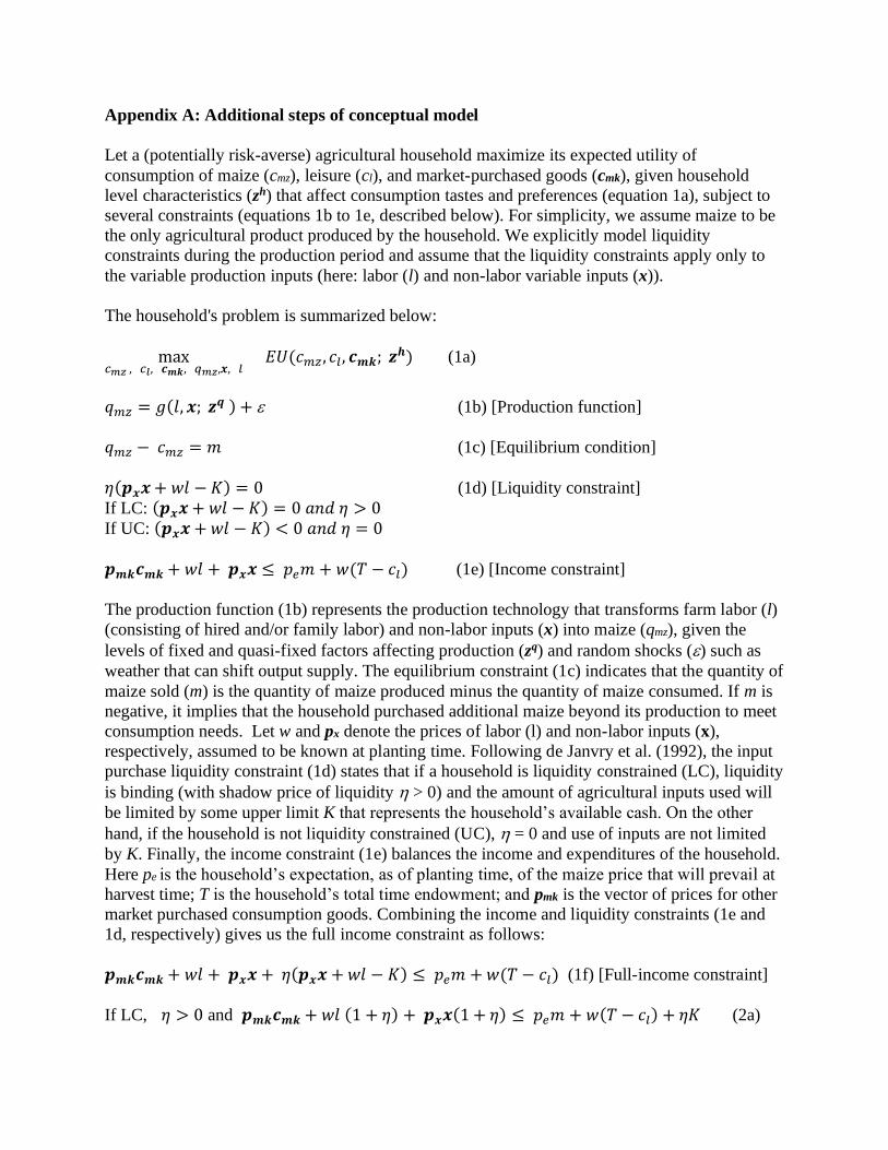
Appendix A: Additional steps of conceptual model

Let a (potentially risk-averse) agricultural household maximize its expected utility of

consumption of maize (cmz), leisure (cl), and market-purchased goods (cmk), given household

level characteristics (zh) that affect consumption tastes and preferences (equation 1a), subject to

several constraints (equations 1b to 1e, described below). For simplicity, we assume maize to be

the only agricultural product produced by the household. We explicitly model liquidity

constraints during the production period and assume that the liquidity constraints apply only to

the variable production inputs (here: labor (l) and non-labor variable inputs (x)).

The household's problem is summarized below:

max𝑐𝑚𝑧 , 𝑐𝑙, 𝒄𝒎𝒌, 𝑞𝑚𝑧,𝒙, 𝑙

𝐸𝑈(𝑐𝑚𝑧 , 𝑐𝑙 , 𝒄𝒎𝒌; 𝒛𝒉) (1a)

𝑞𝑚𝑧 = 𝑔(𝑙, 𝒙; 𝒛𝒒 ) + (1b) [Production function]

𝑞𝑚𝑧 − 𝑐𝑚𝑧 = 𝑚 (1c) [Equilibrium condition]

𝜂(𝒑𝒙𝒙 + 𝑤𝑙 − 𝐾) = 0 (1d) [Liquidity constraint]

If LC: (𝒑𝒙𝒙 + 𝑤𝑙 − 𝐾) = 0 𝑎𝑛𝑑 𝜂 > 0

If UC: (𝒑𝒙𝒙 + 𝑤𝑙 − 𝐾) < 0 𝑎𝑛𝑑 𝜂 = 0

𝒑𝒎𝒌𝒄𝒎𝒌 + 𝑤𝑙 + 𝒑𝒙𝒙 ≤ 𝑝𝑒𝑚 + 𝑤(𝑇 − 𝑐𝑙) (1e) [Income constraint]

The production function (1b) represents the production technology that transforms farm labor (l)

(consisting of hired and/or family labor) and non-labor inputs (x) into maize (qmz), given the

levels of fixed and quasi-fixed factors affecting production (zq) and random shocks () such as

weather that can shift output supply. The equilibrium constraint (1c) indicates that the quantity of

maize sold (m) is the quantity of maize produced minus the quantity of maize consumed. If m is

negative, it implies that the household purchased additional maize beyond its production to meet

consumption needs. Let w and px denote the prices of labor (l) and non-labor inputs (x),

respectively, assumed to be known at planting time. Following de Janvry et al. (1992), the input

purchase liquidity constraint (1d) states that if a household is liquidity constrained (LC), liquidity

is binding (with shadow price of liquidity > 0) and the amount of agricultural inputs used will

be limited by some upper limit K that represents the household’s available cash. On the other

hand, if the household is not liquidity constrained (UC), = 0 and use of inputs are not limited

by K. Finally, the income constraint (1e) balances the income and expenditures of the household.

Here pe is the household’s expectation, as of planting time, of the maize price that will prevail at

harvest time; T is the household’s total time endowment; and pmk is the vector of prices for other

market purchased consumption goods. Combining the income and liquidity constraints (1e and

1d, respectively) gives us the full income constraint as follows:

𝒑𝒎𝒌𝒄𝒎𝒌 + 𝑤𝑙 + 𝒑𝒙𝒙 + 𝜂(𝒑𝒙𝒙 + 𝑤𝑙 − 𝐾) ≤ 𝑝𝑒𝑚 + 𝑤(𝑇 − 𝑐𝑙) (1f) [Full-income constraint]

If LC, 𝜂 > 0 and 𝒑𝒎𝒌𝒄𝒎𝒌 + 𝑤𝑙 (1 + 𝜂) + 𝒑𝒙𝒙(1 + 𝜂) ≤ 𝑝𝑒𝑚 + 𝑤(𝑇 − 𝑐𝑙) + 𝜂𝐾 (2a)

where 1 + 𝜂 represents an implicit input price markup for households that are liquidity

constrained.

If UC, 𝜂 = 0 and 𝒑𝒎𝒌𝒄𝒎𝒌 + 𝑤𝑙 + 𝒑𝒙𝒙 ≤ 𝑝𝑒𝑚 + 𝑤(𝑇 − 𝑐𝑙) (2b)

Liquidity-constrained and unconstrained households will then maximize their expected utility

under different sets of constraints, and thus have different input demand and output supply

functions:

If LC: 𝒒𝑳𝑪 = 𝒒𝑳𝑪(𝑝𝑒 , 𝒑𝒎𝒌, 𝑤(1 + 𝜂), 𝑝𝑥(1 + 𝜂), 𝐾, 𝒛𝒉, 𝒛𝒒) (3a)

If UC: 𝒒𝑼𝑪 = 𝒒𝑼𝑪(𝑝𝑒, 𝒑𝒎𝒌, 𝑤, 𝑝𝑥, 𝒛𝒉, 𝒛𝒒) (3b)

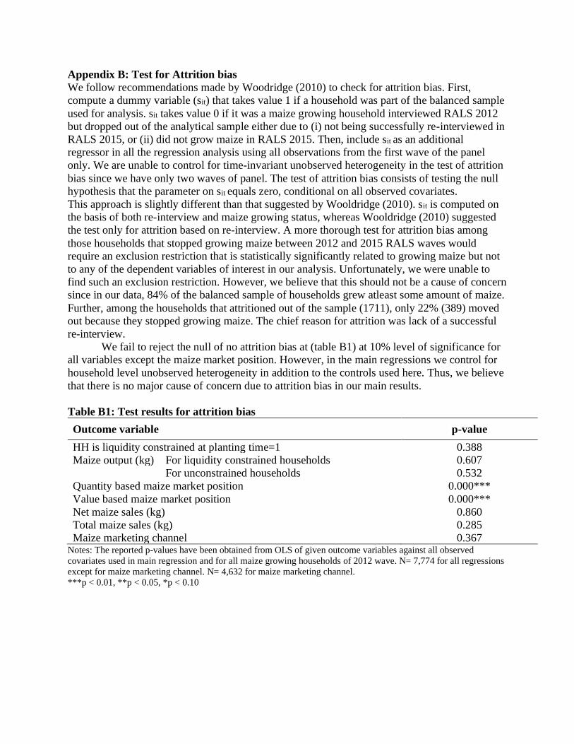
Appendix B: Test for Attrition bias

We follow recommendations made by Woodridge (2010) to check for attrition bias. First,

compute a dummy variable (sit) that takes value 1 if a household was part of the balanced sample

used for analysis. sit takes value 0 if it was a maize growing household interviewed RALS 2012

but dropped out of the analytical sample either due to (i) not being successfully re-interviewed in

RALS 2015, or (ii) did not grow maize in RALS 2015. Then, include sit as an additional

regressor in all the regression analysis using all observations from the first wave of the panel

only. We are unable to control for time-invariant unobserved heterogeneity in the test of attrition

bias since we have only two waves of panel. The test of attrition bias consists of testing the null

hypothesis that the parameter on sit equals zero, conditional on all observed covariates.

This approach is slightly different than that suggested by Wooldridge (2010). sit is computed on

the basis of both re-interview and maize growing status, whereas Wooldridge (2010) suggested

the test only for attrition based on re-interview. A more thorough test for attrition bias among

those households that stopped growing maize between 2012 and 2015 RALS waves would

require an exclusion restriction that is statistically significantly related to growing maize but not

to any of the dependent variables of interest in our analysis. Unfortunately, we were unable to

find such an exclusion restriction. However, we believe that this should not be a cause of concern

since in our data, 84% of the balanced sample of households grew atleast some amount of maize.

Further, among the households that attritioned out of the sample (1711), only 22% (389) moved

out because they stopped growing maize. The chief reason for attrition was lack of a successful

re-interview.

We fail to reject the null of no attrition bias at (table B1) at 10% level of significance for

all variables except the maize market position. However, in the main regressions we control for

household level unobserved heterogeneity in addition to the controls used here. Thus, we believe

that there is no major cause of concern due to attrition bias in our main results.

Table B1: Test results for attrition bias

Outcome variable p-value

HH is liquidity constrained at planting time=1 0.388

Maize output (kg) For liquidity constrained households 0.607

For unconstrained households 0.532

Quantity based maize market position 0.000***

Value based maize market position 0.000***

Net maize sales (kg) 0.860

Total maize sales (kg) 0.285

Maize marketing channel 0.367 Notes: The reported p-values have been obtained from OLS of given outcome variables against all observed

covariates used in main regression and for all maize growing households of 2012 wave. N= 7,774 for all regressions

except for maize marketing channel. N= 4,632 for maize marketing channel.

***p < 0.01, **p < 0.05, *p < 0.10

Appendix C: Computation of expected and realized farmgate FRA and market price of

maize

We refrain from using household level prices in the analysis for the following reasons:

1) Prices in the RALS are only collected for households that sell maize (which comprise of 42%

of the sample), thus generating concerns about incidental truncation if we use these prices.

2) One of our main outcome variables (maize market position) has been computed using

household level prices. Using the same prices as an explanatory variable would lead to

simultaneous bias.

The following constructs of price are used instead:

1) Realized farmgate market price of maize:

We have access to monthly district level retail maize prices for Zambia. These prices were

observed in the nearest district administrative town. We use these prices as estimates of the

maize purchase price offered by private traders to smallholder farmers within a given village.

Prices observed in the month of August of the relevant marketing period are used for the main

analysis because that is when most maize sales have been observed in Zambia across different

years and provinces. Alternatively, average of prices covering different months were also used to

conduct sensitivity analysis (Section 6.4 in main text).

A major limitation with using district-level mean maize price data is that it does not account for

the cost of transporting maize from the village to the town. Thus it does not represent farmgate

prices which are more representative of the prices actually faced by the household. Fortunately,

for farmers whose largest maize sale was made somewhere away from their homestead, RALS

records their transport costs (per kilogram per kilometer) to that point of sale. Additionally,

RALS also records an approximate measure of the cost of transporting maize to the nearest FRA

depot for all households irrespective of whether or not they sell any maize to FRA.

Using this information, we are able to construct a piecewise transport cost of maize for each

cluster in each year. It is expected (and observed in the data) that the cost of transport per unit

per kilometer falls as the distance of sale increases. This is expected because: i) The most

expensive part of transport is that to the nearest feeder road; ii) subsequently, transport on a

feeder road is more expensive than transport on a tarmac road; and iii) there may be fixed costs

of transporting maize, such as a fixed payment made in contracting the transport to a middleman.

This fixed cost then translates into lower per kilometer costs when the distance travelled is

larger. We thus compute a piecewise maize transport cost per kilogram per kilometer for the

categories of 0-5 km, 5-10 km, and more than 10 km. We follow Mason et al. (2015) for

choosing these categories. These categories are reasonable because: (i) most households have

feeder roads within a distance of 0-5 km, (ii) the district town is often located 10 km or further

away from households; and (iii) the categories allowed enough observations in each category to

be able to compute villages level medians. The rule of thumb used while computing the median

was that there are at least five observations per cluster to obtain a median. When this was not

possible, we used the district or the provincial median, whichever permitted at least five

observations. The piecewise cost was used to compute estimated costs of transport (per

kilogram) from the homestead to the nearest district town. We then compute the farmgate market

price of maize by subtracting this cost from the district mean retail maize price.

2) Expected farmgate price of maize:

We use a simple naïve expectation of the maize price to construct the expected market price of

maize. For this we use the district mean retail price of the marketing season immediately before

the marketing season of interest to us. Farmgate prices are computed in the same manner as for

marketing period prices, assuming that transport costs do not change significantly between two

consequent marketing seasons.

3) Expected and realized farmgate FRA price:

The FRA prices are pan-territorial and announced by the government around June-July of every

marketing year. To approximate the expected FRA prices, we simply use FRA’s publicly

announced pan territorial price as of the marketing season prior to the marketing season of

interest to us (in other words the FRA price as of the planting time). The FRA price as of

marketing season was the price announced at the time the smallholders actually sold maize.

In practice, the farmgate prices received by the farmer will be heterogenous given differences in

transport costs from each household. RALS records the cost of transport to the nearest FRA

depot for both the planting and marketing periods. Thus, we are able to obtain good estimates of

the farmgate FRA prices during both the planting and marketing periods.

All prices are adjusted by the consumer price index with a base of 2017.

Table D1. Summary statistics for explanatory and dependent variables used in the analysis

(by RALS wave)

2012 2015

Mean SD Mean SD

Panel A: Explanatory variables

Expected farmgate FRA price (ZMW/kg, 2017=100) 2.21 0.11 1.79 0.10

Expected farmgate market maize price (ZMW/kg,

2017=100) 1.26 0.35 1.60 0.48

Farmgate FRA maize price (ZMW/kg, 2017=100) 2.04 0.07 1.88 0.07

Farmgate maize price (ZMW/kg, 2017=100) 1.41 0.58 1.71 0.41

Commercial basal fertilizer price

(district median, ZMW/kg, 2017=100) 6.13 1.16 5.66 0.71

Wage to weed 0.25 ha (district median, ZMW, 2017=100) 99.7 40.2 92.7 37.5

Maize seed price (district median, ZMW/kg, 2017=100) 9.24 6.11 10.42 5.09

Age of the HH head (years) 46.4 14.6 49.1 14.5

Education of household head (years) 6.15 3.66 6.06 3.67

Male-headed household=1 0.82 0.38 0.80 0.40

Full-time adult equivalents 5.01 2.26 5.19 2.28

Landholding size (ha) 3.15 3.21 3.29 3.40

Tropical livestock units 2.83 8.10 2.80 7.66

Number of plows 0.42 0.86 0.50 0.94

Number of harrows 0.07 0.29 0.08 0.31

Number of ox-carts 0.15 0.40 0.18 0.43

Distance to unpaved road (cluster median, km) 0.94 2.95 1.01 2.40

Distance to paved road (cluster median, km) 28.3 35.0 24.9 30.5

Distance to agricultural market (cluster median, km) 23.4 24.6 23.1 23.8

Number of maize traders visiting village between May-

October 3.71 3.14 3.58 2.59

HH owned a radio at the beginning of marketing period 0.66 0.47 0.64 0.48

HH owned a cellphone at the beginning of marketing

period 0.58 0.49 0.65 0.48

HH owned a bicycle at the beginning of marketing period 0.70 0.46 0.70 0.46

HH experienced moisture shock in current growing

season(t)=1 0.18 0.38 0.48 0.50

Growing season rainfall (mm) 788.4 81.5 833.9 74.9

HH has experienced long term moisture shock (16-yr

MA)=1 0.57 0.49 0.41 0.49

Long run mean growing season rainfall (mm) (16-yr MA) 797.1 63.7 806.9 68.0

HH experienced moisture shock in last growing season (t-

1) (Instrument)=1 1.00 0.05 0.42 0.49

Panel B: Selected dependent variables

Quantity of maize produced by HH (kg) 3777 6667 3835 6710

Quantity of inorganic fertilizer used on maize crop by HH

(kg/ha) 192 214 217 185

HH used improved maize seed =1 0.62 0.49 0.69 0.46

Net maize sales made by the HH (kg) 2282 5793 2390 6229

Number of observations 6063 6063

Notes: HH=household; MA=moving average; ZMW=Zambian Kwacha

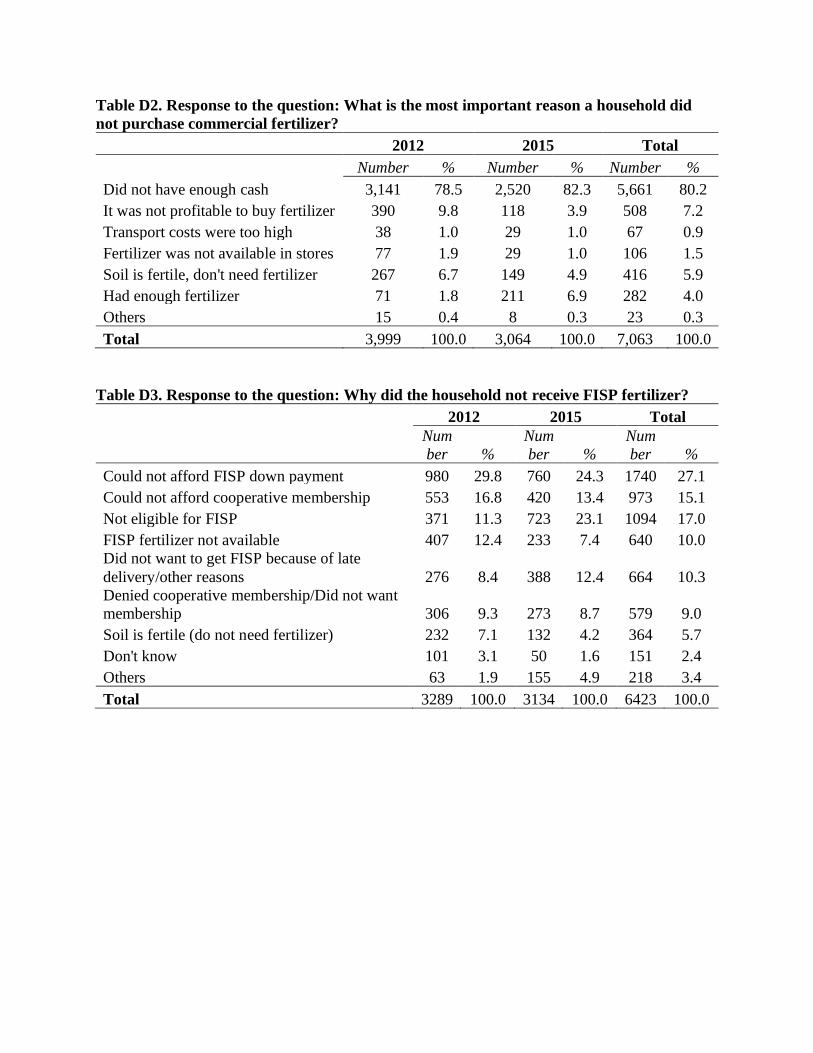
Table D2. Response to the question: What is the most important reason a household did

not purchase commercial fertilizer?

2012 2015 Total

Number % Number % Number %

Did not have enough cash 3,141 78.5 2,520 82.3 5,661 80.2

It was not profitable to buy fertilizer 390 9.8 118 3.9 508 7.2

Transport costs were too high 38 1.0 29 1.0 67 0.9

Fertilizer was not available in stores 77 1.9 29 1.0 106 1.5

Soil is fertile, don't need fertilizer 267 6.7 149 4.9 416 5.9

Had enough fertilizer 71 1.8 211 6.9 282 4.0

Others 15 0.4 8 0.3 23 0.3

Total 3,999 100.0 3,064 100.0 7,063 100.0

Table D3. Response to the question: Why did the household not receive FISP fertilizer?

2012 2015 Total

Num

ber %

Num

ber %

Num

ber %

Could not afford FISP down payment 980 29.8 760 24.3 1740 27.1

Could not afford cooperative membership 553 16.8 420 13.4 973 15.1

Not eligible for FISP 371 11.3 723 23.1 1094 17.0

FISP fertilizer not available 407 12.4 233 7.4 640 10.0

Did not want to get FISP because of late

delivery/other reasons 276 8.4 388 12.4 664 10.3

Denied cooperative membership/Did not want

membership 306 9.3 273 8.7 579 9.0

Soil is fertile (do not need fertilizer) 232 7.1 132 4.2 364 5.7

Don't know 101 3.1 50 1.6 151 2.4

Others 63 1.9 155 4.9 218 3.4

Total 3289 100.0 3134 100.0 6423 100.0

Table D4. Difference in means of key variable between the LC and UC households (LC-

UC)

Variables Criteria 1 or 2 Criterion 1 Criterion 2

Landholding size (ha) -1.05*** -0.89*** -0.94***

Full-time adult equivalents -0.60*** -0.47*** -0.73***

Tropical livestock units -1.49*** -1.25*** -1.30***

Number of plows -0.24*** -0.20*** -0.19***

Number of harrows -0.07*** -0.06*** -0.05***

Number of ox-carts -0.11*** -0.09*** -0.08***

HH owned a bicycle at the beginning

of the marketing period = 1 -0.19*** -0.17*** -0.19***

HH owned a radio at the beginning of

the marketing period = 1 -0.19*** -0.18*** -0.20***

HH owned a cell phone at the

beginning of the marketing period = 1 -0.24*** -0.21*** -0.26***

HH owned a television at the

beginning of the marketing period = 1 -0.19*** -0.17*** -0.17***

Gross per capita income, ZMW -1,823*** -1,593*** -1,587***

Non-farm income earned during peak

maize marketing season, ZMW# -4,065*** -3,547*** -3,240***

Distance to feeder road (cluster

median, km) -0.06 -0.1 -0.05

Distance to paved road (cluster

median, km) 5.46*** 6.24*** 4.39***

Distance to district town (cluster

median, km) 2.75*** 3.01*** 2.64***

Distance to agricultural market

(cluster median, km) 3.08*** 3.60*** 1.45**

No. of maize traders visiting village

during peak maize marketing season# -0.29*** -0.30*** -0.14*

Quantity of fertilizer applied to maize

field, kg/ha -151*** -137*** -225***

HH used improved maize seed=1 -0.32*** -0.28*** -0.52***

Maize productivity (kg/ha) -783*** -694*** -977***

Amount of maize produced per capita -394*** -344*** -317***

Notes: #Peak maize marketing season runs from May-October. The sample consists of all observations in the

analytical sample (N=12126)

*** p<0.01, ** p<0.05, * p<0.1; HH=household; ZMW=Zambian Kwacha

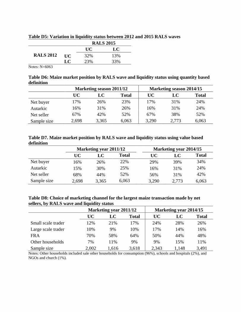
Table D5: Variation in liquidity status between 2012 and 2015 RALS waves

RALS 2015

RALS 2012

UC LC

UC 32% 13%

LC 23% 33% Notes: N=6063

Table D6: Maize market position by RALS wave and liquidity status using quantity based

definition

Marketing season 2011/12 Marketing season 2014/15

UC LC Total UC LC Total

Net buyer 17% 26% 23% 17% 31% 24%

Autarkic 16% 31% 26% 16% 31% 24%

Net seller 67% 42% 52% 67% 38% 52%

Sample size 2,698 3,365 6,063 3,290 2,773 6,063

Table D7. Maize market position by RALS wave and liquidity status using value based

definition Marketing year 2011/12 Marketing year 2014/15

UC LC Total UC LC Total

Net buyer 16% 26% 22% 29% 39% 34%

Autarkic 15% 30% 25% 16% 31% 24%

Net seller 68% 44% 52% 56% 31% 42%

Sample size 2,698 3,365 6,063 3,290 2,773 6,063

Table D8: Choice of marketing channel for the largest maize transaction made by net

sellers, by RALS wave and liquidity status

Marketing year 2011/12 Marketing year 2014/15

UC LC Total UC LC Total

Small scale trader 12% 21% 17% 24% 28% 26%

Large scale trader 10% 9% 10% 17% 14% 16%

FRA 70% 58% 64% 50% 44% 48%

Other households 7% 11% 9% 9% 15% 11%

Sample size 2,002 1,616 3,618 2,343 1,148 3,491 Notes: Other households included sale other households for consumption (96%), schools and hospitals (2%), and

NGOs and church (1%).

Table D9: Descriptive statistics for maize net sellers by maize marketing channel, 2011/12

maize marketing year

% of

net-

sellers

that

sold to

channel

% sold

at

farmgate

Distance covered by

those who travelled

(km)

Farmgate price

(ZMW/kg, 2017=100)

Min Median Max Min Median Max

Small scale trader 17 74 .5 7 202 0.58 1.45 11.5

Large scale trader 10 33 .1 10 420 0.58 1.45 11.7

FRA 64 9 .1 5 180 1.49 2.06 2.38

Other households 9 87 0.5 5.5 130 0.64 1.47 4.16

Sample size 3,618 3,618 2,654 3,618

Notes: Farmgate price is the price received by the household at the point of sale and adjusted for the cost incurred in

transporting the maize from the homestead to the point of sale. It has been computed using prices and costs reported

by the household.

Table D10: Descriptive statistics for maize net sellers by maize marketing channel, 2014/15

maize marketing year

% of

net-

sellers

that

sold to

channel

% sold

at

farmgate

Distance covered by

those who travelled

(km)

Farmgate price

(ZMW/kg, 2017=100)

Min Median Max Min Median Max

Small scale trader 26 66 .15 8 237 0.06 1.40 4.46

Large scale trader 16 30 .1 20 570 0.56 1.40 4.89

FRA 48 11 .15 5 200 0.54 1.74 3.80

Other households 11 85 1 3 60 0.69 1.51 10.7

Sample size 3,618 3,618 2,654 3,618

Notes: Farmgate price is the price received by the household at the point of sale and adjusted for the cost incurred in transporting the maize from the homestead to the point of sale. It has been computed using prices and costs reported

by the household.

Figure D1. Trends in FRA maize purchase, smallholder maize sales, and FRA purchase as

% of smallholder sales, 2007/08 to 2017/18 marketing years Source: Mason and Myers (2013) and Fung et al. (2020), compiled data obtained from the FRA, Crop Forecast

Surveys, Post-Harvest Surveys, and Supplemental Surveys for relevant years.

Note: Estimates of smallholder maize sales were not available for 2016/17.

52%

14%

32%

83%

123%

73%

35%

61%

45%

26%

0

500

1000

1500

2000

2500

2007/08 2008/09 2009/10 2010/11 2011/12 2012/13 2013/14 2014/15 2015/16 2016/17 2017/18

Per

cen

t (%

)

'000

MT

of

mai

ze

FRA maize purchases ('000 MT) Smallholder maize sales ('000 MT)

FRA purchases as % of smallholder sales

Figure D2: Percent of largest maize transactions, by month and marketing channel Source: Author’s calculations from RALS 2012 and 2015 survey data.

Note: 2012/12 maize marketing channel in Panel A and 2014/15 maize marketing channel in Panel B

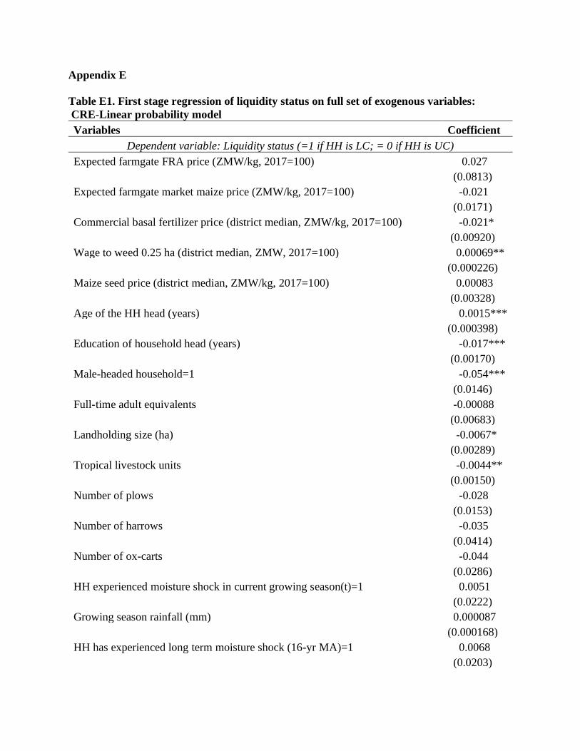
Appendix E

Table E1. First stage regression of liquidity status on full set of exogenous variables:

CRE-Linear probability model

Variables Coefficient

Dependent variable: Liquidity status (=1 if HH is LC; = 0 if HH is UC)

Expected farmgate FRA price (ZMW/kg, 2017=100) 0.027

(0.0813)

Expected farmgate market maize price (ZMW/kg, 2017=100) -0.021

(0.0171)

Commercial basal fertilizer price (district median, ZMW/kg, 2017=100) -0.021*

(0.00920)

Wage to weed 0.25 ha (district median, ZMW, 2017=100) 0.00069**

(0.000226)

Maize seed price (district median, ZMW/kg, 2017=100) 0.00083

(0.00328)

Age of the HH head (years) 0.0015***

(0.000398)

Education of household head (years) -0.017***

(0.00170)

Male-headed household=1 -0.054***

(0.0146)

Full-time adult equivalents -0.00088

(0.00683)

Landholding size (ha) -0.0067*

(0.00289)

Tropical livestock units -0.0044**

(0.00150)

Number of plows -0.028

(0.0153)

Number of harrows -0.035

(0.0414)

Number of ox-carts -0.044

(0.0286)

HH experienced moisture shock in current growing season(t)=1 0.0051

(0.0222)

Growing season rainfall (mm) 0.000087

(0.000168)

HH has experienced long term moisture shock (16-yr MA)=1 0.0068

(0.0203)

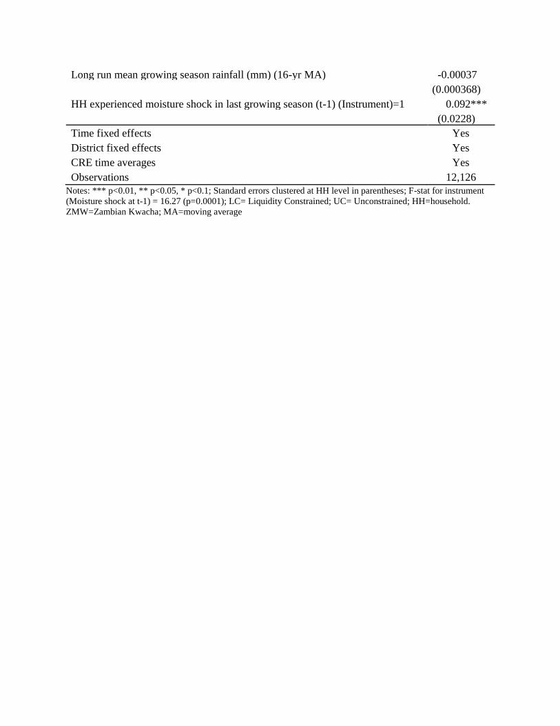
Long run mean growing season rainfall (mm) (16-yr MA) -0.00037

(0.000368)

HH experienced moisture shock in last growing season (t-1) (Instrument)=1 0.092***

(0.0228)

Time fixed effects Yes

District fixed effects Yes

CRE time averages Yes

Observations 12,126

Notes: *** p<0.01, ** p<0.05, * p<0.1; Standard errors clustered at HH level in parentheses; F-stat for instrument

(Moisture shock at t-1) = 16.27 (p=0.0001); LC= Liquidity Constrained; UC= Unconstrained; HH=household.

ZMW=Zambian Kwacha; MA=moving average

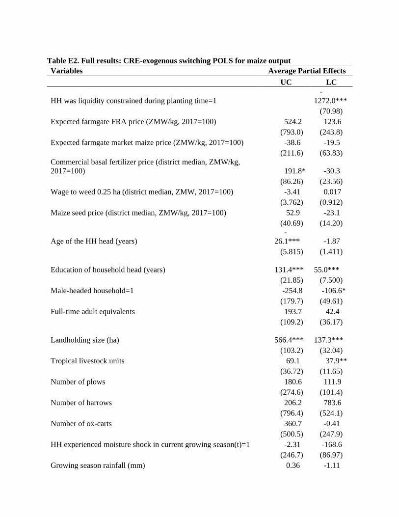
Table E2. Full results: CRE-exogenous switching POLS for maize output

Variables Average Partial Effects

UC LC

HH was liquidity constrained during planting time=1

-

1272.0***

(70.98)

Expected farmgate FRA price (ZMW/kg, 2017=100) 524.2 123.6

(793.0) (243.8)

Expected farmgate market maize price (ZMW/kg, 2017=100) -38.6 -19.5

(211.6) (63.83)

Commercial basal fertilizer price (district median, ZMW/kg,

2017=100) 191.8* -30.3

(86.26) (23.56)

Wage to weed 0.25 ha (district median, ZMW, 2017=100) -3.41 0.017

(3.762) (0.912)

Maize seed price (district median, ZMW/kg, 2017=100) 52.9 -23.1

(40.69) (14.20)

Age of the HH head (years)

-

26.1*** -1.87

(5.815) (1.411)

Education of household head (years)

131.4***

55.0***

(21.85) (7.500)

Male-headed household=1 -254.8 -106.6*

(179.7) (49.61)

Full-time adult equivalents 193.7 42.4

(109.2) (36.17)

Landholding size (ha)

566.4***

137.3***

(103.2) (32.04)

Tropical livestock units 69.1 37.9**

(36.72) (11.65)

Number of plows 180.6 111.9

(274.6) (101.4)

Number of harrows 206.2 783.6

(796.4) (524.1)

Number of ox-carts 360.7 -0.41

(500.5) (247.9)

HH experienced moisture shock in current growing season(t)=1 -2.31 -168.6

(246.7) (86.97)

Growing season rainfall (mm) 0.36 -1.11

(1.751) (0.641)

HH has experienced long term moisture shock (16-yr MA)=1 192.9 -84.4

(281.4) (87.65)

Long run mean growing season rainfall (mm) (16-yr MA) 6.36 2.23

(6.512) (1.242)

Time fixed effects Yes

District fixed effects Yes

CRE time averages Yes

Observations 12,126 Notes: *** p<0.01, ** p<0.05, * p<0.1; Standard errors clustered at HH level in parentheses

LC= Liquidity Constrained; UC= Unconstrained; HH=household. ZMW=Zambian Kwacha; MA=moving average

Table E3. Full results: CRE-endogenous switching POLS for maize output

Variables Average Partial Effects

UC LC

HH was liquidity constrained during planting time=1 -1389.8

(1508.1)

Residuals from first stage regression -27.6 313.1

(2593.1) (732.5)

Expected farmgate FRA price (ZMW/kg, 2017=100) 523.5 131.4

(794.0) (243.6)

Expected farmgate market maize price (ZMW/kg, 2017=100) -37.8 -27.6

(219.4) (67.62)

Commercial basal fertilizer price (district median, ZMW/kg,

2017=100) 192.5 -37.3

(106.2) (30.02)

Wage to weed 0.25 ha (district median, ZMW, 2017=100) -3.43 0.26

(4.351) (1.129)

Maize seed price (district median, ZMW/kg, 2017=100) 52.8 -22.9

(41.23) (14.22)

Age of the HH head (years) -26.1*** -1.41

(6.494) (1.686)

Education of household head (years) 131.8** 49.7***

(47.64) (14.64)

Male-headed household=1 -253.3 -122.8

(244.1) (64.66)

Full-time adult equivalents 193.7 42.5

(109.1) (36.15)

Landholding size (ha) 566.6*** 135.1***

(102.1) (31.84)

Tropical livestock units 69.2 36.7**

(37.72) (11.98)

Number of plows 181.4 102.8

(282.5) (100.4)

Number of harrows 207.2 770.3

(804.5) (524.4)

Number of ox-carts 361.9 -13.5

(523.1) (253.7)

HH experienced moisture shock in current growing season(t)=1 -1.82 -175.0*

(249.5) (85.42)

Growing season rainfall (mm) 0.36 -1.07

(1.845) (0.654)

HH has experienced long term moisture shock (16-yr MA)=1 192.8 -81.0

(281.3) (88.51)

Long run mean growing season rainfall (mm) (16-yr MA) 6.36 2.27

(6.513) (1.248)

Time fixed effects Yes

District fixed effects Yes

CRE time averages Yes

Observations 12,126 Notes: *** p<0.01, ** p<0.05, * p<0.1; Standard errors clustered at HH level in parentheses

LC= Liquidity Constrained; UC= Unconstrained; HH=household. ZMW=Zambian Kwacha; MA=moving average;

FRA=Food Reserve Agency

Table E4. Difference in APEs of key variables on maize output between LC and UC

households, based on CRE-Exogeneous switching POLS

Variables Difference in APE (LC-UC)

Full-time adult equivalents -151.3

(116.4)

Landholding size (ha) -429.1***

(115.3)

Tropical livestock units -31.2

(38.60) Notes: *** p<0.01, ** p<0.05, * p<0.1; Standard errors clustered at HH level in parentheses

LC= Liquidity Constrained; UC= Unconstrained; APE=Average Partial Effects

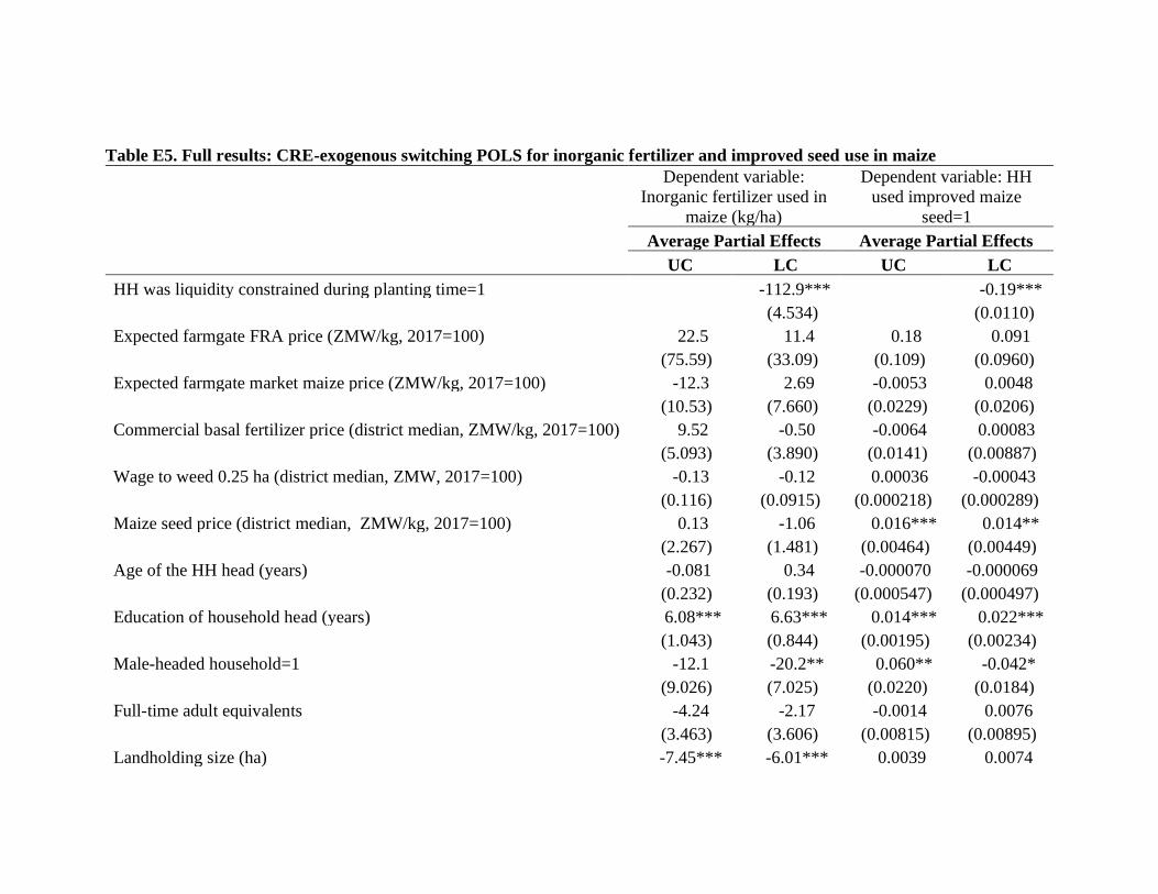
Table E5. Full results: CRE-exogenous switching POLS for inorganic fertilizer and improved seed use in maize

Dependent variable:

Inorganic fertilizer used in

maize (kg/ha)

Dependent variable: HH

used improved maize

seed=1

Average Partial Effects Average Partial Effects

UC LC UC LC

HH was liquidity constrained during planting time=1 -112.9*** -0.19***

(4.534) (0.0110)

Expected farmgate FRA price (ZMW/kg, 2017=100) 22.5 11.4 0.18 0.091

(75.59) (33.09) (0.109) (0.0960)

Expected farmgate market maize price (ZMW/kg, 2017=100) -12.3 2.69 -0.0053 0.0048

(10.53) (7.660) (0.0229) (0.0206)

Commercial basal fertilizer price (district median, ZMW/kg, 2017=100) 9.52 -0.50 -0.0064 0.00083

(5.093) (3.890) (0.0141) (0.00887)

Wage to weed 0.25 ha (district median, ZMW, 2017=100) -0.13 -0.12 0.00036 -0.00043

(0.116) (0.0915) (0.000218) (0.000289)

Maize seed price (district median, ZMW/kg, 2017=100) 0.13 -1.06 0.016*** 0.014**

(2.267) (1.481) (0.00464) (0.00449)

Age of the HH head (years) -0.081 0.34 -0.000070 -0.000069

(0.232) (0.193) (0.000547) (0.000497)

Education of household head (years) 6.08*** 6.63*** 0.014*** 0.022***

(1.043) (0.844) (0.00195) (0.00234)

Male-headed household=1 -12.1 -20.2** 0.060** -0.042*

(9.026) (7.025) (0.0220) (0.0184)

Full-time adult equivalents -4.24 -2.17 -0.0014 0.0076

(3.463) (3.606) (0.00815) (0.00895)

Landholding size (ha) -7.45*** -6.01*** 0.0039 0.0074

(1.424) (1.813) (0.00281) (0.00412)

Tropical livestock units 0.33 -0.13 0.0018 0.0047

(0.796) (0.866) (0.00117) (0.00455)

Number of plows 9.38 11.9 0.021 -0.015

(6.140) (8.384) (0.0139) (0.0266)

Number of harrows 21.7 -7.62 -0.026 -0.037

(20.86) (24.99) (0.0293) (0.0805)

Number of ox-carts -10.6 -6.02 0.021 0.089

(11.94) (14.24) (0.0296) (0.0489)

HH experienced moisture shock in current growing season(t)=1 -19.0 3.89 -0.040 0.033

(11.07) (9.955) (0.0278) (0.0288)

Growing season rainfall (mm) -0.10 0.16 0.000065 0.00057**

(0.0997) (0.0913) (0.000198) (0.000214)

HH has experienced long term moisture shock (16-yr MA)=1 3.37 -8.88 0.087*** -0.037

(8.906) (8.930) (0.0233) (0.0260)

Long run mean growing season rainfall (mm) (16-yr MA) 0.043 0.42* 0.00064 0.00095*

(0.205) (0.194) (0.000502) (0.000464)

Time fixed effects Yes

District fixed effects Yes

CRE time averages Yes

Observations 12,126 Notes: *** p<0.01, ** p<0.05, * p<0.1; Standard errors clustered at HH level in parentheses

LC= Liquidity Constrained; UC= Unconstrained; HH=household. ZMW=Zambian Kwacha; MA=moving average; FRA=Food Reserve Agency

Table E6. Full results: CRE-ordered Probit for quantity-based definition of maize market position

Variables Average Partial Effects

Net-buyer Autarkic Net-seller

Quantity of maize produced, kg -0.00012*** -0.000020*** 0.00014***

(0.0000157) (0.00000147) (0.0000161)

Farmgate maize price (ZMW/kg, 2017=100) -0.0021 -0.00036 0.0025

(0.0116) (0.00195) (0.0135)

Farmgate FRA maize price (ZMW/kg, 2017=100) -0.061 -0.010 0.071

(0.106) (0.0180) (0.124)

Age of the HH head (years) 0.00021 0.000035 -0.00024

(0.000229) (0.0000385) (0.000267)

Education of household head (years) 0.0017 0.00029 -0.0020

(0.00114) (0.000189) (0.00133)

Full-time adult equivalents 0.021* 0.0038* -0.025*

(0.00881) (0.00180) (0.0106)

Male-headed household=1 0.013** 0.0021** -0.015**

(0.00460) (0.000826) (0.00538)

Distance to unpaved road (cluster median, km) # 0.0014 0.00024 -0.0017

(0.00154) (0.000263) (0.00180)

Distance to paved road (cluster median, km) # -0.00030 -0.000051 0.00035

(0.000269) (0.0000467) (0.000315)

Distance to agricultural market (cluster median, km) # 0.00021 0.000035 -0.00024

(0.000338) (0.0000567) (0.000395)

Number of maize traders visiting village between May-October # -0.0018 -0.00030 0.0021

(0.00207) (0.000351) (0.00242)

HH owned a radio at the beginning of marketing period=1 -0.0073 -0.0012 0.0085

(0.0120) (0.00205) (0.0141)

HH owned a cellphone at the beginning of marketing period=1 0.0065 0.0011 -0.0076

(0.0134) (0.00221) (0.0156)

HH owned a bicycle at the beginning of marketing period=1 0.0066 0.0011 -0.0077

(0.0131) (0.00222) (0.0153)

Time fixed effects Yes

District fixed effects Yes

CRE time averages Yes

Observations 12126 Notes: *** p<0.01, ** p<0.05, * p<0.1; Standard errors clustered at HH level in parentheses. HH=household. ZMW=Zambian Kwacha; FRA=Food Reserve

Agency. #The cluster level medians were used for these variables even if they were collected at the household level in order to remove outliers. Cluster here

refers to the standard enumeration area consisting of approximately 20 villages.

Table E7. Full results: CRE-ordered Probit for value-based definition of maize market position

Variables Average partial effects

Net-buyer Autarkic Net-seller

Quantity of maize produced, kg -0.000080*** -0.0000084*** 0.000088***

(0.00000797) (0.000000886) (0.00000839)

Farmgate maize price (ZMW/kg, 2017=100) -0.024 -0.0025 0.027

(0.0136) (0.00145) (0.0150)

Farmgate FRA maize price (ZMW/kg, 2017=100) -0.040 -0.0042 0.044

(0.127) (0.0134) (0.141)

Age of the HH head (years) -0.00045 -0.000047 0.00050

(0.000257) (0.0000271) (0.000284)

Education of household head (years) 0.0024 0.00025 -0.0026

(0.00126) (0.000133) (0.00139)

Full-time adult equivalents 0.018 0.0020 -0.020

(0.0103) (0.00130) (0.0115)

Male-headed household=1 0.012* 0.0013* -0.013*

(0.00559) (0.000596) (0.00617)

Distance to unpaved road (cluster median, km) # 0.00048 0.000051 -0.00053

(0.00188) (0.000198) (0.00208)

Distance to paved road (cluster median, km) # -0.00042 -0.000044 0.00046

(0.000353) (0.0000374) (0.000390)

Distance to agricultural market (cluster median, km) # 0.00012 0.000013 -0.00014

(0.000388) (0.0000409) (0.000429)

Number of maize traders visiting village between May-October # -0.0069** -0.00073** 0.0076**

(0.00249) (0.000267) (0.00275)

HH owned a radio at the beginning of marketing period=1 -0.014 -0.0015 0.016

(0.0138) (0.00143) (0.0153)

HH owned a cellphone at the beginning of marketing period=1 -0.0015 -0.00016 0.0017

(0.0154) (0.00162) (0.0170)

HH owned a bicycle at the beginning of marketing period=1 -0.013 -0.0013 0.014

(0.0151) (0.00153) (0.0166)

Time fixed effects Yes

District fixed effects Yes

CRE time averages Yes

Observations 12126 Notes: *** p<0.01, ** p<0.05, * p<0.1; Standard errors clustered at HH level in parentheses. #The cluster level medians were used for these variables even if they

were collected at the household level in order to remove outliers. Cluster here refers to the standard enumeration area consisting of approximately 20 villages.

HH=household. ZMW=Zambian Kwacha; FRA=Food Reserve Agency

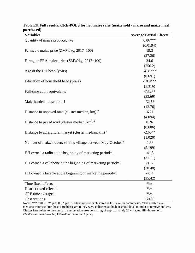
Table E8. Full results: CRE-POLS for net maize sales (maize sold - maize and maize meal

purchased)

Variables Average Partial Effects

Quantity of maize produced, kg 0.86***

(0.0194)

Farmgate maize price (ZMW/kg, 2017=100) 19.3

(27.26)

Farmgate FRA maize price (ZMW/kg, 2017=100) 34.6

(256.2)

Age of the HH head (years) -4.31***

(0.691)

Education of household head (years) -10.9***

(3.316)

Full-time adult equivalents -73.2**

(23.69)

Male-headed household=1 -32.5*

(13.76)

Distance to unpaved road (cluster median, km) # -6.21

(4.094)

Distance to paved road (cluster median, km) # 0.26

(0.686)

Distance to agricultural market (cluster median, km) # -2.63**

(1.020)

Number of maize traders visiting village between May-October # -1.33

(5.199)

HH owned a radio at the beginning of marketing period=1 -41.8

(31.11)

HH owned a cellphone at the beginning of marketing period=1 -9.17

(30.48)

HH owned a bicycle at the beginning of marketing period=1 -41.4

(35.42)

Time fixed effects Yes

District fixed effects Yes

CRE time averages Yes

Observations 12126 Notes: *** p<0.01, ** p<0.05, * p<0.1; Standard errors clustered at HH level in parentheses. #The cluster level

medians were used for these variables even if they were collected at the household level in order to remove outliers.

Cluster here refers to the standard enumeration area consisting of approximately 20 villages. HH=household.

ZMW=Zambian Kwacha; FRA=Food Reserve Agency

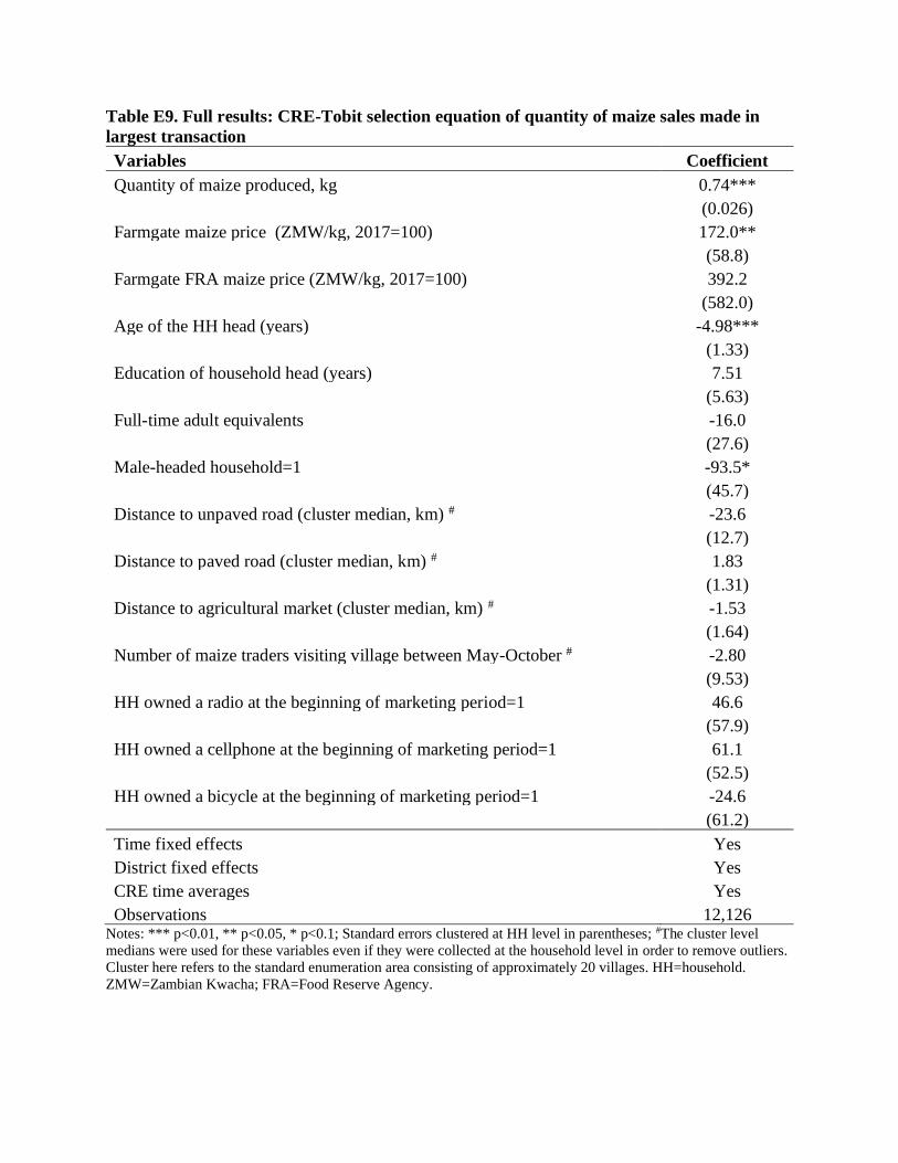
Table E9. Full results: CRE-Tobit selection equation of quantity of maize sales made in

largest transaction

Variables Coefficient

Quantity of maize produced, kg 0.74***

(0.026)

Farmgate maize price (ZMW/kg, 2017=100) 172.0**

(58.8)

Farmgate FRA maize price (ZMW/kg, 2017=100) 392.2

(582.0)

Age of the HH head (years) -4.98***

(1.33)

Education of household head (years) 7.51

(5.63)

Full-time adult equivalents -16.0

(27.6)

Male-headed household=1 -93.5*

(45.7)

Distance to unpaved road (cluster median, km) # -23.6

(12.7)

Distance to paved road (cluster median, km) # 1.83

(1.31)

Distance to agricultural market (cluster median, km) # -1.53

(1.64)

Number of maize traders visiting village between May-October # -2.80

(9.53)

HH owned a radio at the beginning of marketing period=1 46.6

(57.9)

HH owned a cellphone at the beginning of marketing period=1 61.1

(52.5)

HH owned a bicycle at the beginning of marketing period=1 -24.6

(61.2)

Time fixed effects Yes

District fixed effects Yes

CRE time averages Yes

Observations 12,126 Notes: *** p<0.01, ** p<0.05, * p<0.1; Standard errors clustered at HH level in parentheses; #The cluster level

medians were used for these variables even if they were collected at the household level in order to remove outliers.

Cluster here refers to the standard enumeration area consisting of approximately 20 villages. HH=household.

ZMW=Zambian Kwacha; FRA=Food Reserve Agency.

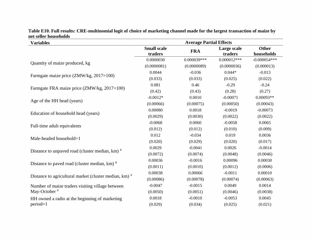
Table E10. Full results: CRE-multinomial logit of choice of marketing channel made for the largest transaction of maize by

net seller households

Variables Average Partial Effects

Small scale

traders FRA

Large scale

traders

Other

households

Quantity of maize produced, kg 0.0000030 0.000039*** 0.000012*** -0.000054***

(0.0000081) (0.0000089) (0.0000036) (0.000013)

Farmgate maize price (ZMW/kg, 2017=100) 0.0044 -0.036 0.044* -0.013

(0.033) (0.033) (0.025) (0.022)

Farmgate FRA maize price (ZMW/kg, 2017=100) 0.081 0.46 -0.29 -0.24

(0.42) (0.43) (0.28) (0.27)

Age of the HH head (years) -0.0012* 0.0010 -0.00071 0.00093**

(0.00066) (0.00075) (0.00050) (0.00043)

Education of household head (years) 0.00080 0.0018 -0.0019 -0.00073

(0.0029) (0.0030) (0.0022) (0.0022)

Full-time adult equivalents -0.0068 0.0060 -0.0058 0.0065

(0.012) (0.012) (0.010) (0.009)

Male-headed household=1 0.012 -0.034 0.019 0.0036

(0.020) (0.029) (0.020) (0.017)

Distance to unpaved road (cluster median, km) # 0.0029 -0.0041 0.0026 -0.0014

(0.0072) (0.0074) (0.0048) (0.0046)

Distance to paved road (cluster median, km) # 0.00036 -0.0016 0.00096 0.00030

(0.0011) (0.0010) (0.0012) (0.0006)

Distance to agricultural market (cluster median, km) # 0.00038 0.00066 -0.0011 0.00010

(0.00086) (0.00078) (0.00074) (0.00063)

Number of maize traders visiting village between

May-October #

-0.0047 -0.0015 0.0049 0.0014

(0.0050) (0.0051) (0.0046) (0.0038)

HH owned a radio at the beginning of marketing

period=1

0.0018 -0.0010 -0.0053 0.0045

(0.029) (0.034) (0.025) (0.021)

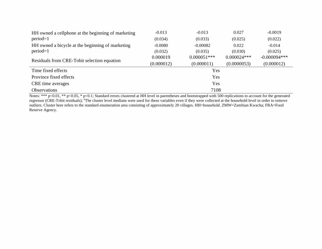
HH owned a cellphone at the beginning of marketing

period=1

-0.013 -0.013 0.027 -0.0019

(0.034) (0.033) (0.025) (0.022)

HH owned a bicycle at the beginning of marketing

period=1

-0.0080 -0.00082 0.022 -0.014

(0.032) (0.035) (0.030) (0.025)

Residuals from CRE-Tobit selection equation 0.000019 0.000051*** 0.000024*** -0.000094***

(0.000012) (0.000011) (0.0000053) (0.000012)

Time fixed effects Yes

Province fixed effects Yes

CRE time averages Yes

Observations 7108 Notes: *** p<0.01, ** p<0.05, * p<0.1; Standard errors clustered at HH level in parentheses and bootstrapped with 500 replications to account for the generated

regressor (CRE-Tobit residuals); #The cluster level medians were used for these variables even if they were collected at the household level in order to remove

outliers. Cluster here refers to the standard enumeration area consisting of approximately 20 villages. HH=household. ZMW=Zambian Kwacha; FRA=Food

Reserve Agency.

Table E11. Full results: CRE-exogenous switching POLS for maize output using alternate

definition of liquidity status

Variables

Average Partial

Effects

UC LC

HH was liquidity constrained during planting time=1

-

1561.5***

(68.91)

Expected farmgate FRA price (ZMW/kg, 2017=100) 391.0 67.4

(408.9) (321.9)

Expected farmgate market maize price (ZMW/kg, 2017=100) 62.2 93.3

(115.9) (70.18)

Commercial basal fertilizer price (district median, ZMW/kg,

2017=100) 36.8 16.5

(36.41) (27.56)

Wage to weed 0.25 ha (district median, ZMW, 2017=100) -3.67 0.088

(2.175) (0.806)

Maize seed price (district median, ZMW/kg, 2017=100) 38.7 -28.3*

(23.86) (12.61)

Age of the HH head (years)

-

16.4*** -1.46

(3.546) (1.290)

Education of household head (years)

108.8*** 14.5*

(14.63) (7.082)

Male-headed household=1

-

385.5*** 53.2

(102.0) (49.79)

Full-time adult equivalents 138.1* 56.9

(66.98) (30.56)

Landholding size (ha)

435.4*** 118.3*

(66.87) (47.61)

Tropical livestock units

68.0** 35.5*

(25.56) (17.42)

Number of plows 314.9 43.4

(185.5) (133.5)

Number of harrows 526.0 4.57

(634.3) (617.9)

Number of ox-carts 463.7 -53.7

(345.3) (340.6)

HH experienced moisture shock in current growing season(t)=1 -111.4 -61.4

(141.9) (89.89)

Growing season rainfall (mm) -1.06 -0.94

(0.920) (0.602)

HH has experienced long term moisture shock (16-yr MA)=1 49.0 9.39

(172.5) (83.34)

Long run mean growing season rainfall (mm) (16-yr MA)

5.70** 2.40*

(1.956) (1.011)

Time fixed effects Yes

District fixed effects Yes

CRE time averages Yes

Observations 12,126 Notes: *** p<0.01, ** p<0.05, * p<0.1; Standard errors clustered at HH level in parentheses

LC= Liquidity Constrained; UC= Unconstrained; HH=household. ZMW=Zambian Kwacha; MA=moving average

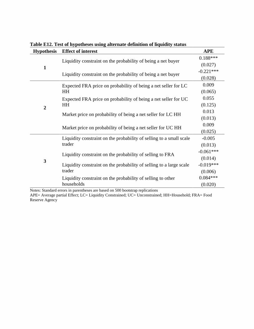
Table E12. Test of hypotheses using alternate definition of liquidity status

Hypothesis Effect of interest APE

1

Liquidity constraint on the probability of being a net buyer 0.188***

(0.027)

Liquidity constraint on the probability of being a net buyer -0.221***

(0.028)

2

Expected FRA price on probability of being a net seller for LC

HH

0.009

(0.065)

Expected FRA price on probability of being a net seller for UC

HH

0.055

(0.125)

Market price on probability of being a net seller for LC HH 0.013

(0.013)

Market price on probability of being a net seller for UC HH 0.009

(0.025)

3

Liquidity constraint on the probability of selling to a small scale

trader

-0.005

(0.013)

Liquidity constraint on the probability of selling to FRA -0.061***

(0.014)

Liquidity constraint on the probability of selling to a large scale

trader

-0.019***

(0.006)

Liquidity constraint on the probability of selling to other

households

0.084***

(0.020) Notes: Standard errors in parentheses are based on 500 bootstrap replications

APE= Average partial Effect; LC= Liquidity Constrained; UC= Unconstrained; HH=Household; FRA= Food

Reserve Agency

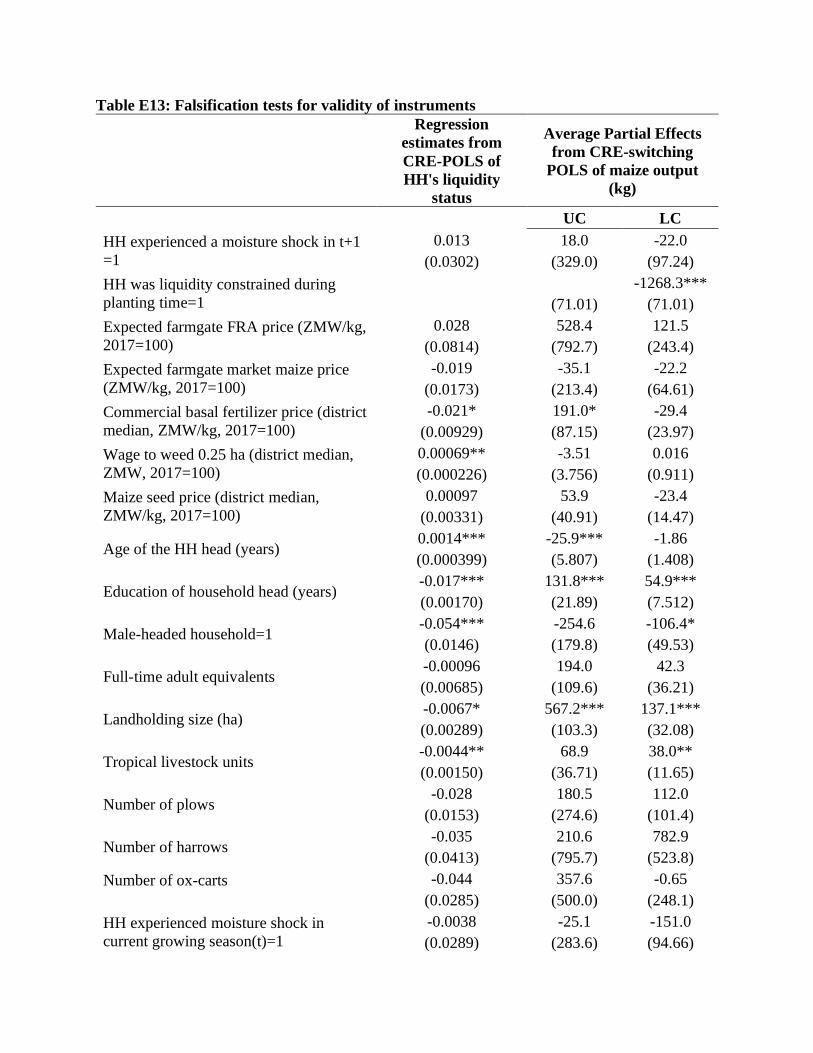
Table E13: Falsification tests for validity of instruments

Regression

estimates from

CRE-POLS of

HH's liquidity

status

Average Partial Effects

from CRE-switching

POLS of maize output

(kg)

UC LC

HH experienced a moisture shock in t+1

=1

0.013 18.0 -22.0

(0.0302) (329.0) (97.24)

HH was liquidity constrained during

planting time=1

-1268.3***

(71.01) (71.01)

Expected farmgate FRA price (ZMW/kg,

2017=100)

0.028 528.4 121.5

(0.0814) (792.7) (243.4)

Expected farmgate market maize price

(ZMW/kg, 2017=100)

-0.019 -35.1 -22.2

(0.0173) (213.4) (64.61)

Commercial basal fertilizer price (district

median, ZMW/kg, 2017=100)

-0.021* 191.0* -29.4

(0.00929) (87.15) (23.97)

Wage to weed 0.25 ha (district median,

ZMW, 2017=100)

0.00069** -3.51 0.016

(0.000226) (3.756) (0.911)

Maize seed price (district median,

ZMW/kg, 2017=100)

0.00097 53.9 -23.4

(0.00331) (40.91) (14.47)

Age of the HH head (years) 0.0014*** -25.9*** -1.86

(0.000399) (5.807) (1.408)

Education of household head (years) -0.017*** 131.8*** 54.9***

(0.00170) (21.89) (7.512)

Male-headed household=1 -0.054*** -254.6 -106.4*

(0.0146) (179.8) (49.53)

Full-time adult equivalents -0.00096 194.0 42.3

(0.00685) (109.6) (36.21)

Landholding size (ha) -0.0067* 567.2*** 137.1***

(0.00289) (103.3) (32.08)

Tropical livestock units -0.0044** 68.9 38.0**

(0.00150) (36.71) (11.65)

Number of plows -0.028 180.5 112.0

(0.0153) (274.6) (101.4)

Number of harrows -0.035 210.6 782.9

(0.0413) (795.7) (523.8)

Number of ox-carts

-0.044 357.6 -0.65

(0.0285) (500.0) (248.1)

HH experienced moisture shock in

current growing season(t)=1

-0.0038 -25.1 -151.0

(0.0289) (283.6) (94.66)

Growing season rainfall (mm) 0.000086 0.31 -1.11

(0.000168) (1.747) (0.649)

HH has experienced long term moisture

shock (16-yr MA)=1

0.0062 192.3 -84.8

(0.0204) (283.1) (88.03)

Long run mean growing season rainfall

(mm) (16-yr MA)

-0.00052 6.81 2.32

(0.000377) (6.555) (1.287)

HH experienced moisture shock in last

growing season (t-1) (Instrument)=1

0.096***

(0.0234)

Time fixed effects Yes Yes

District fixed effects Yes Yes

CRE time averages Yes Yes

Observations 12,126 12,126 Notes: *** p<0.01, ** p<0.05, * p<0.1; Standard errors clustered at HH level in parentheses

LC= Liquidity Constrained; UC= Unconstrained; HH=household. ZMW=Zambian Kwacha; MA=moving average;

FRA=Food Reserve Agency

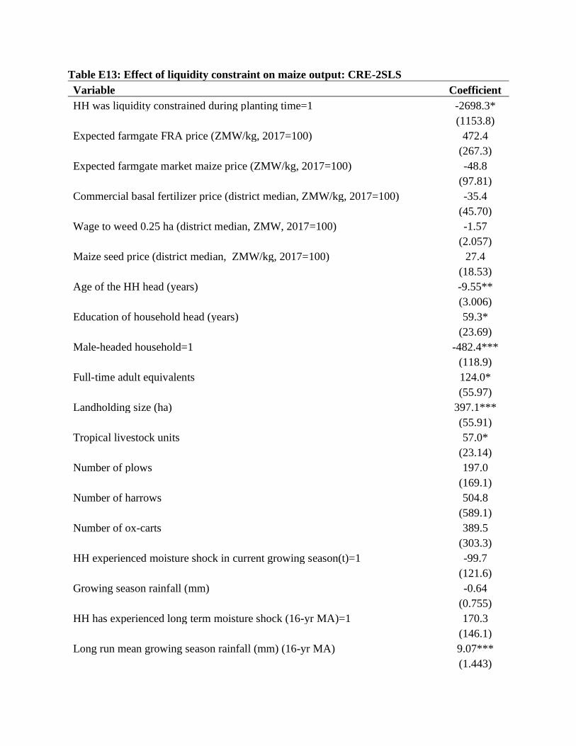
Table E13: Effect of liquidity constraint on maize output: CRE-2SLS

Variable Coefficient

HH was liquidity constrained during planting time=1 -2698.3*

(1153.8)

Expected farmgate FRA price (ZMW/kg, 2017=100) 472.4

(267.3)

Expected farmgate market maize price (ZMW/kg, 2017=100) -48.8

(97.81)

Commercial basal fertilizer price (district median, ZMW/kg, 2017=100) -35.4

(45.70)

Wage to weed 0.25 ha (district median, ZMW, 2017=100) -1.57

(2.057)

Maize seed price (district median, ZMW/kg, 2017=100) 27.4

(18.53)

Age of the HH head (years) -9.55**

(3.006)

Education of household head (years) 59.3*

(23.69)

Male-headed household=1 -482.4***

(118.9)

Full-time adult equivalents 124.0*

(55.97)

Landholding size (ha) 397.1***

(55.91)

Tropical livestock units 57.0*

(23.14)

Number of plows 197.0

(169.1)

Number of harrows 504.8

(589.1)

Number of ox-carts 389.5

(303.3)

HH experienced moisture shock in current growing season(t)=1 -99.7

(121.6)

Growing season rainfall (mm) -0.64

(0.755)

HH has experienced long term moisture shock (16-yr MA)=1 170.3

(146.1)

Long run mean growing season rainfall (mm) (16-yr MA) 9.07***

(1.443)

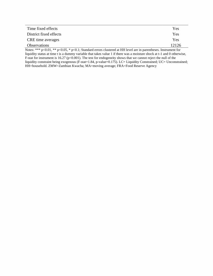
Time fixed effects Yes

District fixed effects Yes

CRE time averages Yes

Observations 12126 Notes: *** p<0.01, ** p<0.05, * p<0.1; Standard errors clustered at HH level are in parentheses. Instrument for

liquidity status at time t is a dummy variable that takes value 1 if there was a moisture shock at t-1 and 0 otherwise,

F-stat for instrument is 16.27 (p<0.001). The test for endogeneity shows that we cannot reject the null of the

liquidity constraint being exogenous (F-stat=1.84, p-value=0.175). LC= Liquidity Constrained; UC= Unconstrained;

HH=household. ZMW=Zambian Kwacha; MA=moving average; FRA=Food Reserve Agency

Table E14: Average partial effects of sensitivity analysis using different measures of prices (CRE-exogenous switching POLS

for maize output)

Model 1 Model 2

UC LC UC LC

HH was liquidity constrained during planting time=1 -1273.0*** -1272.0***

(70.97) (70.97)

Expected farmgate FRA price (ZMW/kg, 2017=100) 525.4 122.3 523.9 119.7

(788.4) (242.9) (789.2) (243.3)

Expected farmgate market maize price (ZMW/kg, 2017=100) -291.1 17.8 -182.0 -6.44

(238.6) (64.48) (235.4) (66.23)

Commercial basal fertilizer price (district median, ZMW/kg,

2017=100) 194.1* -30.4 189.3* -30.4

(85.04) (23.51) (85.58) (23.96)

Wage to weed 0.25 ha (district median, ZMW, 2017=100) -4.30 0.016 -3.83 -0.019

(3.869) (0.861) (3.810) (0.868)

Maize seed price (district median, ZMW/kg, 2017=100) 54.2 -23.0 54.5 -22.6

(41.40) (14.52) (41.43) (14.51)

Age of the HH head (years) -26.2*** -1.87 -26.1*** -1.87

(5.820) (1.410) (5.816) (1.410)

Education of household head (years) 131.3*** 55.0*** 131.5*** 55.0***

(21.86) (7.503) (21.85) (7.499)

Male-headed household=1 -252.6 -106.2* -254.6 -106.4*

(179.7) (49.56) (179.6) (49.55)

Full-time adult equivalents 191.5 41.7 192.7 42.1

(109.6) (36.20) (109.5) (36.22)

Landholding size (ha) 566.3*** 137.4*** 566.3*** 137.3***

(103.2) (32.01) (103.3) (32.05)

Tropical livestock units 70.3 38.0** 69.7 37.9**

(36.75) (11.61) (36.75) (11.64)

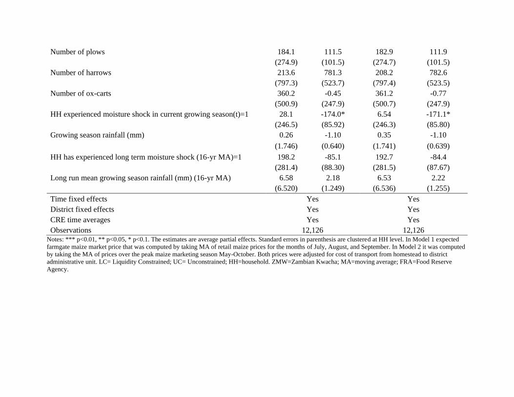
Number of plows 184.1 111.5 182.9 111.9

(274.9) (101.5) (274.7) (101.5)

Number of harrows 213.6 781.3 208.2 782.6

(797.3) (523.7) (797.4) (523.5)

Number of ox-carts 360.2 -0.45 361.2 -0.77

(500.9) (247.9) (500.7) (247.9)

HH experienced moisture shock in current growing season(t)=1 28.1 -174.0* 6.54 -171.1*

(246.5) (85.92) (246.3) (85.80)

Growing season rainfall (mm) 0.26 -1.10 0.35 -1.10

(1.746) (0.640) (1.741) (0.639)

HH has experienced long term moisture shock (16-yr MA)=1 198.2 -85.1 192.7 -84.4

(281.4) (88.30) (281.5) (87.67)

Long run mean growing season rainfall (mm) (16-yr MA) 6.58 2.18 6.53 2.22

(6.520) (1.249) (6.536) (1.255)

Time fixed effects Yes Yes

District fixed effects Yes Yes

CRE time averages Yes Yes

Observations 12,126 12,126

Notes: *** p<0.01, ** p<0.05, * p<0.1. The estimates are average partial effects. Standard errors in parenthesis are clustered at HH level. In Model 1 expected

farmgate maize market price that was computed by taking MA of retail maize prices for the months of July, August, and September. In Model 2 it was computed

by taking the MA of prices over the peak maize marketing season May-October. Both prices were adjusted for cost of transport from homestead to district

administrative unit. LC= Liquidity Constrained; UC= Unconstrained; HH=household. ZMW=Zambian Kwacha; MA=moving average; FRA=Food Reserve

Agency.

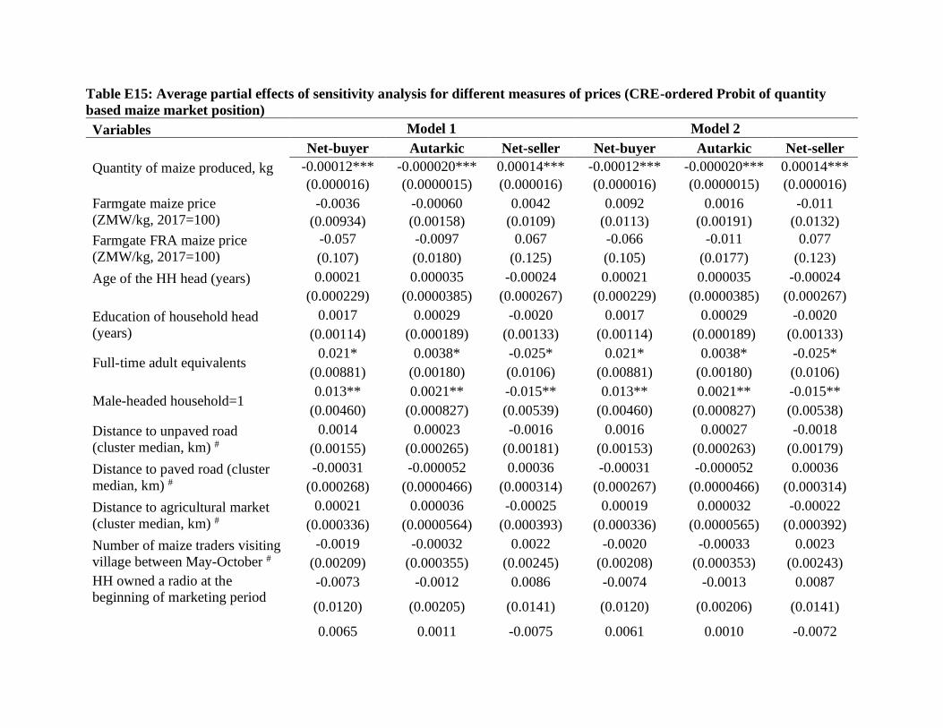
Table E15: Average partial effects of sensitivity analysis for different measures of prices (CRE-ordered Probit of quantity

based maize market position)

Variables Model 1 Model 2

Net-buyer Autarkic Net-seller Net-buyer Autarkic Net-seller

Quantity of maize produced, kg

-0.00012*** -0.000020*** 0.00014*** -0.00012*** -0.000020*** 0.00014***

(0.000016) (0.0000015) (0.000016) (0.000016) (0.0000015) (0.000016)

Farmgate maize price

(ZMW/kg, 2017=100)

-0.0036 -0.00060 0.0042 0.0092 0.0016 -0.011

(0.00934) (0.00158) (0.0109) (0.0113) (0.00191) (0.0132)

Farmgate FRA maize price

(ZMW/kg, 2017=100)

-0.057 -0.0097 0.067 -0.066 -0.011 0.077

(0.107) (0.0180) (0.125) (0.105) (0.0177) (0.123)

Age of the HH head (years)

0.00021 0.000035 -0.00024 0.00021 0.000035 -0.00024

(0.000229) (0.0000385) (0.000267) (0.000229) (0.0000385) (0.000267)

Education of household head

(years)

0.0017 0.00029 -0.0020 0.0017 0.00029 -0.0020

(0.00114) (0.000189) (0.00133) (0.00114) (0.000189) (0.00133)

Full-time adult equivalents 0.021* 0.0038* -0.025* 0.021* 0.0038* -0.025*

(0.00881) (0.00180) (0.0106) (0.00881) (0.00180) (0.0106)

Male-headed household=1 0.013** 0.0021** -0.015** 0.013** 0.0021** -0.015**

(0.00460) (0.000827) (0.00539) (0.00460) (0.000827) (0.00538)

Distance to unpaved road

(cluster median, km) #

0.0014 0.00023 -0.0016 0.0016 0.00027 -0.0018

(0.00155) (0.000265) (0.00181) (0.00153) (0.000263) (0.00179)

Distance to paved road (cluster

median, km) #

-0.00031 -0.000052 0.00036 -0.00031 -0.000052 0.00036

(0.000268) (0.0000466) (0.000314) (0.000267) (0.0000466) (0.000314)

Distance to agricultural market

(cluster median, km) #

0.00021 0.000036 -0.00025 0.00019 0.000032 -0.00022

(0.000336) (0.0000564) (0.000393) (0.000336) (0.0000565) (0.000392)

Number of maize traders visiting

village between May-October #

-0.0019 -0.00032 0.0022 -0.0020 -0.00033 0.0023

(0.00209) (0.000355) (0.00245) (0.00208) (0.000353) (0.00243)

HH owned a radio at the

beginning of marketing period

-0.0073 -0.0012 0.0086 -0.0074 -0.0013 0.0087

(0.0120) (0.00205) (0.0141) (0.0120) (0.00206) (0.0141)

0.0065 0.0011 -0.0075 0.0061 0.0010 -0.0072

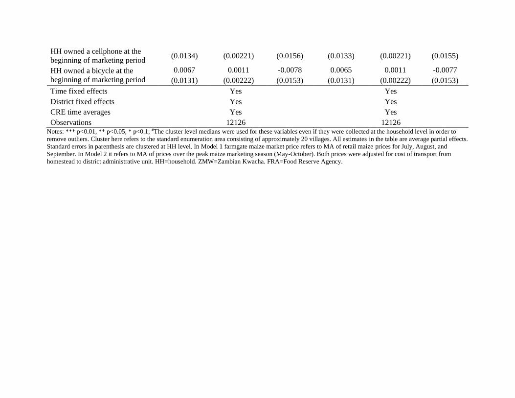
HH owned a cellphone at the

beginning of marketing period (0.0134) (0.00221) (0.0156) (0.0133) (0.00221) (0.0155)

HH owned a bicycle at the

beginning of marketing period

0.0067 0.0011 -0.0078 0.0065 0.0011 -0.0077

(0.0131) (0.00222) (0.0153) (0.0131) (0.00222) (0.0153)

Time fixed effects Yes Yes

District fixed effects Yes Yes

CRE time averages Yes Yes

Observations 12126 12126 Notes: *** p<0.01, ** p<0.05, * p<0.1; #The cluster level medians were used for these variables even if they were collected at the household level in order to

remove outliers. Cluster here refers to the standard enumeration area consisting of approximately 20 villages. All estimates in the table are average partial effects.

Standard errors in parenthesis are clustered at HH level. In Model 1 farmgate maize market price refers to MA of retail maize prices for July, August, and

September. In Model 2 it refers to MA of prices over the peak maize marketing season (May-October). Both prices were adjusted for cost of transport from

homestead to district administrative unit. HH=household. ZMW=Zambian Kwacha. FRA=Food Reserve Agency.