Accepted Manuscript

Smart Data Packet Ad Hoc Routing Protocol

Saman Hameed Amin, H.S. Al-Raweshidy, Rafed Sabbar Abbas

PII: S1389-1286(13)00401-5

DOI: http://dx.doi.org/10.1016/j.bjp.2013.11.015

Reference: COMPNW 5153

To appear in: Computer Networks

Received Date: 7 June 2013

Revised Date: 17 November 2013

Accepted Date: 29 November 2013

Please cite this article as: S.H. Amin, H.S. Al-Raweshidy, R.S. Abbas, Smart Data Packet Ad Hoc Routing Protocol,

Computer Networks (2013), doi: http://dx.doi.org/10.1016/j.bjp.2013.11.015

This is a PDF file of an unedited manuscript that has been accepted for publication. As a service to our customers

we are providing this early version of the manuscript. The manuscript will undergo copyediting, typesetting, and

review of the resulting proof before it is published in its final form. Please note that during the production process

errors may be discovered which could affect the content, and all legal disclaimers that apply to the journal pertain.

Smart Data Packet Ad Hoc Routing Protocol

Saman Hameed Amin1,*, H. S. Al-Raweshidy1, Rafed Sabbar Abbas1

1 Wireless Network and Communications Centre (WNCC),

Electronic & Computer Engineering, School of Engineering and Design, Brunel University, London, UK

Abstract—This paper introduces a smart data packet routing protocol (SMART) based on swarm

technology for mobile ad hoc networks. The main challenge facing a routing protocol is to cope with

the dynamic environment of mobile ad hoc networks. The problem of finding best route between

communication end points in such networks is an NP problem. Swarm algorithm is one of the

methods used solve such a problem. However, copping with the dynamic environment will demand

the use of a lot of training iterations. We present a new infrastructure where data packets are smart

enough to guide themselves through best available route in the network. This approach uses

distributed swarm learning approach which will minimize convergence time by using smart data

packets. This will decrease the number of control packets in the network as well as it provides

continues learning which in turn provides better reaction to changes in the network environment.

The learning information is distributed throughout the nodes of the network. This information can

be used and updated by successive packets in order to maintain and find better routes. This protocol

is a hybrid Ant Colony Optimization (ACO) and River formation dynamics (RFD) swarm algorithms

protocol. ACO is used to set up multi-path routes to destination at the initialization, while RFD

mainly used as a base algorithm for the routing protocol. RFD offers many advantages toward

implementing this approach. The main two reasons of using RFD are the small amount of

information that required to be added to the packets (12 bytes in our approach) and the main idea of

the RFD algorithm which is based on one kind of agent called drop that moves from source to

* Corresponding author. phone +447543386452, e-mail: saman.amin@brunel.ac.uk (Saman Hameed Amin).

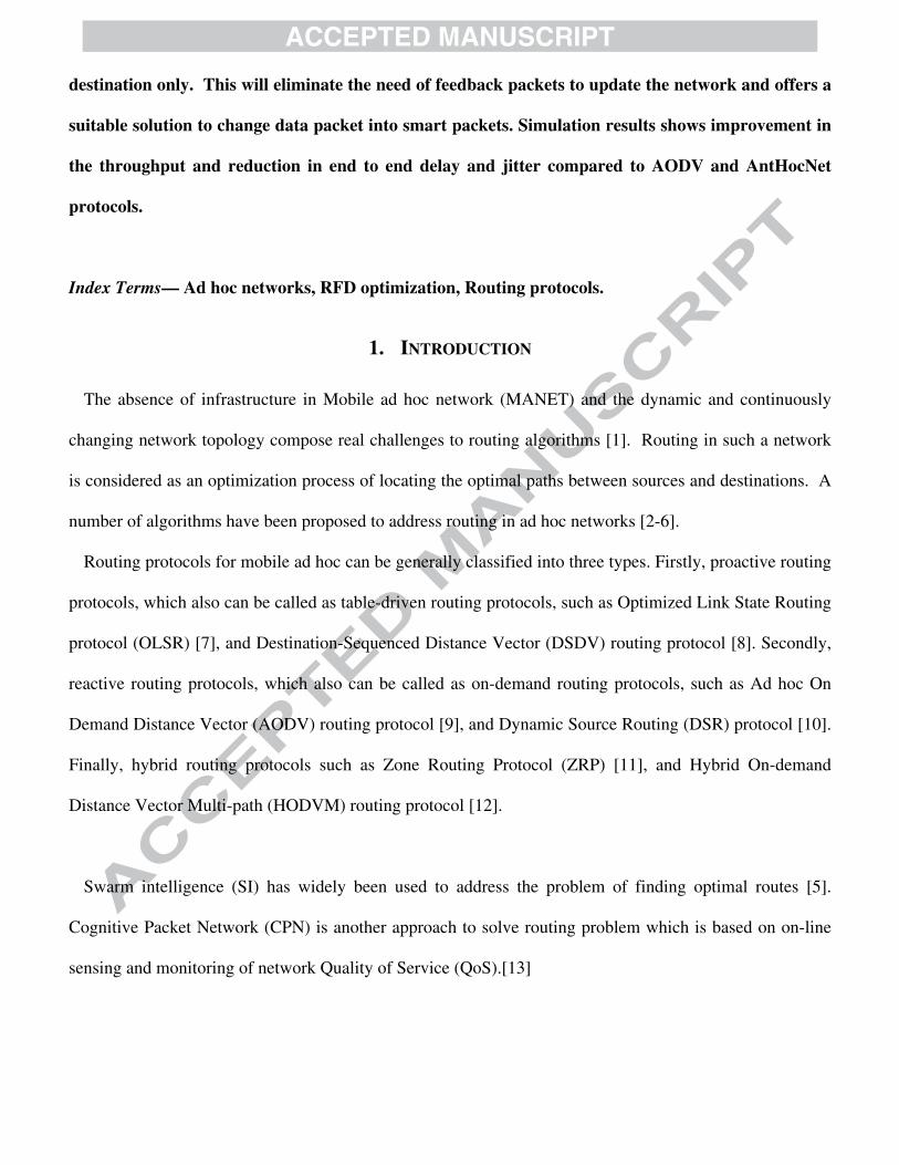
destination only. This will eliminate the need of feedback packets to update the network and offers a

suitable solution to change data packet into smart packets. Simulation results shows improvement in

the throughput and reduction in end to end delay and jitter compared to AODV and AntHocNet

protocols.

Index Terms— Ad hoc networks, RFD optimization, Routing protocols.

1. INTRODUCTION

The absence of infrastructure in Mobile ad hoc network (MANET) and the dynamic and continuously

changing network topology compose real challenges to routing algorithms [1]. Routing in such a network

is considered as an optimization process of locating the optimal paths between sources and destinations. A

number of algorithms have been proposed to address routing in ad hoc networks [2-6].

Routing protocols for mobile ad hoc can be generally classified into three types. Firstly, proactive routing

protocols, which also can be called as table-driven routing protocols, such as Optimized Link State Routing

protocol (OLSR) [7], and Destination-Sequenced Distance Vector (DSDV) routing protocol [8]. Secondly,

reactive routing protocols, which also can be called as on-demand routing protocols, such as Ad hoc On

Demand Distance Vector (AODV) routing protocol [9], and Dynamic Source Routing (DSR) protocol [10].

Finally, hybrid routing protocols such as Zone Routing Protocol (ZRP) [11], and Hybrid On-demand

Distance Vector Multi-path (HODVM) routing protocol [12].

Swarm intelligence (SI) has widely been used to address the problem of finding optimal routes [5].

Cognitive Packet Network (CPN) is another approach to solve routing problem which is based on on-line

sensing and monitoring of network Quality of Service (QoS).[13]

Designing a protocol with two or more QoS constraints is known to be a NP-complete problem [14]. As

problem size increases, the computational complexity of a problem increases, and more time and

computation power are required to solve such a problem. Accordingly, finding shortest path as well as

minimizing delay and avoid congested nodes is an NP-complete problem. Swarm intelligence has been

adapted to solve routing problems due to their efficiency and distributed approach. However, to solve

complex problem using swarm algorithms, the number of iterations required will be proportional to

problem complexity. As the network become more dynamic, the topology will change faster, and more

swarm agents are needed to cope and quickly adapt with this changes in the network. In highly dynamic

environment, more agents are required to detect link qualities in order to find best route. Increasing the rate

of agent, in order to quickly adapt to the changes, will consume more resources. Moreover, each agent will

require a feedback agent to adapt learned parameters which will increase resource consumption.

This paper will propose a smart data packet protocol for mobile ad hoc network using RFD and ACO

algorithms. While the main idea is based on the RFD algorithm, ACO algorithm is used to address the

bottleneck of slow convergence rate of the RFD algorithm in the starting of learning procedure [15]. The

using of ACO algorithm will build a multipath route from source to destination at the beginning of route

setup. We introduce the use of data packet in the learning process of swarm algorithm. Rather than

increasing the number of agents, we use data packets which act like drop agents. We call these packets

“smart data packets” because they behave in smart way by avoiding congested nodes and they incorporate

in the learning process. Moreover, we call them smart to distinguish them from ordinary packets (packets

that are not acting like drops). As these data packet moves in the network, they adapt altitude tables, and

and the network learn about its environment. Using smart data packet will accelerate the sensing and

reaction toward network parameters change.

ACO has been widely used for solving routing problem. In general, in ant based routing protocol, a node

generate forward ant packets to find the destination. Ant packets move around the network in a random

walk to find the destination. This movement is based on some stochastic probability function. When the

destination is found, a backward ant is send from the destination toward the source. As the backward ants

move back to the source, they update the pheromone intensity on the links between the nodes. The path

with higher pheromone intensity will attract more ants and data packets. After a period of time, the optimal

route, depending on the optimization parameters, will be become attractive and will be chosen by the data

packets.

River formation dynamics is a subset of swarm intelligence. It reflects how raindrops on highlands join

together to form rivers [16]. These rivers tend to take shortest path to the sea. Implementing the RFD

algorithm in ad hoc routing protocols provides many advantages. First of all, as there is no backward agent

in the RFD algorithm, it will decrease the total number of control packets in the network. Another

advantage is the simplicity of the algorithm; especially it relates altitudes to nodes rather than links. As

generally the number of nodes is usually less than the number of links in a network. This minimizes the

resource usage. More advantages comes from the fact that the implemented RFD based protocols are using

promiscuous communication mode, so the learning process is not local but all neighbor will be affected by

the learning process. As drops are moving in the network, they update the altitude of the nodes. The drop

carries recent node altitude which will be detected by neighboring nodes. All neighbor nodes will update

the corresponding node altitude in their tables. In other words, one change in a node’s altitude which

announced by one drop packet is corresponding to changes of all links between that node and all its

neighbors. A farther advantage is since RFD uses just drops, which element the need for backward agents

and RFD drops adapts network parameters while they are moving from source(s) to destination(s), this will

offer the opportunity to use data packets and make them act like drops. This allows data packets to guide

themselves and contribute in the learning process. Other protocols usually require backward agents to adapt

routing parameters. With other protocol, assigning a backward agent for each data packet will exhaust the

network. Finally, the amount of control information appended to data packets is small, which make it easy

to integrate the information into the data packets.

This paper is organized as follows. In the next section, related works are given briefly. Section three will

explain the main idea of the RFD algorithm. Section four will explain the proposed protocol. The results

and implementation are given in section five. Finally, a conclusion is given in section six.

2. RELATED WORKS

Routing algorithm is an optimization process that tries to maximize network performance while

minimizing costs. In [9] AODV introduced to solve routing problem. AODV is one of the most popular

classical routing protocols for mobile ad hoc networks. Whenever a node needs to send data to a

destination, and it does not have the valid route to destination, it broadcast a Route Request (RREQ)

message to find the destination. Upon receiving RREQ, Route Replay (RREP) message is send back to the

source. AODV in its original form uses hello message to periodically update its neighbor nodes availability.

Link breakage could be detected if unsuccessful packet transmission occurs or missing hello message. In

case of link failure the node send back a Route Error (RERR) to the source in order to search for new route.

DSR [10] is another type of on demand ad hoc routing protocol which uses dynamic source routing. Unlike

hop to hop routing, source routing protocol adds the complete route path to the packet which gives the

source node complete control on how the packet moves in the network. Ad hoc On demand Multipath

Distance Vector (AOMDV) [17] is a multipath routing protocol which can deal better with mobility than

AODV protocol. AOMDV is an enhancement to AODV where multiple paths are created at route

discovery process. These paths are disjoints and loop free. AOMDV offers better throughput than AODV

regarding and less control packet overhead.

OLSR [7] is a table driven routing protocol. Each node in OLSR uses hello messages to discover its two

hop neighbors using the information carried by hello messages. Each node can select its multipoint re1ay

MPR nodes. MPR nodes are a set of nodes that allow a node to communicate with all its two hop nodes

through these MPR nodes. Each node maintains a table for its neighbors (neighbor table) as well as another

table that contains addresses of it neighbor nodes that have selected it as a MPR (MPR selector table).

Topology control (TC) message are broadcasted periodically and used to build routing tables. DSDV [8] is

another table driven routing protocol where every node keeps a set of distances to every destination

throughout its neighbors. The distance metric can be the number of hops or the end-to-end delay. In order

to keep the distance vector tables up to date, each node periodically broadcasts an update of its shortest

routes to its neighbors.

In [18] the authors analyze the performance of different types of routing protocols used in Wireless

Networked Robotics (WNR). Different scenarios have been proposed to identify the features that affect the

performance of traditional ad hoc routing protocols. The study shows both node capacity and traffic have

the major impact on the performance of routing protocols in WNR. Finally, the study shows that in average

the AODV performance could be considered better than OLSR, DSR, and DSDV.

In [12] HODVM routing protocol for Spatial Wireless Ad Hoc (SWAH) networks is proposed. Spatial

Wireless ad hoc network consists of both mobile and static nodes. Two different protocols have been

adapted to work with backboned network and non-backboned network. Static routing is used for static

nodes, while AODV routing protocol is used for dynamic nodes. Moreover a node behavior distinguishing

algorithm is used to select multiple routes.

Adaptive Neuro-Fuzzy Inference System (ANFIS) has been used by [19] to select a single destination

(server) from a group members belonging to anycast group in mobile ad hoc networks. The protocol uses

three kinds of agents in order to cope with the QoS required. These agents are: static anycast manager

agent, static optimization agent, and mobile anycast route creation agent. Moreover the protocol tries to

select stable routes.

Swarm intelligence is well known optimization algorithm which inspired from the social behavior of

insects and other animals and used to solve optimization problem. Ant Colony Optimization is one of

swarm technology algorithm that has been used to solving routing problems [20]. Ant Based Control

protocol (ABC) [21] is considered the first SI routing protocol for telecommunication networks. ABC

protocol addresses load balance problem using ant agents. The routing protocol is proposed to work on

circuit switched networks. The ants move in one direction from sources to other nodes. As ant moves they

deposit pheromones which will eventually guide data packets. ANTNET [22] is a routing protocol for

packet switch networks. ANTNET uses forward and backward ants based on ACO. ANTNET uses distance

vector for data routing, while it uses source routing for control packets. Thus it will introduce high

overhead especially in large networks. Ant-AODV [23] is a hybrid routing protocol that combines the idea

of AODV and ant-based algorithm. Ant-AODV reduces the end to end delay but it increases the overhead

of route discovery and maintenance. Ant Colony Based Routing protocol (ARA) [24] is using distance

vector routing and supports multipath. It is a reactive routing protocol. The protocol tries to limit the

overhead caused by ants but it losses the proactive feature of ants algorithms. AntHocNet [25] is a

multipath hybrid routing protocol that uses source routing principles combined with ACO. Ants in this

protocol compare both the travel time and hop count with previous visited ants and only broadcast if it is

better. Certain concentrate have been added to decide if ants are going to be broadcasted or unicasted in the

network. AntHocNet protocol features automatic load balancing as backward ants take into account the

delay in each hops. Hello messages have been used to discover neighbor nodes and defuse pheromones.

Link failure is treated using local repair technique. In case of route failure, the node even forward the

packet to next best available neighbor node or it will try to locally repair the route by broadcasting route

repair ant if no more links is available in its route table. On both cases the node informs its neighbor about

link failure. This local repair technique usually will not lead to optimal solution rather than it only finds

another path to the destination.

In [26], Hybrid Routing Algorithm based on ant colony and ZHLS routing protocol for MANET

(HRAZHLS) is proposed. HRAZHLS is based on the Zone based Hierarchical Link State (ZHLS) protocol.

The protocol uses reactive routing outside the zones and used to update its interzone routing table

(InterRT). On the other hand, it uses proactive routing inside the zones to update its intrazone routing table

(IntraRT). Different types of ant are used in the protocol like internal forward ant, external forward ant,

backward ant, notification ant and error ant. Internal forward ants are used to build the proactive tables,

while external forward ants are used to build the reactive routing tables.

BeeAdHoc [27] mimics the beehive in nature. It is relatively a simple algorithm that makes use of a

reactive strategy for agent launching and of source-routing to forward packets. There are two types of bee

agents in the network, short and long distance bee agents. These agents are responsible of exploring the

network and evaluate the quality of their paths in order to update node routing table.

Cognitive Packet Network (CPN) introduced the use of intelligent packets where the capabilities for

routing and control have been moved towards the packets themselves. In CPN, Random Neural Networks

(RNNs) has been used in order to make routing decision. CPN contains three types of packets: Smart

Packets (SPs), Dumb Packets (DPs) and Acknowledgement (ACKs). Packets contain extra fields for

Cognitive Map (CM) and Executable Code. CPN has been used as routing protocol for ad hoc network in

[28, 29].

In [30] the authors present a multiple path approach for CPN in order to perform load balance among all

network nodes. The algorithm carried out in two steps. The first step collect the information about available

multipath in the network then a Hopfield neural network algorithm is used to refine and balance the

distribution of packet around the network.

CPN suffers from high overhead as the amount of control information added to the packet is high. CPN

uses Random Neural Networks (RNN) which adds more computation and resource usage to the network, as

well as vast amount of information (neural networks weights) should be carried by the packets. CPN

protocol infrastructure is completely different from the well-known layered approach of routing

infrastructure. These and other factors led to less interest in CPN.

RFD is a swarm algorithm and has been applied in many combinatorial optimization problems such as

the asymmetric traveling salesman problem [16, 31], Optimal Quality-Investment Tree problem [32],

minimum spanning Tree Problem [33], and others [34-36]. The RFD algorithm mainly uses one kind of

agents which is called drops. Drops moves only from sources to destinations. The RFD algorithm is a

competitor to ACO algorithm and has shown to perform better than ACO in many applications [32, 35].

Our proposed protocol is based on the RFD algorithm. It shares some common feature with the above

presented protocols. It is a hybrid routing protocol. It uses reactive route setup whenever a route is not

available. At the same time it uses hello messages to defuse topology information. Like AntHocNet and

other swarm protocols, SMART protocol uses agents to search for best path. However, SMART protocol

uses data packet to act like drop agents. Unlike other swarm protocols, there is no need for backward

agents. Like CPN, routing decisions are influenced by the information carried by data packets. SMART

protocol distributes the learned information around the network instead of carrying it within the packets.

Only part of the information (altitudes) which reflect the change of network state will be carried by the

packets. Moreover SMART protocol uses distributed learning which is more efficient than local learning

algorithm proposed by CPN.

3. RIVER FORMATION DYNAMICS ALGORITHM

The process of the RFD algorithm starts with initializing the nodes altitude to predetermined positive

value, which reflect flat surface at the beginning. The only exception is the goal point or destination which

will have an altitude value of zero. Destination is considered as sea where the drops should end at. Drops

are generated at the source (sources). At the beginning as all the nodes have same altitude value, the drops

will spread around the flat environment. When some drops find the destination, they fall into it. As they

fall, the nodes altitudes will be eroded. This erosion will create a down slop and throughout many training

cycles the slop will be propagated backward to the source. Drops move according to the following random

probability selection.[16, 33]

(1)

where is the probability of drop k at node i to select node j. Vk is a set of neighbors nodes that can

be visited by the drop from node k. decreasingGradient(i,j) represents the negative gradient between nodes

i and j, which is defined as follows:

(2)

where altitude(x) is the altitude of the node x and distance(i,j) is the length of the edge connecting node i

and node j. At the beginning of the algorithm, all nodes have the same altitude, and the sum of the

decreasing Gradient is also zero. RFD algorithm suggests giving a special treatment to flat gradients,

where the probability that a drop moves through an edge with zero gradient is set to some (non-null) value.

This enables drops to spread around a flat environment, which is mandatory, in particular, at the beginning

of the algorithm.

When a drop moves off a node to lower altitude, the node that the drop moved from will be eroded. The

amount of erosion is proportional to the difference between the altitudes of two nodes.

(3)

Another process which follows the erosion is sediments deposit. There are two type of sediment

depositing, first is the regular periodic addition of sediment to all nodes at constant rate and the second one

is by drops as they move through the network. The amount of sediments that a drop carries throughout its

path from source to that node is accumulative. The amount of sediments that will be deposited at each node

is proportional to the amount that the drop carries.

(4)

Finally, the path from source to destination is analyzed and the stop condition is checked. If the quality is

not good the procedure of drop sending will be repeated until satisfaction quality is reached or when a

maximum number of iteration is reached.

The RFD algorithm shares some aspect with ACO algorithms; the main difference is in the RFD altitude

values are assigned to the nodes themselves while in ACO the pheromone values are assigned to the links

between the nodes. The RFD algorithm could be considered as the gradient version of ACO [15, 35].

However, the RFD algorithm has many advantages over ACO algorithm. The RFD algorithm converges to

better solutions when compared to ACO algorithm [32, 35]. Unlike ACO algorithm, in the RFD algorithm

there is no possibility for local cycles. ACO algorithm suffers from local cycles. In order to prevent local

cycles in ACO, extra techniques are used like buffering visited nodes which has been used in most source

routing ACO based protocols. Source routing protocols suffer from both bandwidth and hop-count

drawback.

The RFD algorithm is more adaptable to changes. Moreover, the RFD algorithm has two different

sedimentation processes. The first is periodical, which is similar to the process of forgetting in ACO. The

second one, which gives advantage to RFD, is the way that RFD tends to cumulate sediment in local

valleys especially if a dead end is reached. In which case the drop stops and drops all of its sediment in that

node causing its altitude to increase which makes it undesirable for other drops to follow. This way of

acting is considered as punishment for bad routes and the probability of other drops to select this

insufficient route will decreases. In spite of all the advantages of the RFD algorithm, it has a main

drawback. The RFD algorithm suffers from slow convergence rate at the beginning of training cycles [15,

33, 34].

To show the slow convergence of the RFD algorithm, a network consisting of a grid of 5 by 10 nodes is

used. Drops are sent from node S (node number 1) to node D as shown in Figure 1. First of all, in order to

test the number of drops needed to create a path, we forced the drops to move along the shortest path in

order to show the delay in path creation. A path is created whenever there is a decreasing slop from the

source to destination. Figure 2 shows the number of drops required to create a path. It shows that at least 8

drops are needed to create a path. This is equal to number of nodes between the source and the destination.

When designing a routing algorithm using the RFD algorithm, special care should be giving to the starting

up mechanism. That is why we have introduced the use of hybrid and RFD and ant protocol in the

beginning of the learning process to overcome this problem.

Figure 3.a shows the effect of variable on the nodes altitude curvature for the shortest path between the

source and the destination. The value of is set to 0.5. It is clear that low value will result in slower

learning at nodes close to the source. Figure 3.b shows the effect of on the curve created by the RFD

algorithm for the same network and same number of drops and we set to 0.5. We can see that the curve

become concave for low values and as the value of increases it converted to convex curve.

A surface that is almost flat near the source increases the probability of drops to move in direction

opposite to the direction of the destination. Moreover, when the surface near the destination becomes

flatter, it gives the opportunity to many nodes to deliver the drop to the destination.

Figure 1. Network topology

Figure 2. Effect of number of drops on nodes altitude

Figure 3. Effect of and on the curvature of altitude surface.

4. SMART DATA PACKET AD HOC ROUTING PROTOCOL

The proposed protocol is a hybrid routing protocol. Hello message has been used to discover neighbor

nodes as well as to defuse information around the network. At the same time, when a node requires a

connection to any other node, it starts a reactive route procedure through broadcasting ant-drop messages

around the network. Smart data protocol is implemented in network layer and uses promiscuous

1 2 3 4 5 6 7 8 9 100

0.1

0.2

0.3

0.4

0.5

0.6

0.7

0.8

0.9

Node number

Alti

tude

=0.5

=0.1

=0.7

Number of drops

Node number

Alti

tude

(a) (b) Node number

Alti

tude

=0 1

=0 5

=0 7

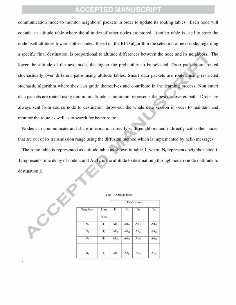
communication mode to monitor neighbors’ packets in order to update its routing tables. Each node will

contain an altitude table where the altitudes of other nodes are stored. Another table is used to store the

node itself altitudes towards other nodes. Based on the RFD algorithm the selection of next node, regarding

a specific final destination, is proportional to altitude differences between the node and its neighbors. The

lower the altitude of the next node, the higher the probability to be selected. Drop packets are routed

stochastically over different paths using altitude tables. Smart data packets are routed using restricted

stochastic algorithm where they can guide themselves and contribute in the learning process. Non smart

data packets are routed using minimum altitude as minimum represents the best discovered path. Drops are

always sent from source node to destination throw-out the whale data session in order to maintain and

monitor the route as well as to search for better route.

Nodes can communicate and share information directly with neighbors and indirectly with other nodes

that are out of its transmission range using the diffusion method which is implemented by hello messages.

The route table is represented as altitude table as shown in table 1 ,where Ni represents neighbor node i.

Ti represents time delay of node i. and ALTij is the altitude to destination j through node i (node i altitude to

destination j)

Table 1: Altitude table

Destinations

Neighbors Time

delay

D1 D2 D3 Dk

N1 T1 Alt11 Alt12 Alt13 Alt1k

N2 T2 Alt21 Alt22 Alt23 Alt2k

N3 T3 Alt31 Alt32 Alt33 Alt3k

Nj Tj Altj1 Altj2 Altj3 Altjk

.

Table 2: My_altitudes table

destination My altitude

D1 Alt1

D2 Alt2

Dk-1 Altk-1

Dk Altk

Another important table is my_altitudes table shown in table 2. This table contains the node itself

altitudes to other destinations.

4.1 Route setup Route discovery starts by checking altitude table for the destination. If the source node has no

information about the route to the destination, it starts broadcasting ant-drop messages. When an

intermediate node receives the ant-drop, it will either unicast or broadcast it. If the intermediate node does

not has a route to the destination it will broadcast it, otherwise it will unicast it. In unicast mode, instead of

using links’ pheromone intensities to route packets, nodes’ altitudes are used to select next node. The

probability selecting of next node is based on equation 1. The decreasing gradient is calculated according to

the following

(5)

where T(k) is the average time that node k needs to send a packet (well be explained in the next

subsection), altituded(j) is altitude of the node j toward destination d.

Due to broadcasting, the number of ant-drops will increased and will build a multipath from the source to

the destination. Ant-drop packet contains a field called travel time. When a node selects the next node it

adds the corresponding next node expected time delay from it altitude table to this field. This accumulated

value will reflect the expected time to travel from the source node to that node. If a node receives another

copy of the same ant-drop packet, having the same sequence number, it will forward it only if the number

of hops or the expected travel time is less than the previous forwarded ant-drop packet. This selective

approach will reduce the overall number of ant-drops in the network which decrease the overhead by

removing unpromising ant-drop packets from the network. Another condition on forwarding a duplicate

copy of the same ant-drop messages is when the first hop that taken by ant-drop is different from the

previous ones. This will allow us to build sufficiently multiple disjoint paths which will add more

protection against link failure [25, 37].

When an ant-drop reaches the destination, it will be converted to a backward ant-drop. This backward

ant-drop moves backward from destination to source depending on the recorded route in the ant-drop

received. This backward ant-drop message will update the altitudes table (my_altitudes) which reflects

nodes altitude to that destination. Intermediate node will calculate updating factor as following

(6)

where is the total accumulated route time by backward ant-drop while traveling back from

destination to node j. thop is a parameter used to represent time required to send a packet in unloaded

condition which is set to 3 ms [25]. hj is number of hops from destination to node j.

The proposed protocol is mainly based on the RFD algorithm, so the idea of ant colony optimization is

adapted to modify altitudes (nodes altitudes) rather than links weights (pheromones intensity). The

backward ant-drop will adopt altitude as following

(7)

where altituded(j) is altitude of the node j (receiver node) toward destination node d. v is the adaptation

factor. Choosing small values for v will lead to rapid change of altitudes and forget its learning information

while larger values lead to more smother changes. Value of 0.9 is chosen.

Each node saves a copy of its altitude before changing and updating by equation 7. Each time a copy of

backward ant-drop passes through a node, equation 7 is computed for the original saved value. Only the

best value is conducted.

When the source node receives backward ant-drop packet, it starts sending data packets.

4.2 Smart data packets and drops routing In order to find better paths and maintain the route, drop packets are sent throughout data session. Data

packets are being used to act like drops and called smart packets. As long as data packet travels from source

to destination it is better to use these data packets to reinforce the learning process. This makes data packets

detect congested nodes and update altitudes. Therefor successive data packet will select different route as

the altitudes change. Smart data packets act like drops; they search and react to network condition as well

as they contribute in the learning process of the network. The learning information is stored in the altitude

tables throughout the network. Although drops and smart packets act the same way, smart data packet are

routed in in restricted way. This minimizes the latency as well as decreases the probability of data packet

being sent far away from the destination. At the same time drops will continue discovering other parts of

the network.

The rate of drops is set to one drop per 0.5 second. The drops are propagated according to the gradient

probability function in equations 5 and 1. Using time delay parameter will reduce the probability of

selecting congested nodes. The more congested the node, the more it is not preferred to be selected. The

higher value T(k) is representing higher distance according to the RFD algorithm and the node is not

preferable to be next forwarding node.

Each drop packet contains a field that represents the recent altitude of sender node. Drops change node

altitudes by the process of eroding and adding sediments. The node new altitude to the final destination of

drop is attached to the drop packet. All neighbor nodes will update their tables according to the new altitude

carried by the drop packet. This is acts like a distributed learning procedure where one change affects a

group of nodes. Each node also monitors its sent packets. Unlike ant based algorithms where an ant updates

specific link pheromone intensity that is moving along, one drop alters a node altitude and all neighbors are

updating their tables according to this change.

Figure 4. Time between sending a packet and receiving a copy of it.

When a node starts sending a packet, it computes how much time is needed for the next node to send it

again as shown in Figure 4. The time delay is the amount of time between sending the packet and receiving

a copy when transmitted by next node. Whenever this time is available, upon successful reception of the

transmitted packet using promiscuous mode, the node updates the average time delay value. It keeps

tracking of this by computing the running average of the time needed by its neighbor to forward its packets.

This value is stored in altitude table.

(8)

where Ck(t) is new delay in node k at time t, Tk is time delay for node k. T initially is set to be equal to the

time required by an unloaded node to send a packet. γ is a parameter regulating how quickly the formula

adapts to new information (set to 0.7). Using this type of distance will help in selecting uncongested node.

When a node becomes more congested, its time delay will increase. This makes it undesirable and nodes

will forward packets to other neighbor. This reflects how water drops behave in nature. When a group of

Time Time Time

Sender 1st neighbor node 2nd neighbor node

Sending packet

Sending packet

Received via promiscuous mode

rivers pour in the same valley, and the amount of outgoing water from the valley is less than the amount of

incoming water, a water lake is created. As the water level is increased, the water on some edges will start

to leak out to the other sides of the mountains around the lake. Water drops that fall on places close to these

edges will follow to other sides with the leaking water rather than to the valley.

When drops move in the network they erode the altitudes of the nodes. The amount of erosion is

proportional to altitude difference between sender and receiver nodes. The selected forward node altitude is

taken from the altitude table and used to calculate the gradient. The erosion is calculated using

(9)

(10)

where erosiond(j) is the amount of erosion at the node j toward destination d, altituded(j) is the altitude of

node itself, k is the next selected node. α is a positive constant number between 0 and 1 which reflects

erosion factor (set to 0.7). High value of α will lead higher erosion and missing of optimal solution. While

very low value my lead the algorithm to fall in local minimum. Due to nodes mobility and dynamic

infrastructure of mobile ad hoc network, low values for α are not preferred.

At the same time drops add sediment to node altitude. The amount of sediment is proportional to the

amount of sediment carried by the drop as well as inversely proportional to the altitude difference of the

node and next node altitudes. When the altitude difference is low which represent flat surface, the drop will

deposit more sediment.

(11)

(12)

β and ε are constants controlling the amount of sediments deposit (set to 0.1 and 0.1 respectively). Carried

sediment reflects the path characteristic. Paths with higher slops will result in more carried sediment.

Setting β and ε to high value will lead to quickly depositing sediments. This will lead to a convex

topographical structure where the altitudes around the source are less curvature. While lower values will

lead to concave structure and the flat part will close to the destination. Lower value will make drops search

around the destination for better delivery nodes. Flat surface around the source will increase the probability

of sending data packet to directions opposite to the destination direction, which in turn will move them far

away from the destination.

The sediment carried by the drop to next node is

(13)

Another type of sediment adding occur periodically every fixed amount of time

(14)

where w is a set of all known destinations. θ is the amount of sediment to be add( set to 0.01). θ acts as

forgetting factor. High value will quickly erase learned information, especially for recent learned paths.

Low value is chosen because we don’t want to corrupt recent learned information and there are other

methods that will also help in adapting the information like the punishment procedure if a link broken. The

time period between regular additions is set to 1 second.

To implement smart data protocol, extra fields should be added to data packets in order to act like drops.

It is significant to keep the added information to data packets as small as possible and not to overload the

data with many extra bytes. Drop packet themselves are small in size. Three parameters have been added to

data packet, altitude, carried sediment and the sender address each of them are four bytes in size.

Smart data packets should have the opportunity to discover new routes. This means they should move

like drops. In order to limit them from exploring long paths and keep them close to the best known path,

nodes that have minimum altitude and less congested are having minimum distance and considered as best

shortest path, data packets are routed using greedy and restricted method. Data packets use altitude table

and move according to the following random probability selection function below.

(15)

where is a constant number greater than one, and is set to 4 to achieve the greedy movement. V(j) is set of

neighbor node of node j.

Usually the number of data packets is much higher than drop packets. This high number of data packets

could ruin the learning process especially as these packets are moving in a greedy way. This reflects

flooding in nature. To limit the erosion that is occurring due to this high number of data packet, the

percentage of erosion and sedimentation by data packets is reduced.

4.3 Hello messages and information diffusion

Hello messages are used to propagate information around the network. Essentially, hello message is used

to declare node presence; moreover it is used to carry information about node neighbors. Hello message is

extended to carry K elements from its altitude table (K=10 is used). Using this idea the altitudes of the

nodes will be distributed around the network.

The receiving node will update the altitude toward this node (my_altitudes) and updates its altitude to

those destinations that are carried by the hello messages by a factor proportional to the difference between

node altitude and received altitude.

(16)

helloaltitude d is the altitude of destination d in hello message, μ is the adaptation constant (set to 0.1).

Although distributing information by hello messages help to form paths to destinations but it has some

drawbacks. The reliability of this information is not high. First, this information does not address the

congestion in the nodes. Second, since hello messages are sent every hello interval period this information

may be out of date.

4.4 Link failure

The protocol detects route failure in two ways. The first one is by detecting the missing of hello message

from a neighbor for a time period more than allowed hello loss. Allowed hello loss period is set to be twice

as hello interval which is inherited from AODV protocol. The second way of detecting link failure is

through missing acknowledgment after sending data or drop packet.

If a route failure occurred, the node deactivates the route in route altitude table. Then it updates its

destination attitude table. If the loss of a neighbor affects the table then it will broadcast a notification to its

neighbors.

Whenever the reason of link failure is due to the failed transmission of data packet, than the node will try

to send the packet to the next best neighbor. At the same time if the altitude of this neighbor is higher than

the altitude of the node itself, it will change its altitude to the same amount of the next best neighbor. In a

worse case, if there is no node to deliver the packet to, the node will return the packet to its sender. In this

case the altitude of the node to this destination becomes one. The previous node and all neighbors will

update their tables with the new altitude value of that node and will route further new packets according to

new altitudes. When a node becomes a dead end, there is an opportunity that this node and its neighbors are

constructing a local valley. Local valleys should be filled quickly as they work as attracting zones for

packets which in turn increases the number of lost packets. The above procedure will prevent wasting many

packets on local valleys. Without this procedure, the number of packet required to fill a valley is at least

equal to the number of nodes between the dead end node and a node with valid link to the destination. To

prevent wasting this amount of packets, this procedure will damp it with the same packet that is returned.

At the same time, the packet is not lost and the learning process is going on.

4.5 Smart data packets routing example The section explains how smart data packets are routed in the network. In Figure 5.a, node 1 sends

packets to node 9. The numbers over each node represent nodes altitude toward node 9. Red arrows

represent best route. To explain different approaches of how the routing problem is solved and the

advantages of the proposed protocol, we will assume all protocols start by selecting the route 1-2-4-7-9.

After selecting the route, we assume that node 4 has involved in a communication session with node 10.

Then node 4 moves far from node 2 and the link is broken between them. Node 4 becomes congested and

the route is not available as shown in Figure 5.b.

Starting with AODV protocol, when node 4 becomes congested, AODV has no mechanism to detect

congestion and it waits until route break occurs. After all, a new route set up procedure is required.

If an ACO based protocol like AntHocNet is used; first let us assume that the rate of ant generation is

equal to one ant per second. When route break occur and as AntHocNet is multipath protocol, node 2

forwards the packet to next available node (node 5) and the route become 1-2-5-7-9. Both nodes 5 and 7 are

in the transmission of node 4 and will be affected by it, however the protocol does entirely depends on ant

agents to detect network status. The protocol will wait for at least one second, if not more, until an ant pass

through the route and change the pheromone intensities of the links in that route (by the backward ant).

In the proposed protocol, as node four becomes congested, its distance become higher (equations 5 and

8). The time needed to send the packet from node 2 to node 4 will increase. Node 1 will update the time of

node 2 according to equation 8.

Accordingly, in node 1, the probability of selecting node 2 or 3 changes (probability of selecting node 2

decreased depending on the delay). When the link breaks, node two will forward the data to node 5 at same

time it changes its altitude to be equal to node 5 (0.45). Node 1 will get a copy of the sent packet and

update the altitude of node 2 in its altitude table to 0.45. Now the altitude of node 3 is less than node 2,

therefor node 3 will have higher probability to be selected as next node and the route will change to 1-3-5-

7-9. The data packets behave in smart way as they always try to avoid congested area in the network. An

important point here is all the above occurred during data packets sending. There is no need to wait for one

second like ACO based protocol to send an agent and detect the change in the network parameters. The

altitudes have been changed with data packets. No need for feedback agents. Moreover, the changes not

only affect the node but it will propagate backward and affect previous nodes’ altitudes. It should be noted

that the process here is not only message forwarding, it is a distributed learning and optimization technique

which continuously learn and react according to network status to find best route. Another advantage of

using smart packets is it will minimize convergence time. For example, if the number of ants required in

order to find a solution (best route) was 100 ants, with a rate of one ant per second, this will take 100

second. As for SMART protocol with the same rate of agents (drops) and with data rate of five packets per

second, the time will be shorter. Each second there will be one drop and five smart data packets that act like

drops, which means there will be six drops per second. The convergence time will be about 16.66 second.

Figure 5. An example of smart data packet routing.

(a) (b)

5. IMPLEMENTATION AND SIMULATION RESULTS

The performance of the proposed protocol was evaluated by comparing it with AntHocNet (swarm based

multipath routing protocol) and standard AODV protocols (with local repair) [9]. AODV is chosen because

it is a well-known and almost considered as reference protocol in this research area. AntHocNet protocol

is a swarm based algorithm and is chosen because it outperforms many ant routing protocols in many

aspects [38, 39].

Simulation results are generated using OMNet++ as simulation software. A model for AntHocNet

protocol was implemented based on [25]. As for the AODV protocol, the INETMANET add-on package of

the OMNet++ is used. An important point worth mentioning here is we tried to match the setting of all

protocols as possible. We have set the rate of ant’s generation equal to the rate of drop’s generation. We

equaled the rate of hello messages for all protocol as well. As we used the standard AODV with no

modification as a comparison routing protocol, we kept with its setting and any other setting required for

proposed protocol was inherited form AODV protocol.

5.1 Simulation environments In our experiment, three scenarios have been implemented to test our protocol. Previous studies show that

ad hoc network can produce best performance if the number of neighbors is between six to eight [21].

However, we have chosen node density close to 6.25 in order to have good connectivity. With this node

density, there is a good probability for a node to have multipath to its destination. At the same time, as the

environment become more aggressive, nodes speed increases, the probability of link failure increases,

which provide a good environment to test our protocol.

In the first scenario, 32 nodes have been randomly placed in a 600 *600 m2 environment. Simulation time

was set to 200 seconds. The simulations are repeated for twenty times with different seeds.

The medium access control protocol is the IEEE 802.11 DCF. Packet size is 512 bytes. Five mobile

nodes selected randomly to act as sources and five other nodes acts as receivers. Each node generates a

packet every 0.2 second. As described in [18], with this size of network (medium size) and low data rate,

the probability of route failure increases which offers more aggressive environment to test the protocol. The

network remains silent in the first second. The nodes start sending data at third second and keep sending

until the end of simulation, which gives one second for some hello packet to be generated before starting

data session. Data traffic is generated using constant bit rate (CBR) UDP traffic sources. Two mobility

models are used, random waypoint (RWP) model and Gauss Markov (GM) model [40], to test the

performance of the protocols.

In the second scenario, the number of nodes increased to 64 and to keep node density almost equal to the

first test, the area is increased to 850*850 m2. This scenario is used to test the scalability of the protocol,

keeping the same node density and increasing network size. Simulation time was set to 400 seconds. The

simulations are repeated for twenty times with different seeds. The number of sources is increased to ten

and the number of destination nodes is increased to ten as well. Only random waypoint (RWP) model has

been used.

In order to test the performance of the protocol under different node densities, a third scenario is

introduced. This scenario is similar to the first one, except that we fixed the speed of the nodes to 10 m/s.

The number of nodes varied from 20 up to 100 nodes. Random waypoint (RWP) model is used in this

scenario. Moreover, to analyze the impact of the traffic load on the performance of the protocol, we use

this scenario to test the protocols under different traffic loads. We set the number of nodes to 32, and

increase the load by increasing the number of packets sent per second (packets rate).

Other common parameters for all scenarios are set as following. Each node has a radio propagation range

of 150m and channel capacity of 54 Mb/s. Hello time intervals is set to 0.5 second. Pause time is set

randomly between 0.1 and 1 second.

The following end to end network characteristic has been studied [25, 41].

1-Throughput: is the measure of the total number of successful delivered data bits over simulations time

for a specific node, averaged over the number of source-destination pairs.

2-End to end delay: is the measure of average delay of data packets. This is the time from sending the

packet from the application layer at the source node to the time that the packet arrives to the application

layer at the destination node, averaged over the number of source-destination pairs.

3-Jitter: is the variation of packet delay which is averaged over the number of source-destination pairs,

averaged over the number of source-destination pairs.

4-Routing overhead is the total number of control packets sent divided by the number of data packets

delivered successfully.

5- Number of route requests: is the total number of route request generated by specific node (RREQ in

AODV, forward ant broadcast in AntHocNet, and ant-drop broadcast in SMART), averaged over the

number of source-destination pairs.

6- Average number of buffered packets per node: is the total number of packets that have been buffered

in MAC layer averaged over number of nodes.

5.2 Results Figure 6 and 7 show the throughputs of SMART routing protocol compared with AODV and

AntHocNet protocols under different nodes speed. It is clearly seen that SMART protocol performs better

than both AODV and AntHocNet. Figure 6 shows that a significant increase in throughput can be achieved

by using SMART protocol. For 10 m/s the throughput increased up to 17% over AODV and 13% over

AntHocNet under RWP mobility model. When nodes become more mobile, the altitude table, which

reflects the topology, will need more updates, therefor the throughput decreases. Comparing the results of

the network under RWP mobility with GM mobility, we can see the protocol preforms better under RWP

mobility. There are two main reasons for that. Firstly, in RWP mobility, the nodes tend to move toward the

center of the simulation area and move away from the simulation area boundary. This will leads to

fluctuation in node density and as a result, the path lengths become shorter. The nodes are better distributed

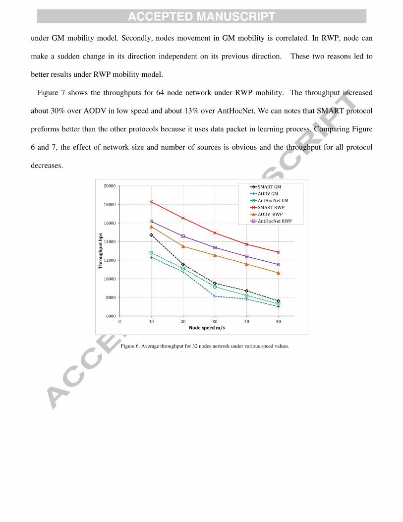
under GM mobility model. Secondly, nodes movement in GM mobility is correlated. In RWP, node can

make a sudden change in its direction independent on its previous direction. These two reasons led to

better results under RWP mobility model.

Figure 7 shows the throughputs for 64 node network under RWP mobility. The throughput increased

about 30% over AODV in low speed and about 13% over AntHocNet. We can notes that SMART protocol

preforms better than the other protocols because it uses data packet in learning process. Comparing Figure

6 and 7, the effect of network size and number of sources is obvious and the throughput for all protocol

decreases.

Figure 6. Average throughput for 32 nodes network under various speed values.

Figure 7. Average throughput for 64 nodes network under various speed values

The end to end delay for the first scenario is shown in Figure 8 and for the second scenario is shown in

Figure 9. Both figures show more than 96% enhancement in end to end delay. SMART data protocol

produces better results than the others. The main factors that contribute in network latency and jitter are

congestion, queuing and route changing. In AODV most of the delay occurs due to route setup and

broadcasting of control packets and route maintenance as well as queuing of data packets. At the same

time, the criteria of selecting next forwarding node and finding the optimal path from source to destination

also contributes in the delay. SMART protocol minimizes the number of broadcasting, and tries to select a

non-congested node. If a node had a route failure, it forwards the packet to other best node. At the same

time when a packet is moving around the network, the process of learning is still carried on and nodes

update their altitude tables continually.

AntHocNet forward data depending only on regular pheromone (there are two type of pheromones tables

in AntHocNet, regular and virtual) which mostly trained by backward ants. This table may not have all

possible paths to destinations as this require huge number of ants and training cycles, so in many situation

route break occurs. The method of packet forwarding and continues real time learning of SMART protocol

leads to better performance. Smart data packets allow the network to learn more rapidly and the packets can

find other routes. Another important factor, if a better route is found, the AntHocNet needs many ants to

enhance the weight of the route to be selected. SMART protocol is based on RFD and adopts faster.

Comparing Figure 8 with Figure 9, the effect of network size and number of sources is obvious. As the

network become larger and number of source nodes increases, the probability of link breakage increases

and the repair time will be longer as well as the network becomes more congested. As the network size

increases, the search space for finding better routes also increases.

Figure 8. Average end to end delay for 32 nodes network under various speed values.

Figure 9. Average end to end delay for 64 nodes network under various speed values.

Figure 10. SMART protocol end to end delay under various speed values.

The end to end delay of the SMART protocol is very low. Figure 10 shows the effect of speed on the end

to end delay for the first and second scenarios. For 32 node network, the average end to end delay under

both RWP and GM mobility is between 0.89 up to 1.3 millisecond and increasing slowly as node speed

increases. The delay is higher in 64 node network and starts from 1.4 millisecond up to 1.8 millisecond.

According to network setting, the time needed Tp to send a packet in our network as we use two way

handshaking (DATA- ACK) could be calculated as below [42-44]

Tp = TDIFS +TSIFS+ TBO + TDATA +TACK (17)

where TDIFS is the Distributed InterFrame Space time ( 34 μs), TSIFS is Short InterFrame Space (SISF)

time (9 μs), TBO is backoff interval time (min 67.5 μs) , TDATA is MAC Protocol Data Unit ( MAC PDU)

plus Physical Layer Convergence Protocol( PLCP ) header plus PLCP preamble (for 512 byte plus extra

fields, it will be 106.6 μs), and TACK is acknowledgement time (24 μs). For 32 node network, in average,

the end to end delay time is more than four successful data transmission time, while it is equal to about

seven successful transmissions in 64 nodes network.

The extra bytes that been added to smart data packet will add about 2 microsecond to the transmission

time of data packet, which is less than 1% of data transmission duration. If a separate control packet has

been used for this information it would introduced a lot of delay to the network. Sending 12 bytes as

separate packet including MAC control overhead will require 161 microsecond. Apart from the total

number of control packet required if a separate control packet is used, the reduction in time is obvious. As

an example of reduction of control packets, the average throughput at 10m/s for 32nodes network is

18281bps, the average delivered packet to each destination is 883. If separate packet used, this would

require extra 883 control packets to be delivered to each destination. In spite the extra time needed to

transmit a smart data packet, its efficiency is cleared from the above.

Figure 11 and 12 show the jitter for the first and second scenarios respectively. Again SMART protocol

overcome both protocols and has less jitter. Variation in network structure due to nodes mobility causes

link breakage. Both AODV and AntHocNet have route recovery mechanism which consists of queuing and

rebroadcasting. SMART protocol is based on instantaneous data packet rerouting to other better route in

case of route failure. As the data packets moves from source to destination, all nodes within the route will

continue their learning process by the data packet. Moreover, all nodes that are neighbors to the route will

also learn as the process of learning in SMART protocol is distributed. An extra point to address here, data

packets are routing themselves through multipath to the destination through nodes around best discovered

path. This will load balance the network, as well as it creates a valley like structure which its lowest end is

at the destination. When a node in-between becomes unreachable, the data packets should easily find

another path to the destination.

Figure 11. Average jitter for 32 nodes network under various speed values.

Figure 12. Average jitter for 64 nodes network under various speed values.

Both AntHocNet and SMART protocols are hybrid routing protocols and they send control messages

throughout the entire data session in order to maintain the route between the source and the destination.

This could produce more overhead in the network and costing the network to use more resources. Figure 13

shows the control packet overhead of the three protocols for both the first and second scenarios under RWP

mobility. SMART protocol generates more control overhead than AODV protocol, however the control

overhead is less than AntHocNet. The absence of backward agent and the use of SMART data packets led

to less control overhead than AntHocNet.

Figure 13. Control packet overhead under various speed values.

The third scenario is used to study the effect of node density on the protocol performance. Figure 14

shows the effect of node density on network throughput. When the number of nodes is less than 40 nodes in

the network, the connectivity of the network is degraded and the throughput decreased. When the number

increases over 60 nodes, the network become more congested and the throughout decreases again. From the

figure it is clear that the proposed protocol overcome both other protocol throughout all number of nodes.

Figure 15 shows the end to end delay for various numbers of nodes. When there are few nodes in the

network, the number of route failure increases. For each route failure, the AODV route recovery requires

more time which causes more delay because of broadcasting. AntHocNet has faster recovery procedure [7],

however it also uses broadcasting algorithm whenever a route break occurs. SMART protocol usually do

not buffer data packet, unless if the destination is unreachable. As the network become denser, the number

of nodes involved in a route may increase in both AODV and AntHocNet. The cost of broadcasting

increases as well as the probability of collision increases. SMART protocol is more efficient in searching

for better routes, and it minimizes the number of broadcasting in the network. It can be seen that the end to

end delay at low node density is high. This occurs because at low node density the probability of the

destination being unreachable is high. The delay occurs usually as a consequence of queuing and

broadcasting. Putting in mind, in our protocol queuing occurs only at the original source when the

destination is unreachable and all the nodes around the original source do not have a route to the

destination. In other words all the nodes around the source have an altitude equal to one. This situation is

rarely occurs unless the source node is isolated alone or with only few nodes. The reason that reduces this

situation is hello message and distributed learning. Whenever a drop is moving through the network it

erodes its path, and node surrounding the path will be also eroded by distributed learning. Hello message is

also eroding the altitudes of neighbor nodes. However, two methods are participating in increasing the

altitudes, the sediment addition, and the punishment process. The ratio of sediments addition is always low.

The punishment in our approach is limited to two nodes to decrease network traffic and prevent the losing

of learned information. Limiting the punishment procedure to two nodes, described in section 4.4, will

require many packets to set the altitude of all the nodes around the source to one. Moreover, as explained in

section 4.3 that hello messages erode altitude of neighbor nodes, if a node with an altitude less than one

broadcasts its hello messages to those neighbor that have been punished, it will result in decreasing their

altitudes. This will also decrease the probability of bringing the altitudes of all nodes around the source to

one. Another factor also contribute in decreasing this probability is when a node joins these group, and it

has an altitude lower than one to the desired destination, it will decrease the altitude of its neighbor in the

group when it send hello messages or when a data activity occur at that node as all the neighbors will listen

to its activity (promiscuous mode updating). Smart data packets as well as drops may be forwarded to that

node. If this node joins another group to the original source group and become a link between them, smart

data packets and drops will try to find a route to destination through this new group, and in case if there is a

valid path to the destination from that node, they will follow that route. Even if the topology of these nodes

and links changed and become expire, these smart packets will adapt and search for a link to the

destination. After all, this is why we can see that the end to end delay in our protocol is always low, as data

packets are always being sent and searching and creating new routes. The probability of queuing as well as

broadcasting is low and data packets may be deleted in case if they reach a dead end or when maximum

number of hops is reached. Throughout all our simulation, we observed that the maximum number of

broadcasting for any source (route set up) in each simulation was always less or equal to three. This

indicates that the probability of queuing is very low. Table 3 shows the average number of route request

generated by source nodes in AODV protocol compared to SMART protocol. AODV has a local route

repair procedure and the average number of route repair at each node in the network is also shown in the

table. The results are for scenario one and for random way point mobility. The effectiveness of the RFD

algorithm can be seen as drops and smart packets are always moving and searching for a route rather than

depending on a recovery mechanism as in AODV or AntHocNet. Whenever a link becomes expire, drops

as well as smart packets will follow to new offered paths to search for destination. Similarly, when a flow

of water drop is closed, water drops will follow new paths until they reach the sea. In their way to the sea,

they will continue their erosion and sedimentation process, i.e. the learning process is never stops.

Figure 14. Network throughput under various numbers of nodes.

Figure 15. Network end to end delay under various numbers of nodes.

Table 3: Average number of route request for the first scenario under RWP mobility Speed (m/s)

10 20 30 40 50 Number of Route discovery for AODV protocol

19.95 26.45 32.24 35.81 39.28

Local route repair for AODV protocol 2.18 2.62 2.48 2.59 2.70 Number of Route discovery for SMART Protocol

1.22 1.24 1.34 1.38 1.46

Number of Route discovery for AntHocNet 12.54 16.38 22.02 26.66 28.56

Figure 16 shows the effect of increasing traffic load on the proposed protocol compared to AODV and

AntHocNet protocols. The number of packet per second varied from 10 packets to 60 packets per second. It

is clear that the throughput of SMART protocol is better than others especially in high traffic load at 60

packets per second. Figure 17 shows the end to end delay under variable packet rate. The negative slope of

the AODV end to end delay at the beginning is due to the rate of encountering route failure for low data

rate is high or the probability of finding difficulties to build valid route to the destination [18].

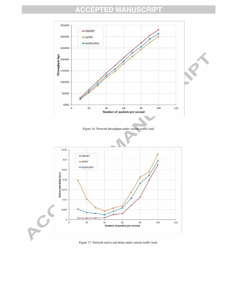
Figure 16. Network throughput under various traffic load.

Figure 17. Network end to end delay under various traffic load..

(a)

(b)

Figure 18. Low packet data rate example

Table 4 shows the average number of packets buffered at MAC layer per second. It is clear that the main

cause of delay at high data rate is because of buffering at MAC layer. The design of MAC protocol and the

detection of link failure at MAC layer caused more packets to be buffered and added delay to the network.

At low data rate, the source of delay is due to network layer protocol. The number of packets buffered at

MAC layer is very low.

Figure 18 shows an example of the reason that at low data rate the delay is high in AODV protocol and

decreasing as the data rate increases until certain data rate. In figure 18a, the ratio of packets that suffering

from delay to overall number of packets passing through a node is ½ (1 packet delayed per 2 packets).

When the data rate increases, as in figure 18b the ratio will decreases and as example become ¼ so the

average delay decreases as data rate increases until certain data rate. It should be noted that when a source

node is dealing with route recovery the new packets will be buffered and network layer until a route will be

found.

Data packets

Time

Time required until link break detection Route recovery

time

Link break

Time

The SMART protocol rarely has route recovery; however the delay of link breakage detection occurs as it

is related to MAC and link layers protocols. The link break detection depends on the retry limit constant set

at MAC layer which define how many time the node will try to send the packet before reporting link

breakage. The delay in AODV will be higher as route recovery based on broadcasting while the SMART

protocol will forward the packet to next available node.

At a certain data rate, the traffic in the network will suffer more delay as network become congested and

the number of packet that are buffered in both network and MAC layer increases resulting in more end to

end delays. As this delay at high data rate is inherited from MAC layer protocol, we preferred to use low

data rate to show the delay caused by network protocol.

Table 4: AVERAGE NUMBER OF BUFFERED PACKETS PER NODE

data rate (p/s)

10

20

30

40

50

60

70

80

90

100

AODV 0.105469 0.196387 0.394531 14.28906 39.97314 246.9009 886.0752 1209.461 1344.716 1791.581

SMART 0.098633 0.188477 0.323242 14.35547 25.60547 170.8007 533.3301 743.4785 1274.656 1622.425

6. CONCLUSIONS

In this paper we have proposed smart data routing protocol for mobile ad hoc networks based on the RFD

algorithm. RFD is a swarm algorithm inspired by the way rain drops make rivers.

The learning in the RFD algorithm is feed forward and eliminates the need for backward packets. This

reduces the number of control packets in the network and offers a good opportunity to change and

implement smart data packets.

Data packet in the proposed protocol could be ordinary or smart packet. The proposed protocol is flexible

and can work on both smart and ordinary data packet. Smart packets carry extra fields in order to contribute

in learning process which as result affects the movement of the packets in the network. These extra fields

are appended to the end of IP packet header, which adds more compatibility and flexibility to the protocol

in order to handle ordinary data packets.

Our results show that smart data protocol performs better than AODV and AntHocNet. In average, the

throughput is increased and both end to end delay and jitter decreased.

REFERENCES

[1] P. Lalbakhsh, B. Zaeri, A. Lalbakhsh and M.N. Fesharaki, '"AntNet with Reward-Penalty Reinforcement Learning," Computational Intelligence, Communication Systems and Networks (CICSyN), 2010 Second International Conference on, 2010, pp. 17-21.

[2] A. Boukerche, B. Turgut, N. Aydin, M.Z. Ahmad, L. Bölöni and D. Turgut, '"Routing protocols in ad hoc networks: A survey," Computer Networks, vol. 55, no. 13, 2011, pp. 3032-3080.

[3] Kwang Mong Sim and Weng Hong Sun, '"Ant colony optimization for routing and load-balancing: survey and new directions," Systems, Man and Cybernetics, Part A: Systems and Humans, IEEE Transactions on, vol. 33, no. 5, 2003, pp. 560-572.

[4] S. Marwaha, J. Indulska and M. Portmann, '"Biologically Inspired Ant-Based Routing in Mobile Ad hoc Networks (MANET): A Survey," Ubiquitous, Autonomic and Trusted Computing, 2009. UIC-ATC '09. Symposia and Workshops on, 2009, pp. 12-15.

[5] G.S. Sharvani, N.K. Cauvery and T.M. Rangaswamy, '"Different Types of Swarm Intelligence Algorithm for Routing," Advances in Recent Technologies in Communication and Computing, 2009. ARTCom '09. International Conference on, 2009, pp. 604-609.

[6] B. Kalaavathi, S. Madhavi, S. Vijayaragavan and K. Duraiswamy, '"Review of ant based routing protocols for MANET," Computing, Communication and Networking, 2008. ICCCn 2008. International Conference on, 2008, pp. 1-9.

[7] P. Jacquet, P. Muhlethaler, T. Clausen, A. Laouiti, A. Qayyum and L. Viennot, '"Optimized link state routing protocol for ad hoc networks," Multi Topic Conference, 2001. IEEE INMIC 2001. Technology for the 21st Century. Proceedings. IEEE International, 2001, pp. 62-68.

[8] C.E. Perkins, P. Bhagwat, C.E. Perkins and P. Bhagwat, '"Highly dynamic Destination-Sequenced Distance-Vector routing (DSDV) for mobile computers;" SIGCOMM Comput.Commun.Rev., vol. 24, no. 4, 1994, pp. 234-244.

[9] C.E. Perkins and E.M. Royer, '"Ad-hoc on-demand distance vector routing," Mobile Computing Systems and Applications, 1999. Proceedings. WMCSA '99. Second IEEE Workshop on, 1999, pp. 90-100.

[10] D.B. Johnson, D.A. Maltz and J. Broch, '"DSR: The Dynamic Source Routing Protocol for Multi-Hop Wireless Ad Hoc Networks," Addison-Wesley, 2001, pp. 139-172.

[11] P. Samar, M.R. Pearlman and Z.J. Haas, '"Independent zone routing: an adaptive hybrid routing framework for ad hoc wireless networks," IEEE/ACM Trans.Netw., vol. 12, no. 4, 2004, pp. 595-608.

[12] L. Guo, L. Zhang, Y. Peng, J. Wu, X. Zhang, W. Hou and J. Zhao, '"Multi-path routing in Spatial Wireless Ad Hoc networks," Computers & Electrical Engineering, vol. 38, no. 3, 2012, pp. 473-491.

[13] E. Gelenbe, Zhiguang Xu and E. Seref, '"Cognitive packet networks," Tools with Artificial Intelligence, 1999. Proceedings. 11th IEEE International Conference on, 1999, pp. 47-54.

[14] Z. Wang and J. Crowcroft, '"Quality-of-service routing for supporting multimedia applications," Selected Areas in Communications, IEEE Journal on, vol. 14, no. 7, 1996, pp. 1228-1234.

[15] P. Rabanal and I. Rodriguez, '"Hybridizing River Formation Dynamics and Ant Colony Optimization,"in Advances in Artificial Life. Darwin Meets von Neumann, vol. 5778. George Kampis, et al. , Springer Berlin Heidelberg, 2011, pp.424-431.

[16] P. Rabanal, I. Rodríguez and F. Rubio, '"Using River Formation Dynamics to Design Heuristic Algorithms," Unconventional Computation Lecture Notes in Computer Science, vol. 4618, 2007, pp. 163-177.

[17] M.K. Marina and S.R. Das, '"On-demand multipath distance vector routing in ad hoc networks," Network Protocols, 2001. Ninth International Conference on, 2001, pp. 14-23.

[18] B. Blanco, F. Liberal and I. Taboada, '"Suitability of ad hoc routing in WNR: Performance evaluation and case studies," Ad Hoc Networks, vol. 11, no. 3, 2013, pp. 1165-1177.

[19] V.R. Budyal and S.S. Manvi, '"ANFIS and agent based bandwidth and delay aware anycast routing in mobile ad hoc networks," Journal of Network and Computer Applications, no. 0.

[20] G. Singh, N. Kumar and A. Kumar Verma, '"Ant colony algorithms in MANETs: A review," Journal of Network and Computer Applications, vol. 35, no. 6, 2012, pp. 1964-1972.

[21] R. Schoonderwoerd, J.L. Bruten, O.E. Holland and L.J.M. Rothkrantz, '"Ant-based load balancing in telecommunications networks," Adapt.Behav., vol. 5, no. 2, 1996, pp. 169-207.

[22] G. Di Caro and M. Dorigo, '"Mobile agents for adaptive routing," System Sciences, 1998., Proceedings of the Thirty-First Hawaii International Conference on, vol. 7, 1998, pp. 74-83.

[23] S. Marwaha, Chen Khong Tham and D. Srinivasan, '"Mobile agents based routing protocol for mobile ad hoc networks," Global Telecommunications Conference, 2002. GLOBECOM '02. IEEE, vol. 1, 2002, pp. 163-167.

[24] M. Gunes, U. Sorges and I. Bouazizi, '"ARA-the ant-colony based routing algorithm for MANETs," Parallel Processing Workshops, 2002. Proceedings. International Conference on, 2002, pp. 79-85.

[25] G.D. Caro, F. Ducatelle and L.M. Gambardella, '"AntHocNet: An adaptive nature-inspired algorithm for routing in mobile ad hoc networks," European Transactions on Telecommunications, vol. 16, SEP 2005, pp. 443-455.

[26] M. Rafsanjani, S. Asadinia and F. Pakzad, '"A Hybrid Routing Algorithm Based on Ant Colony and ZHLS Routing Protocol for MANET,", vol. 120, 2010, pp. 112-122.

[27] H.F. Wedde, M. Farooq, T. Pannenbaecker, B. Vogel, C. Mueller, J. Meth and R. Jeruschkat, '"BeeAdHoc: an energy efficient routing algorithm for mobile ad hoc networks inspired by bee behavior," Proceedings of the 2005 conference on Genetic and evolutionary computation, 2005, pp. 153-160.

[28] E. Gelenbe and R. Lent, '"Power-aware ad hoc cognitive packet networks," Ad Hoc Networks, vol. 2, no. 3, 2004, pp. 205-216.

[29] R. Lent, '"Smart packet-based selection of reliable paths in ad hoc networks," Design of Reliable Communication Networks, 2005. (DRCN 2005). Proceedings.5th International Workshop on, 2005, pp. 5 pp.

[30] L. CHEN, H. JI, Y. LI and X. LI, '"Multi-path routing based on load-balance for cognitive packet networks," The Journal of China Universities of Posts and Telecommunications, vol. 18, no. 5, 2011, pp. 71-75.

[31] Hifza Afaq , Sanjay Saini, '"On the Solutions to the Travelling Salesman Problem usingNature Inspired Computing Techniques," IJCSI International Journal of Computer Science Issues, vol. 8, no. 4, July 2011, pp. 326 -334.

[32] P. Rabanal, I. Rodríguez and F. Rubio, '"Applying RFD to Construct Optimal Quality-Investment Trees," J.UCS Journal of Universal Computer Science, vol. 16, no. 14, May 2010, pp. 1882-1901.

[33] P. Rabanal, I. Rodríguez and F. Rubio, '"Applying River Formation Dynamics to the Steiner Tree Problem," Cognitive Informatics (ICCI), 2010 9th IEEE International Conference on, 2010, pp. 704-711.

[34] P. Rabanal, I. Rodriguez and F. Rubio, '"A Formal Approach to Heuristically Test Restorable Systems,"in Theoretical Aspects of Computing - ICTAC 2009, vol. 5684. Martin Leucker and Carroll Morgan. , Springer Berlin Heidelberg, 2009, pp.292-306.

[35] P. Rabanal, I. Rodriguez and F. Rubio, '"Finding Minimum Spanning/Distances Trees by Using River Formation Dynamics,"in Ant Colony Optimization and Swarm Intelligence, vol. 5217. Marco Dorigo, et al. , Springer Berlin Heidelberg, 2008, pp.60-71.

[36] P. Rabanal and I. Rodriguez, '"Testing Restorable Systems by Using RFD,"in Bio-Inspired Systems: Computational and Ambient Intelligence, vol. 5517. Joan Cabestany, et al. , Springer Berlin Heidelberg, 2009, pp.351-358.

[37] M.K. Marina and S.R. Das, '"On-demand multipath distance vector routing in ad hoc networks," Network Protocols, 2001. Ninth International Conference on, 2001, pp. 14-23.

[38] B.B. Vasundhara Uchhula, '"Article:Comparison of different Ant Colony Based Routing Algorithms," IJCA Special Issue on MANETs, no. 2, 2010, pp. 97-101.

[39] J.S. E, '"Performance Comparison of ACO Algorithms for MANETs," International Journal of Advanced Research in Computer Engineering & Technology(IJARCET), vol. 2, no. 1, 2013.

[40] C. Bettstetter, '"Smooth is better than sharp: a random mobility model for simulation of wireless networks," Proceedings of the 4th ACM international workshop on Modeling, analysis and simulation of wireless and mobile systems, 2001, pp. 19-27.

[41] S. Rajagopalan and C. Shen, '"ANSI: a swarm intelligence-based unicast routing protocol for hybrid ad hoc networks," Journal of Systems Architecture: the EUROMICRO Journal, vol. 52, no. 8, 2006, pp. 485-504.

[42] Jangeun Jun, P. Peddabachagari and M. Sichitiu, '"Theoretical maximum throughput of IEEE 802.11 and its applications," Network Computing and Applications, 2003. NCA 2003. Second IEEE International Symposium on, 2003, pp. 249-256.

[43] Shao-Cheng Wang, Y.-. Chen, Tsern-Huei Lee and A. Helmy, '"Performance evaluations for hybrid IEEE 802.11b and 802.11g wireless networks," Performance, Computing, and Communications Conference, 2005. IPCCC 2005. 24th IEEE International, 2005, pp. 111-118.

[44] P. Raptis, V. Vitsas and K. Paparrizos, '"Packet Delay Metrics for IEEE 802.11 Distributed Coordination Function," Mob.Netw.Appl., vol. 14, no. 6, 2009, pp. 772-781.

Saman Hameed Amin received the B.S. in Control and System Engineering and the M.S. in Computer Engineering from University of Technology, Iraq. He is currently PhD student in School of Electric and Computer Engineering, Brunel University, UK. His research areas include wireless communication, network security and cognitive network.

Hamed Al-Raweshidy is Professor of Communications Engineering and has been awarded BEng and MSc from University of Technology, Baghdad in 1977 and 1980 respectively. He completed his Post Graduate Diploma from Glasgow University, Glasgow, UK in 1987. He was awarded his PhD in 1991 from Strathclyde University in Glasgow, UK. He has worked with The Space and Astronomy Research Centre (Iraq), PerkinElmer (USA), Carl Zeiss (Germany) , British Telecom (UK), Oxford University, Manchester Met. University and Kent University. Professor Al-Raweshidy is currently the Director of The Wireless Networks and Communications Centre (WNCC) at Brunel University, London, UK. WNCC is the largest center at Brunel University and one of the largest Communications Research Centers in the UK. He has published over 300 papers in International Journals and referred conferences. He is the editor of the first book in Radio over Fibre Technologies for Mobile Communications Networks and contributed chapters for 6 books. He is currently the “Editor-in-Chief” of Communication Networks Journal (USA). He has acted as Guest editor for the International Journal of Wireless Personal Communications. He is a member of several Journal Editorial Boards such as Journal of Communications and Mobile Computing and Journal of Wireless Personal Communications.

Rafed Sabbar Abbas was born in Iraq. He was educated in Iraq and received his B.Sc. degree. He is currently a Ph.D. student at Electronic and Computer Engineering, School of Engineering and Design, Brunel University, London, UK. His research area is concerned with computer networks, and wavelength allocation in optical fibre network.