Smart optimization of hyper-parametersin Support Vector Machines.

Studying model dropout for hyper-parameter optimization insupport vector machines.

Pablo Martínez Martínez

Advisor: Oriol Pujol Vila

Departament de Matemàtiques i Informàtica

Universitat de Barcelona

This dissertation is submitted for the degree of

Master of Artificial Intelligence

Universitat de Barcelona October 2017

To my Mother.Wherever you are ...

Acknowledgements

I would like to dedicate this master thesis to my dear friends Sergio and Guillem for alwayshaving been there, for their essential moral support in the worst moments of this two years. Toall the UB colleagues, specially Carles and Guillem for the eternal and enriching discussionswe had all this time long.

Also a special thank to You, for appearing in my life and giving me strength and thecourage enough to keep going, for all the good and bad times that are still to come.

Last, but not least, this work would have not been possible without the essential help anddedication of my advisor and friend Oriol Pujol, for all the unexpected and exciting changesthat have happened since we work together, for his infinite patience and his guidance alongthis journey.

Abstract

Model selection is one of the major drawbacks when working with Support Vector Machines.Finding a good combination of hyper-parameters is often a tough job and in the communitygrid search still stands as the gold standard for solving it. However this technique can be muchtime consuming and commonly the hyper-parameters are hardly interpretable. In this workwe present svm-GO (support vector machine with Gamma Optimization), a modification ofthe online version of Support Vector Machine that automatically does the fine tuning of thehyper-parameters using Stochastic Subgradient Descent (SSGD). We also propose modeldropout a nouvelle regularization technique based on the deletion of a part of the modelin each iteration, that is the key element in svm-GO. Both techniques combined provide asimple and clean SVM-like implementation which has been proven to be competitive withthe state-of-the-art methods.

Table of contents

List of figures xi

List of tables xiii

Nomenclature xiii

1 Introduction 11.1 Motivation . . . . . . . . . . . . . . . . . . . . . . . . . . . . . . . . . . . 11.2 Goals . . . . . . . . . . . . . . . . . . . . . . . . . . . . . . . . . . . . . 21.3 Contributions . . . . . . . . . . . . . . . . . . . . . . . . . . . . . . . . . 31.4 Outline . . . . . . . . . . . . . . . . . . . . . . . . . . . . . . . . . . . . 3

2 Background 52.1 Introduction . . . . . . . . . . . . . . . . . . . . . . . . . . . . . . . . . . 52.2 Statistical Learning . . . . . . . . . . . . . . . . . . . . . . . . . . . . . . 5

2.2.1 Main learning problems . . . . . . . . . . . . . . . . . . . . . . . 62.2.2 Empirical Risk Minimization . . . . . . . . . . . . . . . . . . . . . 8

2.3 Support Vector Machines . . . . . . . . . . . . . . . . . . . . . . . . . . . 92.3.1 Dual Problem . . . . . . . . . . . . . . . . . . . . . . . . . . . . . 112.3.2 Kernel SVM . . . . . . . . . . . . . . . . . . . . . . . . . . . . . 132.3.3 The RBF Kernel . . . . . . . . . . . . . . . . . . . . . . . . . . . 142.3.4 Online SVM . . . . . . . . . . . . . . . . . . . . . . . . . . . . . 16

2.4 Related Work . . . . . . . . . . . . . . . . . . . . . . . . . . . . . . . . . 17

3 Proposal 193.1 Model dropout for gamma optimization . . . . . . . . . . . . . . . . . . . 20

4 Experiments and Results 254.1 Understanding svm-GO Dynamics . . . . . . . . . . . . . . . . . . . . . . 26

x Table of contents

4.2 Results . . . . . . . . . . . . . . . . . . . . . . . . . . . . . . . . . . . . . 294.2.1 Datasets . . . . . . . . . . . . . . . . . . . . . . . . . . . . . . . . 304.2.2 Compared techniques . . . . . . . . . . . . . . . . . . . . . . . . . 304.2.3 Parameter setting . . . . . . . . . . . . . . . . . . . . . . . . . . . 304.2.4 Experimental results . . . . . . . . . . . . . . . . . . . . . . . . . 31

4.3 Discussion . . . . . . . . . . . . . . . . . . . . . . . . . . . . . . . . . . . 35

5 Conclusions an Future Work 375.1 Future work . . . . . . . . . . . . . . . . . . . . . . . . . . . . . . . . . . 37

References 39

List of figures

2.1 An example of two classifiers (A, B) that separate green and blue circles. . . 6

2.2 Red points represents the data and the blue line is the regression function. . 7

2.3 An example of a density estimation problem . . . . . . . . . . . . . . . . . 8

2.4 This image shows the general behaviour of the prediction error of the truerisk and the empirical risk as the complexity of the model increases. . . . . 9

2.5 In this figure is possible to observe how given any linear separable dataset,exist a infinite number of hyperplanes able to do it. . . . . . . . . . . . . . 10

2.6 In this figure is possible to observe how given any linear separable dataset,exist a infinite number of hyperplanes able to do it. . . . . . . . . . . . . . 11

2.7 Examples of non-linear separable datasets, Circles (left) and Moons (right . 13

2.8 Behaviour of a model trained with different γ values. A gamma value of 0.01for 2.8a, and a value of 1 for 2.8b . . . . . . . . . . . . . . . . . . . . . . . 15

2.9 In this image is shown how is the γ effect on the function. With a low gammaa wide function is obtained, and conversely with a big gamma a narrowfunction is obtained. . . . . . . . . . . . . . . . . . . . . . . . . . . . . . . 15

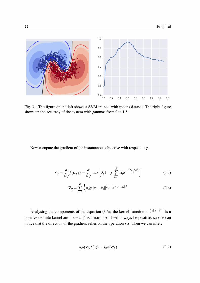
3.1 The figure on the left shows a SVM trained with moons dataset. The rightfigure shows up the accuracy of the system with gammas from 0 to 1.5. . . 22

3.2 Training progression of svm-GO applied in two datasets (a) Australian (b)German-numer, the three graphics shows (from left to right) the value ofgamma in each iteration, the system energy in each iteration, the number ofsupport vectors in each iteration. . . . . . . . . . . . . . . . . . . . . . . . 24

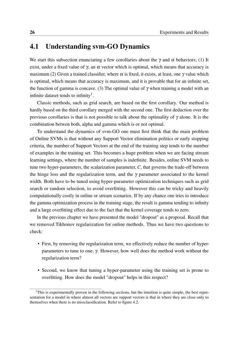
4.1 The subfigures below show three trained svm-GO with different dropoutvalues in both moons and blobs toy datasets, No dropout for figure (a)(d)40% for (b)(e) and 80% for (c)(f). One can observe how greater dropoutleads to a greater margin. . . . . . . . . . . . . . . . . . . . . . . . . . . . 27

xii List of figures

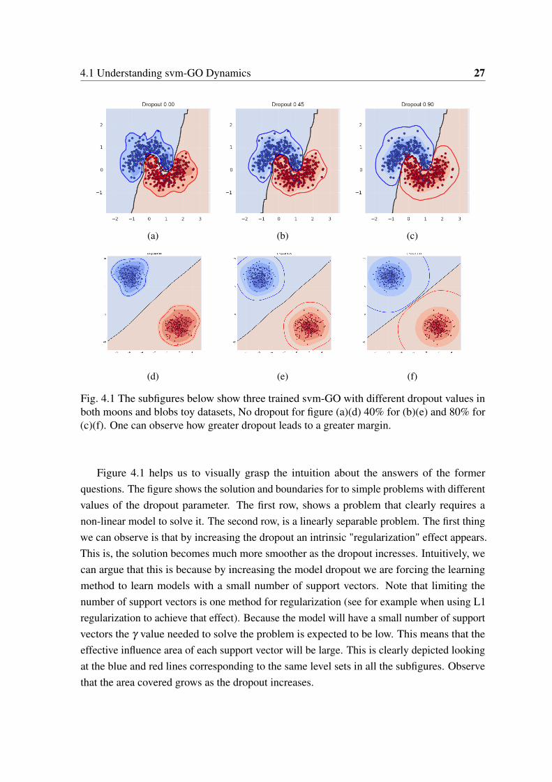
4.2 Gamma progress during the training step with different dropout values, sub-figure (a) belongs to german-numer dataset and sub-figure (b) belongs tosonar dataset. . . . . . . . . . . . . . . . . . . . . . . . . . . . . . . . . . 28

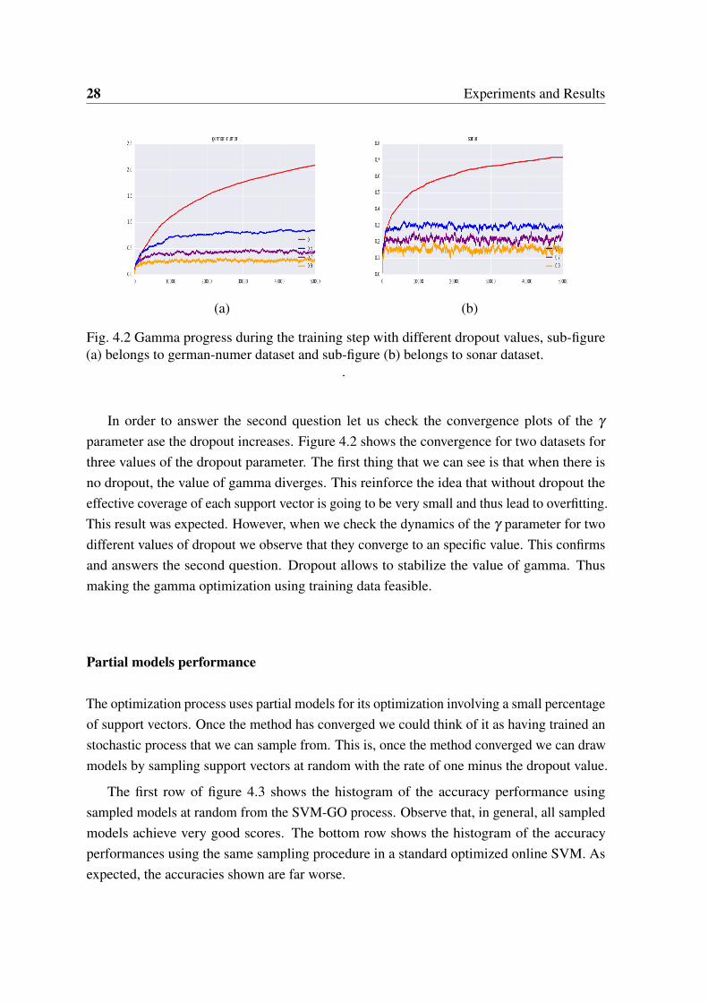
4.3 Histogram of the accuracy of the classifiers computed with a 20% of the totalSupport Vectors. The svm-GO model was trained using a dropout of 80%using sonar dataset. . . . . . . . . . . . . . . . . . . . . . . . . . . . . . . 29

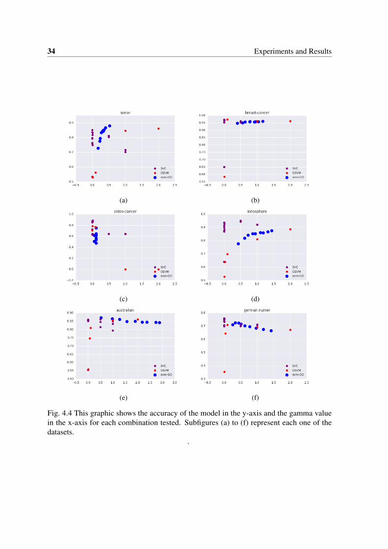
4.4 This graphic shows the accuracy of the model in the y-axis and the gammavalue in the x-axis for each combination tested. Subfigures (a) to (f) representeach one of the datasets. . . . . . . . . . . . . . . . . . . . . . . . . . . . 34

List of tables

4.1 Datasets . . . . . . . . . . . . . . . . . . . . . . . . . . . . . . . . . . . . 304.2 SVC Results . . . . . . . . . . . . . . . . . . . . . . . . . . . . . . . . . . 324.3 svm-GO Results . . . . . . . . . . . . . . . . . . . . . . . . . . . . . . . . 324.4 OSVM Results . . . . . . . . . . . . . . . . . . . . . . . . . . . . . . . . 324.5 Merged Results . . . . . . . . . . . . . . . . . . . . . . . . . . . . . . . . 33

Chapter 1

Introduction

1.1 Motivation

Support Vector Machines are a widely use model in Machine Learning (used for eitherclassification and regression), developed in the late 80’s. They appear as a result of thedevelopment of statistical learning framework, and its basis is a really intuitive concept.Given a dataset with samples corresponding to two different classes, find the hyperplane thatmaximizes the distance between both.

Of course, Support Vector Machines would be just another linear classifier without thekernel trick. This trick allows to replace any dot product by a function that satisfies specificconstraints. This implicitly generates a high dimensional space in which the method is ableto discriminate the classes in the datasets that are not linearly separable in the dimension ofthe original data.

On the other hand, from the beginning of this new millennium, Neural Networks haveregained large attention giving rise to the Deep Learning hype and its prosperity over thecommunity. Two are the main changes that allowed this technique to regain popularity,namely, the GPU’s based systems that allowed high computational capabilities and theincrease of the amount of data.

However, these two enablers are also some of the major limitations of this technique.Training a Deep Learning model is very expensive in terms of time, even with a goodinfrastructure. Also, there is a data limitation, the amount of data needed to train any DeepLearning system compared with all traditional methods is some orders of magnitude higherdue to the large classification capacity of the model. Besides, deep learning really shines inapplications where temporal or spacial correlations are found, namely, speech recognition,computer vision, or natural language processing, to name just a few.

2 Introduction

For all the reasons above, in front of classical record based, or attribute based data setssupport vector machines (SVM) are still the state of the art. This method also works well fordata exploration. Sometimes, in the industry one does not know how data "looks like", i.e. ifit is separable or not, if the number of features collected is enough, etc. In those cases a first(and cheap) approach may be a good starting point for a project.

These motivates us to improve the support vector machine model and try to make it aseasy to use as possible. In that way, this work tries to contribute to the community with theautomatic optimization of the hyper-parameters.

1.2 Goals

One of the drawbacks of using support vector machines is that one needs to fine tune manyhyper-parameters which are sensible to the data used to train the model. Here there is theobjective function of a Support Vector Machine with kernel:

f (α) =12||α||2 +C

N

∑i=1

max[0,1− yi

S

∑s=1

αsK(xi,xs,γ)]

where, C is the trade-off parameter for the regularization and optimization, and K(xi,xs,γ)

is some kernel function, xi are the training data points, xs are the support vectors, and γ

represents the hyper-parameters associated to the kernel function.

Usually, to train the best model, one does just do it by using grid search and crossvalidation on the hyper-parameters, validating with as many values as possible and keepingthe best one that leads to the best accuracy. This is not a cheap (in computational terms)job, and there are many combinations that lead to a provably good accuracy. Besides thecomputational inefficiency of the hyper-parameter optimization, there is not a good intuitionon what values should be tried.

The main focus of this work is to simplify the support vector machine by designinga technique able to automatically fine tune the hyper-parameters without cross-validationas well as to ease this tuning process as much as possible. In particular, we focus in theoptimization of γ parameter of a radial basis function (RBF) kernel in the online version ofsupport vector machines. The γ parameter regulates the influence area of a support vectorand has a high relevance in the final behaviour of the classifier.

1.3 Contributions 3

1.3 Contributions

The contributions of this work are the following:

• The formulation of the support vector machine is simplified to accommodate theconcept of model "dropout". This simplification allows to remove the regularizationterm without hindering the basic properties of the support vector machines. Thiseffectively removes the need of the C hyper-parameter.

• Model "dropout" is proposed and studied as a method to effectively and efficientlyallow the direct optimization of the γ hyper-parameter using training data (no validationdata is needed).

1.4 Outline

This work is distributed in five chapters. The first one, the current chapter, in which thedefinition of the problem and the motivations for this work are described, why we think thatthis research field is interesting, and the contributions to the community.

The second chapter focuses on the background theory to understand what are we tryingto work on; (1) we explain some basic concepts of statistical learning, the father of SVM’s.(2) The intuition about Support Vector Machines, starting by the definition of hyperplaneand optimal hyperplane, followed by the explanation of the primal and dual formulationwith some basic kernel theory and also the definition of Online SVM. (3) Related work thathas been done in model selection, all the methods and approaches used in Hyperparameteroptimization nowadays. There are currently three main approaches to face the model selectionproblem, one first approach using evolutionary algorithms, a probabilistic approach usingGaussian Processes and the third approach that uses gradient descent methods.

Chapter four contains the introduction and formulation of svm-GO, along all the sectionswe will explain the proposal of stochastic subgradient descent for optimizing gamma, and anouvelle regularization technique called model dropout which is a necessary condition forsvm-GO to work properly.

After the proposal, in the fifth chapter there’s first a deep explanation about the proposedmethod, svm-GO, and the expected dynamics. There are also a set of tables and figures withthe results of the experimental results that ground all the stated in the dynamics section.

Last we present the conclusion and the future lines of work.

Chapter 2

Background

2.1 Introduction

In this chapter we provide an introduction to the learning model based on [27] and the basicelements needed to understand all the concepts treated along this work. The first elementintroduced is statistical learning, which is the framework used for any learning model. Thenwe will jump into the derivation of Support Vector Machines and how the kernel trick can beapplied. The last section is about the related work in model selection field.

2.2 Statistical Learning

Statistical learning theory was introduced in the late 1960’s. In its basis it was a theoreticalanalysis of the problem of providing a function to define a given set of data. This theoryset the basis for Support Vector Machines, that where proposed in the early 1990’s. In thissection, the main concepts of statistical learning theory are explained.

The general learning model is defined by three main components: (1) A set of vectorsgenerated with an unknown distribution P(x), (2) A function that provides a vector y for eachprovided vector x according to the distribution P(y|x), (3) a learning machine that implementsa set of functions f (x,α) ∈ Λ. The problem lies in the way that the best function f (x,α) ∈ Λ

is selected [25].

The decision of selecting one or another function, in the function space Λ, is done based ina training set, which, ideally will contain a set of random independent identically distributedobservations describing the space α .

6 Background

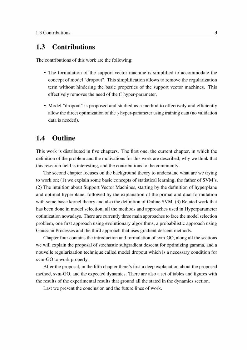
Fig. 2.1 An example of two classifiers (A, B) that separate green and blue circles.

Our final goal is to find the function f (x,α) which minimizes the risk functional:

R(α) =∫

L(y, f (x,α))dP(x,y) (2.1)

Where L(y, f (x,α)) is the loss function that measures the discrepancy between the realvalue y of x and the result of learning machine f (x,α). So in the end, the chosen functionf (x,α) is expected to be the one that better approximates the unknown distribution P(x).

2.2.1 Main learning problems

Despite the number of different problems in statistical learning is quite large, is possible toextrapolate three main categories of problems: Problems of pattern recognition, problems ofregression estimation and problems of density estimation.

Pattern Recognition This is probably the most common learning problem. Pattern Recog-nition problems are those which its output value can be either 0 or 1 y = {0,1}. Givenf (x,α),α ∈ Λ as the set of indicator functions, consider the following loss-function:

L(y, f (x,α)) =

{0 if y = f (x,α)

1 if y 6= f (x,α)(2.2)

In this scenario the problem is to find the indicator function that minimises the prob-ability of classification errors when the data is known, but the probability functionP(x,y) is unknown. The figure 2.1 shows an example of a classification problem.

2.2 Statistical Learning 7

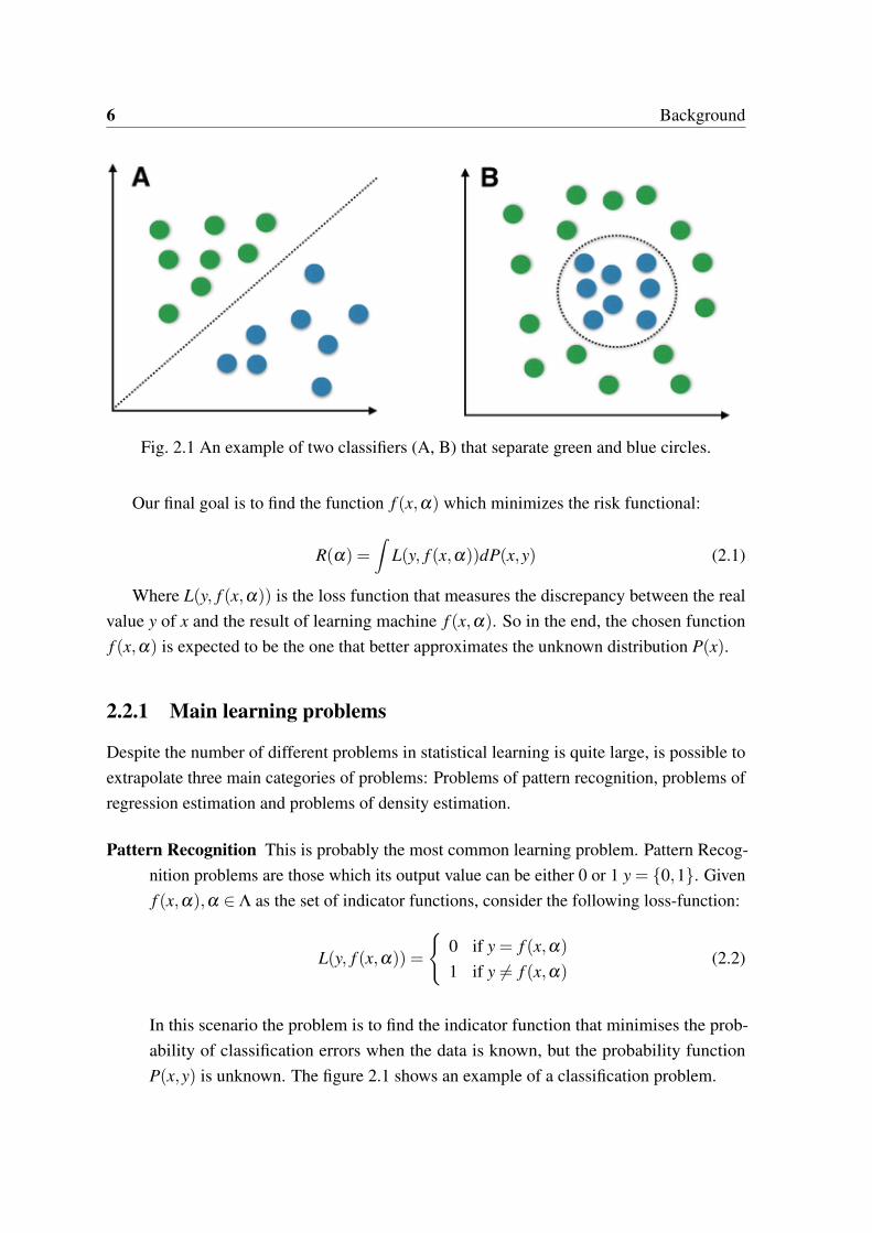
Fig. 2.2 Red points represents the data and the blue line is the regression function.

Regression Estimation In this case, the supervisor’s answer y is a real value and f (x,α),α ∈Λ the set of real functions that contains the regression function.

f (x,α) =∫

ydP(y|x) (2.3)

So, if the f (x,α) ∈ L2 the regression function is the one that minimizes the riskfunctional (2.1) with the following loss function:

L(y, f (x,α)) = (y− f (x,α))2 (2.4)

It can be said that the problem of regression estimation is the problem of minimizingthe risk functional (2.1) with the loss function (2.4) when the probability P(x,y) isunknown but the data is known. The figure 2.2 shows an example of the regressionproblem.

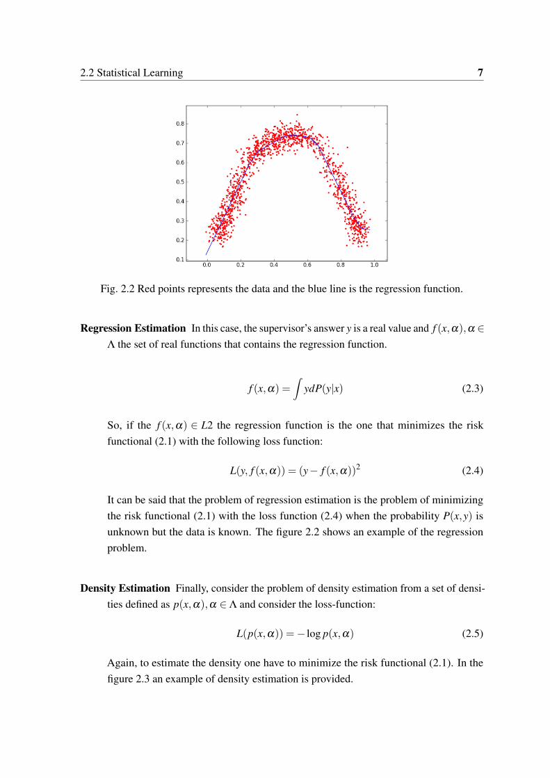
Density Estimation Finally, consider the problem of density estimation from a set of densi-ties defined as p(x,α),α ∈ Λ and consider the loss-function:

L(p(x,α)) =− log p(x,α) (2.5)

Again, to estimate the density one have to minimize the risk functional (2.1). In thefigure 2.3 an example of density estimation is provided.

8 Background

Fig. 2.3 An example of a density estimation problem

2.2.2 Empirical Risk Minimization

In a non-formal way, it is possible to explain the risk of a problem as the difference ofthe calculated distribution and the original distribution. Due to the fact that the originaldistribution is unknown, we need another measure in order to know how good is the calculateddistribution.

As it is said in the previous section, the learning problem is just a function estimationproblem [24]. To solve it one have to minimize the risk functional (2.1), but as the distributionP(x,y) it is unknown, this risk functional needs to be replaced by the empirical risk functional:

E(α) =1`

`

∑i=`

L(yi, f (xi,α) (2.6)

The induction principle of empirical risk minimization assumes that the function f (x,α)

which minimizes Remp(α) over the set α ∈ Λ results in a risk R(w∗`) close to its minimum.The soundness of the ERM principle needs to answer the two following questions [23]:

1. Does E(α) converges uniformly to the actual risk R(α) over the full set f (x,α),α ∈Λ?

2. What is the rate of convergence?

Thus nonasymptotic bounds of uniform convergence [26] are necessary to estimatethe quality of ERM method for a given sample size. VC dimension allows us to obtain aconstructive bound for the growth function.

The concepts of underfiting and overfitting appear when one wants to compare the originalfunction and the calculated function, as shown in Figure 2.4.

2.3 Support Vector Machines 9

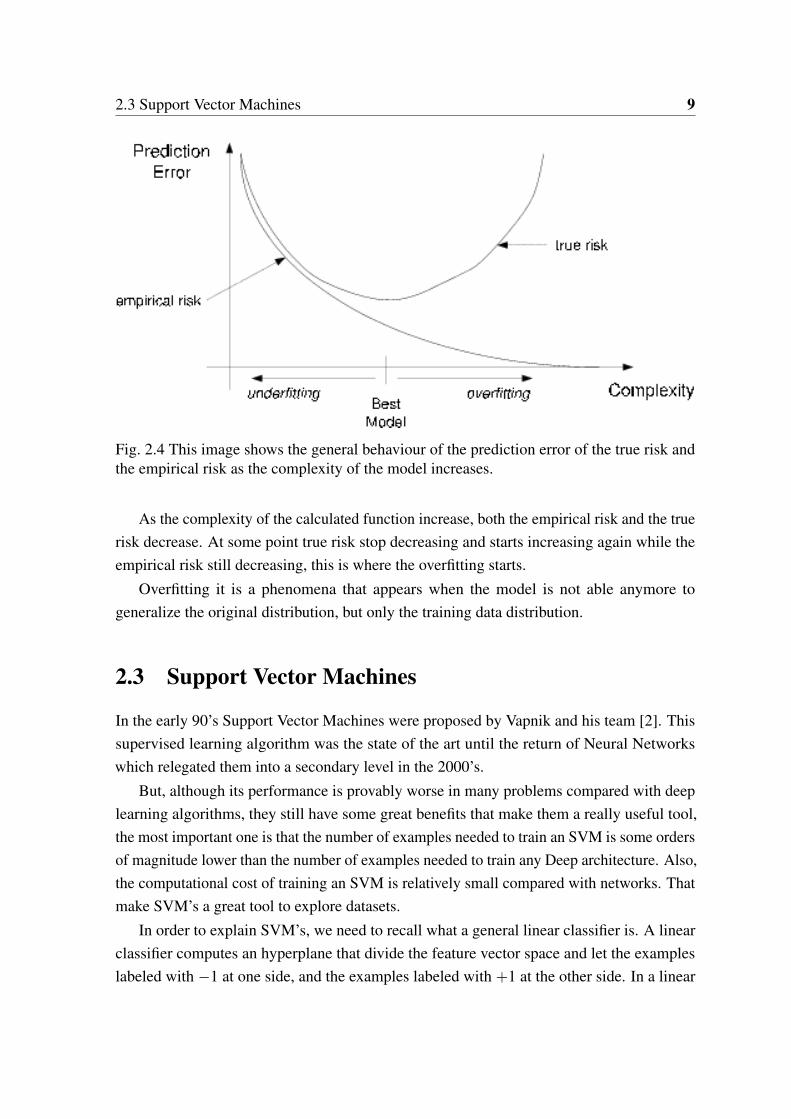
Fig. 2.4 This image shows the general behaviour of the prediction error of the true risk andthe empirical risk as the complexity of the model increases.

As the complexity of the calculated function increase, both the empirical risk and the truerisk decrease. At some point true risk stop decreasing and starts increasing again while theempirical risk still decreasing, this is where the overfitting starts.

Overfitting it is a phenomena that appears when the model is not able anymore togeneralize the original distribution, but only the training data distribution.

2.3 Support Vector Machines

In the early 90’s Support Vector Machines were proposed by Vapnik and his team [2]. Thissupervised learning algorithm was the state of the art until the return of Neural Networkswhich relegated them into a secondary level in the 2000’s.

But, although its performance is provably worse in many problems compared with deeplearning algorithms, they still have some great benefits that make them a really useful tool,the most important one is that the number of examples needed to train an SVM is some ordersof magnitude lower than the number of examples needed to train any Deep architecture. Also,the computational cost of training an SVM is relatively small compared with networks. Thatmake SVM’s a great tool to explore datasets.

In order to explain SVM’s, we need to recall what a general linear classifier is. A linearclassifier computes an hyperplane that divide the feature vector space and let the exampleslabeled with −1 at one side, and the examples labeled with +1 at the other side. In a linear

10 Background

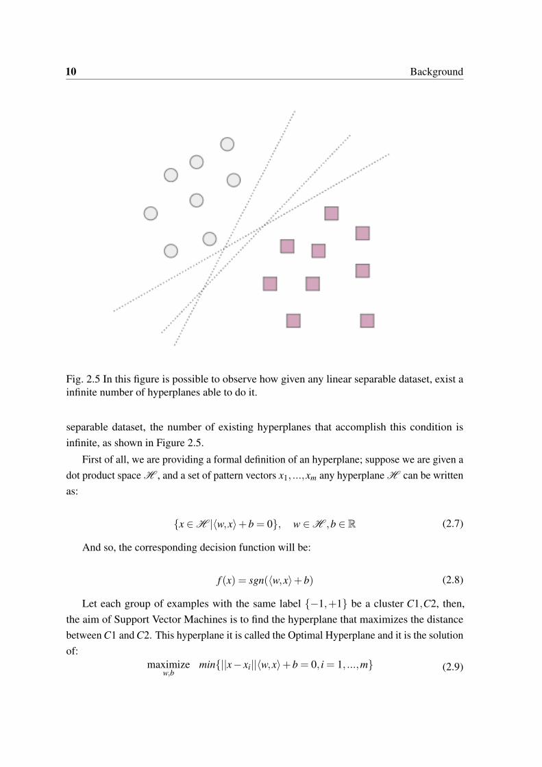
Fig. 2.5 In this figure is possible to observe how given any linear separable dataset, exist ainfinite number of hyperplanes able to do it.

separable dataset, the number of existing hyperplanes that accomplish this condition isinfinite, as shown in Figure 2.5.

First of all, we are providing a formal definition of an hyperplane; suppose we are given adot product space H , and a set of pattern vectors x1, ...,xm any hyperplane H can be writtenas:

{x ∈H |〈w,x〉+b = 0}, w ∈H ,b ∈ R (2.7)

And so, the corresponding decision function will be:

f (x) = sgn(〈w,x〉+b) (2.8)

Let each group of examples with the same label {−1,+1} be a cluster C1,C2, then,the aim of Support Vector Machines is to find the hyperplane that maximizes the distancebetween C1 and C2. This hyperplane it is called the Optimal Hyperplane and it is the solutionof:

maximizew,b

min{||x− xi||〈w,x〉+b = 0, i = 1, ...,m} (2.9)

2.3 Support Vector Machines 11

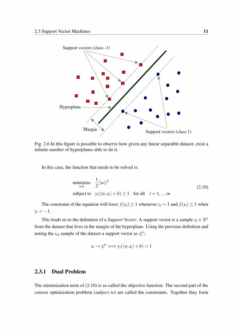
Fig. 2.6 In this figure is possible to observe how given any linear separable dataset, exist ainfinite number of hyperplanes able to do it.

In this case, the function that needs to be solved is:

minimizew,b

12||w||2

subject to yi(〈w,xi〉+b)≥ 1 for all i = 1, ...,m(2.10)

The constraint of the equation will force f (xi)≥ 1 whenever yi = 1 and f (xi)≤ 1 whenyi =−1.

This leads us to the definition of a Support Vector. A support vector is a sample xi ∈ Rn

from the dataset that lives in the margin of the hyperplane. Using the previous definition andnoting the ith sample of the dataset a support vector as xsv

i ;

xi→ xsvi ⇐⇒ yi(〈w,xi〉+b) = 1

2.3.1 Dual Problem

The minimization term of (2.10) is so called the objective function. The second part of theconvex optimization problem (subject to) are called the constraints. Together they form

12 Background

a constrained optimization problem, which can be dealt introducing Lagrange multipliersαi ≥ 0 and a Lagrangian:

L(w,b,α) =12||w||2−

m

∑i=1

αi(yi(〈xi,w〉+b)−1) (2.11)

The intuition lying above this formulation is that any time a constraint is violated, thenyi(〈xi,w〉+b)−1 < 0, in this case L can be increased by increasing the corresponding αi.At the same moment, w and b will need to change as long as L decreases.

According to the Karush-Kuhn-Tucker complementary conditions of optimization theorystatements, at the saddle point, the derivative of L respect to the primal variables must vanish.

∂

∂bL(w,b,α) = 0 and

∂

∂wL(w,b,α) = 0 (2.12)

which leads to:

m

∑i=1

αiyi = 0 (2.13)

And from the above formula, we can obtain:

w =m

∑i=1

αiyixi (2.14)

In this way, the dual formulation of SVM’s is obtained by removing the primal variablesin the Lagrangian.

maximizeα∈Rm

W (α) =m

∑i=1

αi−12

m

∑i, j=1

αiα jyiy j〈xi,x j〉

subject to αi ≥ 0∀ i = 1, ...,mm

∑i=1

αixi = 0

(2.15)

So, using the dual formulation, the hyperplane decision function is:

f (x) = sgn( m

∑i=1

αiyi〈x,xi〉+b)

(2.16)

All this formulations are valid, and provably work with any linear separable space. Thislinear separability is the ideal case, but of course, not the most common one (Figure 2.7).Working with non-separable linear dataset implies some slight modifications over our currentmodel.

2.3 Support Vector Machines 13

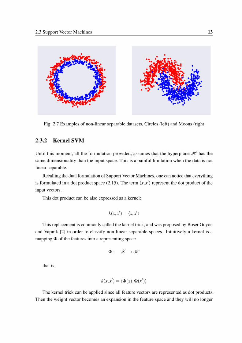
Fig. 2.7 Examples of non-linear separable datasets, Circles (left) and Moons (right

2.3.2 Kernel SVM

Until this moment, all the formulation provided, assumes that the hyperplane H has thesame dimensionality than the input space. This is a painful limitation when the data is notlinear separable.

Recalling the dual formulation of Support Vector Machines, one can notice that everythingis formulated in a dot product space (2.15). The term 〈x,x′〉 represent the dot product of theinput vectors.

This dot product can be also expressed as a kernel:

k(x,x′) = 〈x,x′〉

This replacement is commonly called the kernel trick, and was proposed by Boser Guyonand Vapnik [2] in order to classify non-linear separable spaces. Intuitively a kernel is amapping Φ of the features into a representing space

Φ : X →H

that is,

k(x,x′) = 〈Φ(x),Φ(x′)〉

The kernel trick can be applied since all feature vectors are represented as dot products.Then the weight vector becomes an expansion in the feature space and they will no longer

14 Background

correspond to the Φ-image of a single space input vector. Then the decision function is ofthe form

f (x) = sgn(m

∑i=1

yiαi〈Φ(x),Φ(x′)〉+b) (2.17)

and the quadratic program,

maximizeα∈Rm

W (α) =n

∑i=1

αi−12

m

∑i, j=1

αiα jyiy jk(xi,x j)

subject to αi ≥ 0 for all i = 1, ...,m, andm

∑i=1

αiyi = 0(2.18)

2.3.3 The RBF Kernel

Typically, when using support vector machines the default kernel is an RBF kernel. Thiskernel is widely used for this model with normalised datasets. A Radial Basis Functionkernel between two samples x,x′ ∈ Rn is defined as follows:

K(x,x′) = e−||x−x′||2

2σ2 (2.19)

This equation is defined in the range σ ∈ R\{0}. To avoid the undefined point whenσ = 0 we will substitute it by γ , using instead the equality γ = 1

σ2 , this results in the analogousequation:

K(x,x′) = e−γ||x−x′||2

2 (2.20)

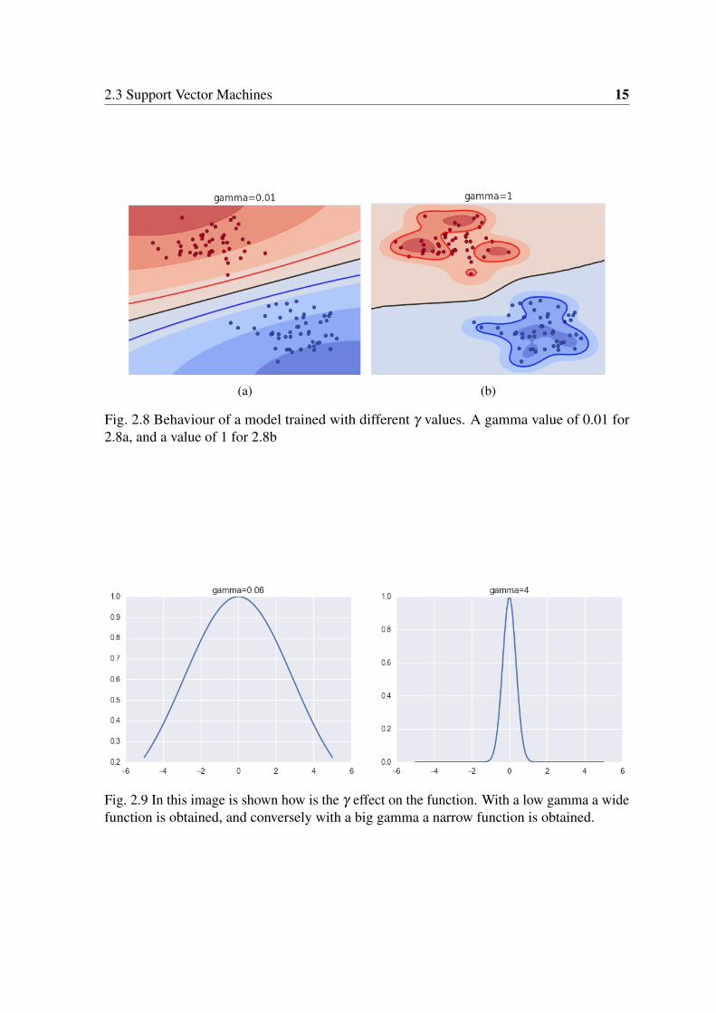
In terms of gamma, the bigger the gamma parameter is, the narrower the output, andthus the smaller the influence of each support vector affects its neighborhood. We can see inFigure 2.9. Recalling what stated in the discussion about Kernels, a narrow function means agreater distance between x and x′. Reconsidering the objective function of Support Vectormachines:

f (α) =12||α||2 +max

[0,1− yi

i

∑αie−γ||x−x′||2

2

](2.21)

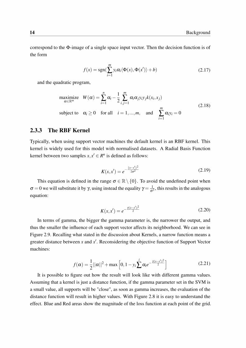
It is possible to figure out how the result will look like with different gamma values.Assuming that a kernel is just a distance function, if the gamma parameter set in the SVM isa small value, all supports will be "close", as soon as gamma increases, the evaluation of thedistance function will result in higher values. With Figure 2.8 it is easy to understand theeffect. Blue and Red areas show the magnitude of the loss function at each point of the grid.

2.3 Support Vector Machines 15

(a) (b)

Fig. 2.8 Behaviour of a model trained with different γ values. A gamma value of 0.01 for2.8a, and a value of 1 for 2.8b

Fig. 2.9 In this image is shown how is the γ effect on the function. With a low gamma a widefunction is obtained, and conversely with a big gamma a narrow function is obtained.

16 Background

2.3.4 Online SVM

All the formulation provided below assumes a batch training. This means that to train thealgorithm all the dataset is needed. This method has two important drawbacks; (1) As thedataset size increases, the computational resources in needed to train the model in batchmode also increase. So dealing with large datasets can become a big problem. (2) Once themodel is trained, if one wants to update it with new incoming data, the process has to startagain.

In that conext appeared online methods, taking advantage of the primal decomposition ofthe kernel formulation. Online methods are related to stochastic gradient methods becausethey operate with one example at the time. All online methods are based on the idea belowPerceptron[20], which was the first online learner, It works cycling repeatedly through thepatterns they update the internal state stored in the weight vector when a condition is satisfied.Perceptron can be seen as implementing a stochastic gradient step. Nevertheless, onlinelearning algorithms were proposed as fast alternatives to SVMs.

The first algorithm to merge the idea below perceptron with SVM was the so-calledvoted-perceptron [7]. After it, first NORMA [13] and some years later Pegasos [21] tookthe flagship of online versions of Support Vector Machines. All this algorithms take advan-tage of Stochastic Subgradient Methods, as mentioned below, and are proven to convergeasymptotically to the correct solution.

2.4 Related Work 17

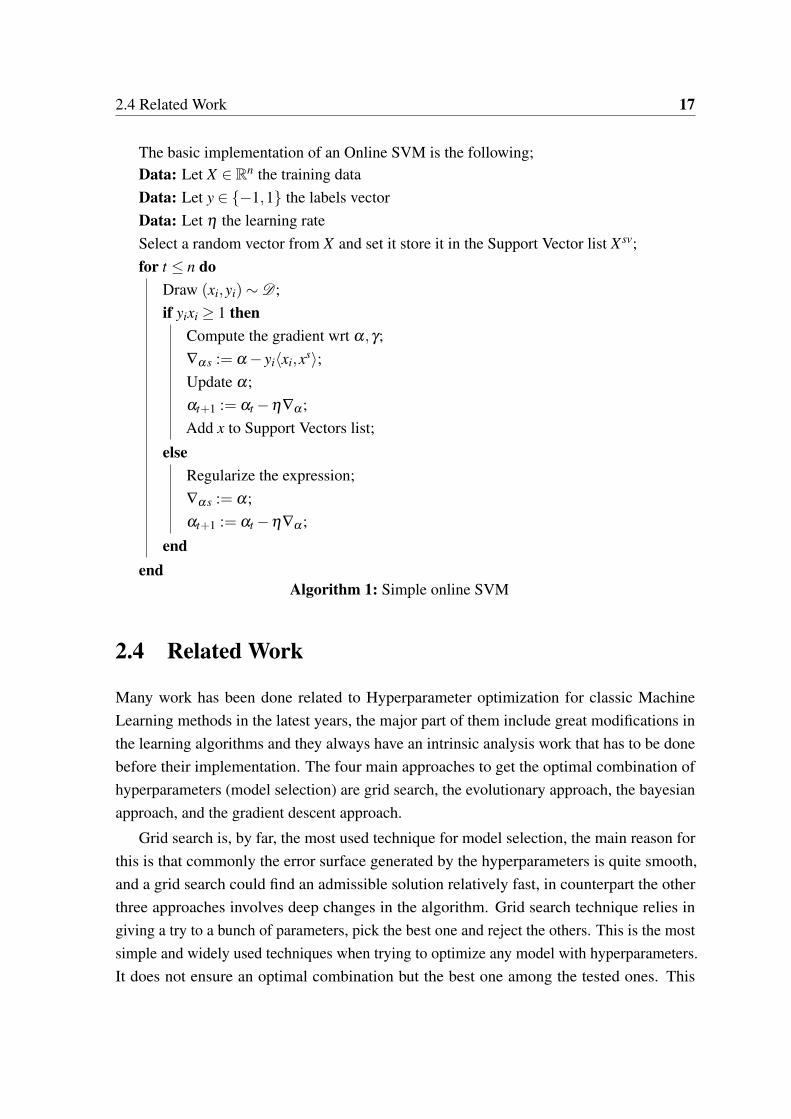
The basic implementation of an Online SVM is the following;Data: Let X ∈ Rn the training dataData: Let y ∈ {−1,1} the labels vectorData: Let η the learning rateSelect a random vector from X and set it store it in the Support Vector list X sv;for t ≤ n do

Draw (xi,yi)∼D ;if yixi ≥ 1 then

Compute the gradient wrt α,γ;∇α s := α− yi〈xi,xs〉;Update α;αt+1 := αt−η∇α ;Add x to Support Vectors list;

elseRegularize the expression;∇α s := α;αt+1 := αt−η∇α ;

endend

Algorithm 1: Simple online SVM

2.4 Related Work

Many work has been done related to Hyperparameter optimization for classic MachineLearning methods in the latest years, the major part of them include great modifications inthe learning algorithms and they always have an intrinsic analysis work that has to be donebefore their implementation. The four main approaches to get the optimal combination ofhyperparameters (model selection) are grid search, the evolutionary approach, the bayesianapproach, and the gradient descent approach.

Grid search is, by far, the most used technique for model selection, the main reason forthis is that commonly the error surface generated by the hyperparameters is quite smooth,and a grid search could find an admissible solution relatively fast, in counterpart the otherthree approaches involves deep changes in the algorithm. Grid search technique relies ingiving a try to a bunch of parameters, pick the best one and reject the others. This is the mostsimple and widely used techniques when trying to optimize any model with hyperparameters.It does not ensure an optimal combination but the best one among the tested ones. This

18 Background

search can be as exhaustive as the user wants, but usually it is enough with a 5x5 grid thatleads up to 25 experiments. This is simple but unefficient.

In the branch of evolutionary approaches there are [8][15], their method is based in thecovariance matrix adaptation evolution strategy and is used to determine the kernel from aparameterized kernel space and to control the regularization. Their method is applicable tooptimize non-differentiable kernel functions and arbitrary model selection criteria. In [14]they propose a strategy using genetic algorithms to learn combined kernels in a data-drivenmanner and to determine all free kernel parameters.

The Bayesian approach stands on a Gaussian Process that models the learning algorithmsgeneralization performance. The tractable posterior distribution induced by the GaussianProcess leads to efficient use of the information gathered by previous experiments [22]. Forthe Support Vector Machine case there are many approaches [30][28][29] based on the initialimplementation of [19] and posterior extended to the non-linear case.

There are some approaches that use gradient descent as a guide to find a local minima ofthe parameters that allow the model to generalize the best [3], in [5][11] they use the radiusmargin (RM) using L2 to approximate the best C and γ . In [9] a model selection strategyusing the span of support vectors is proposed. All the methods mentioned have the drawbackthat the kernel function needs to be differentiable in order to be able to compute the gradient.

Both the probabilistic approach using Gaussian Processes, and the evolutionary approachadd an extra complexity to the algorithm. Using Hidden Markov Models, even it is proven toperform well, does not do much in favour of the explainability of the data. And evolutionaryalgorithms require an expensive pre-training phase. In addition, all techniques mentionedbefore aims to generalise the optimization to any kind of kernel. Our approach, svm-GO,is based on gradient descent techniques, more concretely, it uses Stochastic SubgradientDescent (SSGD) and it is focused on RBF kernel and removes both C and γ parameters. Thekeypoint of our algorithm is the simplicity, one must tune only one parameter (the dropout)in order to make it work.

Chapter 3

Proposal

So after introducing all the background relative to Statistical Learning and how SupportVector Machine model is derived from it, this section is devoted to define how, using kerneltheory and coordinate descent, the kernel hyperparameters can be automatically optimized.

Hyperparameters, in machine learning, are those parameters that are set "a priori", not bytraining, usually using a validation set. In learning models the most common way to tune thehyperparameters is using grid search. This heuristic method consists in training the modelwith many parameter combinations and pick the one that best fit the introduced data.

This procedure is really inefficient due to the fact that, commonly, the number of com-binations to test is large, and even with an exhaustive search one cannot determine that thecombination found is the optimal one.

The main goal of this work is to present a method which is able to automatically tunethe hyperparameters of a kernel in an online implementation of the Support Vector Machineusing Stochastic Sub-Gradient Descent (SSGD). Before going into the method proposal it isimportant to state that in the traditional Support Vector Machine setting the joint optimizationof gamma and weight values will lead to overfitting. There is a strong reason for this, noticethat if the minimiser works with all the training set, the optimal value for gamma will alwaystend to ∞. This happens because the minimisation function in terms of γ is an increasingmonotone function.

In this work we take advantage of training using stochastic subgradient methods tooverpass this effect. The intuition behind the method is that the training set under the learnerperception changes at each iteration, and by computing the gradient of γ with a part of themodel is possible to obtain a decent representation. But even with SSGD optimisation, thereis a great risk of overfitting.

To bypass (or, at least delay) the overfitting effect, we have developed a dropout methodinspired on Deep Learning framework. Even that is far from being technically the same

20 Proposal

concept, in the theoretical context works really similar. The main idea is to use a differentsubset of support vectors sampled from the support vector set according to a “dropout”parameter at each iteration of the optimization process. In this sense, at each iteration, weare minimizing the objective function considering a different model. The hypothesis is thatby doing this the gamma parameter can not specifically focus on the training data and thuseffectively delay overfitting while tuning the gamma parameter.

We call this method model dropout. The reason for this name is because by focusing ona subsampled set of support vectors, we are effectively changing the model selected.

3.1 Model dropout for gamma optimization

All this work is devoted to explore if it is possible to automatically optimize the parameter γ .But, what does one understand by the optimal value? The optimal value of γ is that one withwhich the higher score is obtained in test evaluation. Or, analogously, the value with whichthe loss function gets the smallest accumulated addition.

In order to provide a basis for the previous statement let v1, ...,vi ∈ Rn, i ∈ N the featurevectors, and v′1, ...,v

′j ∈ Rn, j ∈ N the support vectors of a trained Support Vector Machine.

It exists a value of γ > 0,γ ∈ R which maximise the accuracy of the classifier using theclassical formulation of Support Vector Machines, and even it is not a completely-convexfunction, it has single maximum.

The results shown in figure 3.1 endorse the previous affirmation. The system was trainedusing online Support Vector Machine and the scores were obtained using test data. Ourformulation simplifies the original SVM. In this case we drop the regularization term. Thereason behind this decision is that we want to clearly study the effect of the model dropoutwithout the influences of the regularization term. In this sense, we hypothesize and we willconfirm that the model dropout works as a “regularizer” in terms of combating overfitting.

Then the objective function turns into:

f (x) =N

∑i=1

max[0,1− yi

S

∑s=1

αse−12 γ||xi−xs||2

](3.1)

Where αs is the subset of alphas corresponding to the S support vectors, xs the supportvectors samples and xi the training data samples.

And the decision function is:

h(x) = sgnS

∑s=1

(αse−

12 γ||x−xs||2

)(3.2)

3.1 Model dropout for gamma optimization 21

where xs corresponds to each of the S support vectors, and αs is the support vector weight.

This algorithm is prone to failure in a deterministic setting. For this proposal to besuccessful we have to change to an stochastic setting. In the stochastic setting the objectivefunction shown before becomes a variational upper bound of the expected loss function[16].To explain the variational bound let ζn = `− yn(wT x̃) so the expected hinge loss over thedata distribution D can be written as the objective of the following optimization problem:

minimize ED [max(0,ζn)] (3.3)

Let us now define an stochastic process of order k, PD(k), as the random process onall support vector models over a data distribution D with k support vectors. This is, leth(x) be a random sample of the stochastic process PD(k), i.e. h(x)∼PD(k) then h(x) isa support vector machine model with exactly k support vectors. Observe that we can drawmany different random models with exactly k support vectors.

The proposed model is to change the equation 3.3 to accommodate the stochastic process,so that the problem to optimize becomes

minimize EP(k),D [max(0,ζn)] (3.4)

Observe, that this formulation considers the expected value over the data distribution andthe stochastic model process of order k.

In practice, we can reduce this objective to the partial optimization of the hinge loss givena sample from the data set and a sample from the stochastic process of order k. This is, ateach iteration of the optimization algorithm we sample the data set and the process and adjustthe parameters according to those particular samples.

In order to sample the stochastic process suffices to randomly select a subset of k supportvectors. This mechanism resembles that of dropout in neural networks[4]. However, insteadof setting random sample attributes in the data set to zero, we set to zero all support vectorsexcept for the k selected in that iteration. For this reason we called this process modeldropout.

In order to solve this problem, we will use stochastic subgradient methods. Thus we haveto derive the gradients with respect to the parameters to optimize, i.e. γ and α . However, inthe stochastic setting this is done with respect to an instantaneous loss function, i.e. the hingeloss for one sample and a single model of order k,

max(0,1− yi

K

∑s=1

αse−12 γ‖xi−xs‖2

)

22 Proposal

Fig. 3.1 The figure on the left shows a SVM trained with moons dataset. The right figureshows up the accuracy of the system with gammas from 0 to 1.5.

Now compute the gradient of the instantanous objective with respect to γ :

∇γ =∂

∂γf (α,γ) =

∂

∂γmax

[0,1− yi

K

∑s=1

αse−γ||xi−xs||2

2

](3.5)

∇γ =K

∑s=1

12

αsy||xi− xs||2e−12 γ||xi−xs||2 (3.6)

Analysing the components of the equation (3.6); the kernel function e−12 γ||x−x′||2 is a

positive definite kernel and ||x− x′||2 is a norm, so it will always be positive, so one cannotice that the direction of the gradient relies on the operation yα . Then we can infer:

sgn(∇γ f (x)) = sgn(αy) (3.7)

3.1 Model dropout for gamma optimization 23

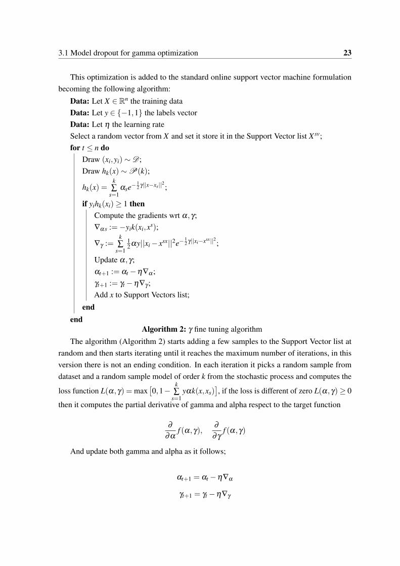
This optimization is added to the standard online support vector machine formulationbecoming the following algorithm:

Data: Let X ∈ Rn the training dataData: Let y ∈ {−1,1} the labels vectorData: Let η the learning rateSelect a random vector from X and set it store it in the Support Vector list X sv;for t ≤ n do

Draw (xi,yi)∼D ;Draw hk(x)∼P(k);

hk(x) =k∑

s=1αse−

12 γ||x−xs||2;

if yihk(xi)≥ 1 thenCompute the gradients wrt α,γ;∇α s :=−yik(xi,xs);

∇γ :=k∑

s=1

12αy||xi− xsx||2e−

12 γ||xi−xsx||2;

Update α,γ;αt+1 := αt−η∇α ;γt+1 := γt−η∇γ ;Add x to Support Vectors list;

endend

Algorithm 2: γ fine tuning algorithm

The algorithm (Algorithm 2) starts adding a few samples to the Support Vector list atrandom and then starts iterating until it reaches the maximum number of iterations, in thisversion there is not an ending condition. In each iteration it picks a random sample fromdataset and a random sample model of order k from the stochastic process and computes the

loss function L(α,γ) = max[0,1−

k∑

s=1yαk(x,xs)

], if the loss is different of zero L(α,γ)≥ 0

then it computes the partial derivative of gamma and alpha respect to the target function

∂

∂αf (α,γ),

∂

∂γf (α,γ)

And update both gamma and alpha as it follows;

αt+1 = αt−η∇α

γt+1 = γt−η∇γ

24 Proposal

Then it adds the randomly chosen vector into the support vector list xsv← x. If the lossfunction returns a zero L(α.γ) = 0 then it means that the vector is correctly classified.

For the sake of simplicity we can use a surrogate parameter to the order k, this is thedropout parameter κ . The relationship between both is κ = k

N . Working with κ is easierbecause the parameter is bounded between 0 and 1.

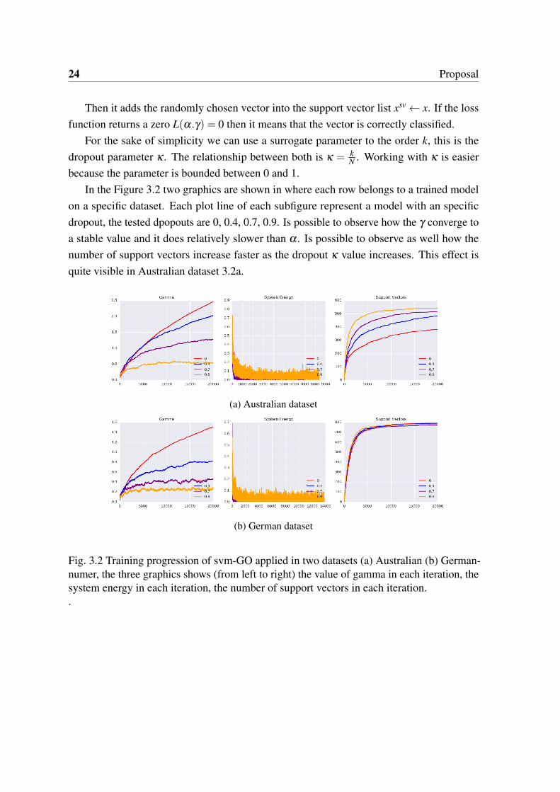
In the Figure 3.2 two graphics are shown in where each row belongs to a trained modelon a specific dataset. Each plot line of each subfigure represent a model with an specificdropout, the tested dpopouts are 0, 0.4, 0.7, 0.9. Is possible to observe how the γ converge toa stable value and it does relatively slower than α . Is possible to observe as well how thenumber of support vectors increase faster as the dropout κ value increases. This effect isquite visible in Australian dataset 3.2a.

(a) Australian dataset

(b) German dataset

Fig. 3.2 Training progression of svm-GO applied in two datasets (a) Australian (b) German-numer, the three graphics shows (from left to right) the value of gamma in each iteration, thesystem energy in each iteration, the number of support vectors in each iteration..

Chapter 4

Experiments and Results

This chapter is devoted to the explanation of the experimental results obtained with gammaoptimization. All the experiments have been performed using ten UCI datasets that will belisted and described in the following sections. Over this chapter we will show, in the first part,the intuition about the method. Why it works with dropout, and why Thikonov regularizationis no longer needed. Then, the method is compared with online svm and standard batch svmin terms of performance metrics.

The model with gamma optimization is a custom implementation based on the basiconline SVM. We have removed all noisy components and all boosters that could interferewith our method in order to be able to clearly explain how the system behaves.

Before going deeper in the method dynamics description, the experimentation method-ology that has been followed in order to allow a fair comparison among the methods is asfollows: First, the same train an test sets splits for all experiments are used. Also, in order toreduce the stochastic component that this model contains, we have defined a seed to forcea predefined selection order of samples for the stochastic subgradient method. Recall thatin each iteration of the algorithm a random sample is picked from the dataset. Using a seedallows us to ensure that the vectors are picked in the same order in all experiments and thusthat no sample selection bias is present. In addition, we have tested the method against thebatch implementation of the Support Vector Machine included in the python package sklearn.Contrary to the online methods, batch SVM has access to the full data set for its optimization,as such the results achieved by this method have to be considered as the goal to be achieved.We use grid-search for hyperparameter optimization with Tikhonov regularization.

26 Experiments and Results

4.1 Understanding svm-GO Dynamics

We start this subsection enunciating a few corollaries about the γ and α behaviors; (1) Itexist, under a fixed value of γ , an α vector which is optimal, which means that accuracy ismaximum (2) Given a trained classifier, where α is fixed, it exists, at least, one γ value whichis optimal, which means that accuracy is maximum, and it is provable that for an infinite set,the function of gamma is concave. (3) The optimal value of γ when training a model with aninfinite dataset tends to infinity1.

Classic methods, such as grid search, are based on the first corollary. Our method ishardly based on the third corollary merged with the second one. The first deduction over theprevious corollaries is that is not possible to talk about the optimality of γ alone. It is thecombination betwen both, alpha and gamma which is or not optimal.

To understand the dynamics of svm-GO one must first think that the main problemof Online SVMs is that without any Support Vector elimination politics or early stoppingcriteria, the number of Support Vectors at the end of the training step tends to the numberof examples in the training set. This becomes a huge problem when we are facing streamlearning settings, where the number of samples is indefinite. Besides, online SVM needs totune two hyper-parameters, the scalarization parameter, C, that governs the trade-off betweenthe hinge loss and the regularization term, and the γ parameter associated to the kernelwidth. Both have to be tuned using hyper-parameter optimization techniques such as gridsearch or random selection, to avoid overfitting. However this can be tricky and heavilycomputationally costly in online or stream scenarios. If by any chance one tries to introducethe gamma optimization process in the training stage, the result is gamma tending to infinityand a large overfitting effect due to the fact that the kernel coverage tends to zero.

In the previous chapter we have presented the model "dropout" as a proposal. Recall thatwe removed Tikhonov regularization for online methods. Thus we have two questions tocheck:

• First, by removing the regularization term, we effectively reduce the number of hyper-parameters to tune to one, γ . However, how well does the method work without theregularization term?

• Second, we know that tuning a hyper-parameter using the training set is prone tooverfitting. How does the model "dropout" helps in this respect?

1This is experimentally proven in the following sections, but the intuition is quite simple, the best repre-sentation for a model in where almost all vectors are support vectors is that in where they are close only tothemselves when there is no missclassification. Refer to figure 4.2.

4.1 Understanding svm-GO Dynamics 27

(a) (b) (c)

(d) (e) (f)

Fig. 4.1 The subfigures below show three trained svm-GO with different dropout values inboth moons and blobs toy datasets, No dropout for figure (a)(d) 40% for (b)(e) and 80% for(c)(f). One can observe how greater dropout leads to a greater margin.

Figure 4.1 helps us to visually grasp the intuition about the answers of the formerquestions. The figure shows the solution and boundaries for to simple problems with differentvalues of the dropout parameter. The first row, shows a problem that clearly requires anon-linear model to solve it. The second row, is a linearly separable problem. The first thingwe can observe is that by increasing the dropout an intrinsic "regularization" effect appears.This is, the solution becomes much more smoother as the dropout incresses. Intuitively, wecan argue that this is because by increasing the model dropout we are forcing the learningmethod to learn models with a small number of support vectors. Note that limiting thenumber of support vectors is one method for regularization (see for example when using L1regularization to achieve that effect). Because the model will have a small number of supportvectors the γ value needed to solve the problem is expected to be low. This means that theeffective influence area of each support vector will be large. This is clearly depicted lookingat the blue and red lines corresponding to the same level sets in all the subfigures. Observethat the area covered grows as the dropout increases.

28 Experiments and Results

(a) (b)

Fig. 4.2 Gamma progress during the training step with different dropout values, sub-figure(a) belongs to german-numer dataset and sub-figure (b) belongs to sonar dataset.

.

In order to answer the second question let us check the convergence plots of the γ

parameter ase the dropout increases. Figure 4.2 shows the convergence for two datasets forthree values of the dropout parameter. The first thing that we can see is that when there isno dropout, the value of gamma diverges. This reinforce the idea that without dropout theeffective coverage of each support vector is going to be very small and thus lead to overfitting.This result was expected. However, when we check the dynamics of the γ parameter for twodifferent values of dropout we observe that they converge to an specific value. This confirmsand answers the second question. Dropout allows to stabilize the value of gamma. Thusmaking the gamma optimization using training data feasible.

Partial models performance

The optimization process uses partial models for its optimization involving a small percentageof support vectors. Once the method has converged we could think of it as having trained anstochastic process that we can sample from. This is, once the method converged we can drawmodels by sampling support vectors at random with the rate of one minus the dropout value.

The first row of figure 4.3 shows the histogram of the accuracy performance usingsampled models at random from the SVM-GO process. Observe that, in general, all sampledmodels achieve very good scores. The bottom row shows the histogram of the accuracyperformances using the same sampling procedure in a standard optimized online SVM. Asexpected, the accuracies shown are far worse.

4.2 Results 29

(a)

(b)

Fig. 4.3 Histogram of the accuracy of the classifiers computed with a 20% of the total SupportVectors. The svm-GO model was trained using a dropout of 80% using sonar dataset..

4.2 Results

In this results sections we compare svm-GO against svm online and SVC methods to showthe performance of our method, in the following subsections we will detail the datasets used,a detailed view of the techniques and the parameter setting to allow anyone to reproduce theshown results.

30 Experiments and Results

Table 4.1 Datasets

Instances Features Classes Class1 Instances Class2 Instancesphishing 11055 68 2 4898 (44%) 6157 (55%)splice 1000 60 2 483 (48%) 517 (51%)ionosphere 351 34 2 126 (35%) 225 (64%)diabetes 768 8 2 268 (34%) 500 (65%)german-numer 1000 24 2 700 (70%) 300 (30%)sonar 208 60 2 111 (53%) 97 (46%)svmguide1 3089 4 2 1089 (35%) 2000 (64%)australian 690 14 2 383 (55%) 307 (44%)breast-cancer 683 10 2 444 (65%) 239 (34%)colon-cancer 62 2000 2 40 (64%) 22 (35%)

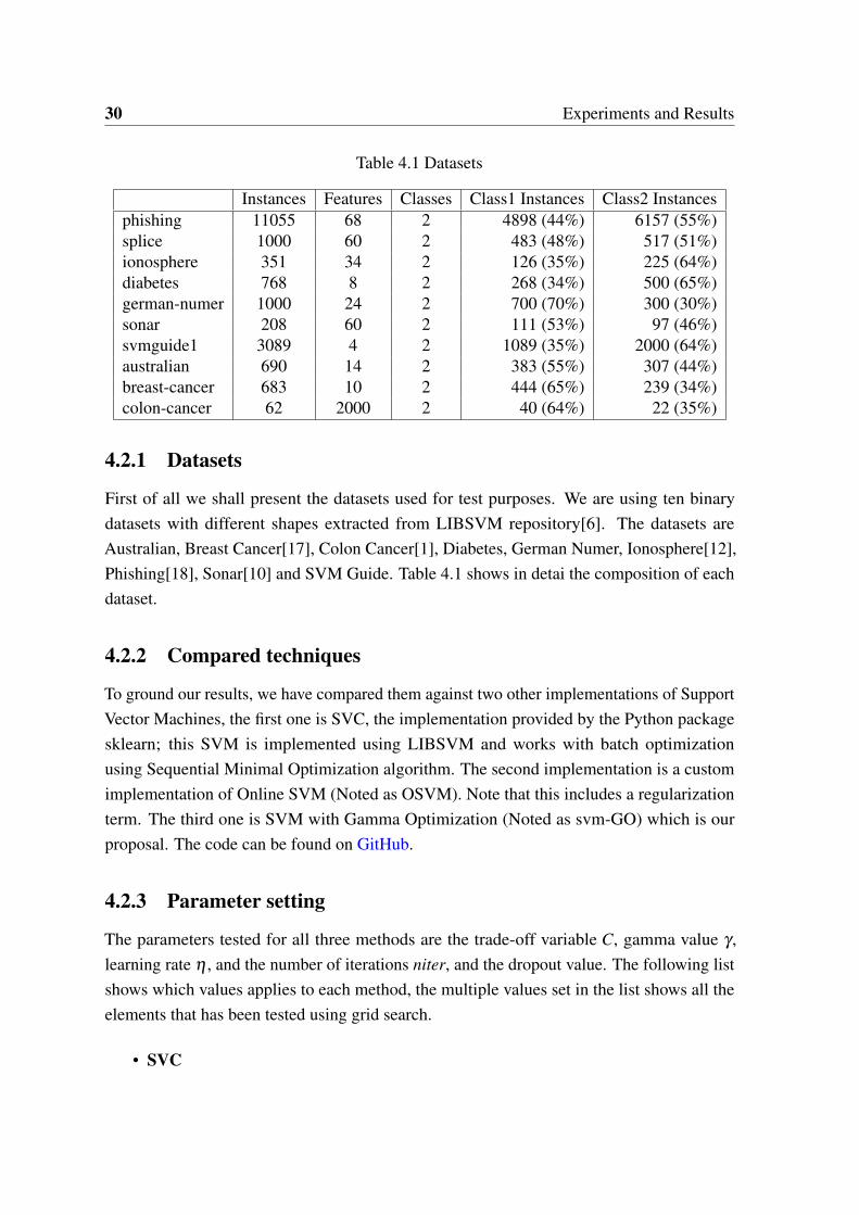
4.2.1 Datasets

First of all we shall present the datasets used for test purposes. We are using ten binarydatasets with different shapes extracted from LIBSVM repository[6]. The datasets areAustralian, Breast Cancer[17], Colon Cancer[1], Diabetes, German Numer, Ionosphere[12],Phishing[18], Sonar[10] and SVM Guide. Table 4.1 shows in detai the composition of eachdataset.

4.2.2 Compared techniques

To ground our results, we have compared them against two other implementations of SupportVector Machines, the first one is SVC, the implementation provided by the Python packagesklearn; this SVM is implemented using LIBSVM and works with batch optimizationusing Sequential Minimal Optimization algorithm. The second implementation is a customimplementation of Online SVM (Noted as OSVM). Note that this includes a regularizationterm. The third one is SVM with Gamma Optimization (Noted as svm-GO) which is ourproposal. The code can be found on GitHub.

4.2.3 Parameter setting

The parameters tested for all three methods are the trade-off variable C, gamma value γ ,learning rate η , and the number of iterations niter, and the dropout value. The following listshows which values applies to each method, the multiple values set in the list shows all theelements that has been tested using grid search.

• SVC

4.2 Results 31

– C: [1, 10, 100]

– γ: [1, 0.5, ’auto’2, 1e-2, 1e-3, 1e-4, 1e-5]

• OSVM

– η : 0.01

– niter: 30.000

– γ: [2, 1, 0.5, ’auto’, 1e-2]

• svm-GO

– η : 0.01

– niter: 30.000

– dropout: [0.1, 0.2, 0.3, 0.4, 0.5, 0.6, 0.7, 0.8, 0.9]

4.2.4 Experimental results

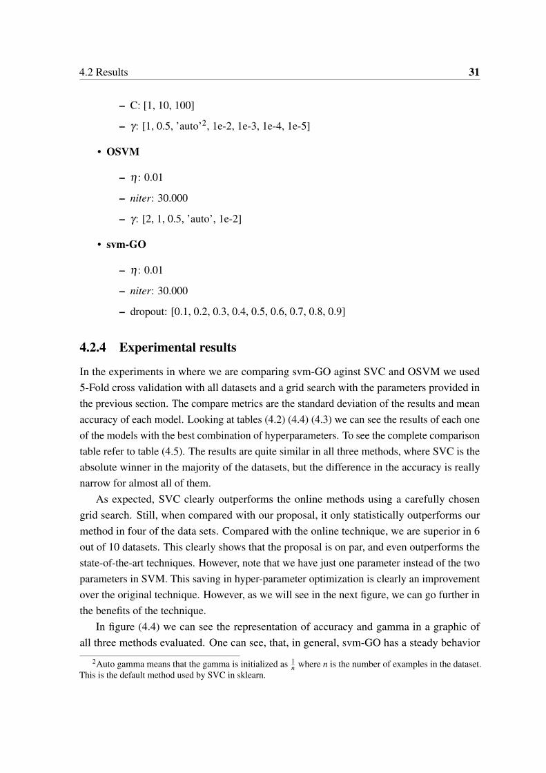
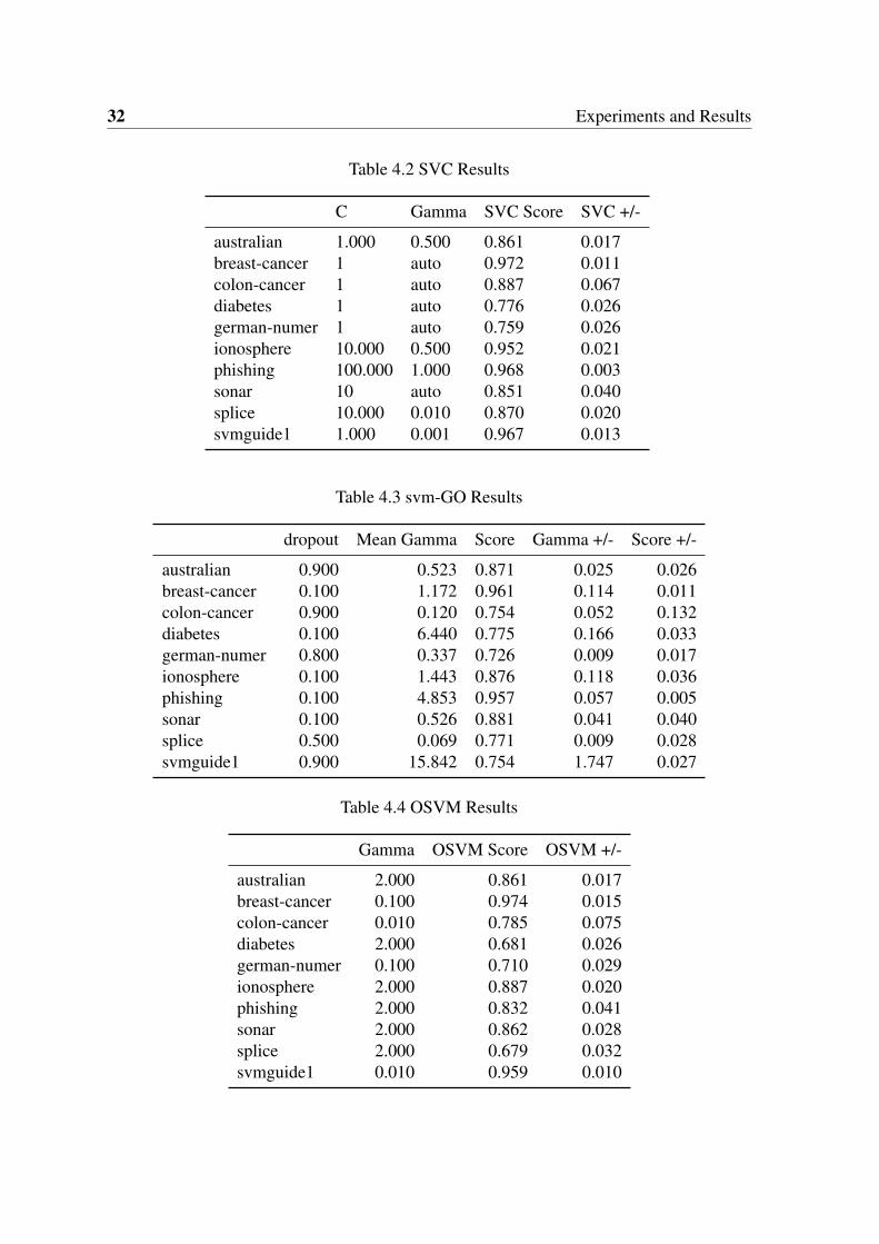
In the experiments in where we are comparing svm-GO aginst SVC and OSVM we used5-Fold cross validation with all datasets and a grid search with the parameters provided inthe previous section. The compare metrics are the standard deviation of the results and meanaccuracy of each model. Looking at tables (4.2) (4.4) (4.3) we can see the results of each oneof the models with the best combination of hyperparameters. To see the complete comparisontable refer to table (4.5). The results are quite similar in all three methods, where SVC is theabsolute winner in the majority of the datasets, but the difference in the accuracy is reallynarrow for almost all of them.

As expected, SVC clearly outperforms the online methods using a carefully chosengrid search. Still, when compared with our proposal, it only statistically outperforms ourmethod in four of the data sets. Compared with the online technique, we are superior in 6out of 10 datasets. This clearly shows that the proposal is on par, and even outperforms thestate-of-the-art techniques. However, note that we have just one parameter instead of the twoparameters in SVM. This saving in hyper-parameter optimization is clearly an improvementover the original technique. However, as we will see in the next figure, we can go further inthe benefits of the technique.

In figure (4.4) we can see the representation of accuracy and gamma in a graphic ofall three methods evaluated. One can see, that, in general, svm-GO has a steady behavior

2Auto gamma means that the gamma is initialized as 1n where n is the number of examples in the dataset.

This is the default method used by SVC in sklearn.

32 Experiments and Results

Table 4.2 SVC Results

C Gamma SVC Score SVC +/-

australian 1.000 0.500 0.861 0.017breast-cancer 1 auto 0.972 0.011colon-cancer 1 auto 0.887 0.067diabetes 1 auto 0.776 0.026german-numer 1 auto 0.759 0.026ionosphere 10.000 0.500 0.952 0.021phishing 100.000 1.000 0.968 0.003sonar 10 auto 0.851 0.040splice 10.000 0.010 0.870 0.020svmguide1 1.000 0.001 0.967 0.013

Table 4.3 svm-GO Results

dropout Mean Gamma Score Gamma +/- Score +/-

australian 0.900 0.523 0.871 0.025 0.026breast-cancer 0.100 1.172 0.961 0.114 0.011colon-cancer 0.900 0.120 0.754 0.052 0.132diabetes 0.100 6.440 0.775 0.166 0.033german-numer 0.800 0.337 0.726 0.009 0.017ionosphere 0.100 1.443 0.876 0.118 0.036phishing 0.100 4.853 0.957 0.057 0.005sonar 0.100 0.526 0.881 0.041 0.040splice 0.500 0.069 0.771 0.009 0.028svmguide1 0.900 15.842 0.754 1.747 0.027

Table 4.4 OSVM Results

Gamma OSVM Score OSVM +/-

australian 2.000 0.861 0.017breast-cancer 0.100 0.974 0.015colon-cancer 0.010 0.785 0.075diabetes 2.000 0.681 0.026german-numer 0.100 0.710 0.029ionosphere 2.000 0.887 0.020phishing 2.000 0.832 0.041sonar 2.000 0.862 0.028splice 2.000 0.679 0.032svmguide1 0.010 0.959 0.010

4.2 Results 33

Tabl

e4.

5M

erge

dR

esul

ts

SVC

Scor

eSV

C+/

-O

SVM

Scor

eO

SVM

+/-

svm

-GO

Scor

esv

m-G

O+/

-

aust

ralia

n0.

861

0.01

70.

861

0.01

70.

871•

0.02

6br

east

-can

cer

0.97

20.

011

0.97

4•0.

015

0.96

10.

011

colo

n-ca

ncer

0.88

70.

067

0.78

5•0.

075

0.75

40.

132

diab

etes

0.77

60.

026

0.68

10.

026

0.77

5•0.

033

germ

an-n

umer

0.75

90.

026

0.71

00.

029

0.72

6•0.

017

iono

sphe

re0.

952

0.02

10.

887•

0.02

00.

876

0.03

6ph

ishi

ngbf

0.96

80.

003

0.83

20.

041

0.95

7•0.

005

sona

r0.

851

0.04

00.

862

0.02

80.

881•

0.04

0sp

lice

0.87

00.

020

0.67

90.

032

0.77

1•0.

028

svm

guid

e10.

967

0.01

30.

959•

0.01

00.

754

0.02

7

34 Experiments and Results

(a) (b)

(c) (d)

(e) (f)

Fig. 4.4 This graphic shows the accuracy of the model in the y-axis and the gamma valuein the x-axis for each combination tested. Subfigures (a) to (f) represent each one of thedatasets.

.

4.3 Discussion 35

with respect to the different dropouts values. This is, the method is quite insensible tothe dropout. This can be clearly seen in autralian, german-number, ionosphere, or breastcancer. This means that, contrary to the difficulty of setting the γ parameter, the dropoutwill, most usually have a negligible effect for many values of the parameter. This makesthe optimization process much easier, since standard parameterization still allows for goodaccuracy performance values. Moreover, this makes the method suitable for exploratoryworks.

4.3 Discussion

The key point of the method is the removal of the classic regularization of weights in theobjective function. The joint optimization of both α and γ leaded us to find a regularizerwhich took effect on both parameters. As Tikhonov regularization doesn not do well with onedimension variables we found out the dropout as a perfect regularizer for the whole system.

The first discussion that eventually comes up is to elucidate the meaning of the dropoutparameter in svm-GO. In order to do so, there is a basic question that must be answered;How sensible is the model to dropout parameter? In the experimental results provided belowwe show how it hardly depends on the dataset (refer Figure 4.4), but in the vast majority ofthe cases it doesn not matter at all in a first exploratory step of the dataset. Actually, recallingthe results table we can see that in most of the datasets, the best results are obtained witheither a really low or a really high dropout value. These results give a good first impressionof the complexity of the frontier of the feature space.

Falling upon dropout, one can understand the dropout parameter as "how many SupportVectors do I need to represent my feature space". It is also possible to turn around the methodfor the user and asking him directly by just calculate the dropout parameter as x

y for x thedesired number of supports, and y the total number of samples in the dataset. This gives aneasier intuition to the reader rather than γ value, which is not so direct.

In this sense, not only the method successfully reduces the number of hyper-parameters toone, but also this hyper-parameter has an intuitive explanation and thus it is easier for the thepractitioner to set up. As a rule of thumb when in front of a new problem in which we do notknow anything about the data, it is advisable to try two settings: a large dropout and a verysmall dropout. As we have seen, in practice, this gives a very good idea of how the methodwill perform. Not only that, if large dropout gives better results, this will give us a hint thatthe preferred models for solving this problem are those with small classification capacitysuch as linear models or heavily constrained models. On the other hand, small dropoutaccurate models suggest that the boundary is complex. As such, large capacity classifiers are

36 Experiments and Results

to be selected. This ease the usage of the method, changing from cryptic parameters suchas the scalarization trade-off and the kernel influence that heavily depends on a profoundknowledge of the problem, to a simple parameter that directly models the complexity of thefinal classifier in the form of the number of support vectors desired.

Chapter 5

Conclusions an Future Work

The first conclusion that one can extract for this work is the confirmation of the initialhypothesis, the joint optimization of γ and α is possible. We’ve proven in the experimentalresults that svm-GO, after a determinate number of iterations, lead to stable values for bothparameters. This ensures an optimal combination of both.

Using svm-GO provides a simplified initial setting of the model, reducing the number ofhyperparameters from two (C and γ) to just one (dropout). This introduces some benefits,the first of all is the obvious one; one hyperparameter means minimizing the grid search tojust one dimension. Also, dropout is a parameter that is bounded (0,1) ∈ R in contrast withγ and C which are both (0,+∞) ∈ R. The last benefit is the explaniability of the system, thetranslation of model dropout into the behaviour of the support is direct, setting a dropout isdefining how many Support Vectors are needed to represent the feature space which will onlydepend on the complexity of the frontiers of the feature space.

This works also introduces the model dropout as a regularizer. This regularizer has provento perform really good for the joint optimization. The reason for this is that it works as aglobal regularizer, forcing he system to represent the feature space with not all but a part ofthe Support Vectors. The linear separability of the space has much to say on the importanceof the model dropout value. For linear separable datasets the dependence of the accuracyon the dropout is quite low, any dropout value can lead to a good result. As soon as thecomplexity increases, the dropout value takes more part in how good will be the final model.

5.1 Future work

There are three main lines to continue this work according to the proposed methods; (1)Improving svm-GO (2) Extending hyperparameter optimization to other kernels (3) Extendingmodel dropout to other learning algorithms.

38 Conclusions an Future Work

Improving svm-GO: Over this work we have presented the simplest implementationof the learning algorithm in order to avoid interferences in results. We have removed allgradient boosters, steepest descent, early stopping criteria, support vector dropout, etc. Onepossible line to continue with this work is improve the system to boost the performance andconvergence rate for example using AdaGrad, Nesterov’s accelerated gradient descent etc.

Extending hyperparameter optimization to other kernels: There is a large list ofkernels that are able to be used within Support Vector Machines, for example MultiquadraticKernel, Polynomial Kernel and Hyperbolic Tangent. Each kernel is built with an hyperparam-eter that regulates the size. Another line of work that remains open is to check if the methodproposed is extensible to other kernels.

Extending model dropout to other learning algorithm: Model dropout is a techniquethat can apply to any model which is a linear combination of classifiers. An interesting futurework is including model dropout to other learning models i.e. regression, boosting, bagging.

References

[1] Alon, U., Barkai, N., Notterman, D. A., Gish, K., Ybarra, S., Mack, D., and Levine,A. J. (1999). Broad patterns of gene expression revealed by clustering analysis of tumorand normal colon tissues probed by oligonucleotide arrays. Proceedings of the NationalAcademy of Sciences, 96(12):6745–6750.

[2] Boser, B. E., Guyon, I. M., and Vapnik, V. N. (1992). A training algorithm for optimalmargin classifiers. In Proceedings of the fifth annual workshop on Computational learningtheory, pages 144–152. ACM.

[3] Chapelle, O., Vapnik, V., Bousquet, O., and Mukherjee, S. (2002). Choosing multipleparameters for support vector machines. Machine learning, 46(1):131–159.

[4] Chen, N., Zhu, J., Chen, J., and Zhang, B. (2014). Dropout training for support vectormachines. In AAAI, pages 1752–1759.

[5] Chung, K.-M., Kao, W.-C., Sun, C.-L., Wang, L.-L., and Lin, C.-J. (2003). Radiusmargin bounds for support vector machines with the rbf kernel. Neural computation,15(11):2643–2681.

[6] El-Manzalawy, Y. and Honavar, V. (2005). Wlsvm: Integrating libsvm into wekaenvironment. Software available at http://www. cs. iastate. edu/yasser/wlsvm.

[7] Freund, Y. and Schapire, R. E. (1999). Large margin classification using the perceptronalgorithm. Machine learning, 37(3):277–296.

[8] Friedrichs, F. and Igel, C. (2005). Evolutionary tuning of multiple svm parameters.Neurocomputing, 64:107–117.

[9] Gold, C. and Sollich, P. (2003). Model selection for support vector machine classification.Neurocomputing, 55(1):221–249.

[10] Gorman, R. P. and Sejnowski, T. J. (1988). Analysis of hidden units in a layerednetwork trained to classify sonar targets. Neural networks, 1(1):75–89.

[11] Keerthi, S. S. (2002). Efficient tuning of svm hyperparameters using radius/marginbound and iterative algorithms. IEEE Transactions on Neural Networks, 13(5):1225–1229.

[12] Kim, H. and Park, H. (2004). Data reduction in support vector machines by a kernelizedionic interaction model. In Proceedings of the 2004 SIAM International Conference onData Mining, pages 507–511. SIAM.

40 References

[13] Kivinen, J., Smola, A. J., and Williamson, R. C. (2004). Online learning with kernels.IEEE transactions on signal processing, 52(8):2165–2176.

[14] Lessmann, S., Stahlbock, R., and Crone, S. F. (2006). Genetic algorithms for supportvector machine model selection. In Neural Networks, 2006. IJCNN’06. InternationalJoint Conference on, pages 3063–3069. IEEE.

[15] Lorena, A. C. and De Carvalho, A. C. (2008). Evolutionary tuning of svm parametervalues in multiclass problems. Neurocomputing, 71(16):3326–3334.

[16] Mahdavi, M., Zhang, L., and Jin, R. (2015). Lower and upper bounds on the generaliza-tion of stochastic exponentially concave optimization. In Conference on Learning Theory,pages 1305–1320.

[17] Mangasarian, O. L., Street, W. N., and Wolberg, W. H. (1995). Breast cancer diagnosisand prognosis via linear programming. Operations Research, 43(4):570–577.

[18] Mohammad, R. M., Thabtah, F., and McCluskey, L. (2012). An assessment of featuresrelated to phishing websites using an automated technique. In Internet Technology AndSecured Transactions, 2012 International Conference for, pages 492–497. IEEE.

[19] Polson, N. G., Scott, S. L., et al. (2011). Data augmentation for support vector machines.Bayesian Analysis, 6(1):1–23.

[20] Rosenblatt, F. (1958). The perceptron: A probabilistic model for information storageand organization in the brain. Psychological review, 65(6):386.

[21] Shalev-Shwartz, S., Singer, Y., Srebro, N., and Cotter, A. (2011). Pegasos: Primalestimated sub-gradient solver for svm. Mathematical programming, 127(1):3–30.

[22] Snoek, J., Larochelle, H., and Adams, R. P. (2012). Practical bayesian optimizationof machine learning algorithms. In Advances in neural information processing systems,pages 2951–2959.

[23] Vapnik, V. (1989). Inductive principles of the search for empirical dependences (meth-ods based on weak convergence of probability measures). In COLT’89: Proceedings ofthe second annual workshop on computational learning theory, pages 3–21.

[24] Vapnik, V. (1992). Principles of risk minimization for learning theory. In Advances inneural information processing systems, pages 831–838.

[25] Vapnik, V. N. (1999). An overview of statistical learning theory. IEEE transactions onneural networks, 10(5):988–999.

[26] Vapnik, V. N. and Chervonenkis, A. Y. (1982). Necessary and sufficient conditionsfor the uniform convergence of means to their expectations. Theory of Probability & ItsApplications, 26(3):532–553.

[27] Vapnik, V. N. and Vapnik, V. (1998). Statistical learning theory, volume 1. Wiley NewYork.

[28] Xu, M., Zhu, J., and Zhang, B. (2013). Fast max-margin matrix factorization with dataaugmentation. In International Conference on Machine Learning, pages 978–986.

References 41

[29] Zhang, A., Zhu, J., and Zhang, B. (2014). Max-margin infinite hidden markov models.In Proceedings of the 31st International Conference on Machine Learning (ICML-14),pages 315–323.

[30] Zhu, J., Chen, N., Perkins, H., and Zhang, B. (2014). Gibbs max-margin topic modelswith data augmentation. Journal of Machine Learning Research, 15(1):1073–1110.