1

Smart Rocks and Wireless Communication Systems for Real-Time Monitoring and Mitigation of Bridge Scour

(Progress Report No. 1)

Contract No: RITARS-11-H-MST (Missouri University of Science and Technology)

Ending Period: September 30, 2011

PI: Genda Chen

Program Manager: Mr. Caesar Singh

Submission Date: October 15, 2011

2

TABLE OF CONTENTS

EXECUTIVE SUMMARY ……………………………………………………………... 3 I - TECHNICAL STATUS ……………………………………………………………… 4

I.1 ACCOMPLISHMENTS BY MILESTONE ……………………………….......... 4 Task 1.1 Optimal Passive Smart Rock – Engineering design and validation of DC

magnetic passive smart rocks …………………………………............. 4 Task 2.2(a) Magneto-Inductive Communications – Engineering design and

validation of magneto-inductive transponders ………………………. 11 Task 2.2(b) Acoustic Communications – Engineering evaluation of acoustic

communication systems for bridge scour monitoring ……………….. 12 I.2 PROBLEMS ENCOUNTERED ……………………………………………...... 15 I.3 FUTURE PLANS ……………………………………………………………..... 15

II - BUSINESS STATUS …………………………………………………………….... 17 II.1 HOURS/EFFORT EXPENDED ………………………………………………. 17 II.2 FUNDS EXPENDED AND COST SHARE ………………………………….. 17

ADVISING COMMITTEE MEETING ……………………………………………….. 18 APPENDIX: PURCHASE RECEIPT …………………………………………………. 20

3

EXECUTIVE SUMMARY In the first quarter, three main components were addressed: 1) measurement with permanent magnets using a new G858 magnetometer, 2) preliminary design and test of a magneto-inductive communication system, and 3) state-of-practice review of underwater acoustic communication technologies and evaluation on their suitability in smart rocks application. Magnets can be embedded in rocks to form passive sensors that enable the determination of the rock positions with a magnetometer. The effects of magnet size and shape on the magnetic field strengths measured at certain distance have been investigated. Among all shapes of similar size (sphere, cube, rod, plate, and disc), rod and plate are the best candidates for smart rock applications in terms of magnetic field strength. A ½-in-diameter, 1-in-length rod magnet can be reliably detected by the G-858 Magnetometer at the maximum distance of 28 ft or 70 ft when each end of the magnet is extended by 14 in. #4 rebar. For a 2-in-diameter, 2-in-length rod magnet, the maximum measurement distance is increased to over 150 ft. The G-858 Magnetometer comes with two sensor heads that together can provide the gradient of the magnetic field of a magnet. The gradient measurement can not only reduce noise effects and cancel still background metal interferences, but also reveal the magnet location and polarity in near field by rotating the two sensor heads in different planes. Further characterization on the effects of various magnet shapes embedded in concrete blocks will be investigated in the following quarter.

A preliminary design of a magneto-inductive communication system includes a transmitter/receiver antenna relay, a receiver IC and timer, an inter-IC bridge and interface, a pressure sensor board, a 3-axis accelerometer, and a 3-axis magnetometer. The prototype of the current version V2.3 has been built and tested in the laboratory. Both hardware and software activities progressed as expected. With further fine tuning and expansion in functionality, a prototype of the magneto-inductive communication system will be built and tested before it is sent to the Hydraulic Engineering Laboratory at Turner Fairbank Highway Research Center, Federal Highway Administration. The state-of-practice development in acoustic communication for military and civil applications was reviewed and documented. Three representative commercial products were evaluated against specific requirements for smart rocks application. It was concluded that all three products are not suitable for direction applications in scour monitoring. Various parts that meet the smart rocks requirement were selected for further development in the following quarter. Although the technical works completed in the first quarter meet the milestone accomplishment requirements, the actual expenditure on the RITA part is approximately 25% of the budgeted expenditure. The difference between the accomplished technical work and the actual expenditure is likely attributed to the fact that one additional position is yet to be filled specifically for this project. As of today, two Ph.D. students who are supported by different sources have helped perform the scheduled work for this project.

4

I - TECHNICAL STATUS I.1 ACCOMPLISHMENTS BY MILESTONE Task 1.1 Optimal Passive Smart Rock – Engineering design and validation of DC magnetic passive smart rocks Specific Objectives: In the past quarter, measurements of a smart rock are characterized for the following purposes: 1) quantifying the effects of various magnets in size and shape, 2) evaluating the maximum measurement distance where a new magnetometer G858 gives significant field strength (e.g., 10 times the instrument resolution), and 3) getting familiarized with the new instrument and its measurement characteristics. Equipment: The G858 is a Cesium optically pumped magnetometer. It is operated with the elemental Cesium metal vapor in a 1-in-diameter and 1-in-length absorption cell. Inside the cell, the Cesium atoms are pumped by a lamp (source of light) containing additional Cesium metal but at a slightly higher vapor pressure. Each Cesium atom has only one electron in the outer-most electron shell. The electron has an electrical charge and a spin. It will thus have a small magnetic moment whose magnitude depends on the direction of its spin axis relative to an ambient magnetic field vector. For example, the electron has lower energy as its magnetic field is aligned with the ambient magnetic field. In combination with the fact that the energy of a photon and its frequency are related by Planck’s Constant, the energy difference that an electron possess can be accurately determined by measuring the Larmor frequency associated with the light source. Figures 1(a, b) show a sensor head of the G858 Magnetometer and its active and dead zones. The sensor can effectively measure the change in ambient magnetic field when its centerline in Figure 1(b) is oriented from 65° to 75° to the lines of force of the magnetic field.

(a) Dead Zones (b) Details of a Dead Zone (c) Field Test Setup

Figure 1 Cesium Sensor Orientation (source: Geometrics) and Test Setup

To test out its functionality, the G858 Magnetometer was used to measure the Earth magnetic field in an open football field at the Missouri University of Science and Technology, as illustrated in Figure 1(c). A sensor head was placed at various heights above the ground to ensure that no disturbance on the Earth magnetic field be observed

X

Y

Z

5

from potential underground metal objects. Figure 2 presents two field strength distributions when the sensor head is rotated 360° in a horizontal plane at Location 1 and Location 2, respectively. The two locations are 10 ft apart. It can be seen from Figure 2 that each plot is approximately symmetrical about the Earth magnetic field orientation. A slight difference in the Earth magnetic field orientation detected at the two locations may be attributed to the setup of the coordinates.

-8 -6 -4 -2 0 2 4 6 8

-8

-6

-4

-2

0

2

4

6

8

10

X location (in.)

Y lo

cati

on (

in.)

0

6600

1.320E4

1.980E4

2.640E4

3.300E4

3.960E4

4.620E4

5.280E4

-8 -6 -4 -2 0 2 4 6 8

-8

-6

-4

-2

0

2

4

6

8

X location (in.)

Y lo

cati

on (

in.)

0

6600

1.320E4

1.980E4

2.640E4

3.300E4

3.960E4

4.620E4

5.280E4

(a) Location 1 130 in. above Ground (b) Location 2 81 in. above Ground

Figure 2 Dead Zone Effect on Earth Magnetic Field Measurements

The G858 comes with two measurement probes. It measures the strength of an ambient DC magnetic field that combines the effects of Earth magnetic field and other metal objects. To improve measurement sensitivity, a gradiometer with two sensor heads was acquired with the G858 Magnetometer. The two sensors are calibrated against each other so that their difference can be taken into account in applications. Figure 3 shows two measurements by the two sensors as they are moved away from an magnet that is ½ in. in diameter and I in. in length. The sensors were always placed 38 in. above ground. It can be observed that the two measurements at various distances are in general parallel. The significant variations within approximately 10 ft result from the presence of the magnet at zero distance. At 20 ft, both readings represent the strength of the Earth magnetic field. Figure 3 clearly indicates that the difference in two sensors is about 10 nT. Preliminary Results on Magnet Effects: In the following discussions, magnetic fields of various permanent magnets in shape, size, working environment (air/water), and measurement instruments (mini magnetometer and G858) are measured and discussed. To minimize the disturbance of potential metal objects near the test site, all tests in this

0 3 6 9 12 15 1852760

52770

52780

52790

52800

Sensor 2

Mag

neti

c fi

eld

inte

nsit

y (n

T)

Distance (ft.)

Sensor 1

Figure 3 Field Strengths of a Magnet Measured at 38 in. above Ground

6

study were conducted in a football field where no metals on the ground surface were observed. All the magnets used in field tests were manufactured with high grade Neodymium, Grade N45 (12,500 gauss) or higher, by the United Nuclear Scientific LLC. They were in sphere, cube, rod, plate, and disc shapes. In addition to the G858, a DC MilliGauss Meter with a model of MGM produced by AlphaLab Inc. was used for some measurements. Strength-Distance Curves: Figures 4(a, b) compare the theoretical predictions with test results for some of the magnets placed in air and underwater, respectively. In air, the 1 in. × 1 in. × ¼ in. (length × width × thickness) plate gave the largest magnetic field strength and measurement distances. It is followed by the ½ in. × 1 in. (diameter × thickness) rod, 1 in. diameter sphere, and 1 in. × ¼ in. (diameter × thickness) disc. The theoretic predictions agree well with experimental results, validating the prediction accuracy of the theoretic analysis. To verify the well-known factor that water does not affect magnetic field, underwater tests were conducted by placing the permanent magnets inside a closed channel filled with water. In water, the magnetic fields of the plate, rod, and disc with similar sizes decreased with distance in a similar fashion. Based on the theoretic predictions and field test data, the plate and rod for a given size are the best candidates for smart rocks in scour monitoring. Their magnetic field strengths differ little in air and underwater, which confirms that magnetic field can penetrate through water without being disturbed.

0 10 20 30 40 50 60

0

-500

-1,000

-1,500

-2,000

Mag

neti

c fi

eld

(*10

2 nT)

Distance from the magnet (in.)

In air: 1'' sphere 1'' cube 1x1x1/4" plate 1/2x1" rod 1X1/4" disc verification test results

(a) Measured in Air with MGM

0 10 20 30 40 50 60

0

-500

-1,000

-1,500

-2,000

Mag

neti

c fi

eld

(*10

2 nT)

Distance from the magnet (in.)

Underwater: 1'' sphere 1'' cube 1x1x1/4" plate 1/2x1" rod 1X1/4" disc verification test results

(b) Measured in Water with MGM

Figure 4 Magnetic Field Strengths for various Magnets: Prediction versus Experiment Measurements with Different Instruments: Size effects of various magnets were investigated for the selected rod and plate shapes only. The measurements with the MGM (1 MilliGauss resolution) and the G-858 Magnetometer (0.01 nT resolution) are compared since the mini magnetometer is easier to carry around in practical applications. Figure 5 shows the test procedure of rod- and plate-shaped magnets. The equipment, MGM or G-858, was placed at a particular location as a magnet moved away from the instrument/sensor along a predetermined direction by 1 in. at a time. Figure 6 compares the theoretic predictions with the test data for some cases and compares the

7

measurements by the two magnetometers. With the mini magnetometer, the maximum measurement distance for a ½ in. × 1 in. rod is 67 in. and the maximum measurement distance for a 1 in. × 1 in. × ¼ in. plate is 75 in. With the G-858, the maximum measurement distances of the rod and the plate reach 313 in. and up to 28 ft. Figures 6(a- d) also indicate that the magnetic field of a permanent magnet highly depends on the in-plane dimension and the thickness of the magnet. The thicker the magnet and the larger its in-plane dimension, the stronger the induced magnetic field and the longer distance the magnet can be detected.

Figure 5 Test Procedure for Rod and Plate Magnets

0 5 10 15 20 25 30 35 40 45 50 55 60 65 70

0

1

2

3

4

67 in.35 in.22 in.17 in.

Mag

neti

c fi

eld

in lo

g (M

illi

guas

s)

Distance from the sensor (in.)

Rod-shaped magnet (dia.xlength) 1/8'' x 3/8'' 1/8'' x 1/2'' 1/4'' x 1/4'' 1/4''x 1/2'' 1/4'' x 1'' 1/2'' x 1'' Test verification results

12 in.

(a) Rod Magnet with MGM Measurement

0 10 20 30 40 50 60 70

0.0

0.8

1.6

2.4

3.2

75 in.

Mag

neti

c fi

eld

in lo

g (M

illi

guas

s)

Distance from the sensor (in.)

Plate magnet (LxWxT) 1/2'' x 1/2'' x 1/8'' 1'' x 1'' x 1/4'' Test verification results

25 in.

(b) Plate Magnet with MGM Measurement

0 20 40 60 80 100 120 140 160 180 200-1

0

1

2

3

4

5

6

7

313 in.163 in.103 in.83 in.63 in.

Distance from the sensor (in.)

Mag

neti

c fi

eld

in lo

g (n

T) Rod-shaped magnet (dia.xlength)

1/8'' x 3/8'' 1/8'' x 1/2'' 1/4'' x 1/4'' 1/4''x 1/2'' 1/4'' x 1'' 1/2'' x 1'' Test verification results

53 in.

(c) Rod Magnet with G858 Measurement

0 3 6 9 12 15 18 21 24 27-1

0

1

2

3

4

5

6

28 ft.

Plate magnet (LxWxT) 1/2'' x 1/2'' x 1/8'' 1'' x 1'' x 1/4'' Test verification results

Mag

neti

c fi

eld

in lo

g (n

T)

Distance from the sensor (ft.)

9.8 ft.

(d) Plate Magnet with G858 Measurement Figure 6 Field Measurements of Rod and Plate Magnets with Two Magnetometers

Equipmen

Move

<28 ft1 in.

(1)

(2)

8

Field Strength Enhancement: To increase magnetic field strengths, one 14-in. #4 rebar was connected to each end of a ½-in-diameter, 1-in-length permanent rod magnet as shown in Figure 7(a). The G858 Magnetometer was set at a specific location and measured the magnetic field of the Earth plus the extended magnet as the magnet moved away from the instrument/sensor by 1 ft at a time. In this case, the polarity of the extended magnet alternates at each stop. Figure 7(b) compares the field strengths measured by the G-858 between the original magnet and the extended magnet. The maximum measurement distance of the ½-in-diameter and 1-in-length rod magnet was found to be approximately 28 ft, which agrees with the previous theoretic prediction. The maximum measurement distance of the extended rod exceeded 70 ft. Therefore, extending a rod magnet by adding steel bars at both ends can increase the magnetic field strength by many times.

-5 0 5 10 15 20 25 30 35 40 45 50 55 60 65 70 75

4.72230

4.72235

4.72240

4.72245

4.72250

4.72255

4.72260

Mag

neti

c fi

eld

in lo

g (n

T)

Distance (ft.)

1/2 x 1 '' rod magnet 1/2 x 1 '' rod magnet with

two 14 in. length 1/2'' dia. bars on each sides

(a) Extended Magnet (b) Magnetic Strength

Figure 7 Strength-Distance Curves as Polarity Alternates at Every Feet Strength Gradient-Distance Curves: Figure 8(a) shows the orientations and the relation of two sensor heads in vertical gradient tests. The test procedure was the same as that used to acquire data presented in Figure 7. Four rod magnets were tested, including ½ in.×1 in. (dia. × length), 1 in.×1 in., 2 in.×1 in., and 2 in.×2 in. Figures 8(b) presents the measured Earth magnetic vertical gradients and those for a ½ in.×1 in. rod magnet. The Earth magnetic vertical gradient is within 7.5 nT while that of the ½ in.×1 in. rod magnet changes significantly within a distance of 28 ft. from the location of the instrument/sensor. Figure 8(c) compares the vertical gradients and the maximum measurement distances with rod magnets of various sizes. Given a detectable strength threshold of 0.1nT, which is 10 times of the resolution of the G858 Magnetometer, a 2 in.×2 in. magnet yielded reliable data at 150 ft.

14 in. rebar

1/2

14 in. rebar

1 in. magnet

9

(a) Sensor Orientation for Vertical

Gradient Tests

0 5 10 15 20 25 30 35 40-15

-10

-5

0

5

10

15

Distance between the magnet and the sensor (ft.)

Ver

tica

l gra

dien

t (nT

)

Magnet gradient

Earth gradient

(b) Vertical Gradient Strengths for ½ in.×1 in.

Rod Magnet

0 20 40 60 80 100 120 140 160-5

0

5-5

0

5-808

16-808

16

@1/2''x1'' rod magnet: 40ft.

@1''x1'' rod magnet: 70ft.

@2''x1'' rod magnet: 100ft.

Distance from the equipment G-858 (ft.)

@2''x2'' rod magnet: 150ft.

Ver

tica

l mag

neti

c gr

adie

nt (

nT)

140 142 144 146 148 150

0.0

0.5

1.0

1.5

2.0

2.5

Mag

netic

gra

dien

t (nT

)

Distance from the sensor (ft.)

0.1nT

(c) Maximum Measurement Distance for Various Rod Magnets

Figure 8 Vertical Gradient versus Distance of Rod Magnets with G858 Magnetometer Gradient Measurements in Different Planes: The gradient measurement of two sensors that were rotated in a plane was investigated with the G-858 Magnetometer. The magnet used for this series of tests was the rod magnet with a diameter of ½ in. and length of 1 in. The length between two rotating sensors is notated as D and the distance between the station sensor and the magnet is notated as L. Rotations both in horizontal and vertical planes were considered as shown in Figure 9(a) and Figure 9(b), respectively. Figures 10(a, b) compare the simulated with the measured horizontal gradient when D=52 in. and L=5 ft. Figures 11(a, b) compare the simulated with the measured vertical gradient when D=52 in. and L=5 ft. It can be observed from Figures 10 and 11 that the simulated gradient is in good agreement with the measured data, confirming that the current understanding about the sensor orientation and relation is supported by the experiment. In near field, the magnet location and polarity can be easily directed by rotating the two sensors in one plane. As the field strength weakened in far field, it was difficult to detect the location and polarity of the magnet.

10

(a) Rotation in Horizontal Plane (b) Rotation in Vertical Plane

Figure 9 Gradient Test Setup and Sensor Orientation

-60-40

-200

2040

60

0

200

400

600

800

6040

200

-20-40

-60Mag

neti

c fi

eld

(nT

)

Y Loca

tion (i

n.)X Location (in.)

-60-40

-200

2040

60

0

1000

2000

3000

4000

5000

6000

-60-40

-200

2040

60

Sim

ulat

mag

neti

c gr

adie

nt (

nT)

Y Location (in

.)X Location (in.)

(a) Measured (b) Simulated Figure 10 Measured versus Simulated Gradients in Horizontal Plane: D=52 in. and L=5 ft

-200-100

0100

200300

-40

-20

0

20

40

60

-60-40

-200

2040

60

Z L

ocat

ion

(in.

)

magnetic field (nT) Y Loca

tion (i

n.)

4080

120160

200

-40

-20

0

20

40

60

-60-40

-200

2040

60magnetic field (nT) Y L

ocatio

n (in.)

Z L

ocat

ion

(in.

)

(a) Measured (b) Simulated

Figure 11 Measured versus Simulated Gradients in Vertical Plane: D=52 in. and L=5 ft

D

L

D L

11

Concluding Remarks: The larger the magnet, the stronger the magnetic field. For a given size, rod and plate magnets appear to give strong magnetic field strengths than other shapes. With a ½ in. × 1 in. (dia. × length) rod magnet, the maximum measurement distance is 28 ft. with the G-858 Magnetometer. It can be further increased to 70 ft when each side of the magnet is extended by 14 in. #4 rebar. A 2 in. × 2 in. (dia. × length) rod magnet provides a maximum measurement distance of more than 150 ft. The maximum measurement distance of the ½ in. × 1 in. rod magnet is only 5.6 ft. with the use of a mini MGM Magnetometer. The G-858 Magnetometer not only has a longer measurement distance, but also provides a magnetic field gradient of the magnet with two sensor heads. In addition, by rotating the two sensors in different planes, the magnet location and polarity can be estimated in near field. Task 2.2(a) Magneto-Inductive Communications – Engineering design and validation of magneto-inductive transponders A preliminary magneto-inductive communication system was designed and built for PIC microcontroller programming evaluation, I2C protocol implementation, sensor data acquisition, and further extension planning. The initial system was assembled on a smart rock board version v2.1. After potential problems have been tested and debugged step by step, a new version v2.3 as shown in Figure 12(a) was recently built with new features such as pressure sensor interface, receiver/transmitter antenna relay, receive IC/timer, SPI-I2C bridge, and external pressure sensor board connection to the smart rock board. Once the active board operation is successfully tested, a mini smart rock board v.2.4 will be designed for laboratory tests and scour evaluation without the deployment of currently used debug features such as headers, LEDs and switches.

(a) Smart Rock Board V2.3 (b) Demonstration Test Setup Figure 12 Hardware and System Test

With a fixed coil antenna orientation around a smart rock board, pitch, roll and heading parameters as illustrated in Figure 13 can be measured with a 3-axis mini accelerometer and a 3-axis mini magnetometer. In addition, a pressure sensor is installed on each board to measure the hydrostatic pressure or water depth that is related to the scour depth given the river parameters. This can be used to verify the location parameter of rocks based on

Smart Rock Transmitter

Base Station Receiver

Antenna

I2C I/F

Receiver IC & Timer

Pressure Sensor Board

I2C Bridge

3-Axis Accelerometer/Magnetometer

12

the received signal strength indication (RSSI) values from the base station for accurate localization of rocks. Programs were written to handle the receiver IC for external wake up signal processing since the communication system is normally set in an ultra-low power sleep mode until activated, capture data from the accelerometer, magnetometer, pressure sensor, and battery charge indicator, allow MATLAB interface to capture data from the COM port at the base station and conduct the RSSI analysis, enable encoding at transmitter and receiver for error detection/recovery, and implement the smart rocks network operation with interchange of data between smart rock units. The communication system was tested as shown in Figure 12(b) to demonstrate its performance and potential limitations. During the test, the smart rock transmitter was set at 15 m away from a base station receiver. The current capabilities of the smart rock board were demonstrated to meet or exceed the design objectives. Task 2.2(b) Acoustic Communications – Engineering evaluation of acoustic communication systems for bridge scour monitoring State of the Practice: Most of the current underwater acoustic transmission devices are designed for long distance communication. They consume high power, operate in narrow bandwidth and have low carrier frequency in order to reduce signal attenuation when transmitting through media such as water. Example devices that are relevant to civil engineering applications include: 1) WHOI’s Products1 such as micro-modems, power amplifiers, transducers, and hydrophone array, 2) Evo Logics Products2 such as S2C R 48/78 acoustic modem, and 3) Nautic Expo’s Products3 such as underwater digital interface (UDI). The communication bandwidth of WHOI’s products is not high enough for smart rocks application. In addition, it consumes too much power (158mW) in idle condition for a typical application in smart rocks. Evo Logics products are more suitable for smart rock applications. Its communication data rate is very high; hence a high time difference of arrival (TDOA) can be achieved and potentially allows the development of high accuracy positioning of smart rocks. However, in its standby mode, it still consumes 2.5mW and is very significant in battery-operated smart rocks, which is expected to last about 15 years.

1 http://acomms.whoi.edu/umodem/documentation.html 2 http://www.evologics.de/en/index.html 3 http://pdf.nauticexpo.com/pdf/underwater-technologies-center-28852.html 

Figure 13 Roll, Pitch, and Heading Parameters

13

Nautic Expo’s UDI operates in a low frequency band that is insufficient for smart rocks. Besides, UCI does not provide any standby or idle mode and is thus inappropriate for the applications in battery powered smart rocks. The above brief review indicates that a custom-made underwater communication system needs to be developed for cost-effective applications in smart rocks. It must have higher carrier frequency and wider bandwidth to satisfy the localization accuracy. It must also have an idle mode so that the battery embedded in smart rocks can last longer. System Design: In the first quarter, an acoustic communication system was designed based on the project requirements. The design includes system structure, modulation scheme, development platform selection, communication data rate and carrier frequency selection, and transducer selection. The communication system includes gateway and smart rocks. The gateway must

1) communicate with smart rocks with low power consumption, 2) process the received data generated by smart rock sensors, and 3) be able to locate the smart rocks within 0.5 meter.

System Structure: Each smart rock is a simple transceiver that receives and responds to the inquiring signal from gateway. The gateway includes a transmitter and multiple receivers. The multi-receiver is used to locate the smart rocks with the desired accuracy. A single processor in gateway can process all received signals because the relatively small bandwidth. Thus, the gateway is designed with one processor, an ultrasound transmitter and multiple ultrasound receivers. The processor will generate the data to be transmitted to smart rocks, and process the received signals, such as the estimation of the time difference of arrivals (TDOAs) of signals received through multiple receivers. The distribution of the multiple receivers depends on the size of the part of the bridge that needs to be monitored; the larger monitored size, the larger area of receivers’ distribution. In addition, it will also fuse the received data generated by the sensors on smart rocks and the smart rocks location information to evaluate bridge scouring. The transmitter (receiver) will transfer base band (ultrasound band) signal to ultrasound band (base band) signal. A centralized gateway structure was selected to facilitate the localization of smart rocks. As shown in Figure 14, sensors (hydrophones) are spatially distributed around a smart rock. With an optical fiber connection between the sensors and receivers for high signal to noise ratio, the multiple receivers sample data according to the same clock and directly store them into the memory controlled by the processor. Neither communication nor synchronization is thus needed between the processor and the receivers. The optical fiber signal converter can be powered using a battery due to low power consumption.

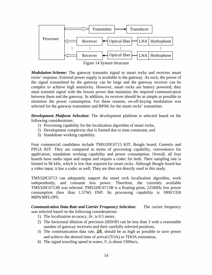
14

Figure 14 System Structure

Modulation Scheme: The gateway transmits signal to smart rocks and receives smart rocks’ response. External power supply is available to the gateway. As such, the power of the signal transmitted by the gateway can be large and the gateway receiver can be complex to achieve high sensitivity. However, smart rocks are battery powered; they must transmit signal with the lowest power that maintains the required communication between them and the gateway. In addition, its receiver should be as simple as possible to minimize the power consumption. For these reasons, on-off-keying modulation was selected for the gateway transmitter and BPSK for the smart rocks’ transmitter. Development Platform Selection: The development platform is selected based on the following considerations:

1) Processing capability for the localization algorithm of smart rocks, 2) Development complexity that is limited due to time constraint, and 3) Standalone working capability.

Four commercial candidates include TMS320C6713 KIT, Beagle board, Gumstix and FPGA KIT. They are compared in terms of processing capability, convenience for application, standalone working capability and power consumption. Overall, all four boards have audio input and output and require a codec for both. Their sampling rate is limited to 96 kHz, which is low that required for smart rocks. Although Beagle board has a video input, it has a codec as well. They are thus not directly used in this study. TMS320C6713 can adequately support the smart rock localization algorithm, work independently, and consume less power. Therefore, the currently available TMS320C6713B was selected. TMS320C6713B is a floating point, 225MHz low power consumption (less than 1.57W) DSP. Its processing capability is 1800/1350 MIPS/MFLOPS. Communication Data Rate and Carrier Frequency Selection: The carrier frequency was selected based on the following considerations:

1) The localization accuracy, , is 0.5 meter, 2) The horizontal dilution of precision (HDOP) can be less than 3 with a reasonable

number of gateway receivers and their carefully selected positions, 3) The communication data rate, , should be as high as possible to save power

and achieve the desired time of arrival (TOA) or TDOA estimation, 4) The signal traveling speed in water, , is about 1500m/s,

RAM

Processor

Transmitter Transducer

Receiver

Receiver

Hydrophone

Hydrophone

LNA

LNA

Optical fiber

Optical fiber

15

5) The modulation and demodulation require at least 10 carrier cycles in each symbol duration, , and

6) The life of the battery on smart rocks should last as long as possible. To achieve the desired localization accuracy, the data rate ( ), signal speed ( ) and

must meet the following inequality: . (1)

To achieve 0.5 m accuracy in smart rock localization, the data rate must be higher than 9 kbps. With 10% redundancy, a data rate of 10 kbps was selected. Considering the modulation and demodulation requirements, the carrier frequency should be higher than 100 kHz. On the other hand, as the signal carrier frequency increases, the signal attenuates more rapidly in water. To maintain low transmitting power and thus a longer battery life, a carrier frequency between 100 kHz and 200 kHz was selected. Transducer Selection: Many transducers are commercially available for military and civil applications. While military products are too expensive to use in civil engineering, most of the available civil transducers have an insufficient beam width for this project. The transducer was selected for smart rocks based on the following considerations:

1) For a symbol rate of over 10kbps, the bandwidth and frequency should be larger than 10 kHz and between 100 kHz and 200 kHz, respectively.

2) The beam width determines how many gateways can receive the signal from a smart rock. Due to the need for a large number of gateways, an Omni-directional or almost Omni-directional transducer is needed.

3) The input power cannot be high and the driving voltage should be low. Based on the commercial availability, a RF45 from Humminbird transducer was selected for its relatively large beam width. In addition, an ANN-P5AT6550560635 from Annon Piezo is acquired to make a new transducer for its Omni directional beam pattern in horizontal direction and for higher frequency. I.2 PROBLEMS ENCOUNTERED During the first quarter of the project, no unexpected technical problem was encountered. We were short of staff, though, specifically for this project. The signed agreement was received on May 31, 2011. A project number was assigned to this specific project after approximately two weeks. As such, we did not have sufficient time to fill all positions. However, work was under way immediately after the signed agreement has been received by the team. Two Ph.D. students who were supported from other sources were asked to participate in this project and keep technical work moving forward in time.

I.3 FUTURE PLANS Three subtasks will be executed during the next quarter. A brief description of various activities in each subtask is described below:

16

Task 1.1 Design, fabricate, and test in laboratory and field conditions DC magnetic sensors with embedded steel in Dodecahedron shape or magnets aligned with the earth gravity field. Summarize and document the test results and the performance of passive smart sensors. Built on the previous work, magnets will be embedded inside concrete blocks in various shapes. Their effectiveness in providing sensitive magnetic field measurements will be systematically characterized. Task 2.2(a) Design, fabricate, and test in laboratory and field conditions magneto-inductive transponders. Summarize and document the test results and the performance of transponders. A controllable magnet system will be built with a permanent magnet and a coil for alternating the polarity of the magnet. Measurements on the transient effect of alternating current on the maximum measurement distance of the magnet and resolution will be taken. The magneto-inductive communication system V2.3 will be expanded with additional capabilities and further tested to achieve consistent and robust measurements. A prototype for laboratory tests will be built and tested before it is sent to the Hydraulic Engineering Laboratory at Turner-Fairbank Highway Research Center, Federal Highway Administration. Task 2.2(b) Research, summarize, and document current underwater acoustic transmission practices and required modifications for bridge scour monitoring. In the following quarter, an acoustic communication system will be built, including one transmitter and one receiver. After it has been tested to satisfaction, a multi-receiver system will be built with capability of smart rock localization. In this case, multiple transducers / hydrophones are distributed to different locations for TDOA estimation. The smart rocks will be located using the TDOA fusion and the assistance of pressure sensor in smart rocks, which provides the elevation information of the smart rocks.

17

II – BUSINESS STATUS II.1 HOURS/EFFORT EXPENDED The planned hours and the actual hours expended on this project are given and compared in Table 1. The actual hours is approximately 25% of the planned hours due to short of staff appointed on this particular project.

Table 1 Hours Expended on This Project

Planned Actual Labor Hours Cumulative Labor Hours Cumulative

Quarter 1 752 752 184 184

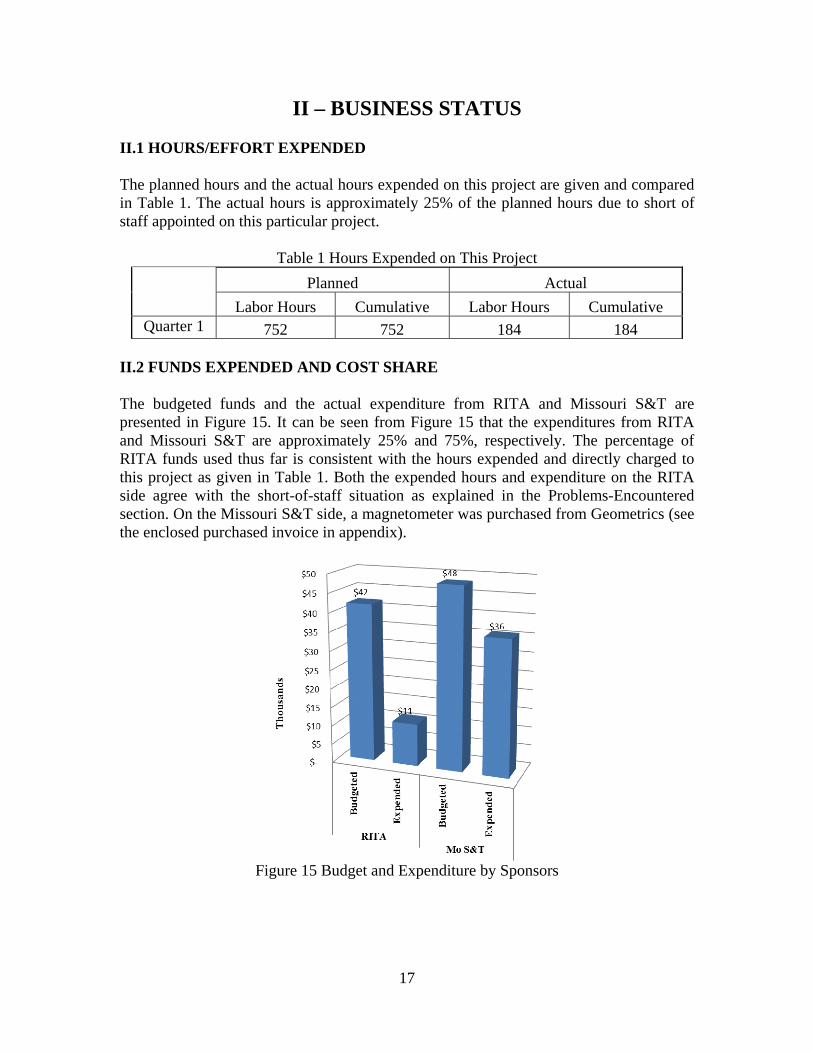
II.2 FUNDS EXPENDED AND COST SHARE The budgeted funds and the actual expenditure from RITA and Missouri S&T are presented in Figure 15. It can be seen from Figure 15 that the expenditures from RITA and Missouri S&T are approximately 25% and 75%, respectively. The percentage of RITA funds used thus far is consistent with the hours expended and directly charged to this project as given in Table 1. Both the expended hours and expenditure on the RITA side agree with the short-of-staff situation as explained in the Problems-Encountered section. On the Missouri S&T side, a magnetometer was purchased from Geometrics (see the enclosed purchased invoice in appendix).

Figure 15 Budget and Expenditure by Sponsors

18

ADVISORY COMMITTEE MEETING The external advisory committee met between 10:30 am and 11:45 am on June 30, 2011, via a teleconference call. Present at the meeting are Dr. Kornel Kerenyi from Turner-Fairbank Highway Research Center at Federal Highway Administration, Mr. Keith Ferrell from Missouri Department of Transportation (MoDOT), Dr. Huimin Mu from the City of San Jose, Mr. Larry Olson from Olson Engineering, Mr. William Porter from WFS Defense, and Dr. Genda Chen. Mr. Ross Johnson from Geometrics was not present due to schedule conflict. Dr. Chen called the meeting in order. Following is a summary of the meeting report.

1) Overview of Project

a) Project Duration Two years

b) Funding Level i) $500,000 from US DOT RITA (cash) ii) $350,000 from MoDOT (in-kind) iii) $166,041 from Missouri S&T (cash + in-kind)

c) Objectives i) Integrate commercial measurement and communication technologies into a

wireless rock positioning system with spatially-distributed smart rocks (both passive and active), and

ii) Evaluate the technologies and improve their performance for scour monitoring at reduced costs, particularly when they are integrated with a rip-rap mitigation strategy.

d) Application Scenarios i) Real-time maximum scour depth monitoring with smart rocks ii) Real-time rip-rap countermeasure effectiveness monitoring with smart rocks

e) Technical Approach The proposed remote sensing technology involves passive and/or active sensors embedded in rocks or reinforced concrete blocks, both referred to as smart rocks, and magneto-inductive or acoustic communications for a real-time engineering evaluation of bridge scour on a Geographic Information System platform. For application scenario #1, smart rocks are deployed around the perimeter of a pier foundation. They will sink into the scour hole as developed. With deposit refilling or not, the smart rocks can give the maximum scour depth, a critical data for engineering design and assessment of bridge scour. For application scenario #2, together with natural rocks, smart rocks are not only distributed around a bridge foundation for scour mitigation but also represent the process of bridge scour as they are washed away.

2) Application parameter ranges for bridge scour monitoring a) Horizontal and vertical movement accurate to within 0.5 meters b) Transmission distance: 5-30 meters

3) Electronics parameter for smart rock design a) Data speed

19

i) Gates transmit data every 15 minutes ii) Small flashy streams need hourly data transfers during flood conditions iii) In flood conditions transmit data as needed, more frequently than in calm river

conditions 4) Potential implementation challenges and solutions with smart rocks

a) Determine the best shape to prevent wash away i) Sphere/octagonal shape to monitor the maximum scour ii) Natural rock shape for scour mitigation

b) Determine how to place smart rocks i) Divers ii) Drop rocks from boat iii) Drops rock from boat and guide with string/chain

5) Others a) Battery life

i) Battery life estimated to last 15 years ii) Life expectancy changes based on the number of data transmissions iii) More frequent measurements are taken during flood conditions and less out of

flood conditions to preserve battery life b) Lab vs. field smart rock

i) No problem to make lab and field scale magnetic passive smart rock ii) More expense and time involved in making both lab and field scale acoustical

smart rock c) Lab test accuracy

i) Function of many variables ii) Need to do many lab tests to determine the minimum movement measured in

the lab

20

APPENDIX: PURCHASE RECEIPT A copy of magnetometer G858 purchase receipt is enclosed in this appendix.