SMAST Technical Report 05-1010

9 September 2016 Yu & Brown ESDIM Temperature Variability SMAST Report 1

SMAST Technical Report 05-1010

Historical Surface Temperature Variability in the Gulf of Maine Region Z. Yu and W. S. Brown

Department of Estuarine and Ocean Sciences School for Marine Science and Technology

University of Massachusetts – Dartmouth New Bedford, MA

A. Introduction

We seek to better understand how well the variability in moored temperatures in Nantucket Shoals region represents that of the larger regional New England coastal ocean. This and other related issues are addressed through a combined analysis of the historical lightship data and shipboard temperature data rescued in the University of Massachusetts’ School for Marine Science and Technology (SMAST) ESDIM project.

B. The Lightship Data

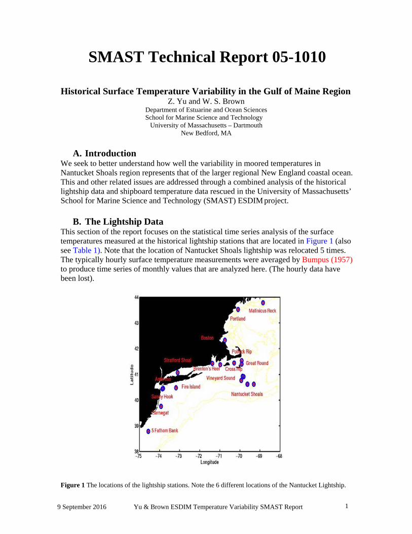
This section of the report focuses on the statistical time series analysis of the surface temperatures measured at the historical lightship stations that are located in Figure 1 (also see Table 1). Note that the location of Nantucket Shoals lightship was relocated 5 times. The typically hourly surface temperature measurements were averaged by Bumpus (1957) to produce time series of monthly values that are analyzed here. (The hourly data have been lost).

Figure 1 The locations of the lightship stations. Note the 6 different locations of the Nantucket Lightship.


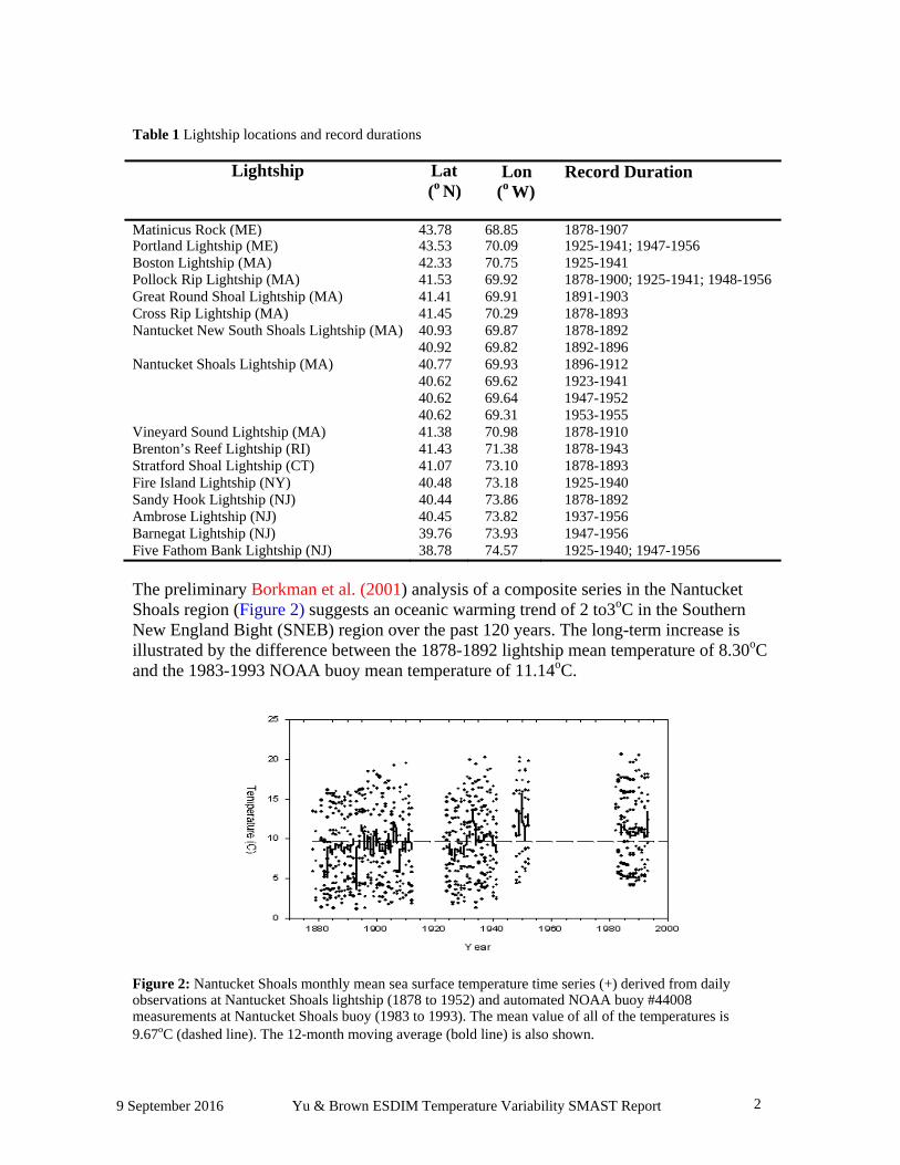
Table 1 Lightship locations and record durations

Lightship Lat (o N)

Lon (o W)

Record Duration

Matinicus Rock (ME) 43.78 68.85 1878-1907Portland Lightship (ME) 43.53 70.09 1925-1941; 1947-1956 Boston Lightship (MA) 42.33 70.75 1925-1941Pollock Rip Lightship (MA) 41.53 69.92 1878-1900; 1925-1941; 1948-1956Great Round Shoal Lightship (MA) 41.41 69.91 1891-1903Cross Rip Lightship (MA) 41.45 70.29 1878-1893Nantucket New South Shoals Lightship (MA) 40.93 69.87 1878-1892

40.92 69.82 1892-1896Nantucket Shoals Lightship (MA) 40.77 69.93 1896-1912

40.62 69.62 1923-1941 40.62 69.64 1947-1952 40.62 69.31 1953-1955

Vineyard Sound Lightship (MA) 41.38 70.98 1878-1910Brenton’s Reef Lightship (RI) 41.43 71.38 1878-1943Stratford Shoal Lightship (CT) 41.07 73.10 1878-1893Fire Island Lightship (NY) 40.48 73.18 1925-1940Sandy Hook Lightship (NJ) 40.44 73.86 1878-1892Ambrose Lightship (NJ) 40.45 73.82 1937-1956Barnegat Lightship (NJ) 39.76 73.93 1947-1956Five Fathom Bank Lightship (NJ) 38.78 74.57 1925-1940; 1947-1956

The preliminary Borkman et al. (2001) analysis of a composite series in the Nantucket Shoals region (Figure 2) suggests an oceanic warming trend of 2 to3oC in the Southern New England Bight (SNEB) region over the past 120 years. The long-term increase is illustrated by the difference between the 1878-1892 lightship mean temperature of 8.30oC and the 1983-1993 NOAA buoy mean temperature of 11.14oC.

Figure 2: Nantucket Shoals monthly mean sea surface temperature time series (+) derived from daily observations at Nantucket Shoals lightship (1878 to 1952) and automated NOAA buoy #44008 measurements at Nantucket Shoals buoy (1983 to 1993). The mean value of all of the temperatures is 9.67oC (dashed line). The 12-month moving average (bold line) is also shown.


As illustrated by the 1878-1907 Brenton’s Reef record (Figure 3) and the 1925-40 Portland record (Figure 4), all of the lightship surface temperature series are dominated by the annual cycle. A problem is that most of these series had numerous temporal gaps. The gaps were filled with values from the station mean annual cycle; one that was locally fit to the real data to minimize discontinuities. (Note: The Matinicus Rock record could not be processed because it lacked data for the winter months). The basic statistics that were computed for each record are presented in Table 2. As expected, the more southern stations were warmer on average and exhibited a larger amplitude annual cycle (as indicated by the standard deviation) than the more northern and eastern stations. The record trends varied between the 0.140oC per month for the relatively short Fire Island record to the 0.003 oC/mo for the moderately long Vineyard Sound record.

Table 2. Lightship time series statistics: number of observed temperatures, series mean, series standard derivation, and series trend. The station series have been clustered according to nominal lengths.

Lightship Start

Year End Year

No. of “Real” Data

Mean

(oC)

STD

(oC)

1925-40 Trend (oC/mo)

Series Trend (oC/mo)

Five Fathom Bank, NJ 1878 1943 402 12.69 7.08 0.007 Brenton’s Reef, RI 1878 1943 756 10.44 6.26 0.006 Nantucket Shoals, MA 1878 1943 522 9.11 4.89 0.014 Pollock Rip, MA 1878 1943 441 8.41 4.56 0.004

Great Round Shoal, MA 1891 1903 135 8.67 5.05 0.100

Vineyard Sound, MA 1878 1907 329 9.71 6.41 0.003 Matinicus Rock, ME 1878 1907 151 9.20 3.15

Fire Island, NY 1925 1940 164 11.63 6.80 0.140 Boston, MA 1925 1940 178 8.98 5.44 0.065 Portland, ME 1925 1940 163 7.22 4.89

Sandy Hook, NJ 1878 1892 152 11.90 6.84 0.053 Stratford Shoal, CT 1878 1892 154 10.95 7.52 0.068 Cross Rip, MA 1878 1892 159 10.02 7.50 0.079

Ambrose, NJ 1947 1956 41 11.23 6.90 0.132 Barnegat, NJ 1947 1956 101 12.94 6.72 0.078

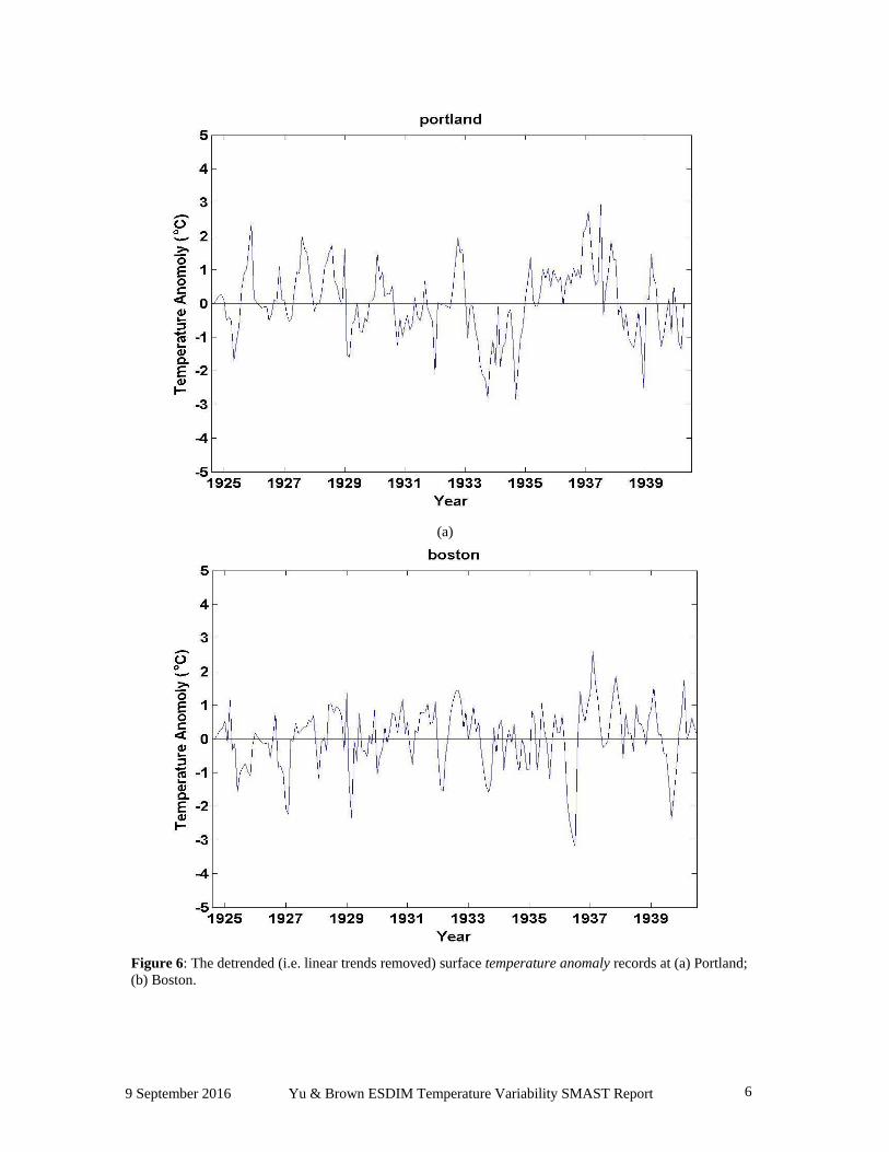
However, there are noticeable year-to-year differences in these records. To explore the interannual variability, the station mean annual cycle was removed from each of the time series to produce the corresponding surface temperature anomaly records. A pair of temperature anomaly records for 1878-1907 (with trend removed) is presented in Figure 5; and for 1925-1940 in Figure 6.


Figure 3 Monthly mean surface temperature at Brenton’s Reef, RI: 1878 to 1907.

Figure 4 Monthly mean surface temperature at Portland, ME: 1925 to 1940.


(a)

(b)

Figure 5: The detrended (i.e. linear trends removed) surface temperature anomaly records at (a) Brenton’s Reef; (b) Vineyard Sound.


(a)

Figure 6: The detrended (i.e. linear trends removed) surface temperature anomaly records at (a) Portland; (b) Boston.


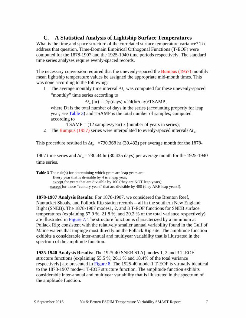
C. A Statistical Analysis of Lightship Surface Temperatures What is the time and space structure of the correlated surface temperature variance? To address that question, Time-Domain Empirical Orthogonal Functions (T-EOF) were computed for the 1878-1907 and the 1925-1940 time periods respectively. The standard time series analyses require evenly-spaced records.

The necessary conversion required that the unevenly-spaced the Bumpus (1957) monthly mean lightship temperature values be assigned the appropriate mid-month times. This was done according to the following:

1. The average monthly time interval tm was computed for these unevenly-spaced “monthly” time series according to

tm (hr) = DT (days) x 24(hr/day)/TSAMP , where DT is the total number of days in the series (accounting properly for leap year; see Table 3) and TSAMP is the total number of samples; computed according to

TSAMP = (12 samples/year) x (number of years in series); 2. The Bumpus (1957) series were interpolated to evenly-spaced intervals tm .

This procedure resulted in tm =730.368 hr (30.432) per average month for the 1878-

1907 time series and tm = 730.44 hr (30.435 days) per average month for the 1925-1940 time series.

Table 3 The rule(s) for determining which years are leap years are:

Every year that is divisible by 4 is a leap year; except for years that are divisible by 100 (they are NOT leap years);

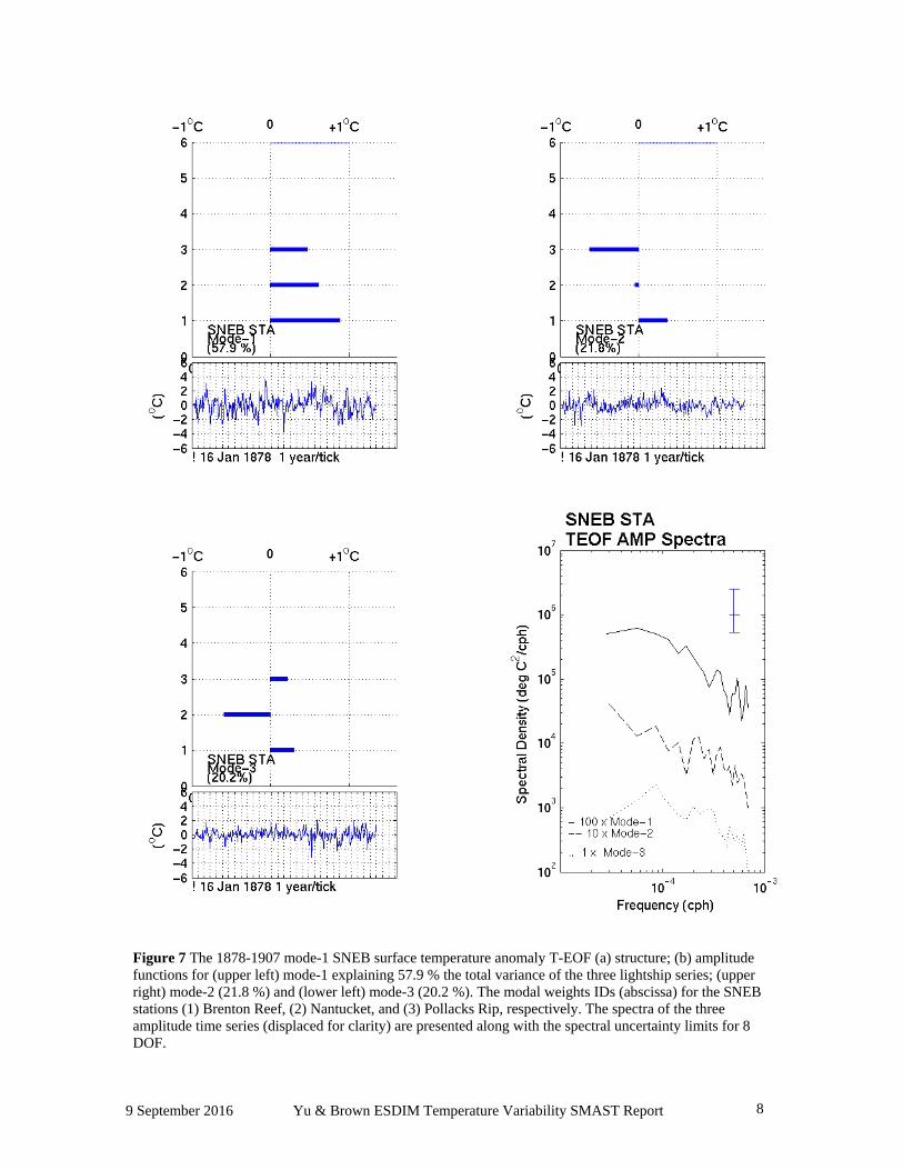
except for those “century years” that are divisible by 400 (they ARE leap years!). 1878-1907 Analysis Results: For 1878-1907, we considered the Brenton Reef, Nantucket Shoals, and Pollock Rip station records – all in the southern New England Bight (SNEB). The 1878-1907 modes1, 2, and 3 T-EOF functions for SNEB surface temperatures (explaining 57.9 %, 21.8 %, and 20.2 % of the total variance respectively) are illustrated in Figure 7. The structure function is characterized by a minimum at Pollack Rip; consistent with the relatively smaller annual variability found in the Gulf of Maine waters that impinge most directly on the Pollack Rip site. The amplitude function exhibits a considerable inter-annual and multiyear variability that is illustrated in the spectrum of the amplitude function.

1925-1940 Analysis Results: The 1925-40 SNEB STA) modes 1, 2 and 3 T-EOF structure functions (explaining 55.5 %, 26.1 % and 18.4% of the total variance respectively) are presented in Figure 8. The 1925-40 mode-1 T-EOF is virtually identical to the 1878-1907 mode-1 T-EOF structure function. The amplitude function exhibits considerable inter-annual and multiyear variability that is illustrated in the spectrum of the amplitude function.


Figure 7 The 1878-1907 mode-1 SNEB surface temperature anomaly T-EOF (a) structure; (b) amplitude functions for (upper left) mode-1 explaining 57.9 % the total variance of the three lightship series; (upper right) mode-2 (21.8 %) and (lower left) mode-3 (20.2 %). The modal weights IDs (abscissa) for the SNEB stations (1) Brenton Reef, (2) Nantucket, and (3) Pollacks Rip, respectively. The spectra of the three amplitude time series (displaced for clarity) are presented along with the spectral uncertainty limits for 8 DOF.


Figure 8 The 1925-1940 SNEB STA TEOF structure and amplitude functions for (upper left) mode-1 explaining 55.5 % the total variance of the three lightship series; (upper right) mode-2 (26.1 %) and (lower left) mode-3 (18.4 %). The modal weights IDs (abscissa) for the SNEB stations (1) Brenton Reef, (2) Nantucket, and (3) Pollacks Rip, respectively. The spectra of the three amplitude time series (displaced for clarity) are presented along with the spectral uncertainty limits for 8 DOF.


The 1925 SNEB/GOM STA modes 1, 2 and 3 T-EOF structure functions (explaining 42.7 %, 21.6 % and 14.6 % of the total variance respectively), which are presented in Figure 9 are consistent with the SNEB STA T-EOF results.

Figure 9 The 1925-1940 SNEB/GOM STA TEOF structure and amplitude functions for (upper left) mode- 1 explaining 42.7% the total variance of the five lightship series; (upper right) mode-2 (21.6 %) and (lower left) mode-3 (14.6%). The modal weights IDs (abscissa) pertain to (1) Brenton Reef, (2) Nantucket, (3) Pollack Rip, (4) Boston, and (5) Portland, respectively. The spectra of the three amplitude time series (displaced for clarity) are presented along with the spectral uncertainty limits for 8 DOF.

The 1878-1907 SNEB STA mode 1 TEOF amplitude function was cross-correlated (see Appendix A) with the Winter North Atlantic Oscillation Index (WNAOI). The cross- correlation showed a very weak, but statistically significant cross-correlation in which the SNEB STA TEOF lagged NAOWI by 15 to 20 months.


The 1925-1940 SNEB STA mode 1, 2 and 3 TEOF amplitude functions are compared with the WNAOI in Figure 10. Interestingly the best visual match is between the mode-2 amplitude function and the WNAOI. In fact, the cross-correlation of mode-2 T-EOF SNEB/GOM amplitude function versus the NAO Winter Index (Appendix B) shows a very weak, but statistically significant cross-correlation, in which the SNEB STA TEOF lags the NAOWI by 28 to 30 months.

Figure 10 The mode-1, mode-2, and mode-3 TEOF amplitude functions (dotted) for the 1925-1940 SNEB STA trio (Brenton Reef, Nantucket, and Pollack Rip) are compared with the NAO Winter Index (solid red).

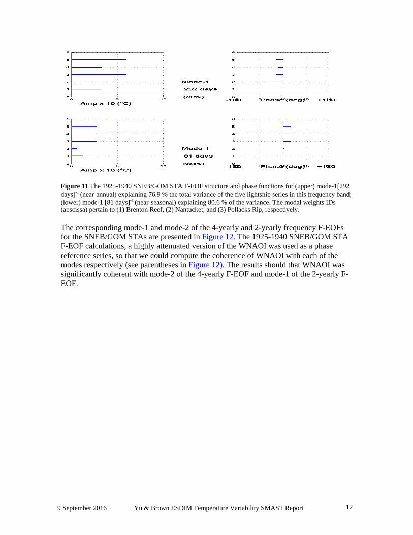
Frequency Domain Empirical Functions (F-EOF) were computed to obtain a more incisive quantitative description of the STA variability. The 1925-1940 SNEB/GOM STA mode-1 F-EOFs for near-annual frequency ([292 days]-1) and near-seasonal ([81 days]-1) frequency bands respectively, are presented in Figure 11.


Figure 11 The 1925-1940 SNEB/GOM STA F-EOF structure and phase functions for (upper) mode-1[292 days]-1 (near-annual) explaining 76.9 % the total variance of the five lightship series in this frequency band; (lower) mode-1 [81 days]-1 (near-seasonal) explaining 80.6 % of the variance. The modal weights IDs (abscissa) pertain to (1) Brenton Reef, (2) Nantucket, and (3) Pollacks Rip, respectively.

The corresponding mode-1 and mode-2 of the 4-yearly and 2-yearly frequency F-EOFs for the SNEB/GOM STAs are presented in Figure 12. The 1925-1940 SNEB/GOM STA F-EOF calculations, a highly attenuated version of the WNAOI was used as a phase reference series, so that we could compute the coherence of WNAOI with each of the modes respectively (see parentheses in Figure 12). The results should that WNAOI was significantly coherent with mode-2 of the 4-yearly F-EOF and mode-1 of the 2-yearly F- EOF.


Figure 12 The 1925-1940 SNEB STA F-EOF structure and phase functions for (upper) modes-1 and -2 of the 4-yearly frequency, explaining 63.3 % and 22.4 % of the total variance respectively; (lower) modes-1 and -2 of the 2-yearly frequency explaining 62.4 % and 26.1 % of the variance respectively. The modal weights IDs (abscissa) pertain to (1) Brenton Reef, (2) Nantucket, (3) Pollack’s Rip, (4) Boston, and (5) Portland respectively.


D. Shipboard Surface Temperature Maps The SMAST ESDIM temperature database, covering the time interval 1837 to 1945, consists of 18744 data entries, with 12354 surface temperature measurements. While these temperature data are distributed throughout a region bounded by longitudes between 100oW to 0o and latitudes between the equator and 80oN, most of the data are found along the North American east coast (Figure 13). Moreover half of the surface temperatures (6902) are located in the Gulf of Maine region, with greatest concentrations in Buzzards Bay and Massachusetts Bay (see Figure 14).

Figure13 The distribution map of the 12354 SMAST ESDIM surface temperature data.

Figure 14 The distribution map of the 6902 SMAST ESDIM surface temperature data in the Gulf of Maine region.


The data in the Gulf of Maine region bounded by longitudes 71oW to 66oW and latitudes 40oN and 45oN have been extracted from the database 5-year time bins for the summers (defined as July through September) of 1870 through 1909 (see http://www.smast.umassd.edu/Fisheries/OCEANOL/reports.php). These 5-year summer data were used to generate the suite of surface temperature maps that are presented in Figures 15-21 (data indicated by *).

Figure 15 Summer 1870-1875 surface temperature map (data = *).




. Figure 18 Summer 1885-1890 surface temperature map (data = *).



. Figure 20 Summer 1900-1905 surface temperature map (data = *).



The surface temperature data is particularly dense in Buzzards Bay (71.5 -70.3oW; 41 - 42oN) between years 1900 to 1910 (Figure 22) with the greatest concentrations in August (Figure 23). The August 1904 temperature map is shown in Figure 24.

Figure 22 The distribution of surface temperature data in the Buzzards Bay region by year as indicated by the color bar to the right.


Figure 23 The 1901-10 distribution of surface temperature data in the Buzzards Bay region by month as indicated by the color bar to the right.

Figure 24 Summer 1904 surface temperature in Buzzards Bay.


E. AFAP Hydrographic Profiles Hydrographic profiles between 1925 and 1940 were extracted for Wilkinson Basin and Georges Basin area from Bedford Institute of Oceanography hydrographic database (http://www.mar.dfo-mpo.gc.ca/science/ocean/database/data_query.html). The Wilkinson Basin area was defined by a box; -70.5o to -68.5 o E longitude and 41.5 o to 43.0 o N latitude. The Georges Basin area was defined by a box; -68.0 o to -66.5 o E longitude and 42.0 o to 43.0 o N latitude. For the analysis below, the profiles are all deeper than 150 meter for Wilkinson Basin and 100 meters for Georges Basin area.

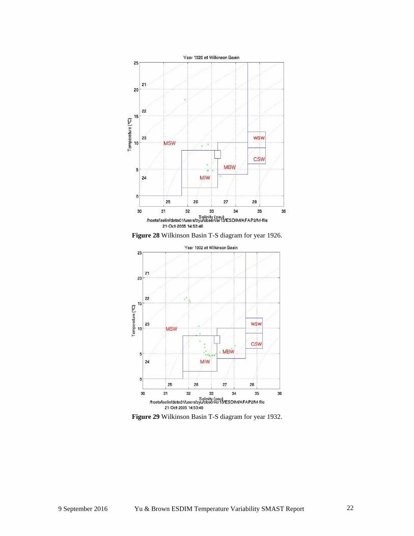
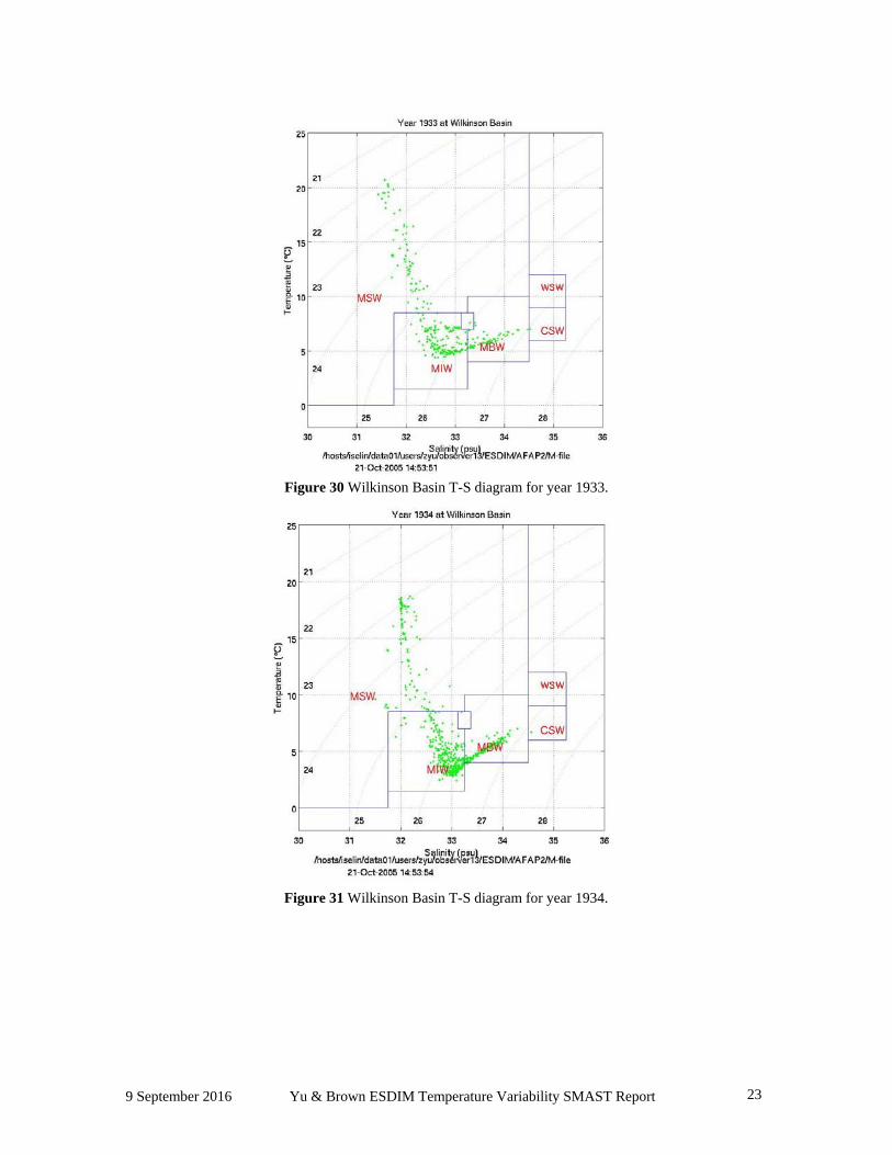
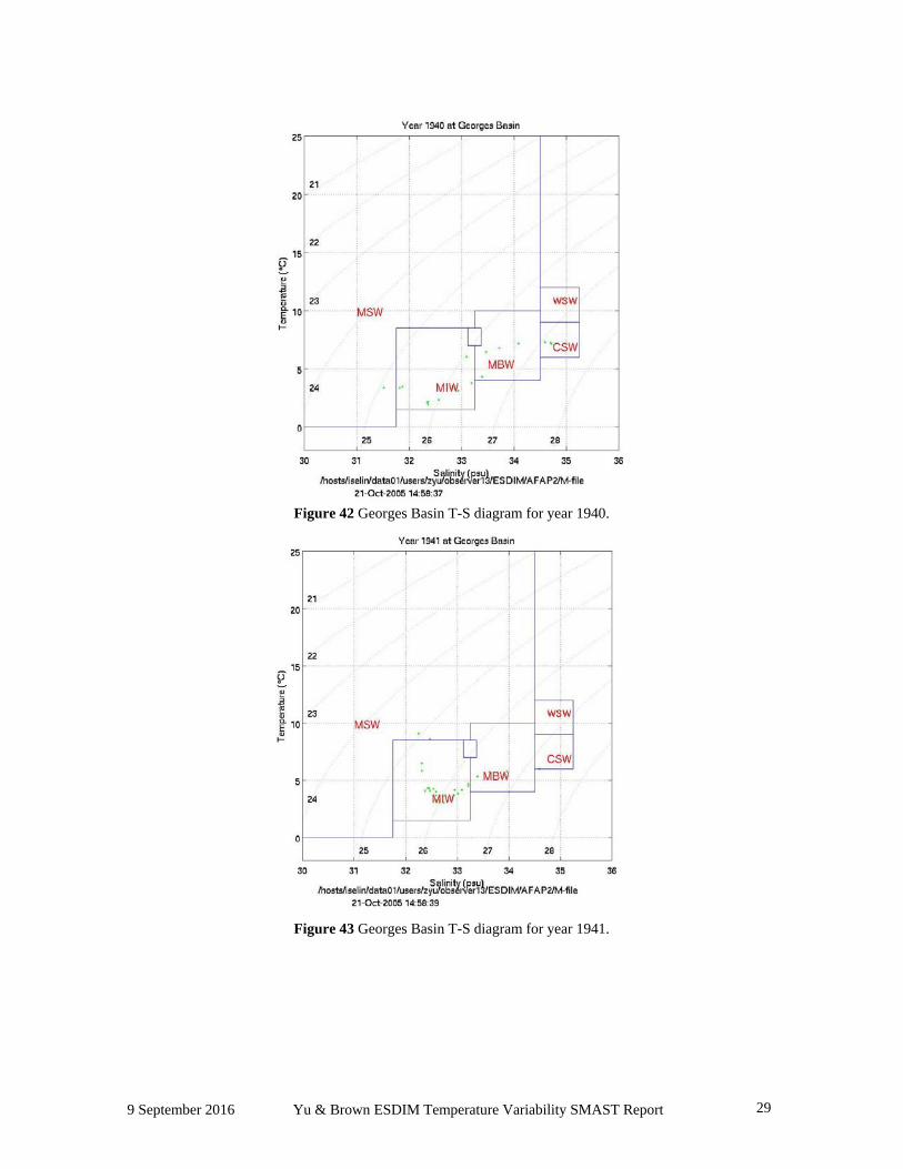
There were a total of 122 profiles in Wilkinson Basin (See Figure 25) and 70 profiles at Georges Basin (see Figure 26) distributed unevenly from 1925 to 1945. Whenever profiles are available, the yearly T-S diagram was generated. All these T-S diagrams clearly show the Maine Intermediate Water (MIW) and the mixing with Cold Slope Water (CSW) to form Maine Bottom Water (MBW) (See Figure 27 to 43). There was no evidence of Warm Slope water in these data.

Figure 25 Yearly distribution of AFAP profiles located at Wilkinson Basin area from 1920 to 1945.


Figure 26 Yearly distribution of AFAP profiles located at Georges Basin area from 1920 to 1945.

Figure 27 Wilkinson Basin T-S diagram for year 1925.














Figure 36 Georges Basin T-S diagram for year 1926.












F. Appendices A. The 1878-1907 SNEB STA Trio - NAOWI Cross-Correlations The tabulated cross-correlation of TEOF mode-1 amplitude function versus the NAO Winter Index (integral time scale =3597.772hr or 4.9 months) shows a very weak, but statistically significant cross-correlations (highlighted) between NAOWI (v) and a SNEB STA TEOF (u) that lags by 15 to 20 months .

Normalized long lag (Sciremammano, 1979) cross-correlations (i.e. *cuv) > 2.0 are statistically significant at the 95% confidence level. Definitions - cuv+ = cross-correlation function at + time lags

cuv- = cross-correlation function at - time lags *cuv+= normalized cross-correlation function at + time lags *cuv- = normalized cross-correlation function at - time lags std err = long-lag standard error

lag time cuv+ cuv- *cuv+ *cuv- std err (hr)

0.0000 -5.6580E-02 -5.6580E-02 -4.8373E-01 -4.8373E-01 1.1696E-01 730.5000 -2.2031E-02 -8.9998E-02 -1.8810E-01 -7.6837E-01 1.1713E-01

1461.0000 1.1295E-02 -1.1893E-01 9.6301E-02 -1.0140E+00 1.1729E-012191.5000 4.1321E-02 -1.4134E-01 3.5180E-01 -1.2034E+00 1.1746E-012922.0000 6.5974E-02 -1.5282E-01 5.6091E-01 -1.2992E+00 1.1762E-013652.5000 8.3871E-02 -1.5197E-01 7.1206E-01 -1.2902E+00 1.1779E-014383.0000 9.4401E-02 -1.3763E-01 8.0034E-01 -1.1668E+00 1.1795E-015113.5000 9.6988E-02 -1.1531E-01 8.2111E-01 -9.7623E-01 1.1812E-015844.0000 9.0408E-02 -8.1622E-02 7.6431E-01 -6.9003E-01 1.1829E-016574.5000 7.8176E-02 -3.6499E-02 6.5996E-01 -3.0812E-01 1.1845E-017305.0000 6.1712E-02 1.7335E-02 5.2024E-01 1.4613E-01 1.1862E-018035.5000 4.0491E-02 7.2806E-02 3.4085E-01 6.1288E-01 1.1879E-018766.0000 1.9122E-02 1.2942E-01 1.6073E-01 1.0879E+00 1.1896E-019496.5000 -3.0262E-03 1.8001E-01 -2.5402E-02 1.5109E+00 1.1914E-01

10227.0000 -2.1574E-02 2.2462E-01 -1.8083E-01 1.8827E+00 1.1931E-0110957.5000 -3.6061E-02 2.6067E-01 -3.0181E-01 2.1817E+00 1.1948E-0111688.0000 -4.4945E-02 2.8320E-01 -3.7563E-01 2.3668E+00 1.1965E-0112418.5000 -4.5756E-02 2.9728E-01 -3.8185E-01 2.4809E+00 1.1983E-0113149.0000 -4.0166E-02 2.9554E-01 -3.3470E-01 2.4628E+00 1.2000E-0113879.5000 -2.8785E-02 2.8405E-01 -2.3952E-01 2.3636E+00 1.2018E-0114610.0000 -1.2056E-02 2.6147E-01 -1.0017E-01 2.1725E+00 1.2036E-0115340.5000 8.0449E-03 2.3287E-01 6.6744E-02 1.9320E+00 1.2053E-0116071.0000 3.0945E-02 1.9802E-01 2.5635E-01 1.6405E+00 1.2071E-0116801.5000 5.1943E-02 1.6271E-01 4.2967E-01 1.3459E+00 1.2089E-0117532.0000 7.2297E-02 1.2840E-01 5.9715E-01 1.0605E+00 1.2107E-0118262.5000 9.0460E-02 9.6333E-02 7.4606E-01 7.9449E-01 1.2125E-0118993.0000 1.0300E-01 6.6833E-02 8.4825E-01 5.5037E-01 1.2143E-0119723.5000 1.0894E-01 4.6250E-02 8.9580E-01 3.8030E-01 1.2161E-0120454.0000 1.0711E-01 3.3287E-02 8.7940E-01 2.7330E-01 1.2180E-0121184.5000 1.0018E-01 3.3091E-02 8.2125E-01 2.7128E-01 1.2198E-0121915.0000 8.7024E-02 3.8622E-02 7.1234E-01 3.1615E-01 1.2217E-01


B. The 1925-1940 SNEB STA Quintet - NAOWI Cross-Correlations The tabulated cross-correlation of TEOF mode-2 amplitude function versus the NAO Winter Index (integral time scale = 4171 hours or 5.7 months) shows a very weak, but statistically significant cross-correlations (highlighted) between NAOWI (v) and a SNEB STA TEOF (u) that lag by 28 to 30 months .

Normalized long lag (Sciremammano, 1979) cross-correlations (i.e. *cuv) > 2.0 are statistically significant at the 95% confidence level. Definitions - cuv+ = cross-correlation function at + time lags

cuv- = cross-correlation function at - time lags *cuv+= normalized cross-correlation function at + time lags *cuv- = normalized cross-correlation function at - time lags std err = long-lag standard error

lag time cuv+ cuv- *cuv+ *cuv- std err (hr) 0.0000 -1.9211E-01 -1.9211E-01 -1.1140E+00 -1.1140E+00 1.7245E-01

730.4293 -1.6828E-01 -2.0494E-01 -9.7326E-01 -1.1853E+00 1.7290E-011460.8586 -1.4406E-01 -2.0981E-01 -8.3101E-01 -1.2103E+00 1.7336E-012191.2880 -1.2043E-01 -2.0655E-01 -6.9286E-01 -1.1883E+00 1.7382E-012921.7173 -9.8364E-02 -1.9572E-01 -5.6441E-01 -1.1230E+00 1.7428E-013652.1466 -7.8547E-02 -2.0051E-01 -4.4950E-01 -1.1475E+00 1.7474E-014382.5759 -6.1353E-02 -1.7907E-01 -3.5016E-01 -1.0220E+00 1.7521E-015113.0052 -4.7196E-02 -1.4843E-01 -2.6864E-01 -8.4485E-01 1.7569E-015843.4346 -3.3319E-02 -1.1513E-01 -1.8914E-01 -6.5354E-01 1.7616E-016573.8639 -2.1804E-02 -8.1272E-02 -1.2344E-01 -4.6009E-01 1.7664E-017304.2932 -1.3098E-02 -4.1708E-02 -7.3949E-02 -2.3547E-01 1.7713E-018034.7225 -6.8544E-03 -8.5016E-03 -3.8591E-02 -4.7865E-02 1.7762E-018765.1518 -2.8925E-04 3.1091E-02 -1.6240E-03 1.7456E-01 1.7811E-019495.5812 9.3748E-03 6.8916E-02 5.2489E-02 3.8586E-01 1.7861E-01

10226.0105 2.3885E-02 1.1640E-01 1.3336E-01 6.4990E-01 1.7911E-0110956.4398 4.2452E-02 1.7209E-01 2.3635E-01 9.5811E-01 1.7961E-0111686.8691 6.5405E-02 2.2923E-01 3.6312E-01 1.2727E+00 1.8012E-0112417.2984 9.2871E-02 2.6184E-01 5.1414E-01 1.4495E+00 1.8064E-0113147.7277 1.2157E-01 2.9360E-01 6.7111E-01 1.6207E+00 1.8115E-0113878.1571 1.5045E-01 3.3267E-01 8.2813E-01 1.8311E+00 1.8168E-0114608.5864 1.7964E-01 3.3803E-01 9.8594E-01 1.8552E+00 1.8220E-0115339.0157 2.0885E-01 3.4101E-01 1.1429E+00 1.8661E+00 1.8274E-0116069.4450 2.3818E-01 3.4208E-01 1.2996E+00 1.8665E+00 1.8327E-0116799.8743 2.6610E-01 3.2752E-01 1.4477E+00 1.7818E+00 1.8381E-0117530.3037 2.9329E-01 3.0322E-01 1.5909E+00 1.6447E+00 1.8436E-0118260.7330 3.2017E-01 2.6796E-01 1.7315E+00 1.4491E+00 1.8491E-0118991.1623 3.4636E-01 2.2415E-01 1.8675E+00 1.2086E+00 1.8547E-0119721.5916 3.6776E-01 2.0169E-01 1.9769E+00 1.0842E+00 1.8603E-0120452.0209 3.8367E-01 1.6422E-01 2.0561E+00 8.8006E-01 1.8659E-0121182.4503 3.9203E-01 1.2798E-01 2.0945E+00 6.8380E-01 1.8717E-0121912.8796 3.9341E-01 7.7298E-02 2.0955E+00 4.1172E-01 1.8774E-01


G. Acknowledgements We are indebted to the earlier efforts of great many people, who over the past seven years were involved in assembling the historical water property and biological data into earlier versions of the SMAST ESDIM database, including in particular R. Hopcroft, D. Borkman, D. Rittmuller, and F. Smith. That work and the more recent efforts have been funded through a series of subcontracts to SMAST (B. J. Rothschild) under PI K. Sherman’s (NMFS, Narragansett, RI) NOAA/ NMFS 03-14.

H. References

Borkman, D., R.R. Hopcroft, J.T. Turner, and B.J. Rothschild, 2001. Rescue of ~160-

year data sets for NE Shelf oceanographic regime assessment. ESDIM (Environmental Services Data and Information Management) Status Report, 37 pp.

Bumpus, D. F. 1957. Surface water temperatures along the Atlantic and Gulf Coasts of the

United States. US Dept. Interior Fish and Wildlife Service Special Scientific Reports – Fisheries #214. 153 pp.

Sciremammano, F. 1979. A suggestion for the presentation of correlations and their

significance levels, J. Phys. Oceanogr., 9, 1273-1276.

Documents

SMAST Technical Report 05-1010