SML Estimation Based on First Order Conditions†

By

Michael P. Keane Department of Economics

Yale University New Haven, CT 06520-8264

michael.keane@yale.edu

November, 2003

† The statistical analysis of the confidential firm-level data on U.S. multinational corporations reported in this study was conducted at the International Investment Division, Bureau of Economic Analysis, U.S. Department of Commerce, under arrangements that maintained legal confidentiality requirements. Seminar participants at Princeton and the University of Minnesota provided useful comments. Conversations with Penny Goldberg, Lee Ohanian, Tom Holmes, Sam Kortum and Chris Sims were also very helpful. All remaining errors are of course my own.

Abstract

This paper describes a strategy for structural estimation of economic models that I will

refer to as SML based on FOCs. In this approach, one uses simulated maximum likelihood

(SML) to estimate the structural parameters that appear in the Euler or first order conditions

(FOCs) solved by an optimizing economic agent.

I will argue that the SML based on FOCs approach has certain advantages over the

generalized method of moments (GMM) approach to structural estimation based on FOCs. Most

importantly, the SML based on FOCs approach can easily handle economic models that involve

multiple structural sources of error. In contrast, GMM requires that all the structural sources of

error enter the FOCs additively, so that a single composite additive error term may be obtained.

In models with multiple sources of error, very strong assumptions on functional form or on

information structure are often necessary in order to put FOCs in this form. Thus, the SML based

on FOCs approach gives the econometrician much more flexibility in terms of how he/she can

specify utility functions and/or production functions, particularly in terms of how these functions

may be heterogeneous across agents.

Implementation of the SML based on FOCs approach requires the development of a

number of new simulation algorithms that I develop here. These include two new recursive

importance sampling algorithms that are the discrete/continuous and purely continuous data

analogues the GHK algorithm for discrete data. These algorithms should have wide applicability

to a range of econometric problems beyond the specific issues discussed here.

I illustrate the SML based on FOCs approach by using it to estimate a structural model of

the behavior of U.S. MNCs with affiliates in Canada. The model is estimated on confidential

BEA firm level data on the activities of U.S. MNCs over the period 1983-96. The method

appears to work well in practice. That is, the computation time was manageable, and the

algorithm converged steadily to stable estimates that were not very sensitive to starting values or

simulation size. The estimated model fits the data reasonably well, and there appeared to be little

evidence against the distributional assumptions that were required to implement the SML

approach.

1

I. Introduction This paper describes a strategy for structural estimation of economic models that I will

refer to as SML based on FOCs. In this approach, one uses simulated maximum likelihood (SML) to estimate the structural parameters that appear in the Euler or first order conditions (FOCs) solved by an optimizing economic agent. I will argue that the SML based on FOCs approach has certain advantages over the generalized method of moments (GMM) approach to structural estimation based on FOCs.

The GMM approach of Hansen (1982) and Hansen and Singleton (1982)) has been popular (at least in part) because it is widely perceived as having one key advantage over a full information maximum likelihood (FIML) approach. Namely, in the GMM approach the econometrician does not need to completely specify the economic model in order to obtain estimates. There are two common ways in which a complete specification is avoided. First, if the FOCs involve expectation terms, it is common to substitute realized quantities for expected quantities, invoke a rational expectations assumption, and then assert that the forecast errors are orthogonal to the elements of agents’ information sets at the time forecasts were made (see McCallum (1976)). Second, if the model structure is such that expectation errors and other structural sources of error (e.g., taste shocks, productivity shocks, etc.) enter the FOCs in a linearly additive fashion, then it is not necessary for the econometrician to specify their joint distribution parametrically. Rather, it is only necessary to assume that the composite error term (obtained by summing the structural errors) is mean independent of a specified set of instruments. One can then obtain moment conditions on which a GMM estimator is based. I would argue however, that the assumptions necessary to put economic models into a form amenable to GMM estimation are often quite strong. Specifically, plausible economic models often involve multiple structural sources of error. In such cases, very strong assumptions on functional form or on information structure may be necessary in order to obtain FOCs where all the structural sources of error enter additively, so that a single composite additive error term may be obtained. A prime example of this problem is provided in the recent paper by Krusell, Ohanian, Rios-Rull and Violante (2000). They estimate a production function with quality of skilled and unskilled labor as two latent stochastic inputs. The FOCs of their model also contain an unmeasured expectation of next period’s price of capital. Thus, three stochastic terms enter nonlinearly, so the FOCs cannot be written in terms of a single additive error. Thus, Krusell et el. cannot use GMM. To deal with this problem, they developed a simulated pseudo-ML procedure for estimation based on FOCs. In this procedure, they assume that the forecast errors and the two

2

shocks to the quality of skilled and unskilled labor are normally distributed. The present paper is very closely related to Krusell, Ohanian, Rios-Rull and Violante (2000). However, I further extend and develop their approach in a number of ways. First, I show how to implement maximum likelihood as opposed to a pseudo-maximum likelihood procedure. Second, I show how to relax normality (via the Box-Cox transformation). Third, I show how to simulate the posterior distributions of the stochastic terms (conditional on the estimated model and the data) of the model. Given draws from the posterior distributions, one can test the distributional assumptions that underlie the SML approach. Testing distributional assumptions is particularly important here, given that the main reason for preferring GMM over a likelihood based procedure is concern over violation of distributional assumptions. The SML based on FOCs approach developed here represents a compromise between a FIML approach and a GMM approach. As in GMM, one does not need a completely specified model. That is, one can avoid having to specify stochastic processes for all of the exogenous forcing variables that impact the environment of the agents. For instance, one can substitute realizations for expectations terms, and invoke a rational expectations assumption to deal with the resulting error terms. But, as in FIML, one must specify the joint distribution of all the structural sources of error (e.g., taste and technology shocks as well as forecast errors). In my view, the SML based on FOCs approach has a number of potential advantages over GMM. A key advantage is that the SML approach can easily handle multiple structural sources of error entering the FOCs in a highly nonlinear way. This gives the econometrician the ability to be much more flexible in terms of how he/she specifies utility functions and/or production functions, particularly in terms of how these functions may be heterogeneous across agents. In my view it is ironic that researchers often claim to be using GMM in order to avoid making distributional assumptions on stochastic terms, yet at the same time they are often willing to make extremely restrictive modeling assumptions in other dimensions (i.e., the functional forms of utility and production functions, how heterogeneity enters the model, etc.) in order to put a model in a form amenable to a GMM approach.1

Another key advantage is that the researcher does obtain estimates of the distributions of the agent specific stochastic terms, and there are many contexts where these distributions are themselves of interest. This advantage is made clear by the particular illustrative application of the SML based on FOCs method that I present in this paper.

It is difficult to describe the SML based on FOCs approach to structural estimation in a 1 Ackerberg and Caves (2003) provide an interesting discussion of the restrictive implications of models of firm behavior in which the number of structural sources of error is less than the number of factor inputs.

3

fully general context, because many of the details of how to implement the procedure will necessarily be specific to the particular economic model being studied. Thus, in this paper I illustrate the SML based on FOC approach by showing how to use it to estimate a particular model of the production and trade decisions of U.S. MNCs with affiliates in Canada. This model has been developed by Feinberg and Keane (2003a), and it gives a good illustration of how the approach works.

I should also stress that the SML based on FOCs approach is not a new estimation method. It is simply an application of SML, whose asymptotic properties have been developed, for example, in Lee (1992, 1995). Thus, I present no proofs of consistency and asymptotic normality for this method, since no new proofs are required. Rather, SML based on FOCs is a new strategy for structural estimation of economic models. That is, to my knowledge, SML has not previously been applied to estimate structural parameters using FOCs. It turns out that implementation of SML in this context is not at all straightforward. It requires the solution of a number of computational problems that do not arise in contexts where SML has previously been applied (such as estimation of discrete choice models), and therefore requires the development of a number of new simulation algorithms. Thus, to be clear, what is new in this paper is: (1) the suggestion of the SML based on FOCs strategy, and (2) the development of several new simulation algorithms necessary to implement that strategy. These new simulation algorithms are of independent interest, as they have broader applicability as well.

The particular empirical application to MNC behavior that I present illustrates well the potential advantages of SML based on FOCs over either FIML or GMM. The structural model of firm behavior that I consider is dynamic, because it allows for labor force adjustment costs. Hence, estimation using FIML would require one to specify how firms form expectations of future labor force size. This in turn would depend on the stochastic processes for several exogenous forcing variables: demand shocks, technology shocks, factor input prices, tariffs, exchange rates, etc.. It is easy to see how a researcher might feel reasonably comfortable specifying functional forms for the MNC production function, as well as for the product demand functions that the MNC faces, while being very reluctant to specify stochastic processes for all these forcing processes. The ability to avoid such assumptions is an advantage over FIML.

On the other hand, a researcher might well wish to specify a production function with several inputs, where the several parameters mapping these inputs into output are allowed to be heterogeneous across firms in a flexible way. As illustrated by the Krusell, Ohanian, Rios-Rull and Violante (2000) paper, allowing multiple production function parameters to be stochastic precludes putting the model in a form amenable to GMM estimation. However, this poses no

4

problem for the SML based on FOCs approach. This is its main advantage over GMM. A key feature of the model is that the stochastic terms are all continuous, yet they must

fall in certain sub-regions of a high dimensional space in order for firm behavior to be rationalizable by the model. In other words, the FOCs cannot be satisfied if certain subsets of the vector of stochastic terms fall in certain regions of the error space. As a result, a high dimensional integral must be evaluated to construct the joint density of a firm’s stochastic terms. In order to evaluate such integrals, I present a new recursive probability simulator that is the discrete/continuous analogue to the GHK method for simulation of discrete choice probabilities (see Keane (1994)).

This new simulator should have wide applicability in discrete/continuous simulation problems, just as GHK has been useful in a wide range of discrete choice problems. For instance, it could be useful in any situation where, in certain regions of the space of stochastic terms, a corner solution is induced where a firm would shut down, discontinue certain products or activities, etc., and where one wants to simulate the density of observed marginal decisions conditional on the firm being active, engaging in certain activities, etc.

Another aspect of the model, which is generic to situations where multiple stochastic terms enter the FOCs nonlinearly, is that the Jacobian of the transformation from the stochastic terms to the data is intractably complex. Thus, since the likelihood is the density of the stochastic terms times this Jacobian, one cannot even writer down the likelihood analytically. Nevertheless, I show how to construct a simulated numerical approximation to the Jacobian. This is what makes it possible to implement a likelihood based estimator (as opposed to the pseudo-ML estimator in Krusell et al.).

Finally, the illustrative model that I estimate here has 14 stochastic terms, yet it is estimated based on 12 FOCs. Models that allow for flexible patterns of heterogeneity in the agent specific parameters will typically have more stochastic terms than there are FOCs. For instance, the MNC production function I estimate here has a stochastic term associated with each input, and the number of FOCs is equal to the number of inputs. But then there are additional stochastic terms associated with expectation errors.

Thus, in order to generate the posterior distribution of the stochastic terms in the model conditional on the data, we need to simulate a J×1 vector of continuous random variables subject to the constraint that it lies in a K×1 dimensional space (where K<J). In order to this I develop a new recursive simulator for purely continuous distributions that is the continuous data analogue of the GHK method (Obviously this is a rather general problem that may arise in many contexts).

When I test the distributional assumptions of the model of MNC behavior by simulating

5

the posterior distributions of the stochastic terms, I find that the distributions of the forecast errors appear strikingly close to normal. Statistical tests do not reject normality even at very low levels of significance. One argument for favoring GMM for the estimation of dynamic structural models based on FOCs is that we have no basis in theory for imposing distributional assumptions on forecast errors. Thus, the finding here that normality is not rejected is quite interesting.

The outline of the remainder of the paper is as follows. Sections II and III present the model of MNC behavior that I will use to illustrate the SML based on FOCs approach. Section IV shows how this model can be estimated using the SML based on FOCs approach. Section V presents the recursive simulation algorithm for simulating from the posterior distribution of the model parameters. Section VI describes the estimation results, including the tests of distributional assumptions. Section VII concludes. II. The Illustrative Model II.1. Overview

This section presents a model of the marginal production and trade decisions of a U.S. MNC with an affiliate in Canada, conditioning on the MNC’s decision to place an affiliate in Canada. Each period, the MNC chooses the levels of factor inputs to utilize in both the U.S. and Canada. In addition, it chooses the levels of four types of trade flows: arms-length imports and exports, and intra-firm trade in intermediates from parent to affiliate and vice versa. Feinberg and Keane (2003a) develop and estimate a model of MNC behavior, and I will use that model to illustrate the SML based on FOCs approach.

The key assumptions of the Feinberg and Keane (2003a) model are as follows: 1) The parent and affiliate each produce a different good. 2) The good produced by the affiliate may serve a dual purpose: it can be sold as a final

good to third parties (in Canada or the U.S.), or it may be used as an intermediate input by the parent. We make a symmetric assumption for the good produced by the parent.

3) Both the parent and affiliate have market power in final goods markets. They each produce a variety of a differentiated product. These products are non-rival (i.e., not substitutes).

4) The parent and affiliate both produce output using a CRTS Cobb-Douglas production function that takes labor, capital and materials as inputs. In addition, intermediates produced by the affiliate may be a required input in the parent’s production process, and intermediates produced by the parent may be a required input in the affiliate’s production process.

5) The affiliate and the parent both face iso-elastic demand functions in both the U.S. and Canadian final goods markets.

6

6) The parent and affiliate both face labor force adjustment costs. 7) The MNC maximizes the expected present value of profits in U.S. dollars, converting

Canadian earnings to U.S. dollars using the nominal exchange rate. 8) The expected rate of profit is equalized across firms. 9) Parameters of technology and of demand are allowed to be heterogeneous both across

firms and within firms over time. Feinberg and Keane (2003a) estimate this model using the Benchmark and Annual

Surveys of U.S. Direct Investment Abroad administered by the Bureau of Economic Analysis (BEA) for the 1983-1996 period. A key data problem that influences the set up of the model is that the BEA data do not contain separate information on quantities of production and prices. This problem plagues most production function estimation. It has been typical in the literature on production function estimation to simply use industry level price indices to deflate nominal sales revenue data in order to construct real output. But Griliches and Mairesse (1995) and Klette and Griliches (1996) have pointed out that this procedure is only valid in perfectly competitive industries, so that price is exogenous to the firms. This condition is obviously violated for MNCs, since they have market power. This problem has received a great deal of attention recently in the IO literature (see, e.g., Katayama, Lu and Tybout (2003) and Levinsohn and Melitz (2002)).

The only general solution to the problem of endogenous output prices is to estimate the production function jointly with an assumed demand system. But in the present case the problem is further exacerbated by the fact that, while the BEA data reports nominal values of intra-firm flows, imports and exports – the prices and quantities for these flows cannot be observed separately. Nor can we separate price and quantity for capital and materials inputs, or for intermediate inputs shipped intra-firm. Furthermore, the price of such intermediate inputs is endogenous, since it depends on the MNC’s other input and trade decisions.

The only general solution to the problems created by the inability to observe prices and quantities of outputs or intermediate inputs separately is to assume: 1) constant returns to scale (CRTS) Cobb-Douglas production functions for both the parent and affiliate, and 2) that both parent and affiliate face isoelastic demand in the market for final goods. These two assumptions enable one to identify the price elasticities of demand faced by parents and affiliates using only information on revenues and costs (i.e., by exploiting Lerner type conditions). Then, given the elasticities of demand, one can pin down the Cobb-Douglas share parameters using only information on factor shares of revenues (appropriately modified to account for market power).

The solutions proposed by Katayama, Lu and Tybout (2003) and Levinsohn and Melitz

7

(2002) allow estimation of more general production functions, but these solutions assume that real input quantities are observed. In the present case, generalizations of Cobb-Douglas seem infeasible, because one does not observe input price variation that identifies substitution elasticities. This is what motivates the Cobb-Douglas production and isoelastic demand assumptions in the Feinberg and Keane (2003a) model.

Data limitations also motivate assumption 8. The BEA capital stock data is rather imprecise (i.e., PPE at historical cost). This is of course a very general problem not limited to the BEA data. As we discuss below, the assumption of an equalized (expected) profit rate across firms will enable us to dispense with the capital stock data entirely, and to instead construct payments to capital as a residual using the other available cost and revenue data. The theoretical justification for this assumption, as well as the issue of how the profit rate is identified, is discussed further below. We refer the reader to Feinberg and Keane (2003a) for further discussion of the modeling assumptions.

II.2. Basic Structure of the Model

In this section I present the equations of the model in the most general case in which a single MNC exhibits all four of the potential trade flows (arms-length imports and exports and bilateral intra-firm trade). Instances where an MNC has only a subset of these four flows are special cases.2 Let Qd and Qf denote total output of the parent and affiliate, respectively. Let Nd denote the part of affiliate output shipped to the parent for use as intermediate. Similarly, let Nf denote intermediates transferred from the parent to the affiliate. I (imports) denotes the quantity of goods sold arms-length by the Canadian affiliate to consumers in the U.S., and E (exports) denotes arms-length exports from the U.S. parent to consumers in Canada. Thus, Sd ≡ (Qd -Nf -E) is the quantity of its output the parent sells in the U.S., and Sf ≡ (Qf -Nd -I) is the quantity of its output the affiliate sells in Canada.

Finally, let P denote prices, with the superscript j=1,2 denoting the good (i.e., that produced by the parent or the affiliate) and the subscript c=d,f denoting the point of sale. Since we do not observe prices and quantities separately in the data, we will work with the six MNC firm-level trade and domestic sales flows, which are IPd

2 , EPf1 , fd NP1 , df NP2 , d

1d SP , and f

2f SP .

The MNC’s domestic and Canadian production functions are Cobb-Douglas, given by:

2 If MNC decisions about whether to utilize each of the 4 potential trade flows are correlated with firm specific unobservables, then treating these decisions as exogenous could create bias in estimates of the structural model. To deal with this problem, the model presented in this section was actually estimated jointly with reduced from decision rules for whether an MNC chose to engage in each of the 4 potential trade activities. Estimates of that reduced form model are discussed in Feinberg and Keane (2003b).

8

(1) MdNdLdKd

dddddd MNLKHQ αααα=

(2) MfNfLfKf

ffffff MNLKHQ αααα=

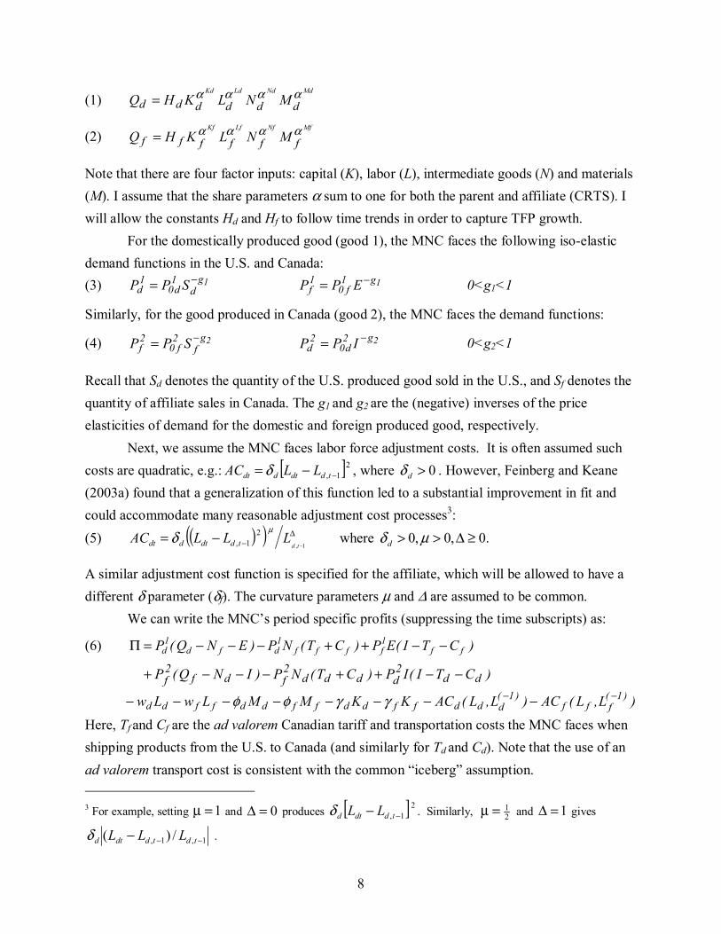
Note that there are four factor inputs: capital (K), labor (L), intermediate goods (N) and materials (M). I assume that the share parameters α sum to one for both the parent and affiliate (CRTS). I will allow the constants Hd and Hf to follow time trends in order to capture TFP growth.

For the domestically produced good (good 1), the MNC faces the following iso-elastic demand functions in the U.S. and Canada: (3) 1g

d1d0

1d SPP −= 1g1

f01f EPP −= 0<g1<1

Similarly, for the good produced in Canada (good 2), the MNC faces the demand functions:

(4) 2gf

2f0

2f SPP −= 2g2

d02

d IPP −= 0<g2<1

Recall that Sd denotes the quantity of the U.S. produced good sold in the U.S., and Sf denotes the quantity of affiliate sales in Canada. The g1 and g2 are the (negative) inverses of the price elasticities of demand for the domestic and foreign produced good, respectively.

Next, we assume the MNC faces labor force adjustment costs. It is often assumed such costs are quadratic, e.g.: [ ]2

1, −−= tddtddt LLAC δ , where 0>dδ . However, Feinberg and Keane (2003a) found that a generalization of this function led to a substantial improvement in fit and could accommodate many reasonable adjustment cost processes3: (5) ( )( ) ∆

− −−=

1,

21, td

LLLAC tddtddt

µδ where .0,0,0 ≥∆>> µδ d

A similar adjustment cost function is specified for the affiliate, which will be allowed to have a different δ parameter (δf). The curvature parameters µ and ∆ are assumed to be common.

We can write the MNC’s period specific profits (suppressing the time subscripts) as:

(6) )CTI(EP)CT(NP)ENQ(P ff1ffff

1dfd

1d −−++−−−=Π

)CTI(IP)CT(NP)INQ(P dd2dddd

2fdf

2f −−++−−−+

)L,L(AC)L,L(ACKKMMLwLw )1(fff

)1(dddffddffddffdd

−− −−−−−−−− γγφφ

Here, Tf and Cf are the ad valorem Canadian tariff and transportation costs the MNC faces when shipping products from the U.S. to Canada (and similarly for Td and Cd). Note that the use of an ad valorem transport cost is consistent with the common “iceberg” assumption. 3 For example, setting 1=µ and 0=∆ produces [ ]2

1, −− tddtd LLδ . Similarly, 21=µ and 1=∆ gives

1,1, /)( −−− tdtddtd LLLδ .

9

The exchange rate enters (6) implicitly because Canadian affiliate costs and revenues are converted into U.S. dollars using the nominal exchange rate. Thus, the MNC cares about U.S. dollar profits (and hence U.S. dollar output and input prices). wd and wf are the domestic and foreign real wage rates respectively, and φd and φf are the domestic and foreign materials prices. γ is the price of capital, which we assume is equal for the parent and the affiliate (γd = γf).

The MNC’s problem is to maximize the expected present value of profits in real U.S. dollars ∑ Π

∞

=+

1ττ

τβ tE by choice of eight control variables { }ft,ft,ft,ft,dt,dt,dt,dt NKMLNKML . The solution to this problem will generate shadow prices on intermediates shipped from the parent to affiliate and vice-versa.

Finally, recall assumption 8, that the rate of profit, defined as R=Π/γK, is equalized (in expectation) across firms. This can be justified by assuming a world where capitalists (as residual claimants) decide how to allocate capital across industries (or varieties of differentiated products) based on expected profit rates. In equilibrium, the profit rate will be equalized across industries (as entry reduces R). The equilibrium R will be positive if there is a fixed cost of entry that is proportional to size of the capital stock.

The virtue of assuming a particular profit rate is that one can back out the payments to capital from data on total revenues and payments to the other factors (rather than using PPE data).4 Thus, I treat the profit rate R as an unknown parameter to be estimated. I discuss the intuition for its identification in section IV.3.B.

II.3. Solution of the Firm’s Problem and Derivation of the Estimable FOCs We can express the FOCs more compactly if we first define:

A=

−−

+−−−)(

)()(1

11

ENQPCTNPENQP

fdd

fffdfdd =

+−

dd

fffddd

SPCTNPSP

1

11 )(

4 The procedure works as follows. Denote domestic revenue by RD, domestic costs by CD* and domestic costs excluding capital costs by CD1. These quantities are given by:

)EP)(CT1(NPSPRD 1ffff

1dd

1d −−++=

dddd2fdddddd

* AC)CT1(NPMKLwCD ++++++= φγ

dd KCD1CD γ−≡ Now, let RK denote the fraction of operating profit that is pure profit, leaving (1-RK) as the fraction that is the payment to capital. This gives Πd = RK ⋅ [RD-CD1] and thus: ]1CDRD[)R1(K Kdd −⋅−=γ Thus, the rate of profit for domestic operations is R = Πd / γdKd = RK/(1-RK). We treat R as a common parameter across firms and countries that we estimate (we also assume it is equal for the parent and the affiliate). That is, for the affiliate we have the analogous equation:

]1CFRF[)R1(K Kff −⋅−=γ

10

B=

−−

+−−−)(

)()(2

22

INQPCTNPINQP

dff

dddfdff =

+−

ff

dddfff

SPCTNPSP

2

22 )(

and express the adjustment cost term in the FOC for domestic labor (Ld ) as E(FD), where: FD = ∆µµ 1t,d1t,ddt

121t,ddt L)LL())LL(( −−

−− −−∂

- ∆µβµ dtdt1dt12

dt1dt L)LL())LL(( −− +−

+ - 1dtdt1dt

2dt1dt L)LL())LL(( +

++ −− ∆µ∆β

The adjustment cost term in the FOC for Canadian labor (Lf ) is E(FF), where FF is defined

similarly.

The first order conditions for parent factor inputs and parent’s exports to Canada are then:

0)FD(Ew)Ag1(:L dd

d1d

1Ld

d LQP

=−−

−α

0)Ag1(:K dd

d1d

1Kd

d KQP

=−

− γα

0)Ag1(:M dd

d1d

1Md

d MQP

=−

− φα

0P)CT1(BPg)Ag1(:N 2fdd

2f2

d

d1d

1Nd

d NQP

=++−+

−α

0P)Ag1()CT1(P)g1(:E 1d1ff

1f1 =−−−−−

For the affiliate, the first order conditions for Lf, Kf, Mf, Nf and I are similar. Note that the FOC for Nd, intermediates shipped from the affiliate to the parent, equates

the marginal revenue product from increasing the input of Nd in domestic production to the effective cost of importing Nd. The effective cost (or shadow price) can be written 2

2 )1( fPBg− .)( 2

fdd PCT ++ The first term is the marginal revenue from selling Nd in Canada. The component g2BPf

2 arises because the affiliate has market power. The second term is the tariff and transport cost, which is based on the “transfer price” 2

fP . Thus, I assume that the transfer price is equal to price that the firm charges third parties in Canada.5 Note that the shadow price is a 5 MNCs must set transfer prices for accounting purposes. It enables them to allocate profits to different countries for

tax purposes, and it enables then to calculate tariffs. I assume that the transfer price is equal to 2fP because both the

U.S. and Canadian revenue services require a “third party standard” whereby the transfer price should be set equal to the price charged to unaffiliated buyers. Canada has lower tax rates on manufacturing than the U.S., so there is an incentive to manipulate the transfer price to shift profits to Canada. However, Eden (1998) finds no evidence that transfer price manipulation is significant in eth U.S.-Canada context. Given that the tax differential is small and enforcement is relatively strict, it may be easier to transfer profits using licensing fees on intangibles.

11

completely separate quantity from the transfer price, since obviously it is not optimal for the affiliate to charge the parent the same price it charges third parties.

Since prices and quantities are not separately observed, one cannot take these FOCs directly to the data. They must first be manipulated to obtain estimable equations that contain only observed quantities and unknown model parameters. First, by multiplying each first order condition by the associated control variable, we obtain: 0L)FD(ELw)QP)(Ag1(:L ddddd

1d1

Ldd =−−− δα

0K)QP)(Ag1(:K ddd1

d1Kd

d =γ−−α

(7) 0M)QP)(Ag1(:M dd1

d1Md

d =φ−−α

0)NP)(CT1(B)NP(g)QP)(Ag1(:N d2fddd

2f2d

1d1

Ndd =++−+−α

0)EP)(Ag1()CT1)(EP)(g1(:E 1d1ff

1f1 =−−−−−

In the FOC for E, the quantity EPd1 is not observable.6 However, one can exploit the fact that:

)EP( 1d = )EP( 1

f1f

1d

P

P

= )EP( 1

f

1g

1f

d1d

1f0

1d0

EP

SP

P

P⋅

−

to express the FOC for E in terms of observable quantities and the demand function intercepts ( )1

010 fd PP , which are treated as unknown parameters, as follows:

(8) E: 0)EP()Ag1()CT1)(EP)(g1( 1f

1g

1f

d1d

1f0

1d0

1ff1f1 EP

SP

P

P=⋅

−−−−−

−

Similarly, in the FOCs for the factor inputs, the quantity )QP( d

1d is also not observed. We

can rewrite this quantity as ( ) )EP(PPNPSPQP 1f

1f

1df

1dd

1dd

1d ++= but, again, EP1

d is not

observed. I therefore repeat the same type of substitution to obtain, for domestic labor:

(9) 0L)FD(ELw)EP(NPSP)Ag1(:L dddd1f

g

1f

d1d

1f0

1d0

f1dd

1d1

Ldd

1

EP

SP

P

P=−−

++−

−

δα

The FOCs for Kd, Md and Nd, and for the affiliate, are obtained similarly.

6 Note: Pd

1E is the physical quantity of exports times their domestic (not foreign) price – an object we cannot construct since we do not observe prices and quantities separately

12

III. Stochastic Specification The model contains eight parameters (R, β, δd, δf, µ, ∆, Hd and Hf) that are common

across firms. The model also contains eight technology parameters (αKd, αLd, αNd, αMd, αKf, αLf, αNf, αMf) and six demand function parameters (g1, 1

d0P , 1f0P , g2, 2

d0P and 2f0P ) that are allowed to

be heterogeneous both across firms and within firms over time. Given CRTS, two of the Cobb-Douglas share parameters (α) are determined by the other six. Thus, there are 12 fundamental parameters that can vary independently. In addition, the two unobserved expectation terms E(FD) and E(FF) that appear in the FOCs for U.S. and Canadian labor must also be dealt with. III.1. Production Function Parameters

Allowing the Cobb-Douglas share parameters to be stochastic, while also imposing that they are positive and sum to one (CRTS), is challenging. To impose these constraints, I use a logistic-type transformation, treating the share parameters as analogous to choice probabilities in a multinomial logit (MNL) model. For instance, for the domestic labor share parameter, we have, suppressing firm and time subscripts:

KdR

MdR

LdR

LdRLd

ααααα

+++=

1)10( { }

{ } { } { }KdKdMdMdLdLd

LdLd

xGxGxGxG

εαεαεαεα

+++++++=

1

where G(⋅)>0 is a positive function, the vector xit includes all firm characteristics that shift the share parameters, and Ldα is a corresponding vector of parameters.

The expressions for αKd and αMd are similar. Note the expression for αNd is:

(11) { } { } { }KdKdMdMdLdLdNd

xGxGxG εαεαεαα

++++++=

11

So Ndα plays the role of the “base alternative” in a multinomial logit model. This specification insures that, given any values for the xit and any values for the stochastic terms εit, the Cobb-Douglas share parameters are guaranteed to be positive and sum to 1.

Note that in (10) the quantities LdRα , Md

Rα and KdRα are simply latent variables that map

into the firm specific share parameters. If we specify that G(a) =exp(a) and that the ε are normal we obtain a specification where Ld

Rα , MdRα and Kd

Rα are log normal. Then, for example, the stochastic term Ld

Rα would be given by: LdLdLd

R x εαα +=ln Ldε ~ ),0(N 2Ldσ

and similar equations could be specified for MdRα , Kd

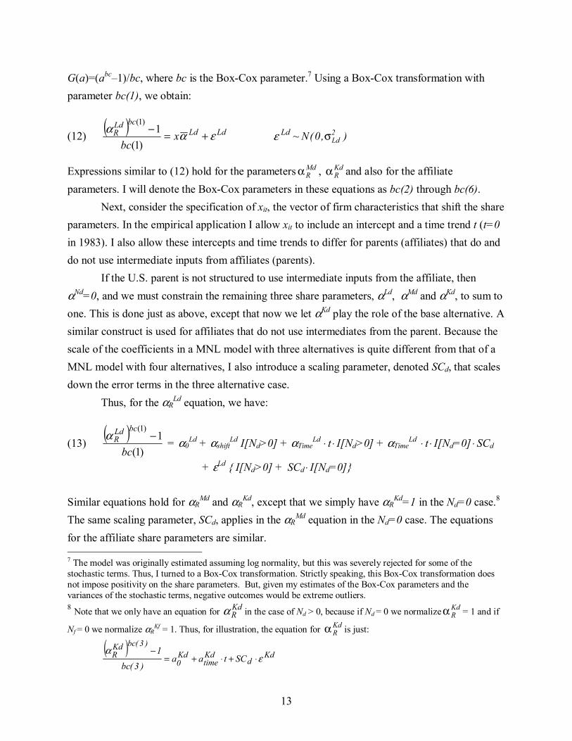
Rα . We can easily generalize log normality by using a Box-Cox transformation, given by

13

G(a)=(abc–1)/bc, where bc is the Box-Cox parameter.7 Using a Box-Cox transformation with parameter bc(1), we obtain:

(12) ( ) LdLdbcLd

R xbc

εαα +=−)1(

1)1(

Ldε ~ ),0(N 2Ldσ

Expressions similar to (12) hold for the parameters MdRα , Kd

Rα and also for the affiliate parameters. I will denote the Box-Cox parameters in these equations as bc(2) through bc(6).

Next, consider the specification of xit, the vector of firm characteristics that shift the share parameters. In the empirical application I allow xit to include an intercept and a time trend t (t=0 in 1983). I also allow these intercepts and time trends to differ for parents (affiliates) that do and do not use intermediate inputs from affiliates (parents).

If the U.S. parent is not structured to use intermediate inputs from the affiliate, then αNd=0, and we must constrain the remaining three share parameters, αLd, αMd and αKd, to sum to one. This is done just as above, except that now we let αKd play the role of the base alternative. A similar construct is used for affiliates that do not use intermediates from the parent. Because the scale of the coefficients in a MNL model with three alternatives is quite different from that of a MNL model with four alternatives, I also introduce a scaling parameter, denoted SCd, that scales down the error terms in the three alternative case.

Thus, for the αRLd equation, we have:

(13) ( )

)1(1

)1(

bc

bcLdR −α

= α0Ld + αshift

Ld I[Nd>0] + αTimeLd ⋅ t⋅ I[Nd>0] + αTime

Ld ⋅ t⋅ I[Nd=0]⋅ SCd

+ εLd { I[Nd>0] + SCd⋅ I[Nd=0]} Similar equations hold for αR

Md and αRKd, except that we simply have αR

Kd=1 in the Nd=0 case.8 The same scaling parameter, SCd, applies in the αR

Md equation in the Nd=0 case. The equations for the affiliate share parameters are similar. 7 The model was originally estimated assuming log normality, but this was severely rejected for some of the stochastic terms. Thus, I turned to a Box-Cox transformation. Strictly speaking, this Box-Cox transformation does not impose positivity on the share parameters. But, given my estimates of the Box-Cox parameters and the variances of the stochastic terms, negative outcomes would be extreme outliers. 8 Note that we only have an equation for Kd

Rα in the case of Nd > 0, because if Nd = 0 we normalize KdRα = 1 and if

Nf = 0 we normalize αRKf = 1. Thus, for illustration, the equation for Kd

Rα is just:

( ) Kdd

Kdtime

Kd0

)3(bcKdR SCtaa

)3(bc

1ε

α⋅+⋅+=

−

14

Turning to the correlations of the ε, I specify that:

(14) ( )′NdMdLd εεε ~ ( )dN Σ,0 ,

where Σd is unrestricted. Similarly, for affiliates, Σf is unrestricted. But, in order to conserve on parameters, I do not allow for covariances between the parent and affiliate share parameters.9 Finally, consider the TFP parameters Hd and Hf in equations (1) and (2). Since we do not observe output prices and quantities separately, we cannot identify the scale of the H (either absolutely or for the affiliate relative to the parent). However, we can identify technical progress. Thus I normalize Hd = Hf = 1 at t=0 (1983) and let each have a time trend:

(15) Hjt = (1 + hj )t for j=d,f.

A specification with equal time trends could not be rejected, so I set hd = hf = h.

III.2. Demand Function Parameters Now I turn to the stochastic specification for the demand function parameters. For the

inverse price elasticity of demand, or market power, parameter g1 we have: ( )

1,110

71

)7(1

)16( gshift1,time

bc0]·I[Ndgtgg

bcg

ε+>+⋅+=−

A similar equation holds for g2, and the Box–Cox parameter in that equation is bc(8).

For the demand function intercepts for good 1 in the domestic market, I specify:10

101

,01

0,0

)9(10

)9(1)(

)17( dP1 shift0d,timedd

bcd 0]·I[NdPtPPbc

P ε+>+⋅+=−

Similar equations hold for 20 fP , 1

0 fP and 20dP , and the Box-Cox parameters in these equations are

denoted by bc(10), bc(11) and bc(12), respectively. Preliminary results suggested that cross correlations between the three groups of parameters (technology, price elasticities, and demand function intercepts), were not important. Allowing for such correlations leads to a severe proliferation of parameters. Thus, I assume 1gε and 2gε are independent of other stochastic terms. I let the ),,,(

2d0

1f0

2f0

1d0 PPPP εεεε vector be correlated

within itself with covariance matrix ΣP, but it is independent of the other stochastic terms.

9 Interpretation of the Σd and Σf terms is rather subtle. The logistic transformation already incorporates the negative correlation among the share parameters that is generated by the CRTS assumption. If Σd = I, we have an “IIA” setup, where if one domestic share parameter increases, the other share parameters decrease proportionately. The correlations in Σd and Σf allow firms to depart from this IIA situation. For example, if Σd

12 is very large, then we get a pattern where firms with large domestic labor shares also have large domestic materials shares. 10 Technically, we should impose that g1 and g2 are positive and less than 1, and that the Po terms are positive. Equations (16)-(17) do not impose these constraints. But, given the estimates, violations would be extreme outliers.

15

III.3 Labor Force Adjustment Cost Parameters Recall that labor force adjustment costs are given by equation (5). The parameters δd and

δf are allowed to vary across firms as follows: (18) { }]0N[Itwexp dtdddtd0,1ddt >⋅+⋅++= δδδδδ { }]0N[Itwexp ftffftf0,1fft >⋅+⋅++= δδδδδ As with the other structural parameters, I allow for the possibility that adjustment costs vary over time, and between firms that do and do not have intra-firm flows. I also allow the δ to be functions of the wage rate, since search and severance costs for high skilled labor are higher. III.4. Serial Correlation

I model serial correlation of the errors for each firm using a random effects structure. For example, for the stochastic part of the parent labor share parameter εLd we have:

)()()( itLdiLditLd νµε += for t=1,…Ti

and similarly for the other eleven parameters. Let µi ∼ N(0, Σµ) denote the 12×1 vector of random effects for firm i, and let νit ∼ N(0, Σν) denote the 12×1 vector of firm/time specific error components. Then, Vt ≡ Var(εit) = Σµ + Σν and Ct-j, t ≡ Cov(εit, εi,t-j) = Σµ . Note that Σµ and Σν each contain 78 unique elements, but these are restricted as described earlier. For instance, the non-zero elements of Σµ + Σν consist entirely of elements of Pfd , ΣΣΣ and along with 2

1gσ and 22gσ . Other cross-correlations are set to zero. Defining ),....,(

iiT1ii εεε = we have:

(19)

=

ii TT1

212

1

i

VC

VCV

)(Var

LL

OMε

So far, I have only considered the most general case where a firm has all 4 potential trade flows. If a firm has Ndt=0 (or Nft=0) at time t, then there is no value for εKd(it) (or εKf(it)). Similarly, if Et=0, there is no value for )it(1

f0P , and if It=0 there is no value for )it(2d0P . Additionally, some

firms are not observed for consecutive years. In such cases Var(εi) is collapsed in the obvious way (by removing the relevant rows and columns). III.5. Unobserved Expectation Terms I deal with the unobserved expectation term E(FD)Ld in (9) by invoking a rational expectations assumption:

(20) ditdititdititt LFDL)FD(E η−=

where ditη is a forecast error assumed orthogonal to all information available at time t. A similar

expression is specified for E(FF)Lf. The distributions of ditη and ηit

f are discussed Section IV.

16

IV. Estimation using the SML Based on FOCs Approach IV. 1. Motivation If we substituting (20) into (9), we see that the FOC for domestic labor will contain five firm specific stochastic terms (αit

Ld, g1it, 1d0P , 1

f0P and ditη ) that enter non-linearly. Hence, it is not

possible to express the equation as a moment condition with a single additive error term.11 The same is true of all 12 FOCs of the model, since they all involve multiple stochastic terms that enter nonlinearly. Thus, GMM estimation is infeasible. One alternative to GMM would be a full information ML approach (FIML). This would require the econometrician to specify how firms form expectations of future labor inputs. This in turn would require that one specify how firms forecast future demand and technology shocks, tariffs, exchange rates, etc. This means completely specifying the stochastic processes for all these forcing variables. Thus, a FIML approach would force a researcher to make assumptions about a wide range of issues that go well beyond the nature of the firm’s technology and the structure of demand. The SML based on FOCs approach is another alternative. The fact that multiple stochastic terms enter the FOCs in (8)-(9) in a highly nonlinear way creates no problems for this approach. SML based on FOCs can be thought of as a compromise between FIML and GMM. As in a FIML approach, the econometrician must specify parametric distributions for the demand and technology shocks. But, rather than specify stochastic processes for all the forcing variables (e.g., tariffs, wages, etc.), one simply substitutes realizations of the t+1 labor demand terms for their expectations, as in a typical GMM approach. However, the SML based on FOCs approach requires that we specify a distribution for the forecast errors ηit

d and ηitf.

In terms of what one can do with the model once it is estimated, SML based on FOCs also represents a compromise between FIML and GMM approach. Since we estimate the complete distribution of technology and demand parameters for the MNCs, we can do steady state simulations of the responses of the whole population of firms to changes in the tariffs and other features of the environment.12 But, since we do not model the evolution over time of all the forcing processes, we cannot simulate transition paths to a new steady state.13

11 Even if we could linearize (9), finding valid instruments is difficult. Usual candidates like input prices would be correlated with firm specific technology parameters if technology changes over time in response to price changes. 12 Note that, even if GMM estimation were feasible for our model, it would not be adequate for this purpose. The usual argument for GMM over ML is that one avoids making distributional assumptions on the stochastic terms, and thereby obtains more robust estimates of model parameters. But we must estimate the distributions of the firm specific parameters if we want to simulate the response of the population of firms to changes in the environment. 13 It is worth emphasizing that the key difficulty in estimation arises not from dynamics, but rather because multiple stochastic terms enter the FOCs. This problem would be present in a static model without labor adjustment costs.

17

IV.2 The Stochastic Process for Forecast Errors

Without loss of generality I rewrite (20), the equation for forecast errors, as follows:

(21) *)( dtdtdititditit LFDLFDE ησ+=

where *dtη is standard normal. Of course, there is no reason one could not specify a more flexible

parametric distribution. For instance, Feinberg and Keane (2003a) estimated a generalized version of this model where *

dtη was assumed to be normal subject to a Box-Cox transform. But the estimated Box-Cox parameter was extremely close to one, implying that the distributions of the forecast errors are indeed well described by normality in this model.

It is plausible that that σdt, the standard deviation of the labor adjustment cost forecast error, will be increasing in Ldit, so I write:

(22) { }dt10ddt Lexp ττσ += , { }ft10fft Lexp τσ τ +=

Regarding serial correlation, I assume that the forecast errors are independent over time, as implied by rational expectations. But I allow parent and affiliate forecast errors to be correlated within a period, as must be the case if their production processes are integrated, or if they face common shocks. Thus, I let ( )′fd ηη ∼ N(0 , Ση). I also let Ση = CC′ , where C is the lower

triangular Cholesky decomposition

2212

11

CC0C

. Finally, let τ = (τd0, τf0, τ1).

IV.3. Construction of the Simulated Likelihood Function IV.3.A. Overview Let θ denote the vector of all model parameters. It includes values for the common (or non-stochastic) parameters of the model, which are R, β, δd, δf, µ, ∆, τ and h, as well as the parameters of the joint distribution of the 12 firm specific stochastic terms (see section III). Given a value of θ, simulation of a firm’s likelihood contribution involves the following steps:

Step 1: Take a draw from the joint distribution of the forecast errors, ηd and η f.

Step 2: Use the ten first FOCs for Ld, Kd, Md, Nd, Lf, Kf, Mf, Nf, E, and I (see eqns. 8-9), and the production functions (1) and (2) as a system of 12 equations to solve for the 12 stochastic terms that rationalize the firm’s behavior in each time period. Step 3: Calculate the joint density of the stochastic terms, using the multivariate normal distribution with covariance matrix given by (19). Step 4: Multiply by the Jacobian to obtain the data density. Repeating this process at independent draws for ηd and η f, and averaging the data densities so obtained, we obtain a simulation consistent estimate of the likelihood contribution for the firm.

18

While this process is conceptually straightforward, some aspects of the computation require new simulation methods that will be developed below. In step 2, solving the system of 12 nonlinear equations for the 12 stochastic terms in the model is cumbersome. But it is not computationally difficult. However, there are some draws for ηd and η f in step 1 such that the system in step 2 has no solution. That is, there are regions of the space of forecast errors such that firm behavior is not rationalizable, and the boundaries of these regions depend on θ. Thus, in order to simulate the likelihood, it is not advisable to naively take draws from the unconditional distribution of ηd and η f in step 1. We have a model where all the stochastic terms are continuous, yet they must fall in certain sub-regions of a high dimensional space in order for firm behavior to be rationalizable by the model. As a result, a high dimensional integral must be evaluated to construct the joint density of a firm’s stochastic terms. Section IV.3.E presents a recursive importance sampling algorithm that can deal effectively with this integration problem. The algorithm is the discrete/continuous analogue of the GHK algorithm. The second problem is that the Jacobian required for step 4 is analytically intractable. But in sections IV.3.C and IV.3.E I show how it can be approximated using simulation methods and numerical derivatives. IV.3.B. Solving for the Error Terms (and Identification of the Model Parameters) Solving the system of 12 nonlinear equations for the 12 stochastic parameters in the model is cumbersome. I relegate the details to Appendix 1, but here I give an overview of the process. Understanding this process is important both for understanding the simulation methods that are developed later, as well as for understanding how the model parameters are identified. In this section, assume for the moment that we have already obtained a valid draw for the forecast errors, ηd and η f, and that we seek to solve for the remaining 12 stochastic terms of the model. The market power parameters g1 and g2 are identified by simple markup relationships (i.e., Lerner conditions), which we can construct using data on sales revenues and costs. These relationships are modified slightly to account for labor force adjustment costs, and also for the complication that the MNC has an incentive to hold down prices of final goods it ships intra-firm as intermediates (in order to avoid tariff costs). (See equation A1.11). The U.S./Canadian price ratios for goods 1 and 2, denoted PR1 and PR2, are determined by the tariff and transport cost wedge, again modified by the incentive to hold down prices of intra-firm intermediates. Since the strength of this incentive depends only on g1 and g2, we can solve for PR1 and PR2 once g1 and g2 are obtained (see equation A1.12). Also, given g1 and g2, the Cobb-Douglas share parameters are identified by cost shares of modified revenues (see equation A1.13). Finally, given g1 and PR1, we can infer the ratio of the U.S. to Canadian demand function intercepts for good 1 (i.e., P0d

1/P0f1) by observing the ratio of U.S. to Canadian sales for good 1.

19

Similarly, by comparing affiliate sales in Canada vs. imports to the U.S., we can infer the ratio of domestic to foreign demand function intercepts for good 2 (i.e., P0f

2/P0d2).

Thus, without separate data on prices and quantities (except wages and employment, which we need only to identify the labor force adjustment cost function), we can identify the market power parameters, the Cobb-Douglas share parameters, and the ratios of the demand function intercepts for goods 1 and 2. To identify the levels of the demand intercepts, we need capital and materials price indices. Then, we can construct real capital and materials inputs, and use the production functions (1)-(2) as additional equations to determine quantities of output.

The preceding discussion assumes that we are solving for the stochastic terms at a given value of θ, which means at a given value of the profit rate R. Knowledge of R enables us to construct total costs, which enables us in turn to construct g1 and g2 using markups inferred from revenue and cost data. A key issue is how R is identified. As I show in Appendix 2, the model implies a relation g/(1-g) = αK ⋅ R between market power and capital share. Thus, if the profit rate is low (high), there is a strong (weak) tendency for firms with more market power to also have larger capital shares, so that profits accrue to a larger (smaller) stock of capital. In other words, the larger is R, the greater the extent to which firms with larger capital shares also have larger markups (i.e., face more inelastic demand).

Thus, to the extent that firms with larger capital shares act as if they face less elastic demand (in terms of how they respond to changes in the forcing variables), we will infer a higher value of R. At first this may seem like a strange argument for identification, since the capital share is not observed. However, given the assumption that R is equal for all firms, the capital share is perfectly negatively correlated with the sum of the labor, materials and intermediate shares. Thus, the greater the extent to which firms with larger labor plus materials plus intermediate shares act as if they face more elastic demand, the larger the implied R.14

Having solved for all the firm specific parameters, we use the equations of the stochastic specification (see section III) to construct the vector of error terms for the firm. Let εit denote the vector of (up to) 12 error terms for firm i in period t (or, as few as 8 if Nd = Nf = E = I = 0):

εit ≡ ( εitLd, εit

Md, εitNd, εit

Lf, εitMf, εit

Nf, εitg1, εit

g2, ),,,2d0

1f0

2f0

1d0 P

itP

itP

itP

it εεεε Finally, I construct the joint multivariate normal density of the error vector for firm i, which I denote by εi ≡ (εi1 , … , εiT(i)), where T(i) is the number of time periods that firm i is observed, using the covariance structure given by equation (19).

14 Appendix 2 also gives an intuitive explanation of how the time trends in TFP (h) and in the demand function intercepts (the P0) are separately identified. Briefly, to the extent that growth is more than proportionately slower for firms with more market power, it implies that growth is induced by TFP rather than growth in demand.

20

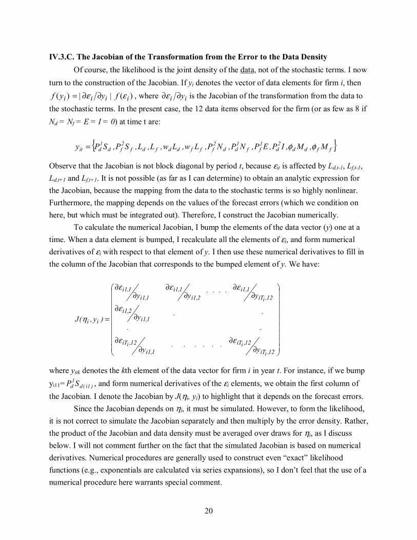
IV.3.C. The Jacobian of the Transformation from the Error to the Data Density Of course, the likelihood is the joint density of the data, not of the stochastic terms. I now

turn to the construction of the Jacobian. If yi denotes the vector of data elements for firm i, then )(||)( iiii fyyf εε ∂∂= , where ii y∂∂ε is the Jacobian of the transformation from the data to

the stochastic terms. In the present case, the 12 data items observed for the firm (or as few as 8 if Nd = Nf = E = I = 0) at time t are:

{ }ffdd

2d

1ff

1dd

2fffddfdf

2fd

1dit M,M,IP,EP,NP,NP,Lw,Lw,L,L,SP,SPy φφ=

Observe that the Jacobian is not block diagonal by period t, because εit is affected by Ld,t-1, Lf,t-1, Ld,t+1 and Lf,t+1. It is not possible (as far as I can determine) to obtain an analytic expression for the Jacobian, because the mapping from the data to the stochastic terms is so highly nonlinear. Furthermore, the mapping depends on the values of the forecast errors (which we condition on here, but which must be integrated out). Therefore, I construct the Jacobian numerically.

To calculate the numerical Jacobian, I bump the elements of the data vector (y) one at a time. When a data element is bumped, I recalculate all the elements of εi, and form numerical derivatives of εi with respect to that element of y. I then use these numerical derivatives to fill in the column of the Jacobian that corresponds to the bumped element of y. We have:

∂∂

⋅⋅⋅⋅⋅⋅∂∂

⋅⋅

⋅∂∂

∂∂⋅⋅⋅⋅∂

∂∂

∂

=

12,iT12,iT

1,1i12,iT

1,1i2,1i

12,iT1,1i

2,1i1,1i

1,1i1,1i

ii

i

ii

i

yy

.y

yyy

)y,(J

εε

ε

εεε

η

where yitk denotes the kth element of the data vector for firm i in year t. For instance, if we bump yi11= )1i(d

1d SP , and form numerical derivatives of the εi elements, we obtain the first column of

the Jacobian. I denote the Jacobian by J(ηi, yi) to highlight that it depends on the forecast errors. Since the Jacobian depends on ηi, it must be simulated. However, to form the likelihood, it is not correct to simulate the Jacobian separately and then multiply by the error density. Rather, the product of the Jacobian and data density must be averaged over draws for ηi, as I discuss below. I will not comment further on the fact that the simulated Jacobian is based on numerical derivatives. Numerical procedures are generally used to construct even “exact” likelihood functions (e.g., exponentials are calculated via series expansions), so I don’t feel that the use of a numerical procedure here warrants special comment.

21

IV.3.D. Simulating the Likelihood Function: Naïve Approach I form the likelihood by integrating the data density over the forecast error distribution:

L iiiiN

1id)f(),|y(f)(

i

ηηθηθη

Π ∫=

=

iiiiiiiiN

1id)y,(f)|)y,((f)y,(J

i

ηηθηεηη

Π ∫=

=

Here, ,),.....,,( fiiT

diiT

f1i

d1ii ηηηηη ≡ f(ηi) denotes the joint density of forecast errors for firm i, and

θ denotes the vector of model parameters. The notation εi (ηi , yi) emphasizes that the mapping

from the data to the stochastic terms for a firm depends on the vector of forecast errors ηi. Naively, one could simulate the likelihood function by taking iid draws from the

distribution of ηi. An important complication arises here, however. Firm behavior cannot be rationalized by any arbitrary values for the forecast errors. Conditional on a particular draw for (ηd, ηf ), firm behavior is only rationalizable if, when we solve the mapping from the data to the model parameters, we obtain 1>g1 > 0 , 1>g2 > 0, all technology parameters positive, and all demand shift parameters positive. But this will not be the case for all possible (ηd, ηf ) draws.

In Appendix 1, I derive the following equation relating g1 and the forecasts E(FD)Ld :

(23) B)NP(L)FD(ECDRD]AYE[g d2fBVI

)L)FF(ECFRF(ddBVI

)NP)(NP(AB1

ffd2ff

1d δδ −−

+−−=−

In the data, the term BVI/)NP)(NP(ABAYE d

2ff

1d− is always positive.15 So, the right-hand

side of (23) must be positive in order for g1 to be positive. But if the forecasted adjustment costs E(FD) = FD - ηd or E(FF) = FF - η f are too large, the right-hand side will be driven negative. Thus, observed firm behavior implies bounds on the forecast errors. I derive the exact bounds on (ηd, η f ) in Appendix 3.

For any draw (ηd, η f ) that does not satisfy the bounds, no values of the firm specific parameters can rationalize firm behavior. Let BDi denote the region of the space of forecast errors such that behavior of firm i is rationalizable. Then, we can rewrite the likelihood as:

1iBD

iTiiiiiBD

N

1id...d)f(...)f()|)y,((f)y,(J..........)

iiTiiT

i

1i1i

ηηηηθηεηθηη

Π ∫∫∈∈=

=( i1iTiL

15 A and B are usually close to 1. Therefore, AYE is close to sales of good 1, and BVI is close to sales of good 2 (see Appendix 1 for definitions). Thus, the second term includes (Pf

2Nd / BVI ), a number < 1, times Pd1Nf , which is just

one component of sales of good 1. So the whole term in brackets is roughly sales of good 1 minus a fraction thereof.

22

1iiTiiiiiN

1id...d)f(.......)f(]BD[I.......]BD[I)|)y,((f)y,(J... i

iiT1i

ηηηηηηθηεηηη

Π i1iTi1i1iTiT iii∫ ∈∈∫==

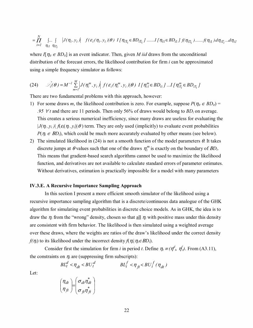
where I[ηit ∈ BDit] is an event indicator. Then, given M iid draws from the unconditional distribution of the forecast errors, the likelihood contribution for firm i can be approximated using a simple frequency simulator as follows:

(24) ]BD[I...]BD[I)|)y,((f)y,(JM)(̂ iTm

iiTm1ii

mii

M

1mi

mi

1ii1i ∈∈∑=

=

− ηηθηεηθL

There are two fundamental problems with this approach, however: 1) For some draws m, the likelihood contribution is zero. For example, suppose P(ηit ∈ BDit) =

.95 ∀ t and there are 11 periods. Then only 56% of draws would belong to BDi on average. This creates a serious numerical inefficiency, since many draws are useless for evaluating the |J(ηi ,yi )| f(εi(ηi ,yi)|θ ) term. They are only used (implicitly) to evaluate event probabilities P(ηi ∈ ΒDi), which could be much more accurately evaluated by other means (see below).

2) The simulated likelihood in (24) is not a smooth function of the model parameters θ. It takes discrete jumps at θ values such that one of the draws m

iη is exactly on the boundary of ΒDi. This means that gradient-based search algorithms cannot be used to maximize the likelihood function, and derivatives are not available to calculate standard errors of parameter estimates. Without derivatives, estimation is practically impossible for a model with many parameters

IV.3.E. A Recursive Importance Sampling Approach

In this section I present a more efficient smooth simulator of the likelihood using a recursive importance sampling algorithm that is a discrete/continuous data analogue of the GHK algorithm for simulating event probabilities in discrete choice models. As in GHK, the idea is to draw the ηi from the “wrong” density, chosen so that all ηi with positive mass under this density are consistent with firm behavior. The likelihood is then simulated using a weighted average over these draws, where the weights are ratios of the draw’s likelihood under the correct density f(ηi) to its likelihood under the incorrect density f(ηi|ηi∈ΒDi).

Consider first the simulation for firm i in period t. Define ηt ≡ (ηdt, ηf

t). From (A3.11), the constraints on ηt are (suppressing firm subscripts):

dtdt

dt BUBL <<η )(BUBL dt

ftft

ft ηη <<

Let:

=

*ftft

*dtdt

ft

dt

ησ

ησηη

23

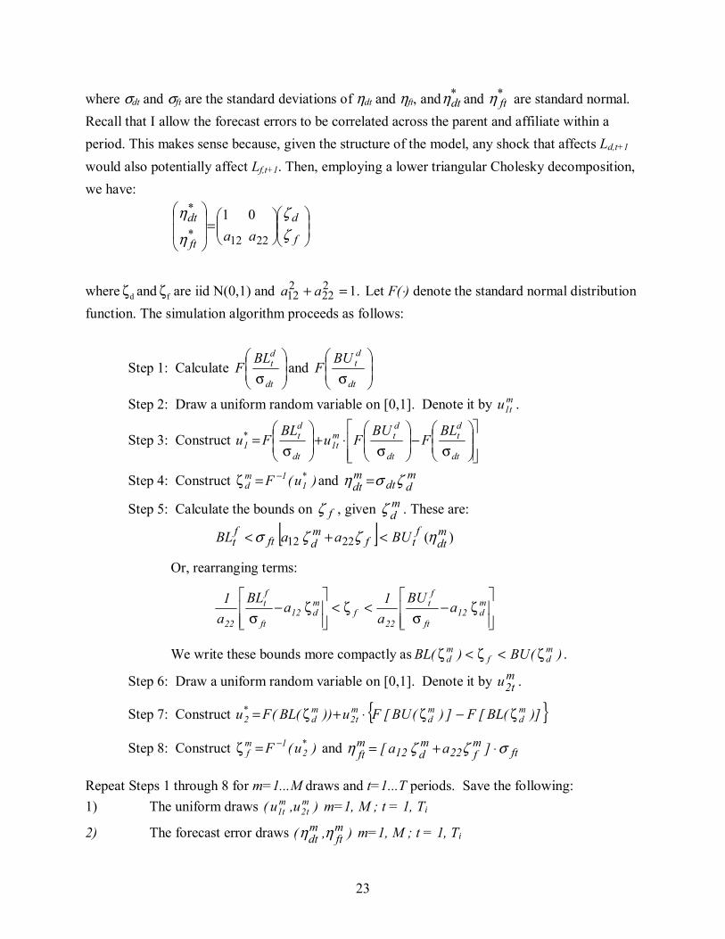
where σdt and σft are the standard deviations of ηdt and ηft, and *dtη and *

ftη are standard normal. Recall that I allow the forecast errors to be correlated across the parent and affiliate within a period. This makes sense because, given the structure of the model, any shock that affects Ld,t+1 would also potentially affect Lf,t+1. Then, employing a lower triangular Cholesky decomposition, we have:

=

f

d

ft

dtaa ζ

ζ

η

η

2212*

* 01

where dζ and fζ are iid N(0,1) and .12

22212 =+ aa Let F(⋅) denote the standard normal distribution

function. The simulation algorithm proceeds as follows:

Step 1: Calculate

σdt

dtBL

F and

σdt

dtBU

F

Step 2: Draw a uniform random variable on [0,1]. Denote it by mt1u .

Step 3: Construct

σ−

σ⋅+

σ=

dt

dt

dt

dtm

t1dt

dt*

1BL

FBU

FuBL

Fu

Step 4: Construct )u(F *1

1md

−=ζ and mddt

mdt ζση =

Step 5: Calculate the bounds on fζ , given mdζ . These are:

[ ] )(2212mdt

ftf

mdft

ft BUaaBL ηζζσ <+<

Or, rearranging terms:

ζ−

σ<ζ<

ζ−

σmd12

ft

ft

22f

md12

ft

ft

22a

BUa1a

BLa1

We write these bounds more compactly as )(BU)(BL mdf

md ζ<ζ<ζ .

Step 6: Draw a uniform random variable on [0,1]. Denote it by mt2u .

Step 7: Construct { })](BL[F])(BU[Fu))(BL(Fu md

md

mt2

md

*2 ζ−ζ⋅+ζ=

Step 8: Construct )u(F *2

1mf

−=ζ and ftmf22

md12

mft ]aa[ σζζη ⋅+=

Repeat Steps 1 through 8 for m=1...M draws and t=1...T periods. Save the following: 1) The uniform draws )u,u( m

t2mt1 m=1, M ; t = 1, Ti

2) The forecast error draws ),( mft

mdt ηη m=1, M ; t = 1, Ti

24

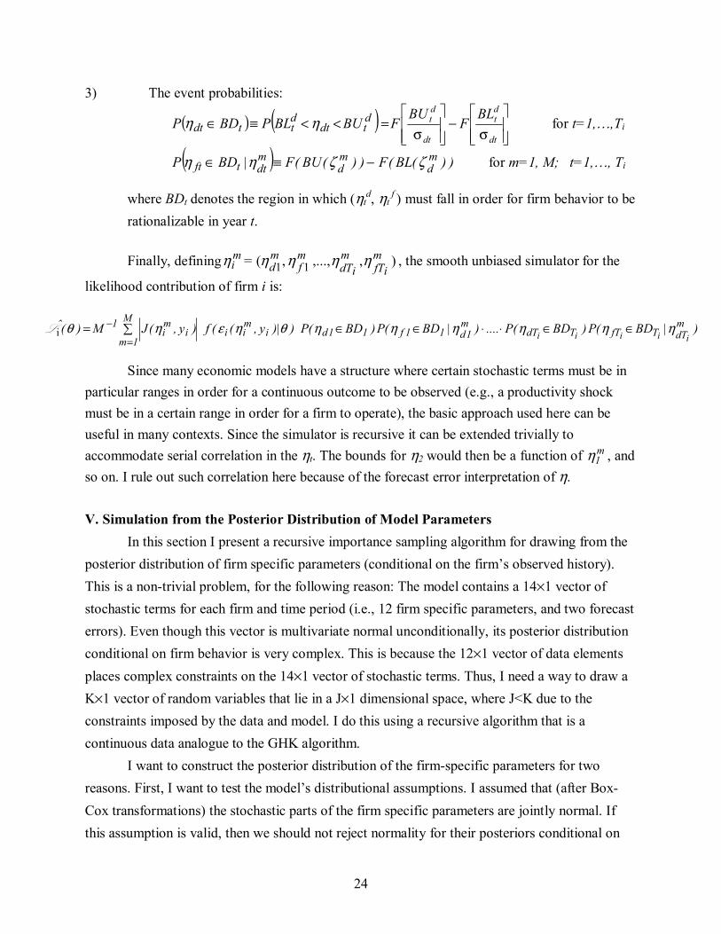
3) The event probabilities:

( ) ( )dtdt

dttdt BUBLPBDP <<≡∈ ηη

σ−

σ=

dt

dt

dt

dt BL

FBU

F for t=1,…,Ti

( ) ))(BL(F))(BU(F|BDP md

md

mdttft ζζηη −≡∈ for m=1, M; t=1,…, Ti

where BDt denotes the region in which (ηtd, ηt

f ) must fall in order for firm behavior to be

rationalizable in year t. Finally, defining m

iη = ),,...,,( 11m

ifTm

idTmf

md ηηηη , the smooth unbiased simulator for the

likelihood contribution of firm i is:

)|BD(P)BD(P....)|BD(P)BD(P)|)y,((f)y,(JM)(ˆ mdTTfTTdT

m1d11f11di

mii

M

1mi

mi

1iiiii ηηηηηηθηεηθ ∈∈⋅⋅∈∈∑=

=

−iL

Since many economic models have a structure where certain stochastic terms must be in

particular ranges in order for a continuous outcome to be observed (e.g., a productivity shock must be in a certain range in order for a firm to operate), the basic approach used here can be useful in many contexts. Since the simulator is recursive it can be extended trivially to accommodate serial correlation in the ηt. The bounds for η2 would then be a function of m

1η , and so on. I rule out such correlation here because of the forecast error interpretation of η. V. Simulation from the Posterior Distribution of Model Parameters

In this section I present a recursive importance sampling algorithm for drawing from the posterior distribution of firm specific parameters (conditional on the firm’s observed history). This is a non-trivial problem, for the following reason: The model contains a 14×1 vector of stochastic terms for each firm and time period (i.e., 12 firm specific parameters, and two forecast errors). Even though this vector is multivariate normal unconditionally, its posterior distribution conditional on firm behavior is very complex. This is because the 12×1 vector of data elements places complex constraints on the 14×1 vector of stochastic terms. Thus, I need a way to draw a K×1 vector of random variables that lie in a J×1 dimensional space, where J<K due to the constraints imposed by the data and model. I do this using a recursive algorithm that is a continuous data analogue to the GHK algorithm.

I want to construct the posterior distribution of the firm-specific parameters for two reasons. First, I want to test the model’s distributional assumptions. I assumed that (after Box-Cox transformations) the stochastic parts of the firm specific parameters are jointly normal. If this assumption is valid, then we should not reject normality for their posteriors conditional on

25

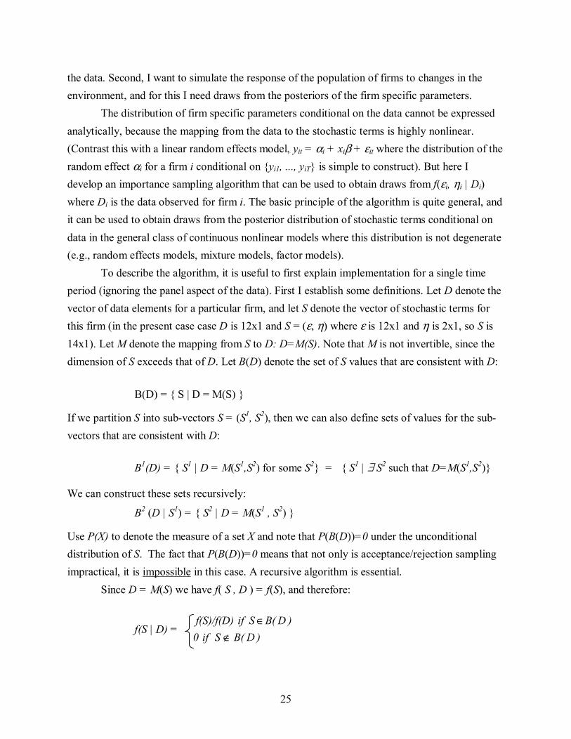
the data. Second, I want to simulate the response of the population of firms to changes in the environment, and for this I need draws from the posteriors of the firm specific parameters. The distribution of firm specific parameters conditional on the data cannot be expressed analytically, because the mapping from the data to the stochastic terms is highly nonlinear. (Contrast this with a linear random effects model, yit = αi + xiβ + εit where the distribution of the random effect αi for a firm i conditional on {yi1, ..., yiT} is simple to construct). But here I develop an importance sampling algorithm that can be used to obtain draws from f(εi, ηi | Di) where Di is the data observed for firm i. The basic principle of the algorithm is quite general, and it can be used to obtain draws from the posterior distribution of stochastic terms conditional on data in the general class of continuous nonlinear models where this distribution is not degenerate (e.g., random effects models, mixture models, factor models). To describe the algorithm, it is useful to first explain implementation for a single time period (ignoring the panel aspect of the data). First I establish some definitions. Let D denote the vector of data elements for a particular firm, and let S denote the vector of stochastic terms for this firm (in the present case case D is 12x1 and S = (ε, η) where ε is 12x1 and η is 2x1, so S is 14x1). Let M denote the mapping from S to D: D=M(S). Note that M is not invertible, since the dimension of S exceeds that of D. Let B(D) denote the set of S values that are consistent with D:

B(D) = { S | D = M(S) }

If we partition S into sub-vectors S = (S1, S2), then we can also define sets of values for the sub- vectors that are consistent with D: B1(D) = { S1 | D = M(S1,S2) for some S2} = { S1 | ∃ S2 such that D=M(S1,S2)} We can construct these sets recursively:

B2 (D | S1) = { S2 | D = M(S1 , S2) }

Use P(X) to denote the measure of a set X and note that P(B(D))=0 under the unconditional distribution of S. The fact that P(B(D))=0 means that not only is acceptance/rejection sampling impractical, it is impossible in this case. A recursive algorithm is essential.

Since D = M(S) we have f( S , D ) = f(S), and therefore:

f(S | D) = )D(BSif0

)D(B Sif f(S)/f(D)∉

∈

26

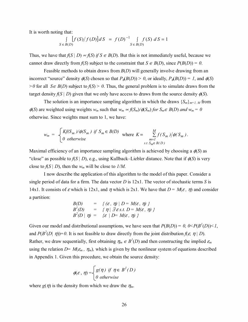
It is worth noting that: [ ]∫ =

∈ )()()(

DBSSdDfSf 1)()(

)(

1 ∫ =∈

−

DBSSdSfDf

Thus, we have that f(S | D) ∝ f(S) if S ∈ B(D). But this is not immediately useful, because we cannot draw directly from f(S) subject to the constraint that S ∈ B(D), since P(B(D)) = 0.

Feasible methods to obtain draws from B(D) will generally involve drawing from an incorrect “source” density φ(S) chosen so that Pφ(B(D)) > 0, or ideally, Pφ(B(D)) = 1, and φ(S) >0 for all S∈ B(D) subject to f(S) > 0. Thus, the general problem is to simulate draws from the target density f(S | D) given that we only have access to draws from the source density φ(S).

The solution is an importance sampling algorithm in which the draws {Sm}m=1, M from φ(S) are weighted using weights wm such that wm ∝ f(Sm)/φ(Sm) for Sm∈ B(D) and wm = 0 otherwise. Since weights must sum to 1, we have:

wm = otherwise 0

B(D) Sif )(S)/Kf(S mmm ∈φ where ∑=

∈=

M

)D(BS.t.s1m

mm

m

)S()S(fK φ .

Maximal efficiency of an importance sampling algorithm is achieved by choosing a φ(S) as “close” as possible to f(S | D), e.g., using Kullback–Liebler distance. Note that if φ(S) is very close to f(S | D), then the wm will be close to 1/M.

I now describe the application of this algorithm to the model of this paper. Consider a single period of data for a firm. The data vector D is 12x1. The vector of stochastic terms S is 14x1. It consists of ε which is 12x1, and η which is 2x1. We have that D = M(ε , η) and consider a partition:

B(D) = { (ε , η) | D = M(ε , η) } B1(D) = { η | ∃ ε s.t. D = M(ε , η) } B2(D | η) = {ε | D= M(ε , η) }

Given our model and distributional assumptions, we have seen that P(B(D)) = 0, 0<P(B1(D))<1, and P(B2(D| η))=0. It is not feasible to draw directly from the joint distribution f(ε, η | D). Rather, we draw sequentially, first obtaining ηm ∈ B1(D) and then constructing the implied εm using the relation D= M(εm , ηm), which is given by the nonlinear system of equations described in Appendix 1. Given this procedure, we obtain the source density:

φ(ε , η) = otherwise0

)D(Bif)g( 1∈ηη

where g(η) is the density from which we draw the ηm.

27

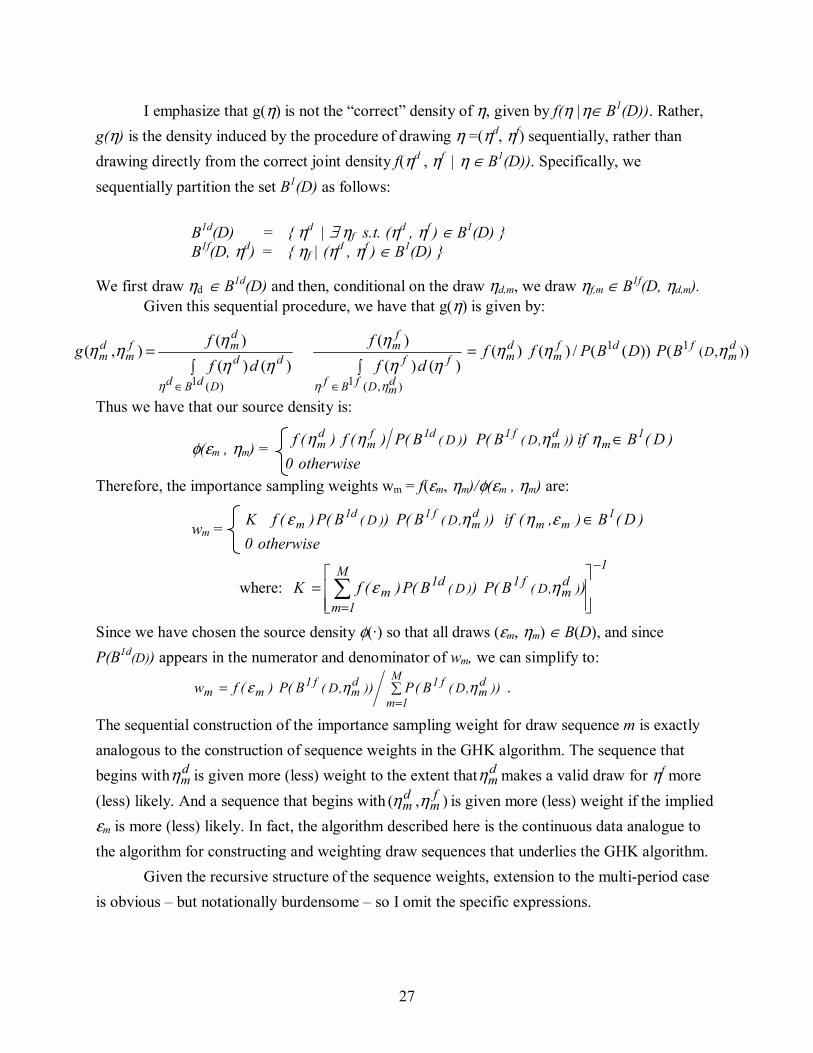
I emphasize that g(η) is not the “correct” density of η, given by f(η |η∈ B1(D)). Rather, g(η) is the density induced by the procedure of drawing η =(ηd, ηf) sequentially, rather than drawing directly from the correct joint density f(ηd , ηf | η ∈ B1(D)). Specifically, we sequentially partition the set B1(D) as follows:

B1d(D) = { ηd | ∃ ηf s.t. (ηd , ηf ) ∈ B1(D) } B1f(D, ηd) = { ηf | (ηd , ηf ) ∈ B1(D) }

We first draw ηd ∈ B1d(D) and then, conditional on the draw ηd,m, we draw ηf,m ∈ B1f(D, ηd,m).

Given this sequential procedure, we have that g(η) is given by:

)())((/)()()()(

)()()(

)(),( ),(11

),(1)(1

dm

fdfm

dm

dmDfBf

ff

fm

DdBd

dd

dmf

mdm DBPDBPff

dff

dff

g ηηηηη

ηηη

ηηη

ηηη

=∫∫

=

∈∈

Thus we have that our source density is:

φ(εm , ηm) = otherwise0

)D(Bif)B(P)B(P)(f)(f 1m

dm

f1d1fm

dm ),D()D( ∈ηηηη

Therefore, the importance sampling weights wm = f(εm, ηm)/φ(εm , ηm) are:

wm = otherwise0

)D(B),(if)B(P)B(P)(fK 1mm

dm

f1d1m ),D()D( ∈εηηε

where: 1M

1m)d

m,D(f1)D(d1m )B(P)B(P)(fK

−

=

= ∑ ηε

Since we have chosen the source density φ(·) so that all draws (εm, ηm) ∈ B(D), and since P(B1d(D)) appears in the numerator and denominator of wm, we can simplify to:

∑==

M

1m

dm

f1dm

f1mm )B(P)B(P)(fw ),D(),D( ηηε .

The sequential construction of the importance sampling weight for draw sequence m is exactly analogous to the construction of sequence weights in the GHK algorithm. The sequence that begins with d

mη is given more (less) weight to the extent that dmη makes a valid draw for ηf more

(less) likely. And a sequence that begins with ),( fm

dm ηη is given more (less) weight if the implied

εm is more (less) likely. In fact, the algorithm described here is the continuous data analogue to the algorithm for constructing and weighting draw sequences that underlies the GHK algorithm. Given the recursive structure of the sequence weights, extension to the multi-period case is obvious – but notationally burdensome – so I omit the specific expressions.

28

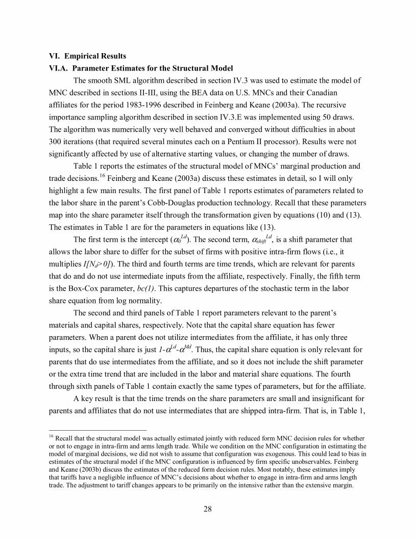
VI. Empirical Results VI.A. Parameter Estimates for the Structural Model

The smooth SML algorithm described in section IV.3 was used to estimate the model of MNC described in sections II-III, using the BEA data on U.S. MNCs and their Canadian affiliates for the period 1983-1996 described in Feinberg and Keane (2003a). The recursive importance sampling algorithm described in section IV.3.E was implemented using 50 draws. The algorithm was numerically very well behaved and converged without difficulties in about 300 iterations (that required several minutes each on a Pentium II processor). Results were not significantly affected by use of alternative starting values, or changing the number of draws.

Table 1 reports the estimates of the structural model of MNCs’ marginal production and trade decisions.16 Feinberg and Keane (2003a) discuss these estimates in detail, so I will only highlight a few main results. The first panel of Table 1 reports estimates of parameters related to the labor share in the parent’s Cobb-Douglas production technology. Recall that these parameters map into the share parameter itself through the transformation given by equations (10) and (13). The estimates in Table 1 are for the parameters in equations like (13).

The first term is the intercept (α0Ld). The second term, αshift

Ld, is a shift parameter that allows the labor share to differ for the subset of firms with positive intra-firm flows (i.e., it multiplies I[Nd>0]). The third and fourth terms are time trends, which are relevant for parents that do and do not use intermediate inputs from the affiliate, respectively. Finally, the fifth term is the Box-Cox parameter, bc(1). This captures departures of the stochastic term in the labor share equation from log normality.

The second and third panels of Table 1 report parameters relevant to the parent’s materials and capital shares, respectively. Note that the capital share equation has fewer parameters. When a parent does not utilize intermediates from the affiliate, it has only three inputs, so the capital share is just 1-αLd-αMd. Thus, the capital share equation is only relevant for parents that do use intermediates from the affiliate, and so it does not include the shift parameter or the extra time trend that are included in the labor and material share equations. The fourth through sixth panels of Table 1 contain exactly the same types of parameters, but for the affiliate.

A key result is that the time trends on the share parameters are small and insignificant for parents and affiliates that do not use intermediates that are shipped intra-firm. That is, in Table 1,

16 Recall that the structural model was actually estimated jointly with reduced form MNC decision rules for whether or not to engage in intra-firm and arms length trade. While we condition on the MNC configuration in estimating the model of marginal decisions, we did not wish to assume that configuration was exogenous. This could lead to bias in estimates of the structural model if the MNC configuration is influenced by firm specific unobservables. Feinberg and Keane (2003b) discuss the estimates of the reduced form decision rules. Most notably, these estimates imply that tariffs have a negligible influence of MNC’s decisions about whether to engage in intra-firm and arms length trade. The adjustment to tariff changes appears to be primarily on the intensive rather than the extensive margin.

29

the terms αTimeLd⋅t ⋅ I[Nd=0], αTime

Md⋅t ⋅ I[Nd=0], αTimeL f⋅t ⋅ I[Nf=0] and αTime

Mf⋅t ⋅ I[Nf=0] are all insignificant and quantitatively small. Thus, the behavior of these parents and affiliates is well described by a CRTS Cobb-Douglas technology with fixed share parameters.

In contrast, for the subset of MNC parents that do utilize intermediates from affiliates, and affiliates that use intermediates from parents, the time trends for the share parameters are all highly significant and negative. Recall that these trends feed into logistic transformations like (10). Thus, the fact that the time trends are negative for labor, capital and materials means the share of the omitted category (intermediates) must be rising. Thus, conditional on MNCs having had positive intra-firm flows initially, the estimates imply that “technical change” was driving up the share of intermediates.

Another way to state this result is that the model cannot explain the observed increase in intra-firm trade in intermediates based on the changes in the exogenous forcing variables, such as tariffs, transport costs, exchange rates, wages, materials prices, etc.. Thus, the model attributes the increase in intra-firm trade to technological change in the form of trends in the Cobb-Douglas share parameters. Feinberg and Keane (2003a) discuss this result at length and argue that it would be robust to various changes in the structural model that has been estimated here. They also argue that these “technical change” estimates may be picking up recent advances in logistics that have made it easier to ship intermediates intra-firm in a way that allows fragmented production processes to operate smoothly.

The top four panels on the second page of Table 1 contain estimates of the labor cost adjustment cost function. In the top two panels note that time trends in the δd and δf equations (see equation 18) are both significant and positive, suggesting that labor force adjustment costs increased over time. The third panel contains estimates of the µ and ∆ parameters in the generalized labor force adjustment cost function (equation 5). These estimates imply that adjustment costs are not well described by the common linear-quadratic in levels specification, since they depart substantially from µ=1 and ∆=0. The fact that µ<1 and ∆>0 implies that the cost of a given absolute change in labor force size is smaller to the extent that the change represents a smaller fraction of the initial labor force.

The fourth panel contains estimates of the parameters τ that determine the variance of labor adjustment forecast errors (see equation 22). Not surprisingly, forecast error variance is increasing in labor force size. Interestingly, the domestic forecast error variance is higher (for given labor force size), and domestic and foreign forecast errors are positively correlated.

The middle two panels on the second page of Table 1 contain estimates of the parameters that determine the (negative) inverse price elasticities of demand for the U.S. and Canadian produced good (g1 and g2). These are the parameters of equations like (16). Note that the Box-Cox parameter for g1, which is .6084, implies that a transform close to the square root is needed

30

to induce normality of the residuals, while the transform for g2, which is .8424, is quite close to linear. Thus, the stochastic terms in the g equations depart dramatically from log normality.

The last four panels on page 2 of Table 1 contain estimates of the parameters that determine the four demand function intercept parameters (i.e. U.S. and Canadian demand for the U.S. and Canadian produced goods). These are the parameters of equations like (17). Note that all four demand function intercepts exhibit significant negative time trends, implying falling demand at any given price level. At the same time, the estimate of TFP growth is 4.5% per year. As I discuss in Appendix 2, as g→1 (less elastic demand) TFP growth has no effect on employment. Thus, the fact that TFP is increasing while demand (at any given price) is falling implies that growth in employment is very concentrated among firms facing elastic demand. In fact, employment must be shrinking among high market power firms (see the discussion of Table 5 in section VI.C for more on this point).

Finally, I turn the estimates of the covariance matrix of the firm specific stochastic terms. Each of the 12 technology and demand function parameters is allowed to be heterogeneous across firms and over time. Recall from Section III.4 that I specify a stochastic structure where each of these 12 parameters has a firm/time specific component that consists of a random effect, µi, and a transitory error, νit. Table 2 reports estimates of the correlation matrices of these stochastic terms. Panel 1 presents the cross-sectional correlation matrix of the composite error µi+νit. Although all correlations are highly significant, the smallest (about 0.4) are for the country specific demand shifters across the two different goods (i.e., between 1

d0P and 2d0P , and

between 1d0P and 2

f0P ). By contrast, the correlation between the U.S. and Canadian demand shifters for the domestically produced good (i.e., between 1

d0P and 1f0P ) is 0.97! That is, demand

for the same good across the two countries is extremely highly correlated, while demand for the two different goods in the same country is not so highly correlated.

The second panel of Table 2 reports the correlations of the firm specific parameters at times t and t+1. The random effects structure implies equal correlations at all leads and lags, all the way out to t+11. As we would expect, all the firm specific parameters are highly serially correlated. The technology and demand function intercept parameters show more persistence (i.e., correlations in the 0.72 to 0.80 range) than do the market power parameters (i.e., correlations of 0.46 and 0.53).

VI.B. Fit of the Structural Model

The SML based on FOCs estimation method requires that the researcher specify a joint parametric distribution for the vector of stochastic terms in the model. Thus, it is important to have a method to test the validity of the assumed parametric distribution. In the illustrative model of MNC behavior that I have estimated in this paper, I assumed that the vector of 12 firm

31

specific technology and demand parameters are jointly normally distributed, subject to a Box-Cox transformation (as described in section III). In order to investigate the validity of this assumption, I use the recursive importance sampling algorithm developed in Section V to draw from the posterior distribution of the stochastic terms for each firm, conditional on the estimated model and the firm’s observed history. I then use these draws to test the joint normality assumption.

Specifically, I use the algorithm developed in Section V to draw ten vectors of simulated residuals (and their associated importance sampling weights) for each observation in the data set. Tables 3 and 4 report two tests of the normality assumption based on these simulated residuals.

Table 3 presents χ2 tests of normality based on the deciles of the normal distribution. These tests show that the normality assumption is substantially supported. Indeed, I reject normality at the 1% level for only one of the 12 residuals—the affiliate materials share—and at the 5% level, I reject normality only for one additional residual—the parent capital share.17 Table 4 presents the simulated deciles for each residual, and compares these to the deciles of the standard normal distribution. Starred entries in Table 4 denote deciles of the residuals that depart significantly from normality. Only the deciles for the parent capital and affiliate materials shares show any significant departures from the deciles of the normal distribution. I can reject normality for four of the deciles of the αKd residual and two of the deciles of the αMf residual. However, even in these worst cases, the departures from normality are not dramatic.

Recall that a novel feature of SML based on FOCs approach when applied to dynamic models is the assumption that forecast errors are normal. This is also a feature of the pseudo-SML based on FOCs approach developed in Krusell, Ohanian, Rios-Rull and Violante (2000). Traditionally, researchers have been reluctant to specify that forecast errors have any particular parametric distribution, such as normality, because there is no theoretical reason to expect them to have any particular distribution. Thus, it is important that we have a means of testing the normality assumption.

The statistics in Table 4 indicate strong support for the normality assumption on the forecast errors. According to the results in Table 4 the deciles of the simulated distributions for the domestic and foreign labor force adjustment cost forecast errors, ηd and ηf are essentially indistinguishable from normality. This finding is particularly encouraging with regard to the potential usefulness of the SML based on FOCs approach.

In summary, the model appears to fit the data quite well, in the sense that the parametric assumptions on the distributions of the stochastic terms appear (for the most part) to be strongly supported. 17 The test statistic is χ2 (9), based upon the deciles of the normal distribution. I bootstrap the critical values to deal with the fact that residuals for a firm are highly serially correlated.

32

VI.C. Some Simulation Experiments A key advantage of the SML based on FOCs approach over GMM is that, in conjunction with the sampling algorithm developed in section V, it enables one to draw from the posterior distribution of the firm specific parameters (conditional on the model and the data). Given such draws, we can simulate the behavior of individual firms, and/or the whole population of firms, to changes in the economic environment. The GMM approach does not allow this, because it does not deliver estimates of the distributions of the stochastic terms.

On the other hand, in the SML based on FOCs approach the model is not completely specified. In the present case, I have not specified the stochastic processes for the forcing processes such as tariffs, exchange rates, wages, technical change, etc., nor have I specified how firms form expectations of future values of these quantities. Since I have not implemented a full-solution algorithm, I cannot simulate the short-run outcomes generated by the dynamic model. To do the latter would require a complete model, which could be estimated using FIML. However, I can use a steady-state version of the model (which assumes no labor force adjustment costs) to simulate the long-run response of the population of firms to changes in the policy environment.

In Table 5, I use simulations of the model to examine the effect of various changes in the economic environment on MNC behavior. The simulations are done using 543 vectors of technology and demand parameters drawn from the posterior distribution of the firm specific parameters of the model, using eth algorithm of Section V. Feinberg and Keane (2003a) discuss these simulations in detail, so here I just give some highlights.

The first column of Table 5 reports the actual changes in several variables of interest that occurred from 1984-1995. The second column reports the predicted change from 1984 to 1995 in the steady state level of each variable, given all changes in the environment. The third, fourth and fifth columns report the predicted changes due to changes in tariffs, technology and wages, respectively. The last column reports the combined effect of all other factors in the model.

Of course, the predicted change in steady state levels is not directly comparable to the change in actuals, since the latter include transition dynamics. However, from a face validity standpoint it is comforting that the predicted changes line up reasonably well with the actual changes. For example, the model predicts that all factors combined led to an increase of 99% in U.S. parent intra-firm sales to affiliates, and a 79% increase in U.S. parent arms-length sales to Canada. The actual changes were 73% and 75% respectively. And the model predicts that all factors combined lead to a 123% increase in affiliate intra-firm sales to parents, and a 9% increase in affiliates arms-length sales to the U.S.. The actual changes were 95% and 4% respectively. It is interesting that employment falls both in the data and according to the model. As I discussed in Section VI.A, this is consistent with the pattern we would expect for firms with

33

substantial market power, given that TFP increased while demand (and any given price) fell over the sample period.

Now lets look at the model’s decomposition of how specific exogenous factors affected MNC behavior over the sample period. The model predicts that tariff reductions over the 1984-1995 period increased U.S. parents’ arms length sales to Canada by 36% and affiliates’ arms-length sales to the U.S. by 32.5%. Note, however, that affiliate arms-length sales to the U.S. only increase 4% in the data, and they only increased 9% in the simulation that takes all factors into account. According to the model, other factors were hindering Canadian affiliate arms-length exports to the U.S.. One key factor was rising Canadian real wages. The real wage (in U.S. dollar terms) paid by Canadian affiliates increased by 20% from 1984-1995. The model predicts that this reduced affiliates’ arms-length exports to the U.S. by 20%. Table 5 also reveals the important role that the model assigns to technical change in increasing intra-firm trade. Of the 99% increase in parents’ intra-firm sales to affiliates, the model attributes 72 percentage points to technical change. And of the 123% increase in affiliates’ intra-firm sales to parents, the model attributes 84 percentage points to technical change. The changes attributed to tariff reductions are only about 10 and 5 percentage points, respectively. While these tariff effects are not trivial, they are an order of magnitude smaller than the impact of technology. Feinberg and Keane (2003a) discuss possible technological reasons for the increase in intra-firm trade. VII. Conclusions In this paper I have described the SML based on FOCs approach for structural estimation of economic models. The approach is a compromise between GMM and FIML because the economic model does not have to be completely specified and fully solved, a feature the method shares with GMM. But parametric distributions must be specified for all the stochastic terms that appear in the FOCS, a feature the method has in common with FIML.

The key virtue of the method relative to GMM is that it allows for multiple sources of structural error, and hence enables one to model rich patterns of heterogeneity across economic agents. In contrast, to apply GMM to models with multiple sources of structural error, one typically needs strong functional form assumptions so that the FOCS can nevertheless be written in terms of a single additive composite error term.

There are two computational problems that will typically arise in applying the SML based on FOCs method. First, in a model where the stochastic terms enter the FOCs nonlinearly, it will typically be the case that the Jacobian of the transformation from the stochastic terms to the data will be intractable. I have shown how one can deal with this problem by using numerical and simulation methods to approximate the Jacobian.

34

Second, economic models often have the feature that for certain ranges of the stochastic terms the FOCs cannot be satisfied (i.e., we are at a corner solution where the firm shuts down, demand is zero, etc.). I have shown how to deal with this problem by developing a new recursive importance algorithm to simulate the likelihood function. This algorithm is based on drawing the stochastic terms from the “wrong” density, chosen in such a way that all draws from the density allow the FOCs to be satisfied. The importance sampling weights adjust for the fact that the “wrong” density is used. This algorithm is the discrete/continuous analogue of the GHK algorithm.

Once one has estimated a model using the SML based on FOCs method, it is desirable to be able to draw from the posterior distribution of the firm specific parameters. This is useful both because one would like to test ones distributional assumptions, and because one would like to be able to simulate the behavior of the economic agents in the model. The GMM approach does not allow this because it does not produce estimates of the distributions of a model’s stochastic terms. The SML based on FOCs approach does provide estimates of the distributions of the stochastic terms, so posterior simulation is in principle possible. However, such posterior simulation is in general a difficult problem in models where there is not a one-to-one mapping from the data to the stochastic terms. In models with rich patterns of heterogeneity across agents, there will typically be more stochastic terms than there are observed data elements.

To deal with this problem, I have presented a recursive importance algorithm that can be used to simulate from a J dimensional vector of agent specific stochastic terms that lie in a K dimensional sub-space, where K<J is determined by the constraints implied by the data and the FOCs. The particular problem one faces here is that the sub-space of valid draws has measure zero. The algorithm that I develop to draw from such a sub-space is the continuous data analogue of the GHK algorithm.

The methods developed in the paper were applied to an illustrative model of the behavior of U.S. MNCs with affiliates in Canada. The methods appeared to work well in practice, and the estimates were numerically well behaved. Interestingly, there appeared to be little evidence against the distributional assumptions of the model, particularly the assumption of normally distributed forecast errors. This seems encouraging from the perspective of future application of the method.

35

References Ackerberg, D. and K. Caves (2003), “Structural Estimation of Production Functions,” Working

paper, UCLA. Eden, L. 1998. Taxing Multinationals: Transfer Pricing and Corporate Income Taxation in

North America. Toronto: University of Toronto Press. Feinberg, S. E. and M.P. Keane (2003a), “Accounting for the Growth of MNC Based Trade

Using a Structural Model of U.S. MNCs,” Working paper, University of Maryland. Feinberg, S. E. and M.P. Keane (2003b), “Tariff effects on MNC organization,” Working paper,

University of Maryland. Griliches, Z. and J. Mairesse, (1995), “Production Functions: The Search for Identification,”

NBER Working Paper #5067. Hansen, L. P. (1982), “Large Sample Properties of Generalized Method of Moments

Estimators,” Econometrica, Vol. 50, No. 4., pp. 1029-1054.

Hansen, L. P. and K. J. Singleton (1982), “Generalized Instrumental Variables Estimation of Nonlinear Rational Expectations Models,” Econometrica, Vol. 50, No. 5., pp. 1269-1286.

Katayama, H., Lu, S. and J. Tybout, (2003), “Why Plant-Level Productivity Studies are Often

Misleading, and an Alternative Approach to Interference,” NBER Working Paper #9617. Keane, M. (1994), “A Computationally Practical Simulation Estimator for Panel Data,”

Econometrica, Vol. 62, No. 1. (Jan., 1994), pp. 95-116. Klette, T.J. and Z. Griliches, 1996. The Inconsistency of Common Scale Estimators When

Output Prices Are Unobserved and Endogenous, NBER Working Paper# 4026. Krusell, P., Ohanian, L. E., Ríos-Rull, J.V., and G. L. Violante (2000), “Capital-Skill

Complementarity and Inequality: A Macroeconomic Analysis,” Econometrica, 68:5, p.1029. Lee, L. F. (1992), “On the Efficiency of Methods of Simulated Moments and Maximum

Simulated Likelihood Estimation of Discrete Response Models,” Econometric Theory, 8, pp. 518-552.

Lee, L. F. (1995), “Asymptotic Bias in Maximum Simulated Likelihood Estimation of Discrete

Choice Models,” Econometric Theory, 11, pp. 437-483. Levinsohn, J. and M. Melitz (2002), “Productivity in a Differentiated Products Market

Equilibrium,” Working paper, University of Michigan. McCallum, B.T. (1976), “Rational Expectations and the Natural Rate Hypothesis: Some Consistent Estimates,” Econometrica, Vol. 44, No. 1., pp. 43-52.

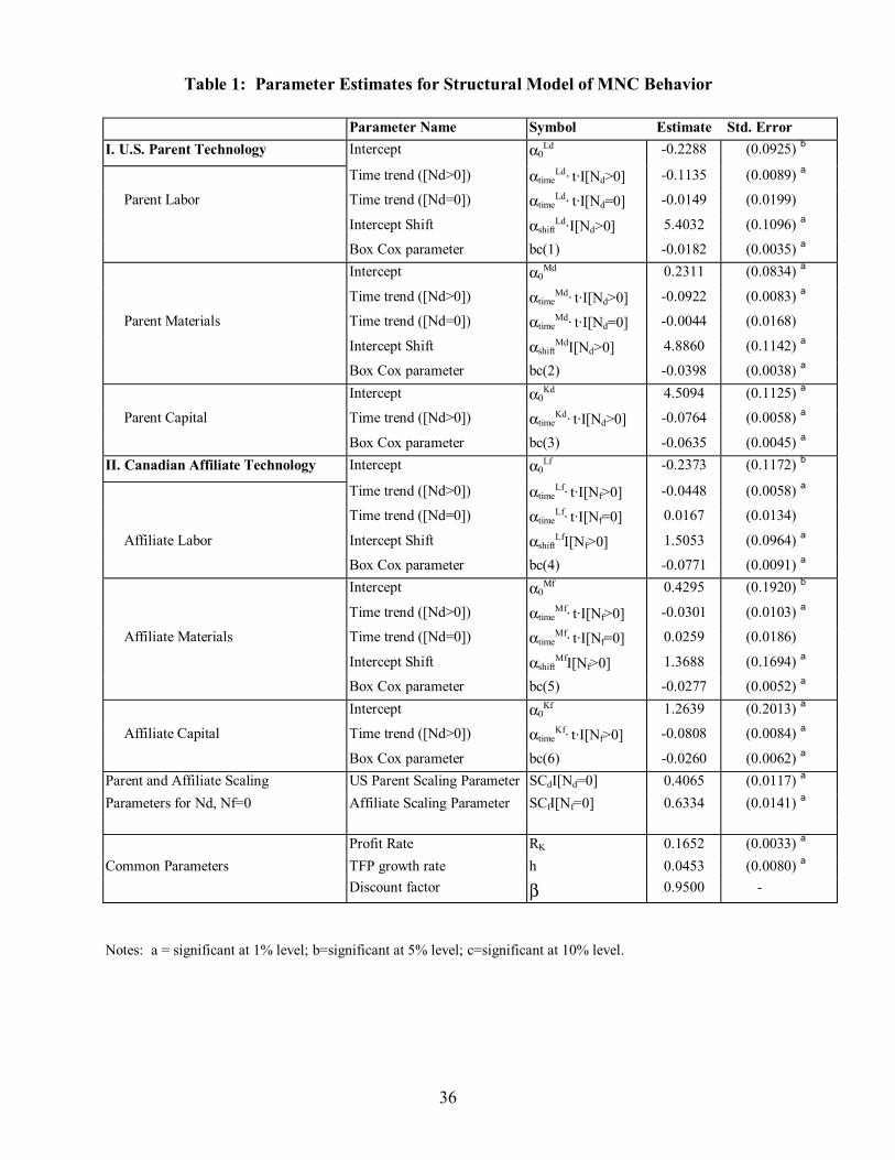
36

Table 1: Parameter Estimates for Structural Model of MNC Behavior Parameter Name Symbol Estimate Std. Error

I. U.S. Parent Technology Intercept α0Ld -0.2288 (0.0925) b

Time trend ([Nd>0]) αtimeLd· t·I[Nd>0] -0.1135 (0.0089) a

Parent Labor Time trend ([Nd=0]) αtimeLd· t·I[Nd=0] -0.0149 (0.0199)

Intercept Shift αshiftLd·I[Nd>0] 5.4032 (0.1096) a

Box Cox parameter bc(1) -0.0182 (0.0035) a

Intercept α0Μd 0.2311 (0.0834) a

Time trend ([Nd>0]) αtimeMd· t·I[Nd>0] -0.0922 (0.0083) a

Parent Materials Time trend ([Nd=0]) αtimeMd· t·I[Nd=0] -0.0044 (0.0168)

Intercept Shift αshiftMdI[Nd>0] 4.8860 (0.1142) a

Box Cox parameter bc(2) -0.0398 (0.0038) a

Intercept α0Kd 4.5094 (0.1125) a

Parent Capital Time trend ([Nd>0]) αtimeKd· t·I[Nd>0] -0.0764 (0.0058) a

Box Cox parameter bc(3) -0.0635 (0.0045) a

II. Canadian Affiliate Technology Intercept α0Lf -0.2373 (0.1172) b

Time trend ([Nd>0]) αtimeLf· t·I[Nf>0] -0.0448 (0.0058) a

Time trend ([Nd=0]) αtimeLf· t·I[Nf=0] 0.0167 (0.0134)

Affiliate Labor Intercept Shift αshiftLfI[Nf>0] 1.5053 (0.0964) a

Box Cox parameter bc(4) -0.0771 (0.0091) a

Intercept α0Μf 0.4295 (0.1920) b

Time trend ([Nd>0]) αtimeMf· t·I[Nf>0] -0.0301 (0.0103) a

Affiliate Materials Time trend ([Nd=0]) αtimeMf· t·I[Nf=0] 0.0259 (0.0186)

Intercept Shift αshiftMfI[Nf>0] 1.3688 (0.1694) a

Box Cox parameter bc(5) -0.0277 (0.0052) a

Intercept α0Kf 1.2639 (0.2013) a

Affiliate Capital Time trend ([Nd>0]) αtimeKf· t·I[Nf>0] -0.0808 (0.0084) a

Box Cox parameter bc(6) -0.0260 (0.0062) a

Parent and Affiliate Scaling US Parent Scaling Parameter SCdI[Nd=0] 0.4065 (0.0117) a

Parameters for Nd, Nf=0 Affiliate Scaling Parameter SCfI[Nf=0] 0.6334 (0.0141) a

Profit Rate RK 0.1652 (0.0033) a

Common Parameters TFP growth rate h 0.0453 (0.0080) a

Discount factor β 0.9500 -

Notes: a = significant at 1% level; b=significant at 5% level; c=significant at 10% level.

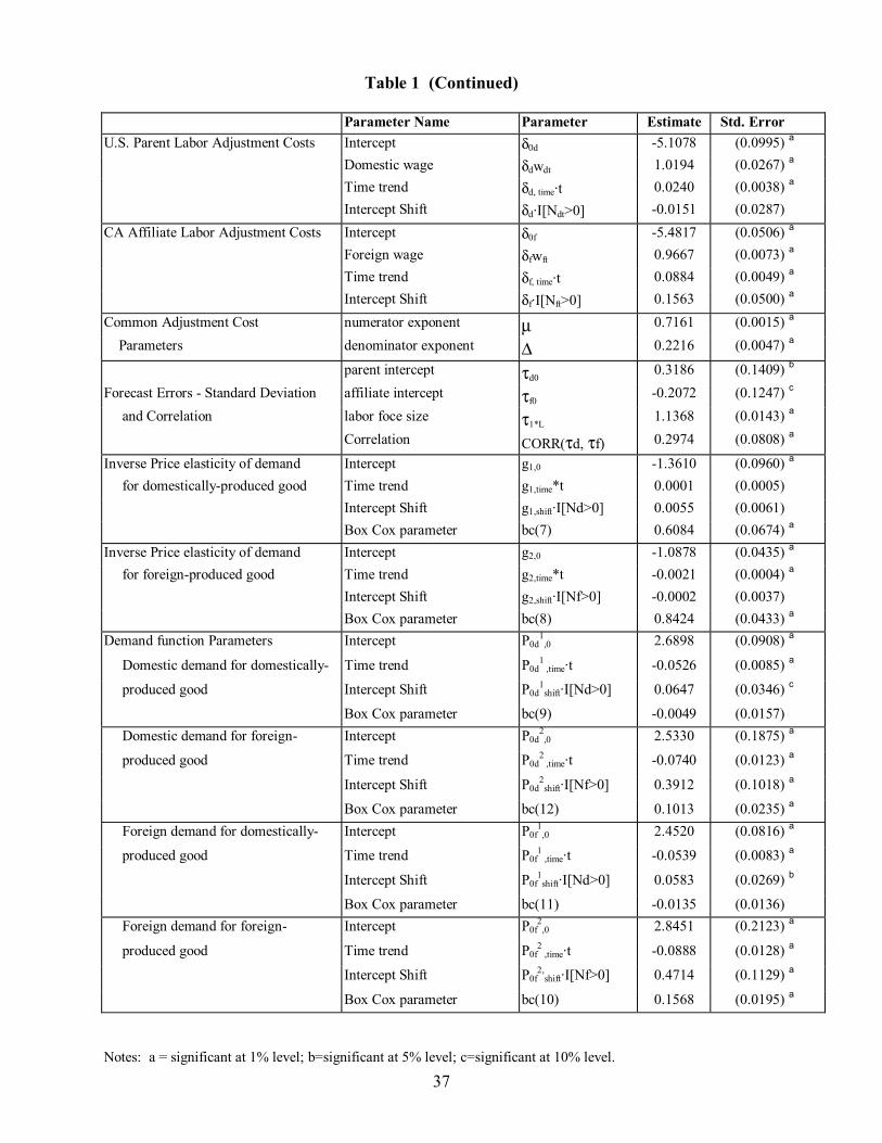
37

Table 1 (Continued)

Parameter Name Parameter Estimate Std. Error

U.S. Parent Labor Adjustment Costs Intercept δ0d -5.1078 (0.0995) a

Domestic wage δdwdt 1.0194 (0.0267) a

Time trend δd, time·t 0.0240 (0.0038) a

Intercept Shift δd·I[Ndt>0] -0.0151 (0.0287)

CA Affiliate Labor Adjustment Costs Intercept δ0f -5.4817 (0.0506) a

Foreign wage δfwft 0.9667 (0.0073) a

Time trend δf, time·t 0.0884 (0.0049) a

Intercept Shift δf·I[Nft>0] 0.1563 (0.0500) a

Common Adjustment Cost numerator exponent µ 0.7161 (0.0015) a

Parameters denominator exponent ∆ 0.2216 (0.0047) a

parent intercept τd0 0.3186 (0.1409) b

Forecast Errors - Standard Deviation affiliate intercept τf0 -0.2072 (0.1247) c

and Correlation labor foce size τ1*L 1.1368 (0.0143) a

Correlation CORR(τd, τf) 0.2974 (0.0808) a

Inverse Price elasticity of demand Intercept g1,0 -1.3610 (0.0960) a

for domestically-produced good Time trend g1,time*t 0.0001 (0.0005)

Intercept Shift g1,shift·I[Nd>0] 0.0055 (0.0061)

Box Cox parameter bc(7) 0.6084 (0.0674) a

Inverse Price elasticity of demand Intercept g2,0 -1.0878 (0.0435) a

for foreign-produced good Time trend g2,time*t -0.0021 (0.0004) a

Intercept Shift g2,shift·I[Nf>0] -0.0002 (0.0037)

Box Cox parameter bc(8) 0.8424 (0.0433) a

Demand function Parameters Intercept P0d1

,0 2.6898 (0.0908) a

Domestic demand for domestically- Time trend P0d1

,time·t -0.0526 (0.0085) a

produced good Intercept Shift P0d1

shift·I[Nd>0] 0.0647 (0.0346) c

Box Cox parameter bc(9) -0.0049 (0.0157)

Domestic demand for foreign- Intercept P0d2

,0 2.5330 (0.1875) a

produced good Time trend P0d2

,time·t -0.0740 (0.0123) a

Intercept Shift P0d2

shift·I[Nf>0] 0.3912 (0.1018) a

Box Cox parameter bc(12) 0.1013 (0.0235) a

Foreign demand for domestically- Intercept P0f1

,0 2.4520 (0.0816) a

produced good Time trend P0f1

,time·t -0.0539 (0.0083) a

Intercept Shift P0f1

shift·I[Nd>0] 0.0583 (0.0269) b

Box Cox parameter bc(11) -0.0135 (0.0136)

Foreign demand for foreign- Intercept P0f2

,0 2.8451 (0.2123) a

produced good Time trend P0f2

,time·t -0.0888 (0.0128) a

Intercept Shift P0f2,

shift·I[Nf>0] 0.4714 (0.1129) a

Box Cox parameter bc(10) 0.1568 (0.0195) a

Notes: a = significant at 1% level; b=significant at 5% level; c=significant at 10% level.

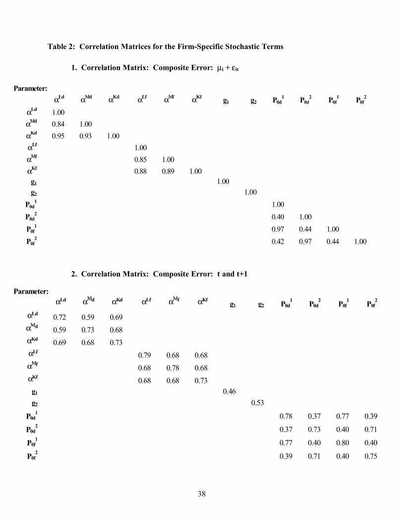
38

Table 2: Correlation Matrices for the Firm-Specific Stochastic Terms

1. Correlation Matrix: Composite Error: µi + εit

2. Correlation Matrix: Composite Error: t and t+1

Parameter:αLd αΜd αKd αLf αΜf αKf g1 g2 P0d

1 P0d2 P0f

1 P0f2

αLd 0.72 0.59 0.69αΜd 0.59 0.73 0.68αKd 0.69 0.68 0.73αLf 0.79 0.68 0.68αΜf 0.68 0.78 0.68αKf 0.68 0.68 0.73g1 0.46g2 0.53

P0d1 0.78 0.37 0.77 0.39

P0d2 0.37 0.73 0.40 0.71

P0f1 0.77 0.40 0.80 0.40

P0f2 0.39 0.71 0.40 0.75

Parameter:αLd αΜd αKd αLf αΜf αKf g1 g2 P0d

1 P0d2 P0f

1 P0f2

αLd 1.00αΜd 0.84 1.00αKd 0.95 0.93 1.00αLf 1.00αΜf 0.85 1.00αKf 0.88 0.89 1.00g1 1.00g2 1.00

P0d1 1.00

P0d2 0.40 1.00

P0f1 0.97 0.44 1.00

P0f2 0.42 0.97 0.44 1.00

39

Table 3: χ2 Tests of Normality based on Deciles of the Normal (0,1) Distribution Residual χ2 Residual χ2 Residual χ2

αLd 9.549 g1 8.583 τd0 9.138 αMd 8.559 g2 11.195 τf0 0.512 αKd 18.454* P0d

1 4.257 αLf 2.983 P0d

2 2.759 αMf 27.958* P0f

1 5.131 αKf 11.889 P0f

2 7.978

*Rejected at p<.05, based on the bootstrapped critical value of the χ2 distribution

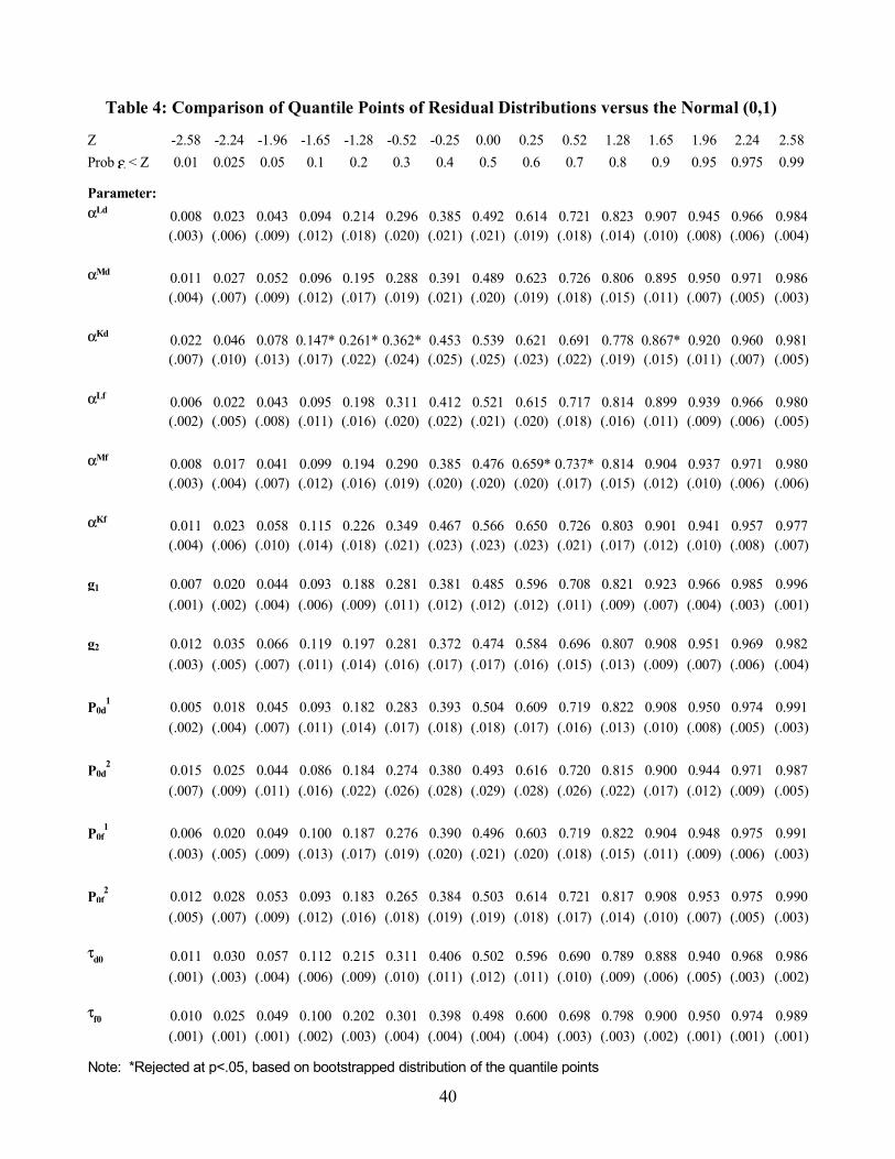
40

Table 4: Comparison of Quantile Points of Residual Distributions versus the Normal (0,1)

Z -2.58 -2.24 -1.96 -1.65 -1.28 -0.52 -0.25 0.00 0.25 0.52 1.28 1.65 1.96 2.24 2.58Prob ε < Z 0.01 0.025 0.05 0.1 0.2 0.3 0.4 0.5 0.6 0.7 0.8 0.9 0.95 0.975 0.99

Parameter:αLd 0.008 0.023 0.043 0.094 0.214 0.296 0.385 0.492 0.614 0.721 0.823 0.907 0.945 0.966 0.984

(.003) (.006) (.009) (.012) (.018) (.020) (.021) (.021) (.019) (.018) (.014) (.010) (.008) (.006) (.004)

αMd 0.011 0.027 0.052 0.096 0.195 0.288 0.391 0.489 0.623 0.726 0.806 0.895 0.950 0.971 0.986(.004) (.007) (.009) (.012) (.017) (.019) (.021) (.020) (.019) (.018) (.015) (.011) (.007) (.005) (.003)

αKd 0.022 0.046 0.078 0.147* 0.261* 0.362* 0.453 0.539 0.621 0.691 0.778 0.867* 0.920 0.960 0.981(.007) (.010) (.013) (.017) (.022) (.024) (.025) (.025) (.023) (.022) (.019) (.015) (.011) (.007) (.005)

αLf 0.006 0.022 0.043 0.095 0.198 0.311 0.412 0.521 0.615 0.717 0.814 0.899 0.939 0.966 0.980(.002) (.005) (.008) (.011) (.016) (.020) (.022) (.021) (.020) (.018) (.016) (.011) (.009) (.006) (.005)

αMf 0.008 0.017 0.041 0.099 0.194 0.290 0.385 0.476 0.659* 0.737* 0.814 0.904 0.937 0.971 0.980(.003) (.004) (.007) (.012) (.016) (.019) (.020) (.020) (.020) (.017) (.015) (.012) (.010) (.006) (.006)

αKf 0.011 0.023 0.058 0.115 0.226 0.349 0.467 0.566 0.650 0.726 0.803 0.901 0.941 0.957 0.977(.004) (.006) (.010) (.014) (.018) (.021) (.023) (.023) (.023) (.021) (.017) (.012) (.010) (.008) (.007)

g1 0.007 0.020 0.044 0.093 0.188 0.281 0.381 0.485 0.596 0.708 0.821 0.923 0.966 0.985 0.996(.001) (.002) (.004) (.006) (.009) (.011) (.012) (.012) (.012) (.011) (.009) (.007) (.004) (.003) (.001)

g2 0.012 0.035 0.066 0.119 0.197 0.281 0.372 0.474 0.584 0.696 0.807 0.908 0.951 0.969 0.982(.003) (.005) (.007) (.011) (.014) (.016) (.017) (.017) (.016) (.015) (.013) (.009) (.007) (.006) (.004)

P0d1 0.005 0.018 0.045 0.093 0.182 0.283 0.393 0.504 0.609 0.719 0.822 0.908 0.950 0.974 0.991

(.002) (.004) (.007) (.011) (.014) (.017) (.018) (.018) (.017) (.016) (.013) (.010) (.008) (.005) (.003)

P0d2 0.015 0.025 0.044 0.086 0.184 0.274 0.380 0.493 0.616 0.720 0.815 0.900 0.944 0.971 0.987

(.007) (.009) (.011) (.016) (.022) (.026) (.028) (.029) (.028) (.026) (.022) (.017) (.012) (.009) (.005)

P0f1 0.006 0.020 0.049 0.100 0.187 0.276 0.390 0.496 0.603 0.719 0.822 0.904 0.948 0.975 0.991

(.003) (.005) (.009) (.013) (.017) (.019) (.020) (.021) (.020) (.018) (.015) (.011) (.009) (.006) (.003)

P0f2 0.012 0.028 0.053 0.093 0.183 0.265 0.384 0.503 0.614 0.721 0.817 0.908 0.953 0.975 0.990

(.005) (.007) (.009) (.012) (.016) (.018) (.019) (.019) (.018) (.017) (.014) (.010) (.007) (.005) (.003)

τd0 0.011 0.030 0.057 0.112 0.215 0.311 0.406 0.502 0.596 0.690 0.789 0.888 0.940 0.968 0.986(.001) (.003) (.004) (.006) (.009) (.010) (.011) (.012) (.011) (.010) (.009) (.006) (.005) (.003) (.002)

τf0 0.010 0.025 0.049 0.100 0.202 0.301 0.398 0.498 0.600 0.698 0.798 0.900 0.950 0.974 0.989(.001) (.001) (.001) (.002) (.003) (.004) (.004) (.004) (.004) (.003) (.003) (.002) (.001) (.001) (.001)

Note: *Rejected at p<.05, based on bootstrapped distribution of the quantile points

41

Table 5: Percentage Changes 1984-1995: Data and Model Predictions

Model Decomposition Data Model Tariffs Technology Wages Other

USP Sales

Domestic (Pd1Sd) -19.6 -9.0 0.8 4.0 -4.3 -9.5

Intra-firm (Pd1Nf) 73.3 99.1 9.7 71.8 14.4 3.2

Arms-Length (Pf1E) 75.3 79.1 36.0 9.0 -1.3 35.4

Total -17.1 -6.0 1.1 7.3 -3.9 -10.5Total Net -20.2 -9.8 1.0 3.8 -3.9 -10.7

CA Sales

Domestic (Pf2Sf) -17.9 -6.9 6.4 -71.9 18.3 40.3

Intra-firm (Pf2Nd) 94.5 123 5.2 84.1 -2.9 36.6

Arms-Length (Pd2I) 4.0 8.9 32.5 37.9 -20.5 -41.0

Total 18.7 38.3 7.3 7.8 11.2 12.0Total Net -0.5 14.2 6.3 -23.3 9.9 21.3

MNC Sales -19.0 -8.4 1.3 2.4 -3.0 -9.1

USP Employment -24.4 -12.6 1.4 12.4 -1.6 -24.8CA Employment -14.1 -3.0 9.0 15.5 -7.0 -20.5 Notes: "Data" shows percentage change in our analysis data set. "Model" shows percentage change from 1984-95 in the model simulation. Under "Model Decomposition," we compare the % change predicted by the model under the baseline simulation, with the % change the model predicts under the counterfactual that the indicated forcing variable (tariffs, technology or wages) stayed fixed at the 1984 level. The difference is the percentage change attributable to changes in that particular forcing variable.

A1

Appendix 1: The Mapping from the Data to the Stochastic Terms of the Model The mapping from the data to the stochastic terms of the model is obtained by solving the

system of nonlinear equations given by the FOCs and the production functions. If the MNC utilizes all four trade flows (bilateral intra-firm and arms length flows) this is a system of 12 equations in 12 unknowns. We describe the solution in this general case. Step 1: By summing the FOCs for Ld, Kd, Md and Nd (see eqn. (19) in Section IV.2) we obtain:

(A1.1) 0L)FD(EB)NP(gCD)QP)(Ag1( ddd2f2d

1d1 =δ−+−−

Similarly, for the affiliate, we obtain:

(A1.2) 0L)FF(EA)NP(gCF)QP)(Bg1( fff1

d1f2f2 =δ−+−−

where CD and CF are U.S. and Canadian costs, respectively (including capital, labor, materials and intermediates, but not adjustment costs). We have utilized the CRTS assumption to eliminate the share parameters, leaving g1 and g2 as the only unknown parameters in (A1.1) and (A1.2). However, the variables d

1d QP and f

2f QP are not observed, so we cannot yet solve for g1 and g2.

Step 2: We can express d1

d QP and f2f QP in terms of observed data as follows:

(A1.3) )EP()PP(NPSPQP 1f

1f

1df

1dd

1dd

1d ++=

(A1.4) )IP()PP(NPSPQP 1d

2d

2fd

2ff

2ff

2f ++=

Here, only the price ratios Pd1/Pf

1 and Pf2/Pd

2 are not observed. At this point, it is convenient to denote these price ratios as PR1 and PR2, and treat them as unknown parameters. Before proceeding, it is useful to give an intuition for identification of g1 and g2. First, consider what (A1.1) and (A1.2) imply in the special case of no intra-firm intermediates. In that case, the g2(Pf

2Nd)B and g1(Pd1Nf)A terms drop out, so we can consider each equation separately.

Furthermore, A=B=1, and the domestic to foreign price ratios depend only on the wedge created by tariff and transport costs. Therefore, d

1d QP and f

2f QP are observable, and they are exactly

equal to total revenues (net of tariff and transport costs) of the parent and affiliate. Denote these by RD and RF.18 Then we get g1 = (RD-CD- δdE(FD)Ld)/RD, which is the usual Lerner markup equation in the CRTS case, modified to account for expected labor force adjustment costs. Thus, g1 and g2 are basically identified from price/cost markups. With intra-firm trade in intermediates, the price ratios PR1 and PR2 are not observed, we have 0<A<1 and 0<B<1, and the g2(Pf

2Nd)B and g1(Pd1Nf)A terms matter, so (A1.1) and (A1.2)

must be solved jointly. All three of these changes reflect the fact that with intra-firm trade in intermediates, the firm’s incentive to hold down output to increase prices is mitigated because higher output prices also imply higher tariff and transport costs. Fortunately, the price ratios PR1 and PR2 depend only on tariff and transport costs and on g1 and g2. For instance, the FOC for E shows how the parent’s incentive to hold down Pd

1 to avoid tariff and transport costs on shipping Nf to the Canadian affiliate depends on g1, tariffs and 18 Note that RD=Pd

1Sd + Pd1Nf + (1-Tf-Cf)(Pf

1E). In the absence of intra-firm trade in intermediates, Pf1/ Pd

1 = 1/(1-Tf-Cf), so the last term reduces to Pd

1E, the value of exports at domestic prices. Hence, Pd1Qd = RD.

A2

transport costs.19 Thus, in steps 3-4, we use the FOCs for E and I to substitute for the unobserved price ratios in (A1.3) and (A1.4), obtaining two equations we can solve for g1 and g2. It is worth noting that if we introduced an elasticity of substitution between goods 1 and 2, of if we let the price elasticities differ by country, we would have more unknowns that equations, and we could not identify all the elasticities using only data on sales and revenues.

Step 3: Using (A1.3)-(A1.4) to substitute for d1

d QP and f2f QP in (A1.1)-(A1.2), we obtain:

(A1.5) ddd2f21

1f1 L)FD(ECDB)NP(g)Ag1)](EP)(PR(Y[ δ+=+−+

(A1.6) fff1

d121

d2 L)FF(ECFA)NP(g)Bg1)](IP)(PR(V[ δ+=+−+

where we have defined f1

dd1

d NPSPY += and d2ff

2f NPSPV += . Note that we now have two

equations in the 4 unknowns: g1, g2, PR1 and PR2. Step 4: We now use the FOCs for E and I to add two more equations in g1, g2, PR1 and PR2:

(A1.7) )g1)(CT1()Ag1(PR:E 1ff11 −−−=− (A1.8) )g1)(CT1()Bg1(PR:I 2dd22 −−−=−

Next, we use (A1.7)-(A1.8) to substitute for the price ratios in (A1.5)-(A1.6), to obtain:

(A1.9) B)NP(gL)FD(ECDRD)AYE(g d2f2dd1 +δ−−=

(A1.10) A)NP(gL)FF(ECFRF)BVI(g f1

d1ff2 +δ−−=

where we have defined: 0)EP)(CT1()NPSP(AAYE 1

ffff1

dd1

d >−−++≡

0)IP)(CT1()NPSP(BBVI 2dddd

2ff

2f >−−++≡

Solving for g1, we have:

B)NP(L)FD(ECDRD]AYE[g)11.1A( d2fBVI

)L)FF(ECFRF(ddBVI

)NP)(NP(AB1

ffd2ff

1d δδ −−

+−−=−and a similar equation gives g2. [This is referred to as Equation (23) in the text.] Step 6: Given g1 and g2, we can use (A1.7)-(A1.8) to solve for the price ratios:

(A1.12) )CT1(PR ffAg1g1

11

1 −−= −− )CT1(PR ddBg1

g12

2

2 −−= −−

Step 7: Given PR1 and PR2, we construct dd QP1 and ff QP2 and solve for the share parameters:

))(1(])()([ 11 dddddd

Ld QPAgLFDELw −+= δα )QP)(Ag1()M( d1d1dd

Md −= φα

(A1.13) )QP)(Ag1()K( d1d1dd

Kd −= γα MdKdLdNd αααα −−−= 1

and similarly for the affiliate technology parameters. 19 With intra firm trade, the FOC for E gives: PR1 = Pd

1/Pf1 = (1-Tf-Cf)(1-g1)/(1-g1A), where A<1. This price ratio is

less than that in the no intra-firm trade case, because (1-g1)/(1-g1A) is less than 1. Thus, Pd1 is relatively lower.

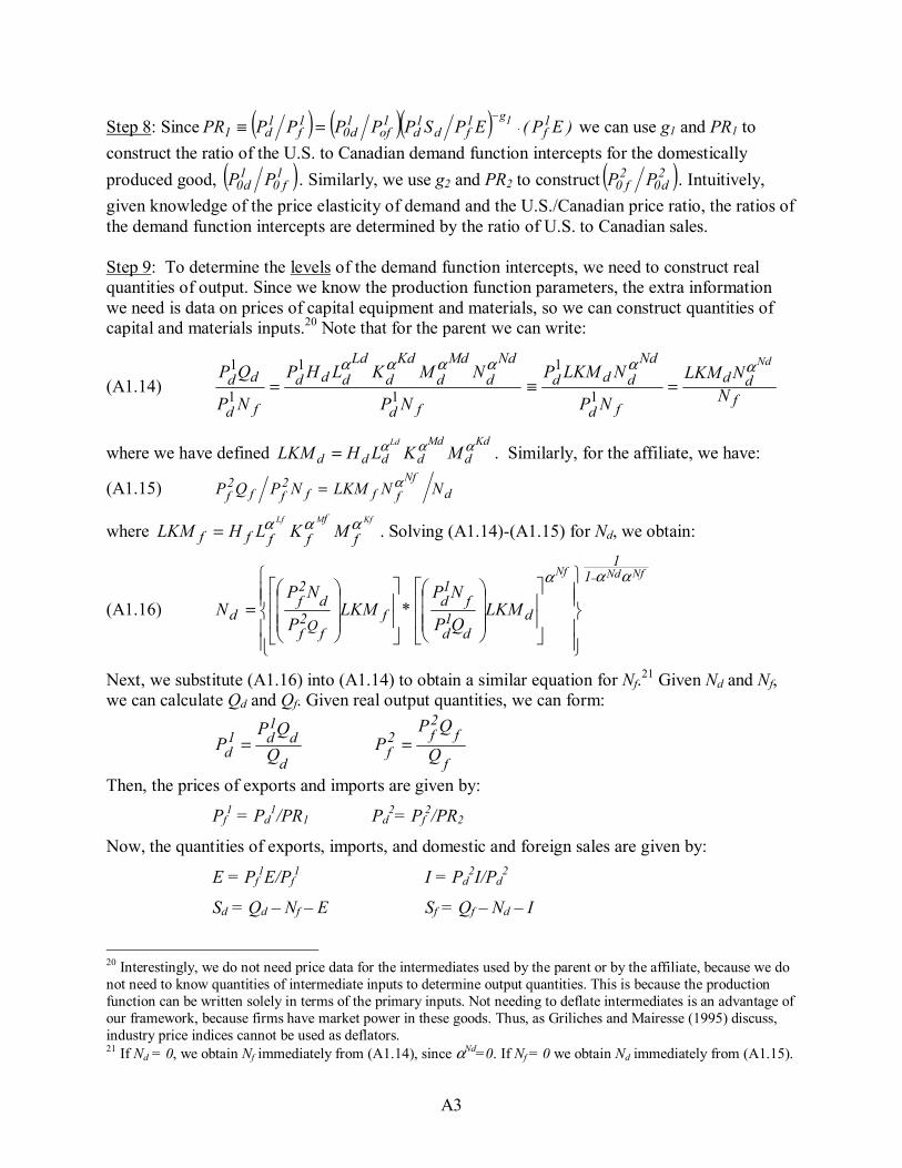
A3

Step 8: Since ( ) ( )( ) )EP(EPSPPPPPPR 1f

1fd

1d

1of

1d0

1f

1d1

1g⋅

−=≡ we can use g1 and PR1 to

construct the ratio of the U.S. to Canadian demand function intercepts for the domestically produced good, ( )1

f01d0 PP . Similarly, we use g2 and PR2 to construct ( )2

d02f0 PP . Intuitively,

given knowledge of the price elasticity of demand and the U.S./Canadian price ratio, the ratios of the demand function intercepts are determined by the ratio of U.S. to Canadian sales. Step 9: To determine the levels of the demand function intercepts, we need to construct real quantities of output. Since we know the production function parameters, the extra information we need is data on prices of capital equipment and materials, so we can construct quantities of capital and materials inputs.20 Note that for the parent we can write:

(A1.14) f

dd

fd

Ndddd

fd

Ndd

Mdd

Kdd

Ldddd

fd

ddN

NLKM

NP

NLKMP

NP

NMKLHP

NP

QPNdαααααα

=≡= 1

1

1

1

1

1

where we have defined KdMd

ddddd MKLHLKMLd ααα= . Similarly, for the affiliate, we have:

(A1.15) dfff2ff

2f NNLKMNPQP

Nfα=

where KfMLf

fffff MKLHLKMf ααα= . Solving (A1.14)-(A1.15) for Nd, we obtain:

(A1.16)

NfNdNf 11

dd

1d

f1d

ffQ2

f

d2f

d LKMQP

NP*LKM

P

NPN

ααα −

=

Next, we substitute (A1.16) into (A1.14) to obtain a similar equation for Nf.21 Given Nd and Nf, we can calculate Qd and Qf. Given real output quantities, we can form:

d

d1d1

d QQP

P = f

f2f2

f Q

QPP =

Then, the prices of exports and imports are given by:

Pf1 = Pd

1/PR1 Pd2= Pf

2/PR2

Now, the quantities of exports, imports, and domestic and foreign sales are given by:

E = Pf1E/Pf

1 I = Pd2I/Pd

2

Sd = Qd – Nf – E Sf = Qf – Nd – I

20 Interestingly, we do not need price data for the intermediates used by the parent or by the affiliate, because we do not need to know quantities of intermediate inputs to determine output quantities. This is because the production function can be written solely in terms of the primary inputs. Not needing to deflate intermediates is an advantage of our framework, because firms have market power in these goods. Thus, as Griliches and Mairesse (1995) discuss, industry price indices cannot be used as deflators. 21 If Nd = 0, we obtain Nf immediately from (A1.14), since αNd=0. If Nf = 0 we obtain Nd immediately from (A1.15).

A4

Finally, we can write the demand function intercepts as:

2

2

g2d

2d0

gf

2f

2f0

IPP

SPP

=

= 1g1

f1f0

gd

1d

1d0

EPP

SPP 1

=

=

In the case that I=0, 2dP and 2

d0P will be undefined, but 2f0P can still be calculated since

dff NQS −= . In the case that E=0, 1fP and 1

f0P will be undefined, but 1d0P can still be calculated

since fdd NQS −= . Step 10: Having obtained the 12 firm specific technology and demand parameters, one can easily map these into the ε vector using the equations of the stochastic specification in section III.

Appendix 2: Identification of H, P0 and R

As discussed in Appendix 1, the sources of identification for the Cobb-Douglas share parameters, price elasticities of demand, and demand function intercept ratios are rather obvious in the context of our model. This is also true of the labor force adjustment cost parameters, which are pinned down by the persistence of employment over time. Much more subtle, however, is the source of identification of the H, P0 and R parameters, which are TFP, the demand intercept levels, and the profit rate. Here we give the intuition for how these parameters are identified.

Regarding TFP, recall that we normalize Ht=1 and t=0 in 1983, and specify that TFP growth is determined by Ht = (1+h)t, where h is an estimated parameter. It is not immediately obvious is how growth in H would be separately identified from changes in the demand function intercepts P0 if output prices and quantities are not separately observed. One might think that, since any observed revenue level can be explained by a locus of price and quantity values, it would be impossible to disentangle H and the P0. However, this is not the case.

Consider a simple autarky case (a single firm with no affiliate), and with K and L as the only inputs, and no adjustment costs. Then we have:

LKLKHQ αα⋅= g

0QPP −= wLKPQ −−= γΠ In this case, labor demand is:

g1

g1

L

K)g1(

0

LK

wHP)g1(w

L

−

=

−

−α

αγαα

Calculating elasticities of labor demand with respect to H and P0, we obtain:

(A2.1) 0g1

PL

LP

0

0 >=∂∂ 0)1(1 >−=

∂∂ g

gHL

LH 0<g<1

Thus, both TFP growth and growth in demand (P0) cause growth in the firm’s employment. If all growth is due to growth in demand, then a firm’s employment growth rate will be inversely proportional to its g. But if all growth is due to TFP growth, then firm growth rates will decline even more quickly with g. In fact, as g→1, the effect of TFP on employment approaches zero. Thus, to the extent that firm employment growth is less than proportional to 1/g (i.e., it is much slower among high g firms), we will conclude that TFP is a bigger factor in growth than P0.

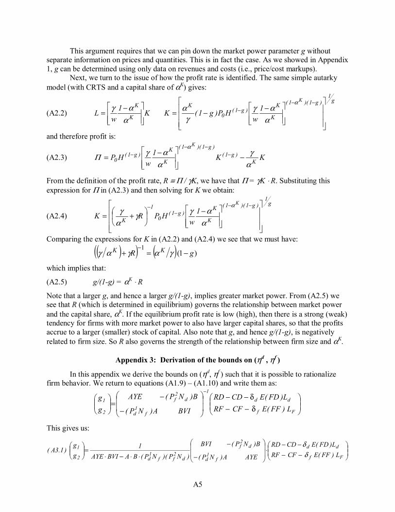
A5

This argument requires that we can pin down the market power parameter g without separate information on prices and quantities. This is in fact the case. As we showed in Appendix 1, g can be determined using only data on revenues and costs (i.e., price/cost markups). Next, we turn to the issue of how the profit rate is identified. The same simple autarky model (with CRTS and a capital share of αK) gives:

(A2.2) K1w

L K

K

−=α

αγ

g1

)g1)(1(

K

K)g1(

0

KK

1w

HP)g1(K

−−=−−

−α

ααγ

γα

and therefore profit is:

(A2.3) KK1w

HP K)g1(

)g1)(1(

K

K)g1(

0

K

αγ

ααγΠ

α

−

−= −−−

−

From the definition of the profit rate, R ≡ Π / γK, we have that Π = γK ⋅ R. Substituting this expression for Π in (A2.3) and then solving for K we obtain:

(A2.4)

g1

)g1)(1(

K

K)g1(

0

1

K

K

1w

HPRK

−

+=−−

−− α

ααγγ

αγ

Comparing the expressions for K in (A2.2) and (A2.4) we see that we must have:

( )( ) ( ) )1(1

gR KK −=+−

γαγαγ

which implies that:

(A2.5) g/(1-g) = αK ⋅ R

Note that a larger g, and hence a larger g/(1-g), implies greater market power. From (A2.5) we see that R (which is determined in equilibrium) governs the relationship between market power and the capital share, αK. If the equilibrium profit rate is low (high), then there is a strong (weak) tendency for firms with more market power to also have larger capital shares, so that the profits accrue to a larger (smaller) stock of capital. Also note that g, and hence g/(1-g), is negatively related to firm size. So R also governs the strength of the relationship between firm size and αK.

Appendix 3: Derivation of the bounds on (ηd , ηf )

In this appendix we derive the bounds on (ηd, ηf ) such that it is possible to rationalize firm behavior. We return to equations (A1.9) – (A1.10) and write them as:

δ−−δ−−

−

−=

−

Ff

dd

1

f1

d

d2f

2

1

L)FF(ECFRFL)FD(ECDRD

BVIA)NP(

B)NP(AYE

gg

This gives us:

−−−−

⋅

−

−

⋅⋅−⋅=

Ff

dd

f1d

d2f

d2ff

1d2

1L)FF(ECFRF

L)FD(ECDRD

AYEA)NP(

B)NP(BVI

)NP)(NP(BABVIAYE1

gg

)1.3A(δ

δ

A6

The term )NP)(NP(BABVIAYE d2ff

1d⋅⋅−⋅ is > 0. Thus, for g1>0 and g2>0, we must have:

0]L)FF(ECFRF[B)NP(]L)FD(ECDRD[BVI ffd2fdd >δ−−+δ−−⋅

0]L)FF(ECFRF[AYE]L)FD(ECDRD[A)NP( ffddf1

d >δ−−+δ−−⋅

Rearranging these expressions, we obtain:

ffd2fddd

2f L)FF(EB)NP(L)FD(EBVI]CFRF[B)NP(]CDRD[BVI)2.3A( δδ +⋅>−+−⋅

ffddf1df

1d L)FF(EAYEL)FD(EA)NP(]CFRF[AYE]CDRD[A)NP()3.3A( δδ +⋅>−+−⋅

Substituting into (A3.2) the definitions of the expectation terms E(FD)Ld and E(FF)Lf (see equation 20) we obtain an expression where the forecast errors ηd and ηf appear explicitly:

]LFF[B)NP(]LFD[BVI]CFRF[B)NP(]CDRD[BVI fffd2fdddd

2f η+⋅δ+η+⋅⋅δ⋅>−+−⋅

If we divide through by BVI > 0 and define BVIB)NP(PDB d2f≡ we obtain:

ffffdddd PDBLFFPDBFDL]CFRF[PDB]CDRD[ ηδ⋅+⋅δ⋅+ηδ+δ>−⋅+−

We can rewrite (A3.3) in a similar way. Then, we obtain the following upper bounds on (ηd, ηf):

BUFLFDPFAFFL]CDRD[PFA]CFRF[PFA

BUDLFFPDBFDL]CFRF[PDB]CDRD[PDB)4.3A(

dffgddff

ffddffdd

≡⋅⋅−−−⋅+−<⋅+

≡⋅⋅−−−⋅+−<⋅+

δδηδηδδδηδηδ

where we have defined ( ) AYEANPPFA f1d≡ . Denoting the upper bounds given by the right

hand sides of the inequalities in (A3.4) by BUD and BUF, we obtain the more compact notation:

(A3.5) ffdd PDB ηδηδ ⋅+ < BUD ddff PFA ηδ⋅+ηδ < BUF

The (ηd, ηf ) vector also has an lower bound, which we can determine from the labor share equations in A(1.13). The requirement αLd>0 gives:

δd E(FD) Ld + wdLd > 0

Substituting the definition of E(FD)Ld we obtain δd (FD·Ld + ηd) + wdLd > 0, which implies the lower bound on ηd:

δd ηd > -wdLd - δd FDLd ≡ BLD

Similarly, for ηf we obtain:

δf ηf > -wfLf - δf FFLf ≡ BLF

Thus, δdηd and δf ηf must satisfy the following four constraints in order for firm behavior to be rationalizable within the model:

(A3.6) BUFPFA

BUDPDB

ddff

ffdd

<⋅+

<⋅+

ηδηδηδηδ

BLFBLD

ff

dd>>

ηδηδ

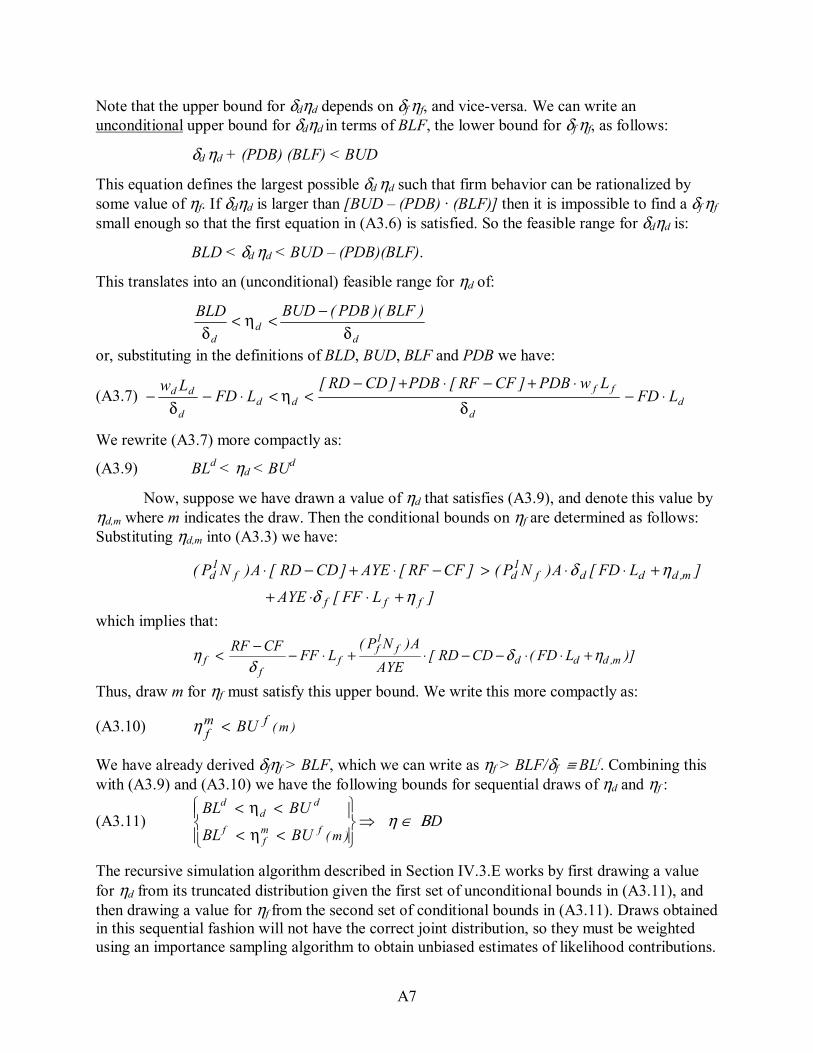
A7

Note that the upper bound for δdηd depends on δf ηf, and vice-versa. We can write an unconditional upper bound for δdηd in terms of BLF, the lower bound for δf ηf, as follows:

δd ηd + (PDB) (BLF) < BUD

This equation defines the largest possible δd ηd such that firm behavior can be rationalized by some value of ηf. If δdηd is larger than [BUD – (PDB) · (BLF)] then it is impossible to find a δf ηf small enough so that the first equation in (A3.6) is satisfied. So the feasible range for δdηd is:

BLD < δd ηd < BUD – (PDB)(BLF).

This translates into an (unconditional) feasible range for ηd of:

dd

d

)BLF)(PDB(BUDBLDδ

−<η<δ

or, substituting in the definitions of BLD, BUD, BLF and PDB we have:

(A3.7) dd

ffdd

d

dd LFDLwPDB]CFRF[PDB]CDRD[

LFDLw

⋅−δ

⋅+−⋅+−<η<⋅−

δ−

We rewrite (A3.7) more compactly as:

(A3.9) BLd < ηd < BUd

Now, suppose we have drawn a value of ηd that satisfies (A3.9), and denote this value by ηd,m where m indicates the draw. Then the conditional bounds on ηf are determined as follows: Substituting ηd,m into (A3.3) we have:

]LFF[AYE

]LFD[A)NP(]CFRF[AYE]CDRD[A)NP(

fff

m,dddf1df

1d

ηδηδ

+⋅⋅+

+⋅⋅>−⋅+−⋅

which implies that:

)]LFD(CDRD[AYE

A)NP(LFFCFRF

m,dddf

1f

ff

f ηδδ

η +⋅⋅−−⋅+⋅−−<

Thus, draw m for ηf must satisfy this upper bound. We write this more compactly as:

(A3.10) )m(fmf BU<η

We have already derived δfηf > BLF, which we can write as ηf > BLF/δf ≡ BLf. Combining this with (A3.9) and (A3.10) we have the following bounds for sequential draws of ηd and ηf :

(A3.11)

<η<

<η<

)m(fmf

f

dd

d

BUBL

BUBL⇒ η ∈ ΒD

The recursive simulation algorithm described in Section IV.3.E works by first drawing a value for ηd from its truncated distribution given the first set of unconditional bounds in (A3.11), and then drawing a value for ηf from the second set of conditional bounds in (A3.11). Draws obtained in this sequential fashion will not have the correct joint distribution, so they must be weighted using an importance sampling algorithm to obtain unbiased estimates of likelihood contributions.