Embed Size (px)
Citation preview
Smooth Path Planning using Biclothoid Fillets for High Speed CNC MachinesI
Abbas Shahzadeha, Abbas Khosravia, Troy Robinetteb, Saeid Nahavandia
aDeakin University, 75 Pigdons Road, Waurn Ponds VIC 3216, AustraliabANCA Motion, 1 Bessemer Rd, Bayswater North VIC 3153, Australia
Abstract
In high speed Computer Numerical Control (CNC) machines, cut velocities greater than 60 metres per minute andaccelerations higher than 2g are used. In such high feedrates and accelerations, even a small discontinuity in curvatureor in tangency can result in jerk spikes and consequently in machine vibrations, poor cut quality and decreased lifespanof the equipment. To prevent these consequences, using path smoothing techniques is necessary. Many path smoothingmethods have been proposed in the literature to eliminate toolpath discontinuities. However the usage of almost all ofthese techniques is limited to purely linear toolpaths. In this paper a new path smoothing method using biclothoid filletsis introduced. The proposed method can be used to convert any given path consisted of lines and arcs to a curvaturecontinuous path. The generated path is arc length parameterised which makes it easy to interpolate. The distancebetween the G2-continuous path and the original toolpath is limited to an adjustable tolerance. The proposed methodhas been tested on a CNC laser cutting machine and the results are reported. The main contribution of this paper is afillet fitting method which is not limited to line to line transitions. The proposed smoothing fillets can be fitted betweentwo arcs or a line and arc as well. A comparison with Bezier fillets, shows that using the proposed method results in asmoother curvature profile, higher feedrates and shorter cycle times.
Keywords:CNC, path planning, corner smoothing, jerk, G2 continuity, clothoid
1. Introduction
Standard part programs processed by CNC controllers,define toolpaths which are composed of several lines andarcs [1]. At each line to line, line to arc or arc to arc transi-tion, careful considerations are required to ensure that thephysical limits of the machine are not exceeded. For exam-ple when the machine is moving at a constant feedrate, atthe point where two successive non-tangent linear movesmeet, there will be a sudden change in the velocity of theparticipating joints. Therefore, the controller has to fore-see these transition points and reduce the path velocity tolimit the side effects of a step change in the velocity. Sim-ilarly at line to arc and arc to arc transitions, even whenthe two moves are completely tangent, curvature discon-tinuities have to be addressed. Any discontinuity in thecurvature results in a step change in acceleration and con-sequently in a jerk spike which can have detrimental effectson the quality of cut.
The same issue needs to be addressed in path planningfor mobile robots and also in highway and railway design.
IThis manuscript has been accepted in International Journal ofMachine Tools and Manufacture. For the final document please referto: https://doi.org/10.1016/j.ijmachtools.2018.04.003
Email addresses: [email protected]
(Abbas Shahzadeh), [email protected] (AbbasKhosravi), [email protected] (Troy Robinette),[email protected] (Saeid Nahavandi)
The problem can be explained in a more tangible way inthe context of wheeled vehicles. Imagine a car which isbeing driven on a road. For moving on a straight line, theangle of the front wheels with the chassis of the car needsto be zero. However for turning on a circular bend with aradius equal to 15 metres, for a typical car, the angle of thefront wheels has to be about 10 degrees. In a non-standardroad where a straight line segment is immediately followedby a circular bend, the driver will have to change the angleof the front wheels from zero to 10 degrees instantaneouslywhich is physically impossible. So in order to follow theroad, the car has to stop, reorient its front wheels and startmoving again [2]. To prevent cases like the given example,smoothing curves like clothoids are used in highway andrailway design. The role of the smoothing curves is toprevent sudden changes in the curvature and to eliminatecurvature discontinuities.
In the case of CNC machines, there are two modesof operation known as Exact Stop Mode and Continu-ous Mode [1]. In the Exact Stop Mode, discontinuitiesin the toolpath do not make any difference in the overallperformance. The reason is that in this mode, the ma-chine stops after each move and before starting the nextmove. However in the Continuous Mode, in order to have ajerk-limited smooth movement, planning a curvature con-tinuous path without any discontinuities in curvature ortangency is necessary.
Preprint submitted to International Journal of Machine Tools and Manufacture 1.4.2018
As mentioned before, the same problem has been stud-ied for mobile robots and autonomous vehicles [2, 3, 4, 5].However, CNC applications have an important additionalrequirement that needs to be considered in path smooth-ing. In these applications, the accuracy of the travelledpath has to be maintained. To satisfy this requirement,the deviation introduced by the smoothing algorithm hasto be limited. In other words the maximum distance be-tween the smoothed path and the original path should bewithin a specified tolerance.
The rest of this paper is organized as follows. In sec-tion 2, the related work is discussed and the gaps in theliterature which this paper is trying to fulfil are briefly ex-plained. In section 3 the problem that this paper is tryingto solve is outlined using a sample part program. A shortintroduction to clothoids is given in section 4. Section 5,introduces biclothoid fillets which are the fillets used forcorner smoothing in this paper. Methods and algorithmsused for fitting biclothoid fillets at line to line, line to arcor arc to arc transitions are explained in section 6. Sec-tion 7 covers the methods used in this work for measuringand limiting the maximum distance between the smoothedpath and the original path. Formulas for calculating themaximum acceleration and jerk when moving on a clothoidand the maximum permissible velocity are given in section8. This section is followed by a case study in section 9.In section 10, the proposed method is compared with themethod from [6]. Finally section 11, concludes the paper.
2. Related Work
Papers discussing the problem of path smoothing forCNC machines can be divided into two main categories.In the first group of papers, methods for finding smoothsplines that pass through a large number of input pointsare proposed [7, 8, 9]. Spline fitting is used when thetoolpath is composed of a large number of small linearsegments (also known as micro-lines). The second group ofpapers, discuss the problem of corner smoothing. Cornersmoothing is used when the moves generated by the CAD-CAM software are longer (in comparison to micro-lineswhich are better smoothed using splines) and can be eitherlines or arc segments. This work falls in the latter category.
Several methods are proposed for corner smoothing inthe literature. Polynomial curve splines are used as tran-sition curves in some works. Erkorkmaz et al. in [10],use quintic splines composed of two or three quintic splinesegments as smooth transition curves. The choice betweentwo or three segments depends on the type of the servocontrollers used in the machine. To get near arc lengthparameterisation, the authors of [10] use the method pro-posed by Yang and Wang in [11]. Despite using the men-tioned technique for near arc length parameterisation, ve-locity discontinuities still exist in the generated spline [10]which have to be resolved by using special interpolationtechniques [10, 12].
Yutkowitz in [13] uses two back to back quartic poly-nomials per axis to round the corners. For each corner,the curvature of the smoothing curve becomes maximumat the middle of the fillet where the two quartic curvesjoin. In order to decrease feedrate fluctuations the valueof the maximum curvature for each corner is optimised sothat the polynomial parameter is close to the arc length.In other words, the smoothing curve is nearly arc lengthparameterised.
Beudaert et al. in [14] use cubic splines. They smootheach joint separately by fitting a cubic spline to the po-sition stream and then measure the resulting geometricdeviation. An optimisation algorithm tries to maximisethe feedrate while keeping the introduced error below aspecified tolerance.
Bezier curves are also used for corner smoothing. Yangand Sukkarieh in [15] use two back to back cubic Beziercurves to generate smooth transitions from a line to an-other line at the corners. Their method is intended formobile robots and generates a continuous curvature pathwith an upper bound limit on curvature. In the intendedapplication, the path deviation is not important and is nottaken into account.
Sencer et al. in [6] also use Bezier curves to smoothline to line transitions. Instead of using two cubic Beziercurves, one quintic Bezier curve is used. They have de-vised a method to generate a smoothing curve with min-imum curvature peak for any corner angle. They showthat by decreasing the maximum curvature of the transi-tion curve, higher feedrates can be achieved. Since Beziercurves are not arc length parameterised, a special interpo-lation method has to be used in order to prevent feedratefluctuations [6, 15].
Bi et al. in [16] and [17] use a particular type of cu-bic Bezier curves first introduced in [18]. In [18], Waltonand Meek, use cubic Bezier curves which normally havefour control points. However, they merge two of the con-trol points and place them at the corner. This ensuresthat the curvature profile of the Bezier curve has only oneextremum at the middle of the curve [18]. Walton andMeek do not attempt to limit the deviation between thesmoothing Bezier curve and the original curve. Bi et al.in [16] and [17], however, measure and limit the deviationto make sure that it is bounded to a predefined value.
Fan et al. in [19] use two back to back quartic Beziercurves to achieve G3 continuity. Each of the Bezier curveshas 5 control points and the two back to back curves shareone control point which leaves 9 control points to calcu-late. In determining the control points, they minimise thecurvature variation energy (CVE) [19] in order to minimisethe cycle time and improve the smoothness.
B-spline curves are also used as path smoothing fillets.Zhao et al. in [20] use cubic B-splines with 5 control points.By dividing the B-spline into two cubic Bezier curves theyprove that the maximum curvature falls exactly in the mid-dle of the B-spline. They limit the feedrate based on themaximum curvature of the smoothing B-spline.
2
Beudaert et al. in [21] also use cubic B-splines with 5control points where the third control point is placed atthe corner. Since there are three points on each line of thecorner, the curvature at the beginning and at the end ofthe smoothing curve is zero which matches the curvaturesof the comprising lines. They explain that the distancebetween control points can be adjusted in order to min-imise the machining time. However, they also give a ruleof thumb and state that if the distance between the firstcontrol point and the corner is 1.4 to 1.75 times largerthan the distance between the second control point andthe corner, satisfying results in terms of machining timecan be achieved.
Tulsyan and Altintas in [22] and also Yang and Yuen in[23] use quintic B-splines with 7 control points in order toachieve G3 continuity. One of the 7 control points is placedat the corner so that there are four control points on eachline of the corner. This arrangement results in zero curva-ture and also a zero derivative of curvature at the begin-ning and at the end of the smoothing curve. Their methodis designed for smoothing corners in a 5-axis milling ma-chine. Tulsyan and Altintas in [22] use a septic B-splinewith 9 control points for smoothing the orientation.
Pythagorean-hodograph (PH) curves are another groupof curves used for corner smoothing. Shi et al. in [24] usethe method first introduced in [18]. They use a quinticPH curve which has 6 control points. The second andthird control points are merged and also the fourth andfifth control points are merged to ensure a single curva-ture extremum on the curve. They extract an analyticalexpression for the maximum curvature of the smoothingcurve.
Another method of corner smoothing proposed in [25]and [26] by Tajima and Sencer, uses a single step solution.It should be noted that in most of the algorithms for cornersmoothing, at first a smoothing curve is fitted to replacethe corner, and then the smoothed path is interpolated.In contrast to the common method, Tajima and Sencerpropose smoothing the corner by directly calculating andcontrolling the jerk, acceleration and velocity when thetoolpath is being interpolated. In [25] they explain theiralgorithm for a 3-axis machine. Using the proposed algo-rithm, the jerk of one of the joints is always at its maximumto ensure that the smoothing time is minimised. In [26]they extend their algorithm to a 5-axis case.
This paper, uses biclothoid fillets (two back to backclothoids) as transition curves to smooth the corners andeliminate discontinuities in the toolpath. Clothoids havebeen used in path planning for mobile robots. Shin et al.in [4], use three clothoids to connect every two successivepoints while matching the tangency and curvature at bothends. Since the intended application is path planning forrobots, the deviation between the original path and thegenerated path is not limited [4]. Brezak and Petrovic in[5], use two clothoids for corner smoothing. They studyboth line to line and arc to line cases while always assumingzero curvature at one end. The reason for this assumption
is that robots mainly move on straight lines. However, thisassumption is not valid for CNC machines.
Shahzadeh et al. in [7], use clothoids to generate aG2-continuous clothoid spline with limited deviation fromthe original toolpath for CNC applications. However, theproposed method can only handle toolpaths that are sym-metrical and G1-continuous. In other words, similar to theother works referenced in this section, the method in [7],cannot be used to smooth general line to arc or arc to arcdiscontinuities.
Clothoids have a number of advantages over other curvesfor corner smoothing which will be explained in the com-ing sections of this paper. However, they have not beenwidely used in CNC applications. The main concern forusing clothoids in CNC applications is the computation in-tensity [15]. In order to interpolate a clothoid, calculationof Fresnel integrals is necessary and unfortunately theseintegrals do not have a closed form solution. Nevertheless,Fresnel integrals can be accurately (with error smaller than4× 10−8) estimated using a few rational polynomials [27].A clothoid can also be interpolated using a look up tablein real time applications with limited CPU power [28]. Us-ing either of the mentioned techniques, the computationalintensity issue can be resolved.
The main limitation of the works referenced above (ex-cept for [4] and [5] which are not intended for CNC appli-cations) is that they only discuss line to line transitions.However, in practice, part programs are consisted of bothlinear and helical (or arc) moves.
Another limitation when using polynomial curves, B-splines or Bezier curves is that for these curves, the arclength cannot be calculated using an analytical formula.For these curves, the arc length can only be estimated byintegration [15, 24]. Not having an accurate arc lengthresults in feedrate fluctuations [29, 30, 31]. Special inter-polators are needed to decrease the feedrate fluctuationswhen using parametric curves. For example [9] and [32]use one or more 9th degree polynomials as feedrate cor-rection functions to compensate for the lack of arc lengthparameterisation. Kinematic corner smoothing methodsproposed in [25, 26] have the same problem.
PH curves have the advantage that their arc lengthcan be calculated analytically for any value of the curveparameter. However, despite the fact that PH curves havean analytical arc length, they are not arc length parame-terised. As a result again special interpolators are neces-sary to process these curves [33, 34].
Finally in majority of the papers referenced above,only maximum curvature is considered when calculatingthe maximum permissible feedrate. Also in some papers,in order to increase the feedrate, the maximum curvaturehas been minimised. Nevertheless, in section 8 it will beproved that for calculating the maximum permissible fee-drate, the derivative of curvature (sharpness) is just asimportant as the curvature itself.
3
−20 0 20 40
0
20
40
60
O
A
B
C
X (mm)
Y(m
m)
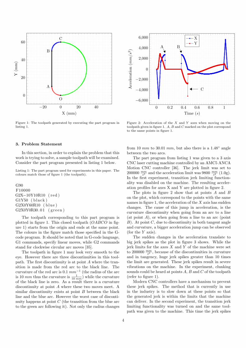
Figure 1: The toolpath generated by executing the part program inlisting 1.
3. Problem Statement
In this section, in order to explain the problem that thiswork is trying to solve, a sample toolpath will be examined.Consider the part program presented in listing 1 below.
Listing 1: The part program used for experiments in this paper. Thecolours match those of figure 1 (the toolpath).
G90F10000G2X−10Y10R10 ( red )G1Y50 ( black )G2X0Y60R10 ( blue )G2X0Y0R30.01 ( green )
The toolpath corresponding to this part program isplotted in figure 1. This closed toolpath (OABCO in fig-ure 1) starts from the origin and ends at the same point.The colours in the figure match those specified in the G-code program. It should be noted that in G-code language,G1 commands, specify linear moves, while G2 commandsstand for clockwise circular arc moves [35].
The toolpath in figure 1 may look very smooth to theeye. However there are three discontinuities in this tool-path. The first discontinuity is at point A where the tran-sition is made from the red arc to the black line. Thecurvature of the red arc is 0.1 mm−1 (the radius of the arcis 10 mm thus the curvature is 1
10 mm ) while the curvatureof the black line is zero. As a result there is a curvaturediscontinuity at point A where these two moves meet. Asimilar discontinuity exists at point B between the blackline and the blue arc. However the worst case of disconti-nuity happens at point C (the transition from the blue arcto the green arc following it). Not only the radius changes
0 0.2 0.4 0.6 0.8 1
−6,000
−4,000
−2,000
0
2,000
4,000
6,000
A B
C
Time (s)
Acc
eler
ati
on(mm/s2
)
XY
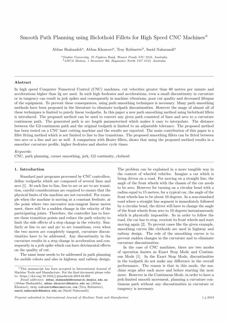
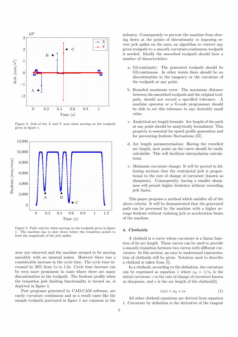
Figure 2: Acceleration of the X and Y axes when moving on thetoolpath given in figure 1. A, B and C marked on the plot correspondto the same points in figure 1.
from 10 mm to 30.01 mm, but also there is a 1.48 anglebetween the two arcs.
The part program from listing 1 was given to a 3 axisCNC laser cutting machine controlled by an AMC5 ANCAMotion CNC controller [36]. The jerk limit was set to200000 mm
s3 and the acceleration limit was 9800 mms2 (1.0g).
In the first experiment, transition jerk limiting function-ality was disabled on the machine. The resulting acceler-ation profiles for axes X and Y are plotted in figure 2.
The plots in figure 2 show that at points A and Bon the plot, which correspond to the points with the samenames in figure 1, the acceleration of theX axis has suddenchanges. The cause of this jump in acceleration, is thecurvature discontinuity when going from an arc to a line(at point A), or when going from a line to an arc (pointB). At point C, due to discontinuity in both tangent angleand curvature, a bigger acceleration jump can be observed(for the Y axis).
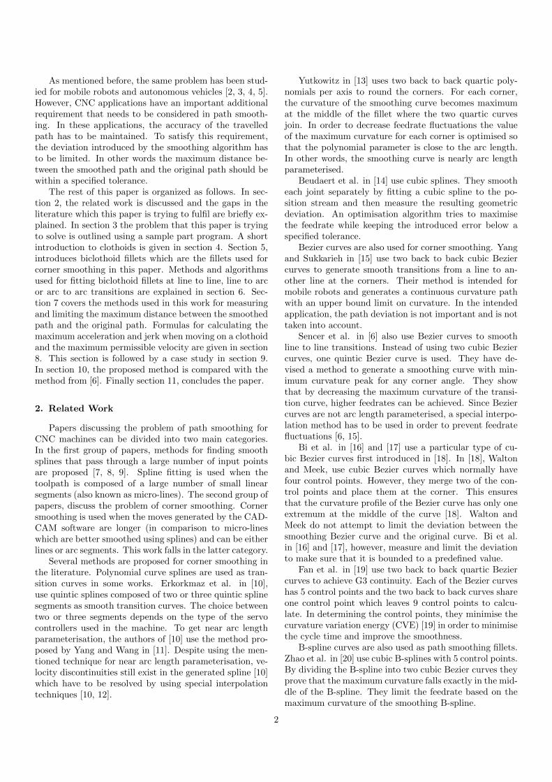
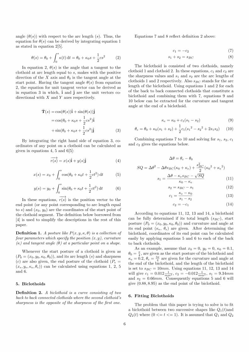
The sudden changes in the acceleration translate tobig jerk spikes as the plot in figure 3 shows. While thejerk limits for the axes X and Y of the machine were setto 200000 mm
s3 , because of the discontinuities in curvatureand in tangency, huge jerk spikes greater than 10 timesthe limit are generated. These jerk spikes result in severevibrations on the machine. In the experiment, clunkingsounds could be heard at points A, B and C of the toolpath(refer to figure 1).
Modern CNC controllers have a mechanism to preventthese jerk spikes. The method that is currently in usein the industry is to slow down at these points so thatthe generated jerk is within the limits that the machinecan deliver. In the second experiment, the transition jerklimiting functionality was turned on and the same tool-path was given to the machine. This time the jerk spikes
4
0 0.2 0.4 0.6 0.8 1
−2
−1
0
1
2
3·106
A
B
C
Time (s)
Jer
k(mm/s
3)
XY
Figure 3: Jerk of the X and Y axes when moving on the toolpathgiven in figure 1.
0 0.2 0.4 0.6 0.8 1 1.2
0
2,000
4,000
6,000
8,000
10,000
12,000
A B
C
Time (s)
Fee
dra
te(mm/m
in)
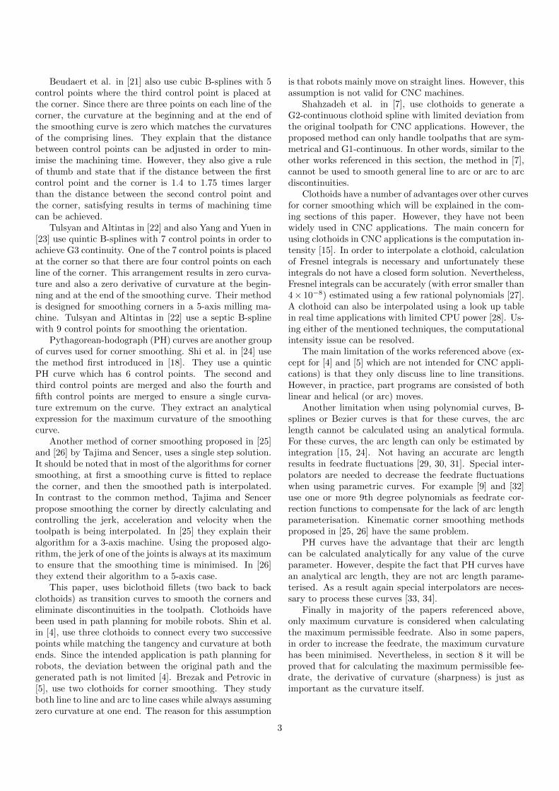
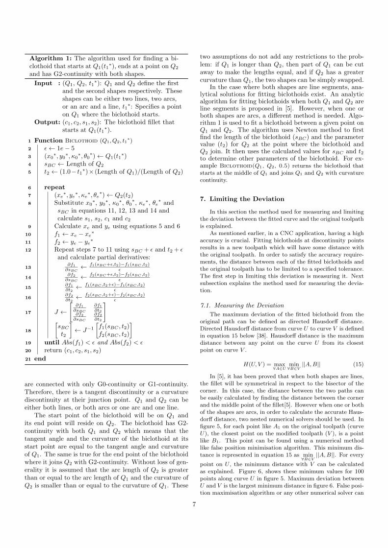
Figure 4: Path velocity when moving on the toolpath given in figure1. The machine has to slow down before the transition points tolimit the magnitude of the jerk spikes.
were not observed and the machine seemed to be movingsmoothly with no unusual noises. However there was aconsiderable increase in the cycle time. The cycle time in-creased by 20% from 1s to 1.2s. Cycle time increase canbe even more prominent in cases where there are manydiscontinuities in the toolpath. The feedrate profile whenthe transition jerk limiting functionality is turned on, isdepicted in figure 4.
Part programs generated by CAD-CAM software, arerarely curvature continuous and as a result cases like thesample toolpath portrayed in figure 1 are common in the
industry. Consequently to prevent the machine from slow-ing down at the points of discontinuity or imposing se-vere jerk spikes on the axes, an algorithm to convert anygiven toolpath to a smooth curvature-continuous toolpathis needed. Ideally the smoothed toolpath should have anumber of characteristics:
a. G2-continuity: The generated toolpath should beG2-continuous. In other words there should be nodiscontinuities in the tangency or the curvature ofthe toolpath at any point.
b. Bounded maximum error: The maximum distancebetween the smoothed toolpath and the original tool-path, should not exceed a specified tolerance. Amachine operator or a G-code programmer shouldbe able to set this tolerance to any desirably smallvalue.
c. Analytical arc length formula: Arc length of the pathat any point should be analytically formulated. Thisproperty is essential for speed profile generation andfor preventing feedrate fluctuations [37].
d. Arc length parameterisation: Having the travelledarc length, next point on the curve should be easilycalculable. This will facilitate interpolation calcula-tions.
e. Minimum curvature change: It will be proved in fol-lowing sections that the centripetal jerk is propor-tional to the rate of change of curvature (known assharpness). Consequently, having a smaller sharp-ness will permit higher feedrates without exceedingjerk limits.
This paper proposes a method which satisfies all of theabove criteria. It will be demonstrated that the generatedpath can be processed by the machine with a higher av-erage feedrate without violating jerk or acceleration limitsof the machine.
4. Clothoids
A clothoid is a curve whose curvature is a linear func-tion of its arc length. These curves can be used to providea smooth transition between two curves with different cur-vatures. In this section, an easy to understand representa-tion of clothoids will be given. Notation used to describea clothoid is taken from [5].
In a clothoid, according to the definition, the curvaturecan be expressed as equation 1 where κ0 = 1/r0 is theinitial curvature, c is the rate of change of curvature knownas sharpness, and s is the arc length of the clothoid[5].
κ(s) = κ0 + cs (1)
All other clothoid equations are derived from equation1. Curvature by definition is the derivative of the tangent
5
angle (θ(s)) with respect to the arc length (s). Thus, theequation for θ(s) can be derived by integrating equation 1as stated in equation 2[5].
θ(s) = θ0 +
∫ s
0
κ(t) dt = θ0 + κ0s+1
2cs2 (2)
In equation 2, θ(s) is the angle that a tangent to theclothoid at arc length equal to s, makes with the positivedirection of the X axis and θ0 is the tangent angle at thestart point. Having the tangent angle θ(s) from equation2, the equation for unit tangent vector can be derived asin equation 3 in which, i and j are the unit vectors co-directional with X and Y axes respectively.
T(s) = cos(θ(s))i + sin(θ(s))j
= cos(θ0 + κ0s+1
2cs2)i
+ sin(θ0 + κ0s+1
2cs2)j (3)
By integrating the right hand side of equation 3, co-ordinates of any point on a clothoid can be calculated asgiven in equations 4, 5 and 6[5]:
−−→r(s) = x(s)i + y(s)j (4)
x(s) = x0 +
∫ s
0
cos(θ0 + κ0t+1
2ct2) dt (5)
y(s) = y0 +
∫ s
0
sin(θ0 + κ0t+1
2ct2) dt (6)
In these equations,−−→r(s) is the position vector to the
end point (or any point corresponding to arc length equalto s) and (x0, y0) are the coordinates of the start point ofthe clothoid segment. The definition below borrowed from[4] is used to simplify the descriptions in the rest of thispaper.
Definition 1. A posture like P (x, y, κ, θ) is a collection offour parameters which specify the position (x, y), curvature(κ) and tangent angle (θ) at a particular point on a shape.
Whenever the start posture of a clothoid is given as(P0 = (x0, y0, κ0, θ0)), and its arc length (s) and sharpness(c) are also given, the end posture of the clothoid (Pe =(xe, ye, κe, θe)) can be calculated using equations 1, 2, 5and 6.
5. Biclothoids
Definition 2. A biclothoid is a curve consisting of twoback to back connected clothoids where the second clothoid’ssharpness is the opposite of the sharpness of the first one.
Equations 7 and 8 reflect definition 2 above:
c1 = −c2 (7)
s1 + s2 = sBC (8)
The biclothoid is consisted of two clothoids, namelyclothoid 1 and clothoid 2. In these equations, c1 and c2 arethe sharpness values and s1 and s2 are the arc lengths ofclothoids 1 and 2 respectively. Also sBC stands for the arclength of the biclothoid. Using equations 1 and 2 for eachof the back to back connected clothoids that constitute abiclothoid and combining them with 7, equations 9 and10 below can be extracted for the curvature and tangentangle at the end of a biclothoid.
κe = κ0 + c1(s1 − s2) (9)
θe = θ0 + κ0(s1 + s2) +1
2c1(s1
2 − s22 + 2s1s2) (10)
Combining equations 7 to 10 and solving for s1, s2, c1and c2 gives the equations below.
∆θ = θe − θ0
SQ = ∆θ2 −∆θsBC(κ0 + κe) +s2BC
2(κ0
2 + κe2)
s1 =∆θ − κesBC −
√SQ
κ0 − κe(11)
s2 = sBC − s1 (12)
c1 =κe − κ0s1 − s2
(13)
c2 = −c1 (14)
According to equations 11, 12, 13 and 14, a biclothoidcan be fully determined if its total length (sBC), startposture (P0 = (x0, y0, κ0, θ0)) and curvature and angle atits end point (κe, θe) are given. After determining thebiclothoid, coordinates of its end point can be calculatedeasily by applying equations 5 and 6 to each of the backto back clothoids.
As an example, assume that x0 = 0, y0 = 0, κ0 = 0.1,θ0 = π
4 , are given as the start posture of the biclothoid andκe = 0.2, θe = 3π
4 are given for the curvature and angle atthe end of the biclothoid, and the length of the biclothoidis set to sBC = 10mm. Using equations 11, 12, 13 and 14will give c1 = 0.012 1
mm2 , c2 = −0.012 1mm2 , s1 = 9.34mm
and s2 = 0.66mm. Consequently equations 5 and 6 willgive (0.88, 8.95) as the end point of the biclothoid.
6. Fitting Biclothoids
The problem that this paper is trying to solve is to fita biclothoid between two successive shapes like Q1(t)andQ2(t) where (0 <= t <= 1). It is assumed that Q1 and Q2
6
Algorithm 1: The algorithm used for finding a bi-clothoid that starts at Q1(t1
∗), ends at a point on Q2
and has G2-continuity with both shapes.
Input : (Q1, Q2, t1∗): Q1 and Q2 define the first
and the second shapes respectively. Theseshapes can be either two lines, two arcs,or an arc and a line, t1
∗: Specifies a pointon Q1 where the biclothoid starts.
Output: (c1, c2, s1, s2): The biclothoid fillet thatstarts at Q1(t1
∗).
1 Function Biclothoid (Q1, Q2, t1∗)
2 ε← 1e− 53 (x0
∗, y0∗, κ0
∗, θ0∗)← Q1(t1
∗)4 sBC ← Length of Q2
5 t2 ← (1.0− t1∗)× (Length of Q1)/(Length of Q2)
6 repeat7 (xe
∗, ye∗, κe
∗, θe∗)← Q2(t2)
8 Substitute x0∗, y0
∗, κ0∗, θ0
∗, κe∗, θe
∗ andsBC in equations 11, 12, 13 and 14 andcalculate s1, s2, c1 and c2
9 Calculate xe and ye using equations 5 and 610 f1 ← xe − xe∗11 f2 ← ye − ye∗12 Repeat steps 7 to 11 using sBC + ε and t2 + ε
and calculate partial derivatives:
13∂f1∂sBC
← f1(sBC+ε,t2)−f1(sBC ,t2)ε
14∂f2∂sBC
← f2(sBC+ε,t2)−f2(sBC ,t2)ε
15∂f1∂t2← f1(sBC ,t2+ε)−f1(sBC ,t2)
ε
16∂f2∂t2← f2(sBC ,t2+ε)−f2(sBC ,t2)
ε
17 J ←
[∂f1∂sBC
∂f1∂t2
∂f2∂sBC
∂f2∂t2
]18
[sBCt2
]← J−1
[f1(sBC , t2)f2(sBC , t2)
]19 until Abs(f1) < ε and Abs(f2) < ε20 return (c1, c2, s1, s2)
21 end
are connected with only G0-continuity or G1-continuity.Therefore, there is a tangent discontinuity or a curvaturediscontinuity at their junction point. Q1 and Q2 can beeither both lines, or both arcs or one arc and one line.
The start point of the biclothoid will be on Q1 andits end point will reside on Q2. The biclothoid has G2-continuity with both Q1 and Q2 which means that thetangent angle and the curvature of the biclothoid at itsstart point are equal to the tangent angle and curvatureof Q1. The same is true for the end point of the biclothoidwhere it joins Q2 with G2-continuity. Without loss of gen-erality it is assumed that the arc length of Q2 is greaterthan or equal to the arc length of Q1 and the curvature ofQ2 is smaller than or equal to the curvature of Q1. These
two assumptions do not add any restrictions to the prob-lem: if Q1 is longer than Q2, then part of Q1 can be cutaway to make the lengths equal, and if Q2 has a greatercurvature than Q1, the two shapes can be simply swapped.
In the case where both shapes are line segments, ana-lytical solutions for fitting biclothoids exist. An analyticalgorithm for fitting biclothoids when both Q1 and Q2 areline segments is proposed in [5]. However, when one orboth shapes are arcs, a different method is needed. Algo-rithm 1 is used to fit a biclothoid between a given point onQ1 and Q2. The algorithm uses Newton method to firstfind the length of the biclothoid (sBC) and the parametervalue (t2) for Q2 at the point where the biclothoid andQ2 join. It then uses the calculated values for sBC and t2to determine other parameters of the biclothoid. For ex-ample Biclothoid(Q1, Q2, 0.5) returns the biclothoid thatstarts at the middle of Q1 and joins Q1 and Q2 with curvaturecontinuity.
7. Limiting the Deviation
In this section the method used for measuring and limitingthe deviation between the fitted curve and the original toolpathis explained.
As mentioned earlier, in a CNC application, having a highaccuracy is crucial. Fitting biclothoids at discontinuity pointsresults in a new toolpath which will have some distance withthe original toolpath. In order to satisfy the accuracy require-ments, the distance between each of the fitted biclothoids andthe original toolpath has to be limited to a specified tolerance.The first step in limiting this deviation is measuring it. Nextsubsection explains the method used for measuring the devia-tion.
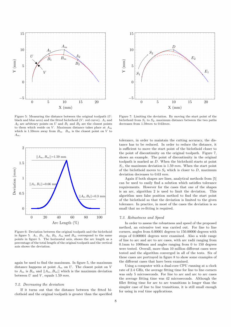
7.1. Measuring the Deviation
The maximum deviation of the fitted biclothoid from theoriginal path can be defined as directed Hausdorff distance.Directed Hausdorff distance from curve U to curve V is definedin equation 15 below [38]. Hausdorff distance is the maximumdistance between any point on the curve U from its closestpoint on curve V .
H(U, V ) = max∀A∈U
min∀B∈V
||A,B|| (15)
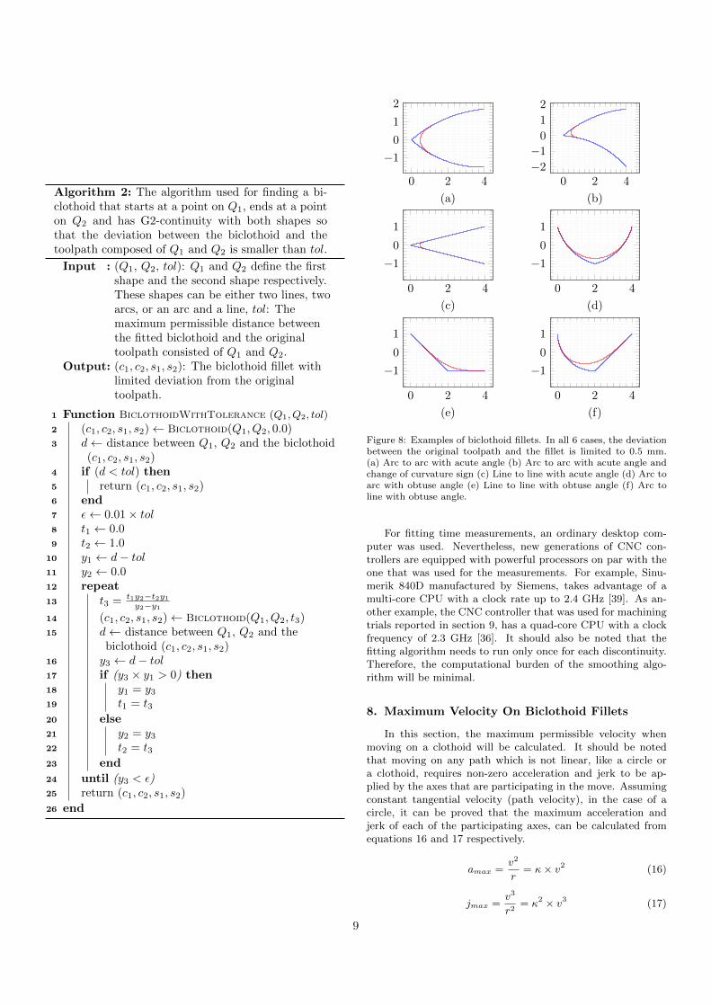
In [5], it has been proved that when both shapes are lines,the fillet will be symmetrical in respect to the bisector of thecorner. In this case, the distance between the two paths canbe easily calculated by finding the distance between the cornerand the middle point of the fillet[5]. However when one or bothof the shapes are arcs, in order to calculate the accurate Haus-dorff distance, two nested numerical solvers should be used. Infigure 5, for each point like A1 on the original toolpath (curveU), the closest point on the modified toolpath (V ), is a pointlike B1. This point can be found using a numerical methodlike false position minimisation algorithm. This minimum dis-tance is represented in equation 15 as min
∀B∈V||A,B||. For every
point on U , the minimum distance with V can be calculatedas explained. Figure 6, shows these minimum values for 100points along curve U in figure 5. Maximum deviation betweenU and V is the largest minimum distance in figure 6. False posi-tion maximisation algorithm or any other numerical solver can
7
0 5 10 15 20−5
0
5
10
15
U
V
A1
B1
Am
BmA2
B2
X (mm)
Y(m
m)
Figure 5: Measuring the distance between the original toolpath (U :black and blue arcs) and the fitted biclothoid (V : red curve). A1 andA2 are arbitrary points on U and B1 and B2 are the closest pointsto them which reside on V . Maximum distance takes place at Am
which is 1.59mm away from Bm. Bm is the closest point on V toAm.
0 20 40 60 80 100
0
0.5
1
1.5
2
||A1, B1||=0.66 mm
||Am, Bm||=1.59 mm
||A2, B2||=0.3 mm
Arc Length (%)
Dev
iati
on(mm
)
Figure 6: Deviation between the original toolpath and the biclothoidin figure 5. A1, B1, A2, B2, Am and Bm correspond to the samepoints in figure 5. The horizontal axis, shows the arc length as apercentage of the total length of the original toolpath and the verticalaxis shows the deviation.
again be used to find the maximum. In figure 5, the maximumdistance happens at point Am on U . The closest point on Vto Am is Bm and ||Am, Bm|| which is the maximum deviationbetween U and V , equals 1.59 mm.
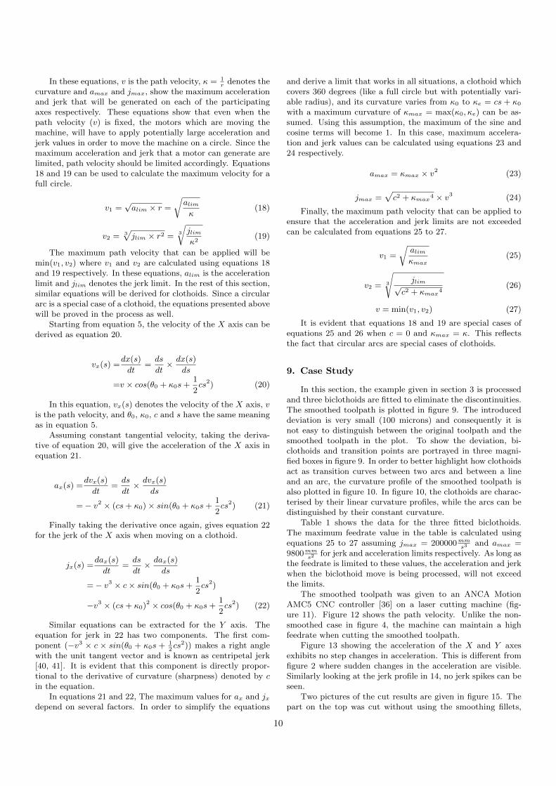
7.2. Decreasing the deviation
If it turns out that the distance between the fitted bi-clothoid and the original toolpath is greater than the specified
0 5 10 15 20−5
0
5
10
15
D
S1E1
S2
E2
X (mm)
Y(m
m)
Figure 7: Limiting the deviation. By moving the start point of thebiclothoid from S1 to S2, maximum distance between the two pathsdecreases from 1.59mm to 0.63mm.
tolerance, in order to maintain the cutting accuracy, the dis-tance has to be reduced. In order to reduce the distance, itis sufficient to move the start point of the biclothoid closer tothe point of discontinuity on the original toolpath. Figure 7,shows an example. The point of discontinuity in the originaltoolpath is marked as D. When the biclothoid starts at pointS1, the maximum deviation is 1.59 mm. When the start pointof the biclothoid moves to S2 which is closer to D, maximumdeviation decreases to 0.63 mm.
Again if both shapes are lines, analytical methods from [5]can be used to easily find a solution which satisfies tolerancerequirements. However for the cases that one of the shapesis an arc, algorithm 2 is used to limit the deviation. Thisalgorithm uses false position method to find the start pointof the biclothoid so that the deviation is limited to the giventolerance. In practice, in most of the cases the deviation is sosmall that no re-fitting is required.
7.3. Robustness and Speed
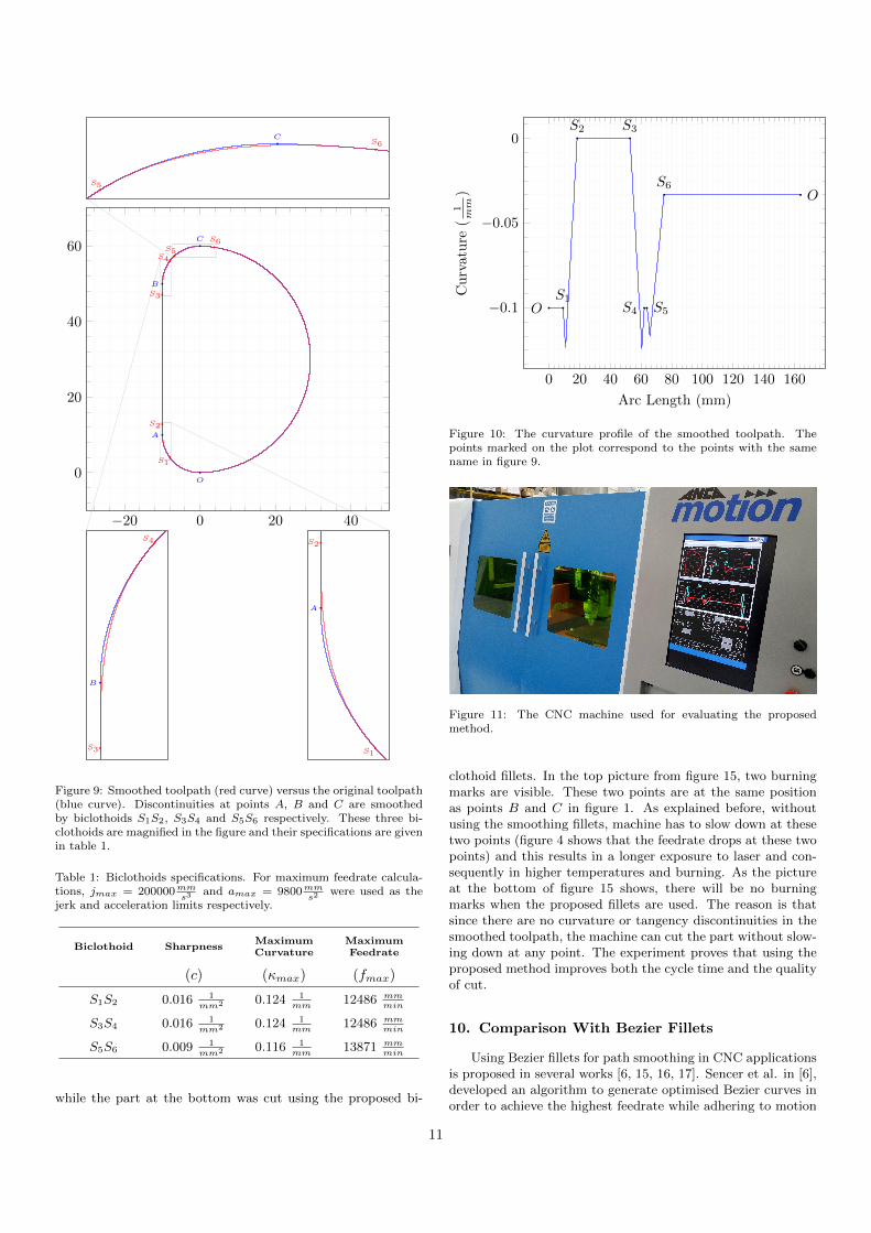
In order to assess the robustness and speed of the proposedmethod, an extensive test was carried out. For line to linecorners, angles from 0.00001 degrees to 150.00000 degrees withsteps of 0.000001 degrees were examined. Also a wide rangeof line to arc and arc to arc cases, with arc radii ranging from0.1mm to 1000mm and angles ranging from 0 to 150 degreeswere tested. Overall, more than 10 million different cases weretested and the algorithm converged in all of the tests. Six ofthese cases are portrayed in figure 8 to show some examples ofthe different cases that have been examined.
Using a computer with a dual-core CPU running at a clockrate of 2.4 GHz, the average fitting time for line to line cornerswas only 5 microseconds. For line to arc and arc to arc casesthe average fitting time was 42 microseconds. Although thefillet fitting time for arc to arc transitions is longer than thesimpler case of line to line transitions, it is still small enoughfor using in real time applications.
8
Algorithm 2: The algorithm used for finding a bi-clothoid that starts at a point on Q1, ends at a pointon Q2 and has G2-continuity with both shapes sothat the deviation between the biclothoid and thetoolpath composed of Q1 and Q2 is smaller than tol.
Input : (Q1, Q2, tol): Q1 and Q2 define the firstshape and the second shape respectively.These shapes can be either two lines, twoarcs, or an arc and a line, tol: Themaximum permissible distance betweenthe fitted biclothoid and the originaltoolpath consisted of Q1 and Q2.
Output: (c1, c2, s1, s2): The biclothoid fillet withlimited deviation from the originaltoolpath.
1 Function BiclothoidWithTolerance (Q1, Q2, tol)
2 (c1, c2, s1, s2)← Biclothoid(Q1, Q2, 0.0)3 d← distance between Q1, Q2 and the biclothoid
(c1, c2, s1, s2)4 if (d < tol) then5 return (c1, c2, s1, s2)6 end7 ε← 0.01× tol8 t1 ← 0.09 t2 ← 1.0
10 y1 ← d− tol11 y2 ← 0.012 repeat13 t3 = t1y2−t2y1
y2−y114 (c1, c2, s1, s2)← Biclothoid(Q1, Q2, t3)15 d← distance between Q1, Q2 and the
biclothoid (c1, c2, s1, s2)16 y3 ← d− tol17 if (y3 × y1 > 0) then18 y1 = y319 t1 = t320 else21 y2 = y322 t2 = t323 end
24 until (y3 < ε)25 return (c1, c2, s1, s2)
26 end
0 2 4
−1
0
1
2
(a)
0 2 4−2
−1
0
1
2
(b)
0 2 4
−1
0
1
(c)
0 2 4
−1
0
1
(d)
0 2 4
−1
0
1
(e)
0 2 4
−1
0
1
(f)
Figure 8: Examples of biclothoid fillets. In all 6 cases, the deviationbetween the original toolpath and the fillet is limited to 0.5 mm.(a) Arc to arc with acute angle (b) Arc to arc with acute angle andchange of curvature sign (c) Line to line with acute angle (d) Arc toarc with obtuse angle (e) Line to line with obtuse angle (f) Arc toline with obtuse angle.
For fitting time measurements, an ordinary desktop com-puter was used. Nevertheless, new generations of CNC con-trollers are equipped with powerful processors on par with theone that was used for the measurements. For example, Sinu-merik 840D manufactured by Siemens, takes advantage of amulti-core CPU with a clock rate up to 2.4 GHz [39]. As an-other example, the CNC controller that was used for machiningtrials reported in section 9, has a quad-core CPU with a clockfrequency of 2.3 GHz [36]. It should also be noted that thefitting algorithm needs to run only once for each discontinuity.Therefore, the computational burden of the smoothing algo-rithm will be minimal.
8. Maximum Velocity On Biclothoid Fillets
In this section, the maximum permissible velocity whenmoving on a clothoid will be calculated. It should be notedthat moving on any path which is not linear, like a circle ora clothoid, requires non-zero acceleration and jerk to be ap-plied by the axes that are participating in the move. Assumingconstant tangential velocity (path velocity), in the case of acircle, it can be proved that the maximum acceleration andjerk of each of the participating axes, can be calculated fromequations 16 and 17 respectively.
amax =v2
r= κ× v2 (16)
jmax =v3
r2= κ2 × v3 (17)
9
In these equations, v is the path velocity, κ = 1r
denotes thecurvature and amax and jmax, show the maximum accelerationand jerk that will be generated on each of the participatingaxes respectively. These equations show that even when thepath velocity (v) is fixed, the motors which are moving themachine, will have to apply potentially large acceleration andjerk values in order to move the machine on a circle. Since themaximum acceleration and jerk that a motor can generate arelimited, path velocity should be limited accordingly. Equations18 and 19 can be used to calculate the maximum velocity for afull circle.
v1 =√alim × r =
√alimκ
(18)
v2 = 3√jlim × r2 =
3
√jlimκ2
(19)
The maximum path velocity that can be applied will bemin(v1, v2) where v1 and v2 are calculated using equations 18and 19 respectively. In these equations, alim is the accelerationlimit and jlim denotes the jerk limit. In the rest of this section,similar equations will be derived for clothoids. Since a circulararc is a special case of a clothoid, the equations presented abovewill be proved in the process as well.
Starting from equation 5, the velocity of the X axis can bederived as equation 20.
vx(s) =dx(s)
dt=ds
dt× dx(s)
ds
=v × cos(θ0 + κ0s+1
2cs2) (20)
In this equation, vx(s) denotes the velocity of the X axis, vis the path velocity, and θ0, κ0, c and s have the same meaningas in equation 5.
Assuming constant tangential velocity, taking the deriva-tive of equation 20, will give the acceleration of the X axis inequation 21.
ax(s) =dvx(s)
dt=ds
dt× dvx(s)
ds
=− v2 × (cs+ κ0)× sin(θ0 + κ0s+1
2cs2) (21)
Finally taking the derivative once again, gives equation 22for the jerk of the X axis when moving on a clothoid.
jx(s) =dax(s)
dt=ds
dt× dax(s)
ds
=− v3 × c× sin(θ0 + κ0s+1
2cs2)
−v3 × (cs+ κ0)2 × cos(θ0 + κ0s+1
2cs2) (22)
Similar equations can be extracted for the Y axis. Theequation for jerk in 22 has two components. The first com-ponent (−v3 × c × sin(θ0 + κ0s + 1
2cs2)) makes a right angle
with the unit tangent vector and is known as centripetal jerk[40, 41]. It is evident that this component is directly propor-tional to the derivative of curvature (sharpness) denoted by cin the equation.
In equations 21 and 22, The maximum values for ax and jxdepend on several factors. In order to simplify the equations
and derive a limit that works in all situations, a clothoid whichcovers 360 degrees (like a full circle but with potentially vari-able radius), and its curvature varies from κ0 to κe = cs + κ0
with a maximum curvature of κmax = max(κ0, κe) can be as-sumed. Using this assumption, the maximum of the sine andcosine terms will become 1. In this case, maximum accelera-tion and jerk values can be calculated using equations 23 and24 respectively.
amax = κmax × v2 (23)
jmax =√c2 + κmax
4 × v3 (24)
Finally, the maximum path velocity that can be applied toensure that the acceleration and jerk limits are not exceededcan be calculated from equations 25 to 27.
v1 =
√alimκmax
(25)
v2 = 3
√jlim√
c2 + κmax4
(26)
v = min(v1, v2) (27)
It is evident that equations 18 and 19 are special cases ofequations 25 and 26 when c = 0 and κmax = κ. This reflectsthe fact that circular arcs are special cases of clothoids.
9. Case Study
In this section, the example given in section 3 is processedand three biclothoids are fitted to eliminate the discontinuities.The smoothed toolpath is plotted in figure 9. The introduceddeviation is very small (100 microns) and consequently it isnot easy to distinguish between the original toolpath and thesmoothed toolpath in the plot. To show the deviation, bi-clothoids and transition points are portrayed in three magni-fied boxes in figure 9. In order to better highlight how clothoidsact as transition curves between two arcs and between a lineand an arc, the curvature profile of the smoothed toolpath isalso plotted in figure 10. In figure 10, the clothoids are charac-terised by their linear curvature profiles, while the arcs can bedistinguished by their constant curvature.
Table 1 shows the data for the three fitted biclothoids.The maximum feedrate value in the table is calculated usingequations 25 to 27 assuming jmax = 200000mm
s3and amax =
9800mms2
for jerk and acceleration limits respectively. As long asthe feedrate is limited to these values, the acceleration and jerkwhen the biclothoid move is being processed, will not exceedthe limits.
The smoothed toolpath was given to an ANCA MotionAMC5 CNC controller [36] on a laser cutting machine (fig-ure 11). Figure 12 shows the path velocity. Unlike the non-smoothed case in figure 4, the machine can maintain a highfeedrate when cutting the smoothed toolpath.
Figure 13 showing the acceleration of the X and Y axesexhibits no step changes in acceleration. This is different fromfigure 2 where sudden changes in the acceleration are visible.Similarly looking at the jerk profile in 14, no jerk spikes can beseen.
Two pictures of the cut results are given in figure 15. Thepart on the top was cut without using the smoothing fillets,
10
−20 0 20 40
0
20
40
60
O
A
B
C
S1
S2
S3
S4
S5
S6
C
S5
S6
B
S3
S4
A
S1
S2
Figure 9: Smoothed toolpath (red curve) versus the original toolpath(blue curve). Discontinuities at points A, B and C are smoothedby biclothoids S1S2, S3S4 and S5S6 respectively. These three bi-clothoids are magnified in the figure and their specifications are givenin table 1.
Table 1: Biclothoids specifications. For maximum feedrate calcula-tions, jmax = 200000mm
s3and amax = 9800mm
s2were used as the
jerk and acceleration limits respectively.
Biclothoid SharpnessMaximumCurvature
MaximumFeedrate
(c) (κmax) (fmax)
S1S2 0.016 1mm2 0.124 1
mm12486 mm
min
S3S4 0.016 1mm2 0.124 1
mm12486 mm
min
S5S6 0.009 1mm2 0.116 1
mm13871 mm
min
while the part at the bottom was cut using the proposed bi-
0 20 40 60 80 100 120 140 160
−0.1
−0.05
0
OS1
S2 S3
S4 S5
S6O
Arc Length (mm)
Cu
rvat
ure
(1mm
)
Figure 10: The curvature profile of the smoothed toolpath. Thepoints marked on the plot correspond to the points with the samename in figure 9.
Figure 11: The CNC machine used for evaluating the proposedmethod.
clothoid fillets. In the top picture from figure 15, two burningmarks are visible. These two points are at the same positionas points B and C in figure 1. As explained before, withoutusing the smoothing fillets, machine has to slow down at thesetwo points (figure 4 shows that the feedrate drops at these twopoints) and this results in a longer exposure to laser and con-sequently in higher temperatures and burning. As the pictureat the bottom of figure 15 shows, there will be no burningmarks when the proposed fillets are used. The reason is thatsince there are no curvature or tangency discontinuities in thesmoothed toolpath, the machine can cut the part without slow-ing down at any point. The experiment proves that using theproposed method improves both the cycle time and the qualityof cut.
10. Comparison With Bezier Fillets
Using Bezier fillets for path smoothing in CNC applicationsis proposed in several works [6, 15, 16, 17]. Sencer et al. in [6],developed an algorithm to generate optimised Bezier curves inorder to achieve the highest feedrate while adhering to motion
11
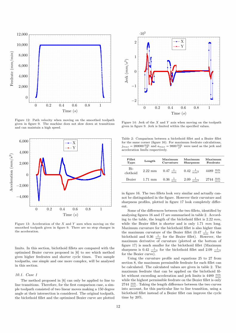
0 0.2 0.4 0.6 0.8 1
0
2,000
4,000
6,000
8,000
10,000
12,000
Time (s)
Fee
dra
te(mm/min
)
Figure 12: Path velocity when moving on the smoothed toolpathgiven in figure 9. The machine does not slow down at transitionsand can maintain a high speed.
0 0.2 0.4 0.6 0.8 1
−4,000
−2,000
0
2,000
4,000
6,000
Time (s)
Acc
eler
atio
n(mm/s
2)
XY
Figure 13: Acceleration of the X and Y axes when moving on thesmoothed toolpath given in figure 9. There are no step changes inthe acceleration.
limits. In this section, biclothoid fillets are compared with theoptimised Bezier curves proposed in [6] to see which methodgives higher feedrates and shorter cycle times. Two sampletoolpaths, one simple and one more complex, will be analysedin this section.
10.1. Case 1
The method proposed in [6] can only be applied to line toline transitions. Therefore, for the first comparison case, a sim-ple toolpath consisted of two linear moves making a 150 degreeangle at their intersection is considered. The original toolpath,the biclothoid fillet and the optimised Bezier curve are plotted
0 0.2 0.4 0.6 0.8 1
−2
−1
0
1
2
·105
Time (s)
Jer
k(mm/s3
)
XY
Figure 14: Jerk of the X and Y axis when moving on the toolpathgiven in figure 9. Jerk is limited within the specified values.
Table 2: Comparison between a biclothoid fillet and a Bezier filletfor the same corner (figure 16). For maximum feedrate calculations,jmax = 200000mm
s3and amax = 9800mm
s2were used as the jerk and
acceleration limits respectively.
FilletType
LengthMaximumCurvature
MaximumSharpness
MaximumFeedrate
Bi-clothoid
2.22 mm 0.47 1mm
0.42 1mm2 4489 mm
min
Bezier 1.71 mm 0.36 1mm
2.09 1mm2 2744 mm
min
in figure 16. The two fillets look very similar and actually can-not be distinguished in the figure. However their curvature andsharpness profiles, plotted in figure 17 look completely differ-ent.
Some of the differences between the two fillets, identified byanalysing figures 16 and 17 are summarised in table 2. Accord-ing to the table, the length of the biclothoid fillet is 2.22 mm,while the Bezier fillet is shorter and is only 1.71 mm long.Maximum curvature for the biclothoid fillet is also higher thanthe maximum curvature of the Bezier fillet (0.47 1
mmfor the
biclothoid and 0.36 1mm
for the Bezier fillet). However, themaximum derivative of curvature (plotted at the bottom offigure 17) is much smaller for the biclothoid fillet (Maximumsharpness is 0.42 1
mm2 for the biclothoid fillet and 2.09 1mm2
for the Bezier curve).Using the curvature profile and equations 25 to 27 from
section 8, the maximum permissible feedrate for each fillet canbe calculated. The calculated values are given in table 2. Themaximum feedrate that can be applied on the biclothoid fil-let without exceeding acceleration and jerk limits is 4489 mm
min
while the highest permissible feedrate on the Bezier fillet is only2744 mm
min. Taking the length difference between the two curves
into account, for this particular line to line transition, using abiclothoid fillet instead of a Bezier fillet can improve the cycletime by 20%.
12
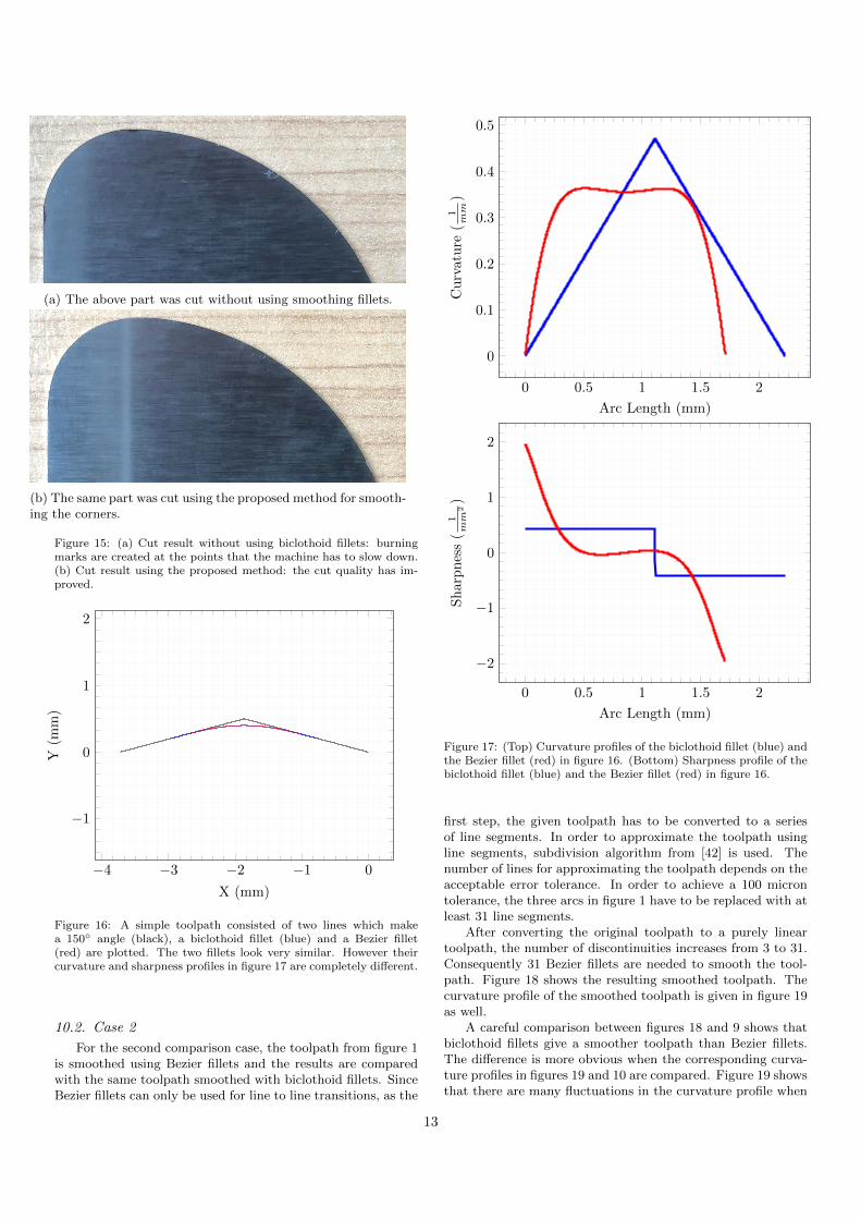
(a) The above part was cut without using smoothing fillets.
(b) The same part was cut using the proposed method for smooth-ing the corners.
Figure 15: (a) Cut result without using biclothoid fillets: burningmarks are created at the points that the machine has to slow down.(b) Cut result using the proposed method: the cut quality has im-proved.
−4 −3 −2 −1 0
−1
0
1
2
X (mm)
Y(m
m)
Figure 16: A simple toolpath consisted of two lines which makea 150 angle (black), a biclothoid fillet (blue) and a Bezier fillet(red) are plotted. The two fillets look very similar. However theircurvature and sharpness profiles in figure 17 are completely different.
10.2. Case 2
For the second comparison case, the toolpath from figure 1is smoothed using Bezier fillets and the results are comparedwith the same toolpath smoothed with biclothoid fillets. SinceBezier fillets can only be used for line to line transitions, as the
0 0.5 1 1.5 2
0
0.1
0.2
0.3
0.4
0.5
Arc Length (mm)
Cu
rvat
ure
(1mm
)
0 0.5 1 1.5 2
−2
−1
0
1
2
Arc Length (mm)
Sh
arp
nes
s(
1mm
2)
Figure 17: (Top) Curvature profiles of the biclothoid fillet (blue) andthe Bezier fillet (red) in figure 16. (Bottom) Sharpness profile of thebiclothoid fillet (blue) and the Bezier fillet (red) in figure 16.
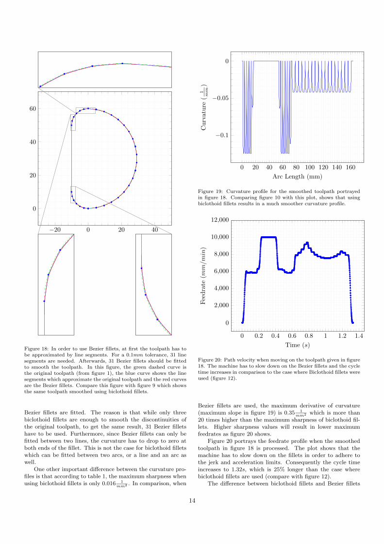
first step, the given toolpath has to be converted to a seriesof line segments. In order to approximate the toolpath usingline segments, subdivision algorithm from [42] is used. Thenumber of lines for approximating the toolpath depends on theacceptable error tolerance. In order to achieve a 100 microntolerance, the three arcs in figure 1 have to be replaced with atleast 31 line segments.
After converting the original toolpath to a purely lineartoolpath, the number of discontinuities increases from 3 to 31.Consequently 31 Bezier fillets are needed to smooth the tool-path. Figure 18 shows the resulting smoothed toolpath. Thecurvature profile of the smoothed toolpath is given in figure 19as well.
A careful comparison between figures 18 and 9 shows thatbiclothoid fillets give a smoother toolpath than Bezier fillets.The difference is more obvious when the corresponding curva-ture profiles in figures 19 and 10 are compared. Figure 19 showsthat there are many fluctuations in the curvature profile when
13
−20 0 20 40
0
20
40
60
Figure 18: In order to use Bezier fillets, at first the toolpath has tobe approximated by line segments. For a 0.1mm tolerance, 31 linesegments are needed. Afterwards, 31 Bezier fillets should be fittedto smooth the toolpath. In this figure, the green dashed curve isthe original toolpath (from figure 1), the blue curve shows the linesegments which approximate the original toolpath and the red curvesare the Bezier fillets. Compare this figure with figure 9 which showsthe same toolpath smoothed using biclothoid fillets.
Bezier fillets are fitted. The reason is that while only threebiclothoid fillets are enough to smooth the discontinuities ofthe original toolpath, to get the same result, 31 Bezier filletshave to be used. Furthermore, since Bezier fillets can only befitted between two lines, the curvature has to drop to zero atboth ends of the fillet. This is not the case for biclothoid filletswhich can be fitted between two arcs, or a line and an arc aswell.
One other important difference between the curvature pro-files is that according to table 1, the maximum sharpness whenusing biclothoid fillets is only 0.016 1
mm2 . In comparison, when
0 20 40 60 80 100 120 140 160
−0.1
−0.05
0
Arc Length (mm)
Cu
rvat
ure
(1mm
)
Figure 19: Curvature profile for the smoothed toolpath portrayedin figure 18. Comparing figure 10 with this plot, shows that usingbiclothoid fillets results in a much smoother curvature profile.
0 0.2 0.4 0.6 0.8 1 1.2 1.4
0
2,000
4,000
6,000
8,000
10,000
12,000
Time (s)
Fee
dra
te(mm/m
in)
Figure 20: Path velocity when moving on the toolpath given in figure18. The machine has to slow down on the Bezier fillets and the cycletime increases in comparison to the case where Biclothoid fillets wereused (figure 12).
Bezier fillets are used, the maximum derivative of curvature(maximum slope in figure 19) is 0.35 1
mm2 which is more than20 times higher than the maximum sharpness of biclothoid fil-lets. Higher sharpness values will result in lower maximumfeedrates as figure 20 shows.
Figure 20 portrays the feedrate profile when the smoothedtoolpath in figure 18 is processed. The plot shows that themachine has to slow down on the fillets in order to adhere tothe jerk and acceleration limits. Consequently the cycle timeincreases to 1.32s, which is 25% longer than the case wherebiclothoid fillets are used (compare with figure 12).
The difference between biclothoid fillets and Bezier fillets
14
Table 3: Comparison between biclothoid fillets and Bezier fillets forsmoothing the toolpath from figure 1 with two different tolerancevalues. When the tolerance gets tighter, a larger number of Bezierfillets have to be used and the cycle time increases significantly. Bi-clothoid fillets on the contrary, show a good performance at smallertolerance values.
Fillet type ToleranceNumber of
filletsCycle time
Biclothoid 0.1mm 3 1.048s
Biclothoid 0.01mm 3 1.053s
Bezier 0.1mm 31 1.322s
Bezier 0.01mm 96 1.723s
becomes more prominent at tighter tolerance settings. Table3 compares Bezier and biclothoid fillets when used to smooththe toolpath from figure 1 at two different tolerance settings.When the tolerance is set to 10 microns, 96 Bezier fillets willbe needed and the cycle time increases to 1.72s. For achievingthe same tolerance, only three biclothoid fillets will suffice andthe cycle time will drop to 1.05s. In this scenario, the cycletime that Bezier fillets give is 63% longer than the case wherebiclothoid fillets are used.
11. Conclusion and Future Work
A method for smoothing corners using biclothoid fillets waspresented. The proposed method can be used to smooth outdiscontinuities in curvature and in tangency for line to line, lineto arc, and arc to arc transitions. To the authors’ knowledgethis is the first method that can be applied to arc to arc andline to arc corners in addition to line to line transitions.
For smoothing line to line transitions, analytical solutionshave been developed. However for transitions between two arcsor a line and arc, specially if arc length parameterisation is ofimportance, iterative algorithms have to be used. To evaluatethe robustness of the proposed method, the performance of thedeveloped algorithms was extensively tested and the resultswere reported.
A comparison with Bezier fillets shows that using the pro-posed method can result in a significantly shorter cycle timewith a much smaller number of fillets. It was demonstratedthat since Bezier fillets can only be fitted between two lines,the toolpath has to be broken into a large number of lines andconsequently a large number of fillets have to be fitted. Theproposed method does not have this limitation.
The proposed method has a number of important advan-tages and satisfies all of the requirements explained in section3:
a. G2-continuity: The generated toolpath is curvaturecontinuous and eliminates any discontinuities in the orig-inal toolpath.
b. Bounded maximum error: the deviation between thesmoothed toolpath and the original toolpath can be lim-ited to a specified tolerance to maintain the accuracy ofthe manufactured parts.
c. Analytical arc length formula: the arc length of thegenerated fillets is readily available and unlike Bezier
curves, Quintic splines, etc. there is no need to use inte-gration to calculate the arc length.
d. Arc length parameterisation: the generated path is arclength parameterised which makes it easier to interpo-late. There will be no feedrate fluctuations when inter-polating the path and unlike PH curves, special interpo-lators are not required.
e. Minimum curvature change: biclothoid fillets have atriangle shaped curvature profile which gives the smallestsharpness for a specified arc length [3].
To demonstrate the effectiveness of the proposed method aCNC controller equipped with a jerk limited interpolator wasused. It was verified that without modifying the toolpath, thecontroller has to slow down the machine at line to arc and arcto arc transitions to keep the jerk within the limits. Usingthe proposed method, the controller is able to maintain a highfeedrate without introducing any jerk spikes. For calculatingthe feedrate limit not only the curvature but also the derivativeof curvature were taken into account.
The proposed method can be extended to achieve higherdegrees of continuity like G3-continuity, provided that the CNCcontroller can generate a jounce limited velocity profile. ForG3-continuity, instead of clothoids, cubic spirals [43] may haveto be used. Future work could also investigate using clothoidsfor generating smooth toolpaths for 5 axis CNC applications.
Acknowledgment
The authors would like to thank ANCA Motion Pty. Ltd.for providing the equipment and machinery to evaluate the pro-posed method.
[1] S.-H. Suh, Theory and design of CNC systems, Springer, 2008.[2] A. Scheuer, T. Fraichard, Planning continuous-curvature paths
for car-like robots, in: Proceedings of the 1996 IEEE/RSJ In-ternational Conference on Intelligent Robots and Systems ’96,IROS 96, Vol. 3, 1996, pp. 1304–1311. doi:10.1109/IROS.1996.568985.
[3] W. Nelson, Continuous-curvature paths for autonomous vehi-cles, Proceedings, 1989 International Conference on Roboticsand Automation (1989) 1260–1264doi:10.1109/ROBOT.1989.100153.
[4] D. H. Shin, S. Singh, Path Generation for Robot Vehicles UsingComposite Clothoid Segments, Tech. Rep. CMU-RI-TR-90-31,Robotics Institute, Pittsburgh, PA (Dec. 1990).
[5] M. Brezak, I. Petrovic, Path smooth Using Clothoids for Dif-ferential Drive Mobile Robots, in: 18th IFAC World Congress2011, 2011.
[6] B. Sencer, K. Ishizaki, E. Shamoto, A curvature optimal sharpcorner smooth algorithm for high-speed feed motion generationof NC systems along linear tool paths, International Journalof Advanced Manufacturing Technology 76 (9-12) (2014) 1977–1992. doi:10.1007/s00170-014-6386-2.
[7] A. Shahzadeh, A. Khosravi, S. Nahavandi, Path planning forcnc machines considering centripetal acceleration and jerk, in:2013 IEEE International Conference on Systems, Man, and Cy-bernetics, 2013, pp. 1759–1764. doi:10.1109/SMC.2013.303.
[8] K. Erkorkmaz, Y. Altintas, High speed CNC system design.Part I: Jerk limited trajectory generation and quintic spline in-terpolation, International Journal of Machine Tools and Manu-facture 41 (9) (2001) 1323–1345. doi:10.1016/S0890-6955(01)00002-5.
[9] A. Yuen, K. Zhang, Y. Altintas, Smooth trajectory genera-tion for five-axis machine tools, International Journal of Ma-chine Tools and Manufacture 71 (2013) 11–19. doi:10.1016/j.ijmachtools.2013.04.002.
15
[10] K. Erkorkmaz, C. H. Yeung, Y. Altintas, Virtual CNC system.Part II. High speed contouring application, International Jour-nal of Machine Tools and Manufacture 46 (10) (2006) 1124–1138. doi:10.1016/j.ijmachtools.2005.08.001.
[11] F. C. Wang, D. C. H. Yang, Nearly arc-length parame-terized quintic-spline interpolation for precision machining,Computer-Aided Design 25 (5) (1993) 281–288. doi:10.1016/
0010-4485(93)90085-3.[12] K. Erkorkmaz, Y. Altintas, Quintic Spline Interpolation With
Minimal Feed Fluctuation (2005). doi:10.1115/1.1830493.[13] S. Yutkowitz, Apparatus and method for smooth cornering in a
motion control system, US Patent 6,922,606 (Jul. 26 2005).[14] X. Beudaert, P. Y. Pechard, C. Tournier, 5-Axis Tool Path
Smoothing Based on Drive Constraints, International Journalof Machine Tools and Manufacture 51 (12) (2011) 958–965.doi:10.1016/j.ijmachtools.2011.08.014.
[15] K. Yang, S. Sukkarieh, An Analytical Continuous-CurvaturePath-smoothing Algorithm, IEEE Transactions on Robotics26 (3) (2010) 561–568. doi:10.1109/TRO.2010.2042990.
[16] Q. Bi, Y. Wang, L. Zhu, H. Ding, A Practical Continuous-Curvature Bezier Transition Algorithm for High-Speed Ma-chining of Linear Tool Path, Intelligent Robotics and Appli-cations: 4th International Conference, ICIRA 2011, Aachen,Germany, December 6-8, 2011, Proceedings, Part II (2011) 465–476doi:10.1007/978-3-642-25489-5_45.URL http://dx.doi.org/10.1007/978-3-642-25489-5_45
[17] Q. Bi, J. Shi, Y. Wang, L. Zhu, H. Ding, Analytical curvature-continuous dual-Bezier corner transition for five-axis linear toolpath, International Journal of Machine Tools and Manufacture91 (2015) 96–108. doi:10.1016/j.ijmachtools.2015.02.002.
[18] D. J. Walton, D. S. Meek, G2 blends of linear segments withcubics and Pythagorean-hodograph quintics, InternationalJournal of Computer Mathematics 86 (9) (2009) 1498–1511.doi:10.1080/00207160701828157.URL http://www.tandfonline.com/doi/abs/10.1080/
00207160701828157
[19] W. Fan, C.-H. Lee, J.-H. Chen, A realtime curvature-smooth in-terpolation scheme and motion planning for CNC machining ofshort line segments, International Journal of Machine Tools andManufacture 96 (2015) 27–46. doi:10.1016/j.ijmachtools.
2015.04.009.[20] H. Zhao, L. Zhu, H. Ding, A real-time look-ahead interpolation
methodology with curvature-continuous B-spline transitionscheme for CNC machining of short line segments, InternationalJournal of Machine Tools and Manufacture 65 (5-8) (2013)88–98. doi:10.1016/j.ijmachtools.2012.10.005.URL https://doi.org/10.1016/j.ijmachtools.
2012.10.005http://link.springer.com/10.1007/
s00170-015-7776-9http://linkinghub.elsevier.com/
retrieve/pii/S0890695512001885
[21] X. Beudaert, S. Lavernhe, C. Tournier, 5-Axis Local CornerRounding of Linear Tool Path Discontinuities, InternationalJournal of Machine Tools and Manufacture 73 (2013) 9–16.doi:10.1016/j.ijmachtools.2013.05.008.
[22] S. Tulsyan, Y. Altintas, Local toolpath smoothing for five-axismachine tools, International Journal of Machine Tools and Man-ufacture 96 (2015) 15–26. doi:10.1016/j.ijmachtools.2015.
04.014.[23] J. Yang, A. Yuen, An analytical local corner smoothing al-
gorithm for five-axis CNC machining, International Journalof Machine Tools and Manufacture 123 (July) (2017) 22–35.doi:10.1016/j.ijmachtools.2017.07.007.
[24] J. Shi, Q. Z. Bi, L. M. Zhu, Y. H. Wang, Corner rounding oflinear five-axis tool path by dual PH curves blending, Inter-national Journal of Machine Tools and Manufacture 88 (2015)223–236. doi:10.1016/j.ijmachtools.2014.09.007.
[25] S. Tajima, B. Sencer, Kinematic corner smoothing forhigh speed machine tools, International Journal of MachineTools and Manufacture 108 (2016) 27–43. doi:10.1016/j.
ijmachtools.2016.05.009.[26] S. Tajima, B. Sencer, Global tool-path smoothing for CNC ma-
chine tools with uninterrupted acceleration, International Jour-nal of Machine Tools and Manufacture 121 (November 2016)(2017) 81–95. doi:10.1016/j.ijmachtools.2017.03.002.
[27] M. a. Heald, Rational Approximations for the Fresnel Integrals,Mathematics of Computation 44 (170) (1985) 459. doi:10.
2307/2007965.[28] M. Brezak, I. Petrovic, Real-time approximation of clothoids
with bounded error for path planning applications, IEEE Trans-actions on Robotics 30 (2) (2014) 507–515. doi:10.1109/TRO.
2013.2283928.[29] H. Zhao, L. Zhu, H. Ding, A parametric interpolator with min-
imal feed fluctuation for CNC machine tools using arc-lengthcompensation and feedback correction, International Journal ofMachine Tools and Manufacture 75 (2013) 1–8. doi:10.1016/
j.ijmachtools.2013.08.002.[30] Y. Sun, Y. Zhao, Y. Bao, D. Guo, A smooth curve evolution
approach to the feedrate planning on five-axis toolpath withgeometric and kinematic constraints, International Journal ofMachine Tools and Manufacture 97 (2015) 86–97. doi:10.1016/j.ijmachtools.2015.07.002.
[31] M. Chen, W. S. Zhao, X. C. Xi, Augmented Taylor’s expan-sion method for B-spline curve interpolation for CNC machinetools, International Journal of Machine Tools and Manufacture94 (2015) 109–119. doi:10.1016/j.ijmachtools.2015.04.013.
[32] M. Heng, K. Erkorkmaz, Design of a nurbs interpolator withminimal feed fluctuation and continuous feed modulation ca-pability, International Journal of Machine Tools and Manufac-ture 50 (3) (2010) 281 – 293. doi:https://doi.org/10.1016/
j.ijmachtools.2009.11.005.[33] R. T. Farouki, S. Shah, Real-time CNC interpolators for
Pythagorean-hodograph curves, Computer Aided GeometricDesign 13 (7) (1996) 583–600. doi:10.1016/0167-8396(95)
00047-X.[34] R. Farouki, J. Manjunathaiah, D. Nicholas, G.-F. Yuan,
S. Jee, Variable-feedrate CNC interpolators for constant ma-terial removal rates along Pythagorean-hodograph curves,Computer-Aided Design 30 (8) (1998) 631–640. doi:10.1016/
S0010-4485(98)00020-7.[35] T. R. Kramer, F. M. Proctor, E. Messina, The NIST
RS274/NGC Interpreter-Version 3, National Institute of Stan-dards and Technology (NIST), NISTIR 6556.
[36] AMC5 CNC by ANCA Motion, https://www.ancamotion.com/cnc/amc5, accessed: 2017-10-07.
[37] J. Jahanpour, M.-C. Tsai, M.-Y. Cheng, I.-H. Liu, Contour Fol-lowing Using C2 PH Quintic Spline Curve Interpolators, IFACProceedings Volumes 44 (1) (2011) 9361 – 9366, 18th IFACWorld Congress.
[38] A. A. Taha, A. Hanbury, An efficient algorithm for calculat-ing the exact Hausdorff distance, IEEE transactions on patternanalysis and machine intelligence 37 (11) (2015) 2153–2163.
[39] Catalog NC 62: SINUMERIK 840 Equipment for Machine Tools(2016).
[40] W. L. Nelson, Continuous steering-function control of robotcarts, IEEE Transactions on Industrial Electronics 36 (3) (1989)330–337. doi:10.1109/41.31495.
[41] A. C. Lee, M. T. Lin, Y. R. Pan, W. Y. Lin, The feedratescheduling of NURBS interpolator for CNC machine tools, CADComputer Aided Design 43 (6) (2011) 612–628. arXiv:ISSN:
00104485, doi:10.1016/j.cad.2011.02.014.[42] D. Walton, D. Meek, Approximation of quadratic bzier curves
by arc splines, Journal of Computational and Applied Mathe-matics 54 (1) (1994) 107 – 120. doi:https://doi.org/10.1016/0377-0427(94)90398-0.URL http://www.sciencedirect.com/science/article/pii/
0377042794903980
[43] Y. Kanayama, B. I. Hartman, Smooth local path planning forautonomous vehicles, in: Proceedings, 1989 International Con-ference on Robotics and Automation, 1989, pp. 1265–1270 vol.3.doi:10.1109/ROBOT.1989.100154.
16