Smoothed dissipative particle dynamics model for polymer molecules in suspension

Sergey Litvinov,1 Marco Ellero,1,2 Xiangyu Hu,1 and Nikolaus A. Adams1

1Lehrstuhl für Aerodynamik, Technische Universität München, 85747 Garching, Germany2Departamento de Física Fundamental, UNED, Apartado 60141, 28080 Madrid, Spain

�Received 4 October 2007; published 5 June 2008�

We present a model for a polymer molecule in solution based on smoothed dissipative particle dynamics�SDPD� �Español and Revenga, Phys. Rev. E 67, 026705 �2003��. This method is a thermodynamicallyconsistent version of smoothed particle hydrodynamics able to discretize the Navier-Stokes equations and, atthe same time, to incorporate thermal fluctuations according to the fluctuation-dissipation theorem. Within theframework of the method developed for mesoscopic multiphase flows by Hu and Adams �J. Comput. Phys.213, 844 �2006��, we introduce additional finitely extendable nonlinear elastic interactions between particlesthat represent the beads of a polymer chain. In order to assess the accuracy of the technique, we analyze thestatic and dynamic conformational properties of the modeled polymer molecule in solution. Extensive tests ofthe method for the two-dimensional �2D� case are performed, showing good agreement with the analyticaltheory. Finally, the effect of confinement on the conformational properties of the polymer molecule is inves-tigated by considering a 2D microchannel with gap H varying between 1 and 10 �m, of the same order as thepolymer gyration radius. Several SDPD simulations are performed for different chain lengths corresponding toN=20–100 beads, giving a universal behavior of the gyration radius RG and polymer stretch X as functions ofthe channel gap when normalized properly.

DOI: 10.1103/PhysRevE.77.066703 PACS number�s�: 47.11.St, 05.10.�a, 47.57.Ng

I. INTRODUCTION

The increasing technological need to create and manipu-late structures on micrometer scales and smaller for the de-sign of micro- and nanodevices has triggered the develop-ment of many numerical methods for simulating problems atmesoscales �1–3�. One specific area of investigation is mi-crofluidics, which refers to the fluid dynamics occurring indevices or flow configurations with the smallest designlength on the order of micrometers �4�. A typical applicationis, for example, the dynamics of a polymer molecule in achannel or other confined geometries such as micropumps,mixers, and sensors. For instance, the mechanical responseof a tethered DNA molecule to hydrodynamic flow is cur-rently under investigation by some groups and can be usedfor local sensing, leading to the concept of using an immo-bilized DNA molecule as a mechanical-fluidic sensor or formicrofabricated metallic wires and networks �5–7�. The de-velopment of single-molecule concepts is of great impor-tance for future applications in proteomics, genomics, andbiomedical diagnostics, and it is therefore evident that theability to improve the predictive computational tools at thisspatiotemporal level would greatly improve the engineeringtasks.

It is worth noting that the Navier-Stokes equations de-scribing the dynamics of a Newtonian liquid at the macro-scopic level still remain valid at the microfluidic scales,therefore providing a natural framework based on the con-tinuum description. On the other hand, it is also clear that,whenever the physical dimensions of the considered objects�i.e., polymer molecules, colloidal particles� are in the sub-micrometer range, the surrounding fluid starts to be affectedby the presence of its underlying molecular structure, andhydrodynamic variables will be influenced by thermody-namic fluctuations according to the Landau and Lifshitz

theory �8�. Standard macroscopic approaches, based, for ex-ample, on finite-volume or finite-element methods, are notsuitable for this type of simulation. They neglect thermalfluctuations which, as mentioned above, are the most crucialingredient of the mesoscopic dynamics. On the other hand,direct microscopic approaches, such as molecular dynamics,are able to resolve the smallest details of the molecular struc-tures but they are computationally very expensive and arelimited by the available computer resources. Nowadays,these approaches are restricted to computational domains oflength of the order of nanometers which represent only thesmallest scales �dimensions of one nanostructure� in therange covered by the considered system. Despite their highcomputational cost, molecular dynamics �MD� methods havebeen used frequently for studying the dynamics of polymermolecules in a solvent, described by Lennard-Jones interac-tion potentials, producing valuable results �9–11�. The ad-vantage of these methods is that hydrodynamics emergesnaturally from intermolecular interactions and does not needto be modeled.

Other methods based on Brownian dynamics techniqueshave been shown recently to produce accurate results forDNA dynamics in microfluidic devices �12� but require acomplicated modeling of hydrodynamic interactions �in par-ticular when coupled with the no-slip boundary conditions atthe walls� mediated by a modified Rotne-Prager-Yamakawatensor. To remedy these problems, various researchers havefocused in the past on mesoscopic methods which employnumerically effective coarse-grained models retaining therelevant hydrodynamics modes. Examples are multiparticlecollision dynamics �13�, lattice Boltzmann methods �LBMs��14�, and dissipative particle dynamics �DPD�. In particular,DPD is a mesoscopic methodology which has attracted in-creasing attention in recent years. DPD was originally pro-posed by Hoogerbrugge and Koelman in 1992 �15� and suc-cessively modified by Español and Warren in order to satisfy

PHYSICAL REVIEW E 77, 066703 �2008�

1539-3755/2008/77�6�/066703�12� ©2008 The American Physical Society066703-1

thermodynamic consistency �16�. The method has beenshown to capture the relevant thermodynamic and hydrody-namic effects occurring in mesoscopic systems �17–20�, andit has been applied in recent years to a wide range of physicalsituations �21–23�. Despite its great success, a number ofconceptual shortcomings have been recently pointed outwhich affect the performance and accuracy of the technique.In particular, they concern �i� the nonarbitrary choice of thefluid equation of state, �ii� no direct connection to the trans-port coefficients, �iii� the unclear definition of the physicalparticle scales, and �iv� particle penetration due to the em-ployed soft two-body potentials �24�. These drawbacks pre-vent also an a priori control of the spatiotemporal scale inDPD and require a tuning of model parameters in order tocompare the numerical results with experimental data. Allthese problems can be avoided by resorting to a further im-proved DPD version, smoothed dissipative particle dynamics�SDPD� �25�.

SDPD represents a powerful generalization of the so-called smoothed particle hydrodynamics �SPH� method�26–28� for mesoscales. Being based on a second-order dis-cretization of the Navier-Stokes �NS� equations, transport co-efficients are input parameters and do not need to be mea-sured by Green-Kubo relations as in MD or extracted viakinetic theory as in conventional DPD. In SDPD, the par-ticles represent therefore physical fluid elements whose spe-cific size determines the level of thermal fluctuations in thehydrodynamic variables. At the same time, since the methodis based on a Lagrangian discretization of the NS equations,hydrodynamic behavior is obtained at the particle scale andno coarse-graining assumption is needed.

In this paper, we propose a SDPD model for the investi-gation of the static and dynamic behavior of a polymer mol-ecule in unbounded and confined geometries. The polymermolecule is represented by a polymer chain constituted bybeads interacting by finitely extendable nonlinear elastic�FENE� forces. In order to validate the model, the two-dimensional �2D� case of a polymer molecule in a bulk sol-vent fluid is considered first. Note that 2D polymer dynamicsdoes not represent an oversimplified picture of reality, butrather reflects realistic situations often encountered in poly-mer technology, and has recently been the focus of severalnumerical and experimental investigations �29–34�. In manycases polymer dynamics occurs within a very thin layer withthickness considerably smaller than the gyration radius, andthe motion can be considered as truly two dimensional. Prac-tical examples are thin polymer films, polymers adsorbed tosurfaces, or polymers confined between biological interfaces.For example, recently Maier and Rädler performed experi-ments with a single DNA molecule electrostatically confinedto a surface of fluid lipid membranes �30�. The confinementwas found not to inhibit the lateral mobility of the molecule,and results for the conformational statistics were in goodagreement with theoretical predictions in 2D. From a nu-merical point of view, extensive Monte Carlo and moleculardynamics simulations have been performed in the past andhave proven to be extremely useful in corroborating analyti-cal theories or explaining anomalous scaling behavior inbulk and confined situations �9,11,32,35�.

In this work, static and dynamic scaling exponents areextracted from the SDPD simulations showing excellent

agreement with the theoretical Zimm predictions and previ-ous numerical results. As a further validation test, the case ofa polymer molecule confined between two parallel walls isconsidered, that is, an infinite 2D microchannel. The influ-ence that the channel gap H has on the polymer conforma-tional properties is investigated. According to previous stud-ies in the 3D case �12,20,36�, it is found that, for lengths ofthe gap comparable to the molecule gyration radius �i.e., onthe order of micrometers�, strong anisotropic effects start toaffect the polymer statistics, such as, e.g., the average gyra-tion radius and polymer stretch. In addition, the power lawbehavior of the polymer stretch as function of the normalizedchannel width has also been verified numerically, giving anexponent in excellent agreement with the analytical resultspredicted from scaling arguments in 2D by de Gennes �37�.The results will be discussed in the final section.

II. THE SIMULATION METHOD

A. Macroscopic hydrodynamics

We consider the isothermal Navier-Stokes equations on amoving Lagrangian grid

d�

dt= − � � · v , �1�

dv

dt= g −

1

�� p + F , �2�

where �, v, and g are the material density, velocity, and bodyforce, respectively. A simple equation of state is p=−�TVwhere �T is the isothermal compressibility. It can be rewrit-ten as

p = a2� . �3�

When Eqs. �1� and �2� are used for modeling of low-Reynolds-number incompressible flows with the artificial-compressibility method, a is equal to the artificial speed ofsound. An alternative equation of state for incompressibleflows is

p = p0� �

�0��

+ b , �4�

where p0, �0, �, and a are parameters. The parameters in Eq.�3� and �4� may be chosen based on a scale analysis�26,38,39� so that the density variation is less than a givenvalue. F denotes the viscous force

F =1

�� · ���� �5�

where the shear stress is ����=���v+�vT�. If the bulk vis-cosity is assumed as =0, for incompressible flow the vis-cous force simplifies to

F = ��2v , �6�

where �=� /� is the kinematic viscosity.

LITVINOV et al. PHYSICAL REVIEW E 77, 066703 �2008�

066703-2

1. Density evolution equation

Let us introduce the particle number density di, which isdefined by

di = �j

Wij , �7�

where Wij =W�rij ,h�=W��ri−r j� ,h�, and W�r ,h� is a genericshape function with compact support h which is radiallysymmetric and has the properties W�r−r��dr�=1 andlimh→0W�r−r� ,h�=�r−r�� �in this work, a quintic splinefunction has been used�. According to �7�, di will have largervalues in a dense particle region than in a dilute particleregion. Equation �7� introduces also a straightforward defini-tion of the volume of particle i, which is Vi=1 /di. The aver-age mass density of a particle is therefore defined as �i=mi /Vi where mi is the mass of a particle. Other forms ofevaluating the mass density are possible in SPH, which takeinto account a direct discretization of the continuity equationin �1�. However, the direct particle summation adopted hereand based on Eq. �7� has the advantage that the total mass isalgebraically conserved.

2. Momentum equation

Concerning the momentum equation, it has been shown�25,40� that a possible SPH discretization of the pressureforce appearing in �2� is

dvi�p�

dt= −

1

mi�

j� pi

di2 +

pj

dj2� �W

�rijeij , �8�

where dvi�p� /dt is the particle acceleration caused by pressure

effects, pi is the pressure associated with particle i �41�, andeij is the unit vector connecting particles i and j. It can beshown that this expression represents a second-order SPHdiscretization of the gradient of the scalar field p. Since thisexpression has an antisymmetric form with respect to ex-change of i and j, global conservation of momentum is sat-isfied. Equation �8� is similar to the form preferred by Mon-aghan �26�.

Concerning the viscous force, similarly to Flekkøy et al.�42�, the interparticle-averaged shear stress is approximatedas

�ij�v� =

�

rij�eijvij + vijeij� �9�

where vij =vi−v j. Hence, the particle acceleration due to theshear force in conservative form is given by

dvi�v�

dt=

�

mi�

j� 1

di2 +

1

dj2� 1

rij

�W

�rij�eij · vijeij + vij� . �10�

Note that this expression does not strictly conserve angularmomentum. Conservation of total angular momentum can berestored by adopting either suitable artificial viscosity mod-els based on interparticle central forces �26� for which,though, there is no direct connection to the Navier-Stokesform of the stress tensor, or linearly consistent versions ofSPH �43�.

B. Mesoscopic hydrodynamics

The method outlined above is strictly analogous to theSPH technique widely used to describe macroscopic flowproblems in a Lagrangian framework. In order to includemesoscopic effects, i.e., the presence of thermal fluctuationsin the physical quantities, we follow the approach given byEspañol and Revenga, i.e., smoothed dissipative particle dy-namics �25�, which represents a powerful and elegant gener-alization of SPH at the mesoscopic scales. It should be no-ticed, that the method has been generalized for the study ofviscoelastic liquids �44� and also, more recently, for mesos-copic multiphase flow problems �40�.

Thermal fluctuations

In the current SPH method the irreversible part of theparticle dynamics is

miirr = 0,

Piirr = ��j� 1

di2 +

1

dj2� 1

rij

�W

�rij�eij · vijeij + vij� . �11�

According to the general equation for non-equilibriumreversible-irreversible coupling �GENERIC� formalism�45–47�, the mass and the momentum fluctuations of particlei caused by thermal noise are postulated to be

dmi = 0,

dPi = �j

BijdW� ij · eij , �12�

where dW� ij is the traceless symmetric part of a matrix ofindependent increments of a Wiener process dWij =dW ji,

i.e., dW� ij = �dWij +dWijT� /2−tr�dWij�I /d, and d is the spatial

dimension. The isothermal deterministic irreversible equa-tions are obtained as

miirr = 0,

Piirr = − �j

Bij2

4kBT�eij · vijeij + vij� , �13�

in which kB is the Boltzmann constant and T is the systemtemperature. Comparing Eq. �13� to �11� one obtains

Bij = �− 4kBT�� 1

di2 +

1

dj2� 1

rij

�W

�rij�1/2

. �14�

By postulating these magnitudes for the noise terms �12�, thefluctuation-dissipation theorem dictates a form for the irre-versible dynamics in �13� which is exactly analogous to theSDPD discretization of the Navier-Stokes dissipation givenin Eq. �10�.

Note also that the kernel function W needs to be a mono-tonically decreasing function of r for Bij in �14� to be realvalued.

In summary, the SDPD equations of motion for the fluidparticles at the mesoscopic scales read

SMOOTEHED DISSIPATIVE PARTICLE DYNAMICS MODEL … PHYSICAL REVIEW E 77, 066703 �2008�

066703-3

dri

dt= vi,

dvi

dt=

dvi�p�

dt+

dvi�v�

dt+

1

midPi, �15�

with dvi�p� /dt, dvi

�v� /dt, and dPi being given, respectively, inEqs. �8�, �10�, and �12�.

C. Solid wall modeling

In this work, we consider periodic boundary conditions tomodel a bulk fluid and solid boundary conditions for con-fined situations. In the latter case, the solid body region isfilled with virtual particles �48�. Whenever the support of afluid particle overlaps with the wall surface, a virtual particleis placed inside the solid body, mirrored at the surface. Thevirtual particles have the same volume �i.e., mass and den-sity�, pressure, and viscosity as their fluid counterparts butthe velocity is given as vvirtual=2vwall−vreal for a no-slip ve-locity boundary condition or vvirtual=vreal for a free-slipboundary condition. Currently, only straight channel wallsare considered. For curved wall surfaces, the virtual particleapproach may introduce considerable errors. To increase theaccuracy near curved surfaces, Takeda et al.�49�, Morriset al.�38�, and more recently Ellero et al. �50� have intro-duced special wall particles which interact with the fluid par-ticles in such a way that more general boundary conditionsare represented accurately.

D. Mechanical modeling of the polymer chain

The model for the polymer molecule in suspensionadopted in this work can be described in the following terms.The solvent liquid is represented by SDPD particles whichrepresent physical elements of fluid containing potentiallythousands of solvent �i.e., water� molecules and interactinghydrodynamically. Concerning the polymer model, we con-sider it as a linear chain of polymer beads, each bead beingrepresented as a mixture of real polymer monomers togetherwith solvent molecules. The numerical realization of thisphysical model is obtained by selecting a number of SDPDfluid particles and letting them interact, as well as hydrody-namically, also by additional finitely extendable nonlinearelastic springs

FFENE�rij� =Krij

1 − �r/R0�2 , �16�

where K is the spring constant, r= tr�rijrij� is the bead-beaddistance, and R0 represents the maximum extensibility.

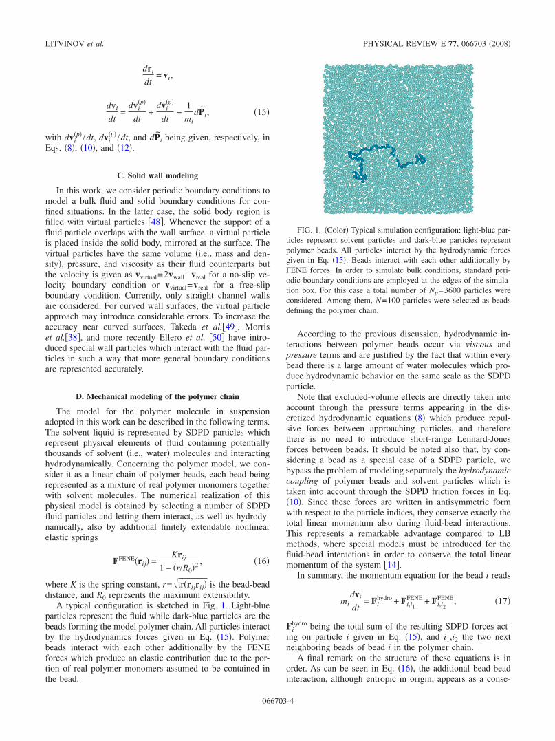
A typical configuration is sketched in Fig. 1. Light-blueparticles represent the fluid while dark-blue particles are thebeads forming the model polymer chain. All particles interactby the hydrodynamics forces given in Eq. �15�. Polymerbeads interact with each other additionally by the FENEforces which produce an elastic contribution due to the por-tion of real polymer monomers assumed to be contained inthe bead.

According to the previous discussion, hydrodynamic in-teractions between polymer beads occur via viscous andpressure terms and are justified by the fact that within everybead there is a large amount of water molecules which pro-duce hydrodynamic behavior on the same scale as the SDPDparticle.

Note that excluded-volume effects are directly taken intoaccount through the pressure terms appearing in the dis-cretized hydrodynamic equations �8� which produce repul-sive forces between approaching particles, and thereforethere is no need to introduce short-range Lennard-Jonesforces between beads. It should be noted also that, by con-sidering a bead as a special case of a SDPD particle, webypass the problem of modeling separately the hydrodynamiccoupling of polymer beads and solvent particles which istaken into account through the SDPD friction forces in Eq.�10�. Since these forces are written in antisymmetric formwith respect to the particle indices, they conserve exactly thetotal linear momentum also during fluid-bead interactions.This represents a remarkable advantage compared to LBmethods, where special models must be introduced for thefluid-bead interactions in order to conserve the total linearmomentum of the system �14�.

In summary, the momentum equation for the bead i reads

midvi

dt= Fi

hydro + Fi,i1FENE + Fi,i2

FENE, �17�

Fihydro being the total sum of the resulting SDPD forces act-

ing on particle i given in Eq. �15�, and i1,i2 the two nextneighboring beads of bead i in the polymer chain.

A final remark on the structure of these equations is inorder. As can be seen in Eq. �16�, the additional bead-beadinteraction, although entropic in origin, appears as a conse-

FIG. 1. �Color� Typical simulation configuration: light-blue par-ticles represent solvent particles and dark-blue particles representpolymer beads. All particles interact by the hydrodynamic forcesgiven in Eq. �15�. Beads interact with each other additionally byFENE forces. In order to simulate bulk conditions, standard peri-odic boundary conditions are employed at the edges of the simula-tion box. For this case a total number of Np=3600 particles wereconsidered. Among them, N=100 particles were selected as beadsdefining the polymer chain.

LITVINOV et al. PHYSICAL REVIEW E 77, 066703 �2008�

066703-4

quence of the GENERIC framework in the model Eq. �17� asan ordinary interparticle force �51�. Therefore, there is noparticular concern about the general structure of the modifiedSDPD model equations which is still consistent with the GE-NERIC model. In particular, the magnitudes of the stochasticterms are uniquely prescribed in terms of the dissipativeforces between the particles, which in this model remain un-altered.

III. NUMERICAL SETUP

In this work, the statistical properties of a single polymermolecule immersed in a Newtonian liquid under good sol-vent conditions are investigated in an infinite domain and ina confined geometry. In the first case, the simulation domainis represented by a 2D square box of physical length L=10−5 m. A total number Np=3600 of SDPD particles isused. Among them, N particles representing polymer beadsare selected and allowed to interact by the FENE forces. Nranges from 20 to 100. Concerning the input parameters en-tering the FENE model, we choose K=5.3 N m−1 and R0=4�r, where �r=1.66�10−7 m is the initial particle spac-ing �52�.

Fluid particles interact by the forces given in Eq. �15�with cutoff radius h=5.0�10−7 m, and the kernel functionused is a quintic spline kernel. This implies an average num-ber of 20 neighboring SDPD particles entering the interpola-tion process.

Depending on the particular case, periodic or solid bound-ary conditions are used. In the latter case, solid walls aremodeled by virtual particles as discussed in Sec. II. Themethod prevents particles penetrating the solid wall �imper-meability condition� and forces the tangential component ofthe fluid velocity to be exactly zero at the interface �no-slipcondition� �40�. The previous conditions are crucial in takinginto account hydrodynamic effects due to the confinement.

Concerning the solvent, we consider a Newtonian fluidcharacterized by a dynamic viscosity �=10−6 kg m−1 s−1

and �=103 kg m−3, and the fluid temperature is set to T=300 K. According to these parameters, the solvent is ide-ally good and collapse never occurs. Concerning the nu-merical integration of the equations of motion for the par-ticles, a second-order predictor-corrector scheme is used. Tomaintain numerical stability, a Courant-Friedrichs-Lewy timestep restriction based upon artificial sound speed �isothermalcompressibility�, body force, and viscous dissipation�38,53,54� is employed. When thermal fluctuations are intro-duced in the mesoscopic simulation, the time steps are fur-ther decreased to recover the correct kinetic temperature. Theartificial speed of sound of the solvent liquid keeps relativedensity fluctuations below 1% and models a quasi-incompressible fluid.

Statistical averages are computed by extracting indepen-dent polymer configurations. The production run is per-formed after an equilibration period �500–2000 time stepsdepending on the length of the polymer chain� in order toavoid spurious effects due to the initial nonrandom polymerconfiguration.

Finally, a remark on the numerical efficiency of themethod is in order. The operation count of SDPD, as for

DPD or any other particle method, scales as Np log Np whenproper linked-list cell algorithms are employed. However,the fact that the mass density �i must be evaluated for everyparticle before calculating the interaction forces makes it po-tentially slightly slower. Nevertheless, the conceptual andtechnical advantages gained from the thermodynamical con-sistency of SDPD and its direct connection to the Navier-Stokes equations overwhelm the performance penalty.

IV. SIMULATION RESULTS

In this section, the conformational properties of the poly-mer molecule are investigated in a two-dimensional space.The objective is twofold: First, we apply the SDPD methodto the study of a polymer molecule in an infinite solventmedium under zero-flow condition. In this case, the stochas-tic Wiener process entering Eq. �15� represents the only forc-ing term mimicking the presence of thermal fluctuations inthe system. Under these conditions, the flow is isotropic, andtheoretically predicted universal scaling laws for severalpolymer properties can be tested numerically. In particular,the static and dynamic behavior of the conformational poly-mer properties as well as the structure factor have been in-tensely studied using a variety of methods �9,10,14� and arecompared here with the present results.

Second, the effect of geometrical confinement, in particu-lar due to the presence of solid walls in microchannels, isinvestigated. This is an important validation test because itallows us to estimate the accuracy of SDPD in simulatingreal geometries encountered in microfluidic devices. It isgenerally known that confinement alters dramatically the be-havior of a polymer molecule which in a microchannel, forexample, will extend along the channel axis to a substantialfraction of its contour length. Scaling laws for the depen-dence of the polymer stretch upon the channel width havebeen proposed theoretically �37� and validated numericallyin a number of 3D situations. As a further test for the SDPDmethod, the two-dimensional static properties of a polymermolecule confined in a microchannel are investigated and theresults are compared with previous theoretical and numericalwork �12,20,36�.

A. Conformational properties of a polymer in a bulk medium

1. Chain statics

Conformational properties of a polymer chain, in particu-lar deformation and orientation, can be analyzed by monitor-ing the evolution of several tensorial quantities such as, forinstance the gyration tensor

G �1

2N2�i,j

�rijrij� , �18�

or the end-to-end tensor defined as

R � ��rN − r1��rN − r1�� . �19�

Here, rij =r j −ri with ri being the position of the ith bead inthe chain. The indices i,j run from 1 to N, the total number ofbeads. Related quantities are the radius of gyration RG

SMOOTEHED DISSIPATIVE PARTICLE DYNAMICS MODEL … PHYSICAL REVIEW E 77, 066703 �2008�

066703-5

= tr G and the end-to-end radius RE= tr R. The effect ofthe number of beads N on RG and RE is known to follow theanalytical expressions

RE = aE�N − 1��,

RG = aG��N2 − 1�/N��, �20�

where � is called the static factor exponent and, from renor-malization theory, it assumes the value ��0.588 in threedimensions, with aE and aG being suitable constants. In thelimiting case of N�1, both quantities scale as RE�RG�N�.Notice that this result is valid only in three dimensions. Be-cause the goal of this work is to test the numerical schemefirst in a 2D case, the static exponent � extracted by oursimulations should be compared with the analogous two-dimensional Flory formula, which gives a value 0.75 in goodsolvent conditions �37,55�. This value has been verified re-cently by several authors using molecular dynamics simula-tions �32–34�.

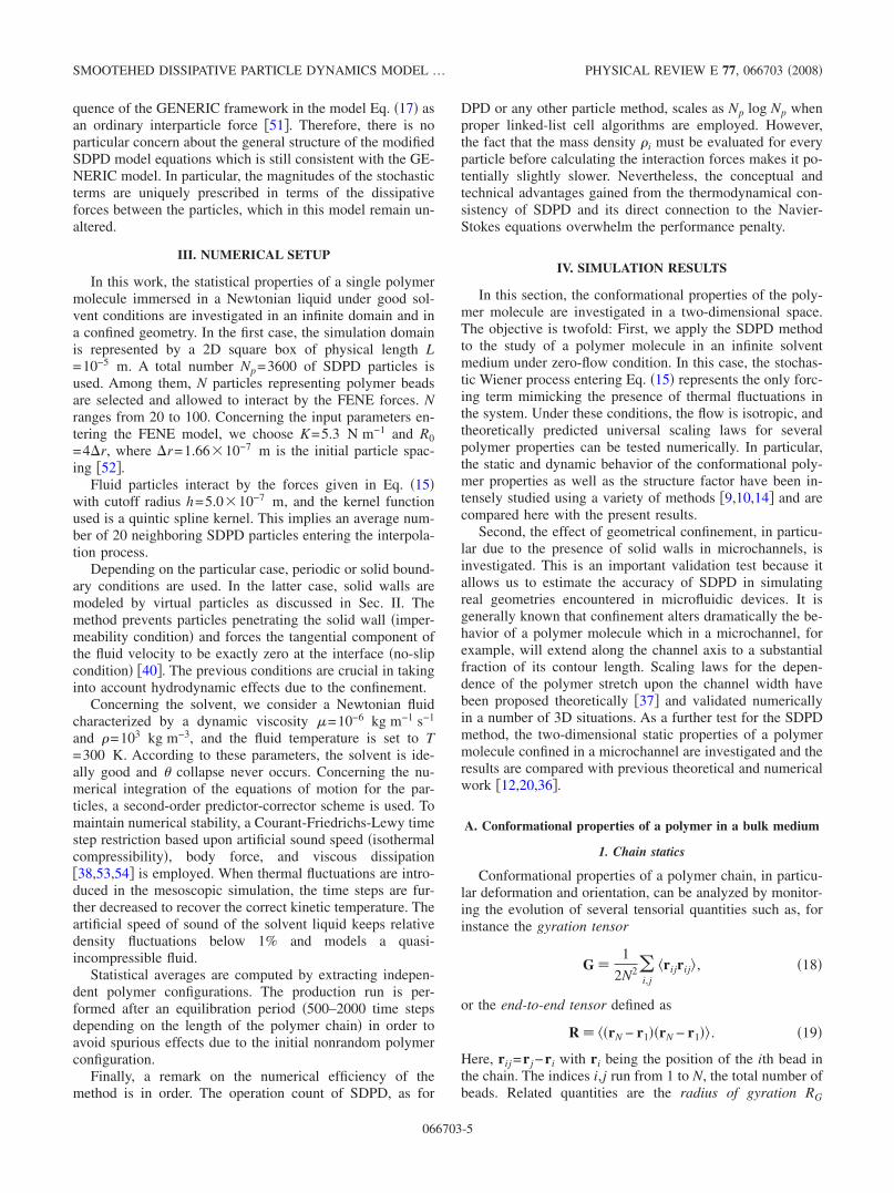
In order to extract the exponent �, SDPD simulationshave been carried out with five different chain lengths char-acterized by N=20,40,60,80,100 beads. In all cases thetime-averaged values of the gyration radius RG have beenevaluated from several independent steady-state polymerconfigurations. Figure 2 shows a log-log plot of the time-averaged RG versus N. Error bars are within the symbol di-mensions. The results can be fitted �dotted line in the figure�by a power law with exponent �=0.76�0.012, which is ingood agreement with theoretical results and previous numeri-cal investigations. It should be noticed that this way to evalu-ate � is quite time consuming since simulations at large N arenecessary in order to fit accurately the data in Fig. 2.

An alternative way to extract � is, instead of using thescaling law �20�, by employing the static structure factordefined as

S�k� �1

N�i,j

�exp�− ik · rij�� . �21�

In the limit of small wave vector kRG�1, the structurefactor can be approximated by S�k��N�1−k2RG /3�, while

for kRG�1 S�k��2N /k2RG holds. The intermediate re-gime kRG�1 contains information about the intramolecularspatial correlations. In the absence of external perturbationand close to equilibrium, S�k� is isotropic and therefore de-pends only on the magnitude of the wave vector k= k. S�k�probes therefore different length scales even for a singlepolymer, and in the intermediate regime is shown to behavelike

S�k� � k−1/�. �22�

Figure 3 shows a log-log plot of S�k� vs RGk. From thisfigure it is possible to see how curves evaluated from simu-lations with different chain lengths �N� collapse on a singlecurve for 2�RGk�8, the slope of the linear region being−1 /�. The dotted line in the figure represents the theory with�=0.75 and shows very good agreement with the SDPD re-sults.

This way provides a more efficient route to calculate thestatic exponent �, since one single simulation with N=20 issufficient for accurate estimates.

These two tests are commonly performed to validate theequilibrium conformational properties of a FENE polymermolecule. These scaling laws have been also verified byother techniques such as, for instance, DPD in three dimen-sions �17�.

2. Chain dynamics

The dynamic conformational behavior of the polymermolecule represents another important feature that must bechecked. The starting point is the dynamical structure factordefined as

S�k,t� �1

N�i,j

�exp�− ik · �ri�t� − r j�0���� . �23�

Dynamic scaling arguments applied to the Zimm model inisotropic conditions predict a functional form of S�k , t� of thetype

FIG. 2. Scaling of the radius of gyration RG for several chainlengths corresponding to N=20,30,40,50,60,80,100 beads. Thedotted line represents the best fit consistent with the theory �RG

�N�� and gives a static exponent �=0.76�0.012.

FIG. 3. Normalized equilibrium static structure factor S�k�=S�k� /S�0� versus RGk corresponding to several chain lengths. Allthe curves collapse on a master line for 2�RGk�8 �scaling re-

gime�. In this region S�k��k−1/� with �=0.75 �dotted line�.

LITVINOV et al. PHYSICAL REVIEW E 77, 066703 �2008�

066703-6

S�k,t� = N�kRG��−1/��F�tDGRG−2�kRG�x� �24�

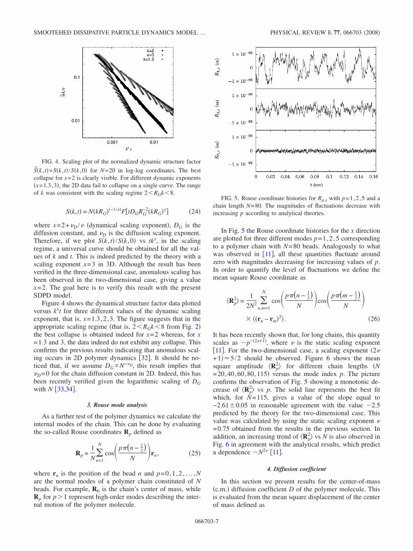
where x=2+�D /� �dynamical scaling exponent�, DG is thediffusion constant, and �D is the diffusion scaling exponent.Therefore, if we plot S�k , t� /S�k ,0� vs tkx, in the scalingregime, a universal curve should be obtained for all the val-ues of k and t. This is indeed predicted by the theory with ascaling exponent x=3 in 3D. Although the result has beenverified in the three-dimensional case, anomalous scaling hasbeen observed in the two-dimensional case, giving a valuex=2. The goal here is to verify this result with the presentSDPD model.

Figure 4 shows the dynamical structure factor data plottedversus kxt for three different values of the dynamic scalingexponent, that is, x=1.3,2 ,3. The figure suggests that in theappropriate scaling regime �that is, 2�RGk�8 from Fig. 2�the best collapse is obtained indeed for x=2 whereas, for x=1.3 and 3, the data indeed do not exhibit any collapse. Thisconfirms the previous results indicating that anomalous scal-ing occurs in 2D polymer dynamics �32�. It should be no-ticed that, if we assume DG�N−�D, this result implies that�D=0 for the chain diffusion constant in 2D. Indeed, this hasbeen recently verified given the logarithmic scaling of DGwith N �33,34�.

3. Rouse mode analysis

As a further test of the polymer dynamics we calculate theinternal modes of the chain. This can be done by evaluatingthe so-called Rouse coordinates Rp defined as

Rp =1

N�n=1

N

cos� p��n − 12�

N�rn, �25�

where rn is the position of the bead n and p=0,1 ,2 , . . . ,Nare the normal modes of a polymer chain constituted of Nbeads. For example, R0 is the chain’s center of mass, whileRp for p�1 represent high-order modes describing the inter-nal motion of the polymer molecule.

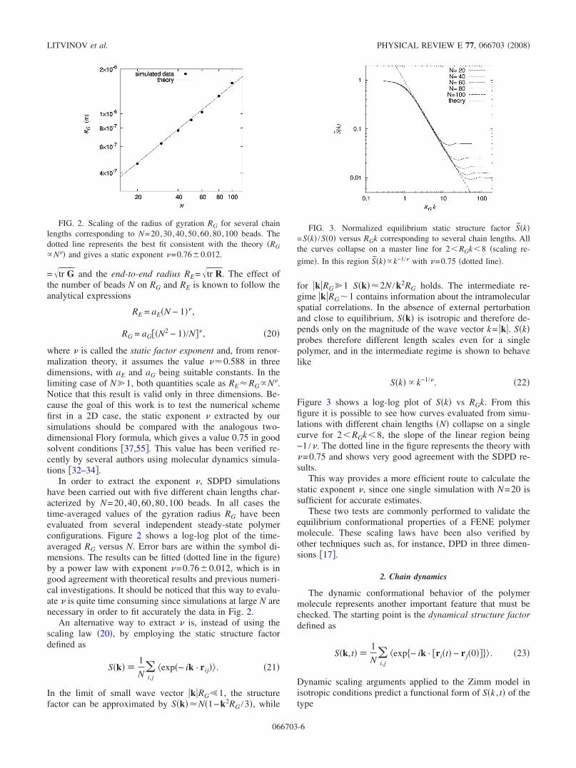
In Fig. 5 the Rouse coordinate histories for the x directionare plotted for three different modes p=1,2 ,5 correspondingto a polymer chain with N=80 beads. Analogously to whatwas observed in �11�, all these quantities fluctuate aroundzero with magnitudes decreasing for increasing values of p.In order to quantify the level of fluctuations we define themean square Rouse coordinate as

�Rp2� =

1

2N2 �n,m=1

N

cos� p��n − 12�

N�cos� p��m − 1

2�N

�� ��rn − rm�2� . �26�

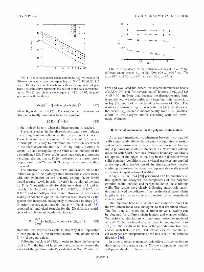
It has been recently shown that, for long chains, this quantityscales as �p−�2�+1�, where � is the static scaling exponent�11�. For the two-dimensional case, a scaling exponent �2�+1��5 /2 should be observed. Figure 6 shows the meansquare amplitude �Rp

2� for different chain lengths �N=20,40,60,80,115� versus the mode index p. The pictureconfirms the observation of Fig. 5 showing a monotonic de-crease of �Rp

2� vs p. The solid line represents the best fitwhich, for N=115, gives a value of the slope equal to−2.61�0.05 in reasonable agreement with the value �2.5predicted by the theory for the two-dimensional case. Thisvalue was calculated by using the static scaling exponent �=0.75 obtained from the results in the previous section. Inaddition, an increasing trend of �Rp

2� vs N is also observed inFig. 6 in agreement with the analytical results, which predicta dependence �N2� �11�.

4. Diffusion coefficient

In this section we present results for the center-of-mass�c.m.� diffusion coefficient D of the polymer molecule. Thisis evaluated from the mean square displacement of the centerof mass defined as

FIG. 4. Scaling plot of the normalized dynamic structure factor

S�k , t�=S�k , t� /S�k ,0� for N=20 in log-log coordinates. The bestcollapse for x=2 is clearly visible. For different dynamic exponents�x=1.3,3�, the 2D data fail to collapse on a single curve. The rangeof k was consistent with the scaling regime 2�RGk�8.

FIG. 5. Rouse coordinate histories for Rp,x with p=1,2 ,5 and achain length N=80. The magnitudes of fluctuations decrease withincreasing p according to analytical theories.

SMOOTEHED DISSIPATIVE PARTICLE DYNAMICS MODEL … PHYSICAL REVIEW E 77, 066703 �2008�

066703-7

��R0�t��2 = ��R0�t + t0� − R0�t0��2� �27�

where R0 is defined by �25�. The single-chain diffusion co-efficient is finally computed from the equation

��R0�t��2 = 4Dt �28�

in the limit of large t, when the linear regime is reached.Previous studies in the three-dimensional case indicate

that strong box-size effects in the evaluation of D occur.These finite-size corrections are of the order of 1 /L; hence,in principle, it is easy to determine the diffusion coefficientin the thermodynamic limit �L→�� by simply plotting Dversus 1 /L and extrapolating the value at the intercept of they coordinate �18�. These results have been shown to producea scaling relation, that is, D��N� collapses on a master curveproportional to N−�D, �D=0.59 being the dynamic scalingexponent.

The situation is more subtle in two dimensions due to theinfinite range of the hydrodynamic interactions. Consistencywith our evaluation of the dynamic scaling factor �x=0�would require �D=0. In order to verify it, we plotted the datafor D vs N logarithmically for different values of L and N,namely, N=10,20,40 and L=0.75�10−5 ,1.0�10−5 ,1.25�10−5, and no collapse was found. However, a decreasingscaling exponent �slope of the curves� was observed as thesystem size increased, analogously to previous findings �18�.In order to check quantitatively that �D=0, Falck et al. �33�.proposed an analytical formula for the 2D diffusion coeffi-cient of a polymer molecule which reads

D =kBT

2���− ln�Rg/L� + const + O„�Rg/L�2

…� . �29�

Note that this expression explains also why it is impossibleto extrapolate D in the thermodynamic limit, obtaining forL→� divergent values.

Following Falck et al. �33�, in order to check the behaviorof D vs N in the limit of large box sizes, we have inserted thevalues of the gyration radii Rg evaluated in Sec. IV into Eq.

�29� and evaluated the curves for several numbers of beadsN� �20:100� and for several cutoff lengths L=Lcut� �1.0�10−5 :10� m. Note that, because the thermodynamic limitis not defined, we select arbitrarily large but finite values Lcutin Eq. �29� and look at the trending behavior of D�N�. Theresults are shown in Fig. 7: as reported in �33�, the slopes ofthe curves ��D� decrease monotonically from 0.32 �smallestcutoff� to 0.04 �largest cutoff�, according with x=0 previ-ously evaluated.

B. Effect of confinement on the polymer conformation

As already mentioned, confinement between two parallelwalls significantly affects the polymer configuration statisticsand induces anisotropic effects. The situation is the follow-ing. A polymer molecule is immersed in a Newtonian solventmodeled with SDPD particles. Periodic boundary conditionsare applied at the edges of the box in the x direction whilesolid boundary conditions using virtual particles are appliedat the top and at the bottom of the simulation box therebyconfining the solvent between two impenetrable walls placeda distance H apart �channel width�.

Kong et al. in 1994 �20� performed DPD simulations ofthis system and analyzed the components of the polymergyration radius parallel and perpendicular to the confiningwalls. The results were clearly indicating anisotropic statis-tics and showed the collapse of the results for different chainlengths on a universal curve as a function of the normalizedchannel width.

The objective here is to validate our numerical model inthe two-dimensional case analogous to that described above.The first issue is to show that a similar universal scaling canbe obtained for different chain lengths and channel widths.We performed simulations with polymer molecules modeledwith N=20,60 beads and channel gaps H ranging from 1 to10 �m. The length of the box in the periodic direction waschosen such that Lx�4RG. This choice ensures that statisti-cal averages are independent of the box size in the periodicdirection �36�.

In order to observe an anisotropic effect it is convenient todecompose the gyration radius RG into components paralleland perpendicular to the walls as follows:

FIG. 6. Rouse mode mean square amplitudes �Rp2� vs mode p for

different polymer chains corresponding to N=20,40,60,80,115beads. The decrease of fluctuations with increasing value of p isclear. The solid curve represents the best fit of the data correspond-ing to N=115 and gives a slope equal to −2.61�0.05, in goodagreement with the theory.

FIG. 7. Dependence of the diffusion coefficient D on N fordifferent cutoff lengths Lcut in Eq. �29�: ��� Lcut=10−5 m, ���Lcut=10−3 m, ��� Lcut=10−1 m, and ��� Lcut=10 m.

LITVINOV et al. PHYSICAL REVIEW E 77, 066703 �2008�

066703-8

RG� =1

2N2�i,j

�xij2 �, RG� =

1

2N2�i,j

�yij2 � , �30�

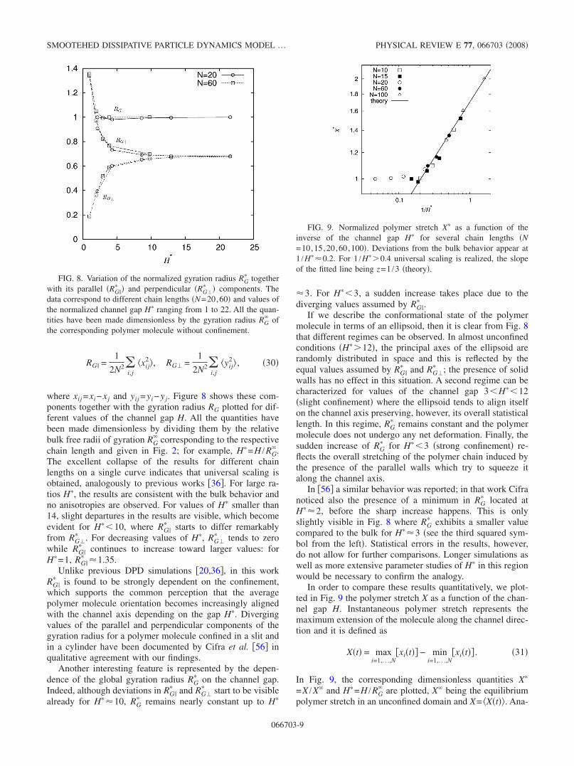
where xij =xi−xj and yij =yi−yj. Figure 8 shows these com-ponents together with the gyration radius RG plotted for dif-ferent values of the channel gap H. All the quantities havebeen made dimensionless by dividing them by the relativebulk free radii of gyration RG

� corresponding to the respectivechain length and given in Fig. 2; for example, H�=H /RG

�.The excellent collapse of the results for different chainlengths on a single curve indicates that universal scaling isobtained, analogously to previous works �36�. For large ra-tios H�, the results are consistent with the bulk behavior andno anisotropies are observed. For values of H� smaller than14, slight departures in the results are visible, which becomeevident for H��10, where RG�

� starts to differ remarkablyfrom RG�

� . For decreasing values of H�, RG�� tends to zero

while RG�� continues to increase toward larger values: for

H�=1, RG�� �1.35.

Unlike previous DPD simulations �20,36�, in this workRG�

� is found to be strongly dependent on the confinement,which supports the common perception that the averagepolymer molecule orientation becomes increasingly alignedwith the channel axis depending on the gap H�. Divergingvalues of the parallel and perpendicular components of thegyration radius for a polymer molecule confined in a slit andin a cylinder have been documented by Cifra et al. �56� inqualitative agreement with our findings.

Another interesting feature is represented by the depen-dence of the global gyration radius RG

� on the channel gap.Indeed, although deviations in RG�

� and RG�� start to be visible

already for H��10, RG� remains nearly constant up to H�

�3. For H��3, a sudden increase takes place due to thediverging values assumed by RG�

� .If we describe the conformational state of the polymer

molecule in terms of an ellipsoid, then it is clear from Fig. 8that different regimes can be observed. In almost unconfinedconditions �H��12�, the principal axes of the ellipsoid arerandomly distributed in space and this is reflected by theequal values assumed by RG�

� and RG�� ; the presence of solid

walls has no effect in this situation. A second regime can becharacterized for values of the channel gap 3�H��12�slight confinement� where the ellipsoid tends to align itselfon the channel axis preserving, however, its overall statisticallength. In this regime, RG

� remains constant and the polymermolecule does not undergo any net deformation. Finally, thesudden increase of RG

� for H��3 �strong confinement� re-flects the overall stretching of the polymer chain induced bythe presence of the parallel walls which try to squeeze italong the channel axis.

In �56� a similar behavior was reported; in that work Cifranoticed also the presence of a minimum in RG

� located atH��2, before the sharp increase happens. This is onlyslightly visible in Fig. 8 where RG

� exhibits a smaller valuecompared to the bulk for H��3 �see the third squared sym-bol from the left�. Statistical errors in the results, however,do not allow for further comparisons. Longer simulations aswell as more extensive parameter studies of H� in this regionwould be necessary to confirm the analogy.

In order to compare these results quantitatively, we plot-ted in Fig. 9 the polymer stretch X as a function of the chan-nel gap H. Instantaneous polymer stretch represents themaximum extension of the molecule along the channel direc-tion and it is defined as

X�t� = maxi=1,. . .,N

�xi�t�� − mini=1,. . .,N

�xi�t�� . �31�

In Fig. 9, the corresponding dimensionless quantities X�

=X /X� and H�=H /RG� are plotted, X� being the equilibrium

polymer stretch in an unconfined domain and X= �X�t��. Ana-

FIG. 8. Variation of the normalized gyration radius RG� together

with its parallel �RG�� � and perpendicular �RG�

� � components. Thedata correspond to different chain lengths �N=20,60� and values ofthe normalized channel gap H� ranging from 1 to 22. All the quan-tities have been made dimensionless by the gyration radius RG

� ofthe corresponding polymer molecule without confinement.

FIG. 9. Normalized polymer stretch X� as a function of theinverse of the channel gap H� for several chain lengths �N=10,15,20,60,100�. Deviations from the bulk behavior appear at1 /H��0.2. For 1 /H��0.4 universal scaling is realized, the slopeof the fitted line being z=1 /3 �theory�.

SMOOTEHED DISSIPATIVE PARTICLE DYNAMICS MODEL … PHYSICAL REVIEW E 77, 066703 �2008�

066703-9

lytical theories predict scaling behavior and give X�

� �H���−2/3� in a 3D square channel of width H�. Recently,these results have been validated numerically by Jendrejacket al. using Brownian dynamics techniques �12�, showing agood agreement with the de Gennes theory in 3D. Figure 9shows the analogous scenario in a two-dimensional case fordifferent chain lengths N=10,15,20,60,100. Excellent scal-ing behavior is obtained. Similarly to what is observed in�12�, X� remains constant up to values of 1 /H� approxi-mately equal to 0.2 where confinement effects start to bevisible, while for 1 /H��0.4 the scaling regime is fully real-ized. The slope of the approximate fitted curve prescribes ascaling law H��−z� where z=1 /3 in good agreement with thethe Gennes theory in two dimensions. Notice that the previ-ous result differs from the 3D case studied by Jendrejack etal. �57� where the scaling exponent takes a value equal to2/3.

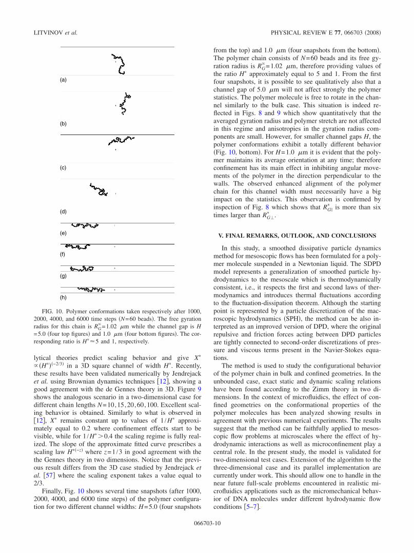
Finally, Fig. 10 shows several time snapshots �after 1000,2000, 4000, and 6000 time steps� of the polymer configura-tion for two different channel widths: H=5.0 �four snapshots

from the top� and 1.0 �m �four snapshots from the bottom�.The polymer chain consists of N=60 beads and its free gy-ration radius is RG

� =1.02 �m, therefore providing values ofthe ratio H� approximately equal to 5 and 1. From the firstfour snapshots, it is possible to see qualitatively also that achannel gap of 5.0 �m will not affect strongly the polymerstatistics. The polymer molecule is free to rotate in the chan-nel similarly to the bulk case. This situation is indeed re-flected in Figs. 8 and 9 which show quantitatively that theaveraged gyration radius and polymer stretch are not affectedin this regime and anisotropies in the gyration radius com-ponents are small. However, for smaller channel gaps H, thepolymer conformations exhibit a totally different behavior�Fig. 10, bottom�. For H=1.0 �m it is evident that the poly-mer maintains its average orientation at any time; thereforeconfinement has its main effect in inhibiting angular move-ments of the polymer in the direction perpendicular to thewalls. The observed enhanced alignment of the polymerchain for this channel width must necessarily have a bigimpact on the statistics. This observation is confirmed byinspection of Fig. 8 which shows that RG�

� is more than sixtimes larger than RG�

� .

V. FINAL REMARKS, OUTLOOK, AND CONCLUSIONS

In this study, a smoothed dissipative particle dynamicsmethod for mesoscopic flows has been formulated for a poly-mer molecule suspended in a Newtonian liquid. The SDPDmodel represents a generalization of smoothed particle hy-drodynamics to the mesoscale which is thermodynamicallyconsistent, i.e., it respects the first and second laws of ther-modynamics and introduces thermal fluctuations accordingto the fluctuation-dissipation theorem. Although the startingpoint is represented by a particle discretization of the mac-roscopic hydrodynamics �SPH�, the method can be also in-terpreted as an improved version of DPD, where the originalrepulsive and friction forces acting between DPD particlesare tightly connected to second-order discretizations of pres-sure and viscous terms present in the Navier-Stokes equa-tions.

The method is used to study the configurational behaviorof the polymer chain in bulk and confined geometries. In theunbounded case, exact static and dynamic scaling relationshave been found according to the Zimm theory in two di-mensions. In the context of microfluidics, the effect of con-fined geometries on the conformational properties of thepolymer molecules has been analyzed showing results inagreement with previous numerical experiments. The resultssuggest that the method can be faithfully applied to mesos-copic flow problems at microscales where the effect of hy-drodynamic interactions as well as microconfinement play acentral role. In the present study, the model is validated fortwo-dimensional test cases. Extension of the algorithm to thethree-dimensional case and its parallel implementation arecurrently under work. This should allow one to handle in thenear future full-scale problems encountered in realistic mi-crofluidics applications such as the micromechanical behav-ior of DNA molecules under different hydrodynamic flowconditions �5–7�.

(b)

(a)

(c)

(d)

(f)

(e)

(g)

(h)

FIG. 10. Polymer conformations taken respectively after 1000,2000, 4000, and 6000 time steps �N=60 beads�. The free gyrationradius for this chain is RG

� =1.02 �m while the channel gap is H=5.0 �four top figures� and 1.0 �m �four bottom figures�. The cor-responding ratio is H��5 and 1, respectively.

LITVINOV et al. PHYSICAL REVIEW E 77, 066703 �2008�

066703-10

A final discussion on the Schmidt number is in order. TheSchmidt number is defined as Sc=� /D, where � is the kine-matic viscosity of the solvent and D the molecular diffusiv-ity. Strictly speaking, the applicability of the Zimm theoryfor the polymer dynamics requires Sc to be much larger thanone. For instance, in a real liquid like water Sc�1000. Thiscondition implies that mass diffusion is much slower thanmomentum diffusion, and this is crucial for the validity ofthe Oseen tensor approximation. In the present work, theSchmidt number evaluated by the input kinematic viscosityand the numerically estimated fluid particle diffusivity is, asin DPD, of order 1. Nevertheless, scaling relations for thepolymer dynamics have been recovered in good agreement

with the Zimm theory with full hydrodynamic interactions.These results confirm the fact, already suggested by someauthors �18,58�, that the Schmidt number is an ill-definedquantity for coarse-graining models. There is therefore noneed in principle to increase Sc but numbers of O�1� can stillproduce the correct hydrodynamic behavior and, at the sametime, provide a reasonable choice in terms of CPU time. Inorder to increase the artificial Schmidt number, a way wouldbe to increase the kinematic viscosity with a numericalbottleneck due to the viscous time step limitation as a con-sequence. Realistic conditions could, however, be reached byusing implicit schemes like those presented in �59,60�, whichare currently under investigation.

�1� G. E. Karniadakis and A. Beskok, Micro Flows, Fundamentalsand Simulations �Springer, New York, 2002�.

�2� S. C. Glotzer and W. Paul, Annu. Rev. Mater. Res. 32, 401�2002�.

�3� A. Uhlherr and D. N. Theodorou, Curr. Opin. Solid StateMater. Sci. 3, 544 �1998�.

�4� H. A. Stone and S. Kim, AIChE J. 47, 1250 �2001�.�5� M. Mertig, L. Colombi, R. Seidel, W. Pompe, and A. De Vita,

Nano Lett. 2, 841 �2002�.�6� S. Diez, C. Reuther, C. Dinu, R. Seidel, M. Mertig, W. Pompe,

and J. Howard, Nano Lett. 3, 1251 �2003�.�7� M. Mertig, L. Colombi, A. Benke, A. Huhle, J. Opitz, R.

Seidel, H. K. Schackert, and W. Pompe, in Foundations ofNanoscience: Self-Assembled Architectures and Devices, ed-ited by J. Reif �Science Technica, Snowbird, Utah, 2004�, p.132.

�8� L. D. Landau and E. M. Lifschitz, Fluid Mechanics �PergamonPress, New York, 1959�.

�9� B. Dünweg and K. Kremer, J. Chem. Phys. 99, 6983 �1993�.�10� C. Aust, M. Kröger, and S. Hess, Macromolecules 32, 5660

�1999�.�11� J. M. Polson and J. P. Gallant, J. Chem. Phys. 124, 184905

�2006�.�12� R. Jendrejack, D. C. Schwartz, M. D. Graham, and J. J. de

Pablo, J. Chem. Phys. 119, 1165 �2003�.�13� K. Mussawisade, M. Ripoll, R. G. Winkler, and G. Gomper, J.

Chem. Phys. 123, 144905 �2005�.�14� P. Ahlrichs and B. Dünweg, J. Chem. Phys. 111, 8225 �1999�.�15� P. J. Hoogerbrugge and J. Koelman, Europhys. Lett. 19, 155

�1992�.�16� P. Español and P. Warren, Europhys. Lett. 30, 191 �1995�.�17� N. A. Spenley, Europhys. Lett. 49, 534 �2000�.�18� W. Jiang, J. Huang, Y. Wang, and M. Laradji, J. Chem. Phys.

126, 044901 �2007�.�19� V. Symeonidis, G. E. Karniadakis, and B. Caswell, Phys. Rev.

Lett. 95, 076001 �2005�.�20� Y. Kong, C. W. Manke, W. G. Madden, and A. G. Schlijper,

Tribol. Lett. 3, 133 �1997�.�21� S. Chen, N. Phan-Thien, X.-J. Fan, and B. C. Khoo, J. Non-

Newtonian Fluid Mech. 118, 65 �2004�.�22� X. Fan, N. Phan-Thien, and S. Chen, Phys. Fluids 18, 063102

�2006�.

�23� X. Fan, N. Phan-Thien, and T. Ng, Phys. Fluids 15, 11 �2003�.�24� The use of soft two-body potentials in DPD may allow for

chain crossing �violating topological constraints �18�� as wellas particle penetration to the walls in problems involving con-fined situations.

�25� P. Español and M. Revenga, Phys. Rev. E 67, 026705 �2003�.�26� J. J. Monaghan, Annu. Rev. Astron. Astrophys. 30, 543

�1992�.�27� R. A. Gingold and J. J. Monaghan, Mon. Not. R. Astron. Soc.

181, 375 �1977�.�28� L. B. Lucy, Astron. J. 82, 1013 �1977�.�29� J. M. Vianney and A. Koelman, Phys. Rev. Lett. 64, 1915

�1990�.�30� B. Maier and J. O. Rädler, Phys. Rev. Lett. 82, 1911 �1999�.�31� R. Azuma and H. Takayama, J. Chem. Phys. 111, 8666 �1999�.�32� S. R. Shannon and T. C. Choy, Phys. Rev. Lett. 79, 1455

�1997�.�33� E. Falck, O. Punkkinen, I. Vattulainen, and T. Ala-Nissila,

Phys. Rev. E 68, 050102�R� �2003�.�34� O. Punkkinen, E. Falck, I. Vattulainen, and T. Ala-Nissila, J.

Chem. Phys. 122, 094904 �2005�.�35� A. Milchev and K. Binder, J. Phys. II 6, 21 �1996�.�36� Y. Kong, C. W. Manke, W. G. Madden, and A. G. Schlijper,

Int. J. Thermophys. 15�6�, 1093 �1994�.�37� P. G. de Gennes, Scaling Concepts in Polymer Physics �Cor-

nell University Press, Ithaca, NY, 1979�.�38� J. P. Morris, P. J. Fox, and Y. Zhu, J. Comput. Phys. 136, 214

�1997�.�39� J. P. Morris, Int. J. Numer. Methods Fluids 33, 333 �2000�.�40� X. Y. Hu and N. A. Adams, J. Comput. Phys. 213, 844 �2006�.�41� Note that, unlike DPD, SDPD repulsive interparticle forces

have a multibody character due to the dependency of the pres-sure term Pi on the local value of the particle density �i

=� jmjWij. This is a remarkable property of the method whichprevents particle crossing for monomers and confining walls.

�42� E. G. Flekkøy, P. V. Coveney, and G. de Fabritiis, Phys. Rev. E62, 2140 �2000�.

�43� J. Bonet and T.-S. L. Lok, Comput. Methods Appl. Mech. Eng.180, 97 �1999�.

�44� M. Ellero, P. Español, and E. G. Flekkøy, Phys. Rev. E 68,041504 �2003�.

�45� M. Grmela and H. C. Öttinger, Phys. Rev. E 56, 6620 �1997�.

SMOOTEHED DISSIPATIVE PARTICLE DYNAMICS MODEL … PHYSICAL REVIEW E 77, 066703 �2008�

066703-11

�46� H. C. Öttinger and M. Grmela, Phys. Rev. E 56, 6633 �1997�.�47� P. Español, M. Serrano, and H. C. Öttinger, Phys. Rev. Lett.

83, 4542 �1999�.�48� P. W. Randles and L. D. Libersky, Mech. Eng. 139, 375

�1996�.�49� H. Takeda, S. M. Miyama, and M. Sekiya, Prog. Theor. Phys.

92, 939 �1994�.�50� M. Ellero, M. Kröger, and S. Hess, Multiscale Model. Simul.

5, 759 �2006�.�51� P. Español �private communication�.�52� Notice that the FENE polymer molecule introduces an addi-

tional length in the model. The contour length is an appropriateparameter to estimate this molecular size. According to �23�, ifLc denotes one segment of the molecular chain, its averagevalue is of the order of R0

2 / �b+5�, where b=KR02 / �kBT� is a

dimensionless parameter approximately equal to 95 in oursimulations. This gives Lc�6.6�10−2 �m. The polymer con-

tour length will be therefore L=NLc and assumes values rang-ing from �1.3 �m �N=20� to �7 �m �N=100� consistentwith the contour lengths of �-DNA molecules.

�53� M. Ellero, M. Kröger, and S. Hess, J. Non-Newtonian FluidMech. 105, 35 �2002�.

�54� M. Ellero and R. I. Tanner, J. Non-Newtonian Fluid Mech.132, 61 �2005�.

�55� M. Doi and S. F. Edwards, The Theory of Polymer Dynamics�Clarendon, Oxford, 1986�.

�56� P. Cifra and T. Bleha, Macromol. Theory Simul. 8, 603 �1999�.�57� R. Jendrejack, D. C. Schwartz, M. D. Graham, and J. J. de

Pablo, J. Chem. Phys. 120, 2513 �2004�.�58� E. A. J. F. Peters, Europhys. Lett. 66, 311 �2004�.�59� S. C. Whitehouse, M. R. Bate, and J. J. Monaghan, Mon. Not.

R. Astron. Soc. 364, 1367 �2005�.�60� T. Shardlow, SIAM J. Sci. Comput. 24, 1267 �2003�.

LITVINOV et al. PHYSICAL REVIEW E 77, 066703 �2008�

066703-12