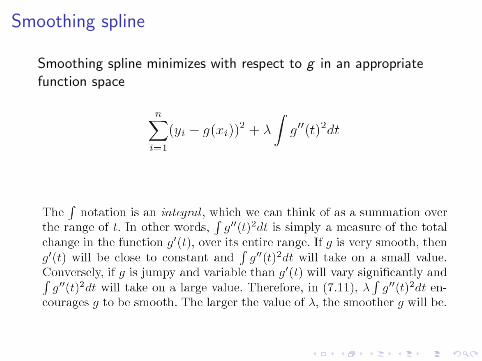
Smoothing spline

Smoothing spline minimizes with respect to g in an appropriatefunction space

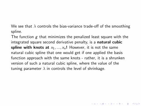
We see that λ controls the bias-variance trade-off of the smoothingspline.The function g that minimizes the penalized least square with theintegrated square second derivative penalty, is a natural cubicspline with knots at x1, ..., xn! However, it is not the samenatural cubic spline that one would get if one applied the basisfunction approach with the same knots - rather, it is a shrunkenversion of such a natural cubic spline, where the value of thetuning parameter λ in controls the level of shrinkage.

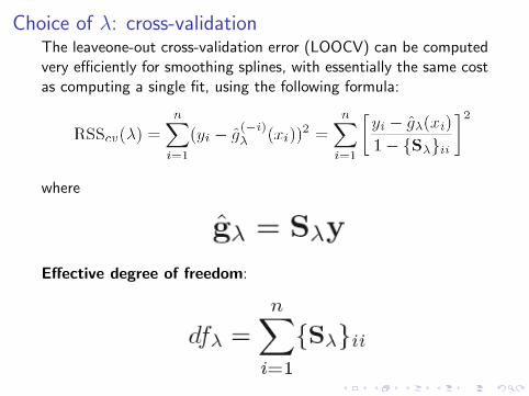
Choice of λ: cross-validationThe leaveone-out cross-validation error (LOOCV) can be computedvery efficiently for smoothing splines, with essentially the same costas computing a single fit, using the following formula:

where

Effective degree of freedom:

20 30 40 50 60 70 80

050

100

200

300

Age

Wage

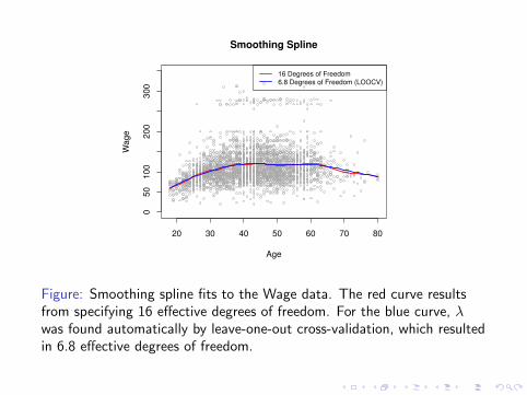
Smoothing Spline

16 Degrees of Freedom

6.8 Degrees of Freedom (LOOCV)

Figure: Smoothing spline fits to the Wage data. The red curve resultsfrom specifying 16 effective degrees of freedom. For the blue curve, λwas found automatically by leave-one-out cross-validation, which resultedin 6.8 effective degrees of freedom.

Local regression

0.0 0.2 0.4 0.6 0.8 1.0

−1

.0−

0.5

0.0

0.5

1.0

1.5

O

O

O

O

O

OO

O

O

O

O

O

O

O

O

OOO

O

O

O

O

O

O

O

O

OO

O

O

OO

O

O

O

O

O

O

OO

O

O

O

O

O

O

O

O

O

O

OO

O

O

O

O

O

OO

O

O

O

O

OO

O

O

OO

O

O

O

OO

O

O

O

O

O

O

O

OO

O

O

O

OO

O

O

O

O

OO

O

O

O

O

O

O

O

O

O

O

O

OO

O

O

O

O

O

O

O

O

OOO

O

O

O

O

0.0 0.2 0.4 0.6 0.8 1.0

−1

.0−

0.5

0.0

0.5

1.0

1.5

O

O

O

O

O

OO

O

O

O

O

O

O

O

O

OOO

O

O

O

O

O

O

O

O

OO

O

O

OO

O

O

O

O

O

O

OO

O

O

O

O

O

O

O

O

O

O

OO

O

O

O

O

O

OO

O

O

O

O

OO

O

O

OO

O

O

O

OO

O

O

O

O

O

O

O

OO

O

O

O

OO

O

O

O

O

OO

O

O

O

O

O

O

O

O

O

O

O

OO

O

O

OO

O

O

O

O

O

O

OO

O

O

O

O

O

O

O

O

O

O

OO

O

O

O

O

O

OO

O

O

O

O

OO

O

O

OO

O

O

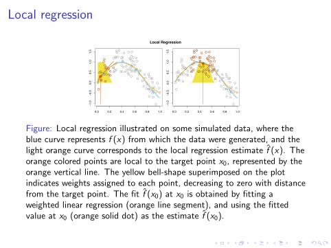
Local Regression

Figure: Local regression illustrated on some simulated data, where theblue curve represents f (x) from which the data were generated, and thelight orange curve corresponds to the local regression estimate f̂ (x). Theorange colored points are local to the target point x0, represented by theorange vertical line. The yellow bell-shape superimposed on the plotindicates weights assigned to each point, decreasing to zero with distancefrom the target point. The fit f̂ (x0) at x0 is obtained by fitting aweighted linear regression (orange line segment), and using the fittedvalue at x0 (orange solid dot) as the estimate f̂ (x0).

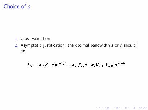
Choice of s

1. Cross validation

2. Asymptotic justification: the optimal bandwidth s or h shouldbe

20 30 40 50 60 70 80

050

100

200

300

Age

Wage

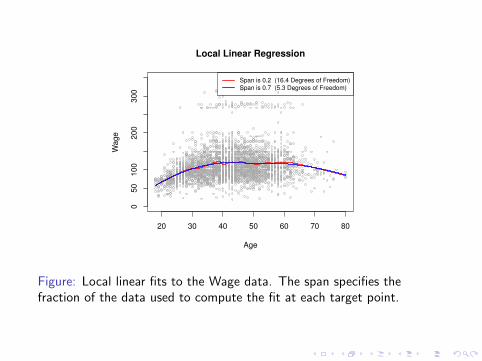
Local Linear Regression

Span is 0.2 (16.4 Degrees of Freedom)

Span is 0.7 (5.3 Degrees of Freedom)

Figure: Local linear fits to the Wage data. The span specifies thefraction of the data used to compute the fit at each target point.

Issues with local regression

I Computationally intensive. The weighted least square has beto fit for every x0.

I As the nearest neighbor method, it suffers ”the curse ofdimensionality”.

Generalized additive models (GAM): regression

2003 2005 2007 2009

−30

−20

−10

010

20

30

20 30 40 50 60 70 80

−50

−40

−30

−20

−10

010

20

−30

−20

−10

010

20

30

40

<HS HS <Coll Coll >Coll

f 1(year)

f 2(age)

f 3(edu

cation)

year ageeducation

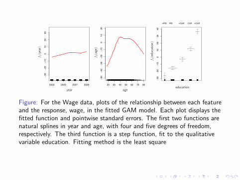
Figure: For the Wage data, plots of the relationship between each featureand the response, wage, in the fitted GAM model. Each plot displays thefitted function and pointwise standard errors. The first two functions arenatural splines in year and age, with four and five degrees of freedom,respectively. The third function is a step function, fit to the qualitativevariable education. Fitting method is the least square

2003 2005 2007 2009

−30

−20

−10

010

20

30

20 30 40 50 60 70 80

−50

−40

−30

−20

−10

010

20

−30

−20

−10

010

20

30

40

<HS HS <Coll Coll >Coll

f 1(year)

f 2(age)

f 3(edu

cation)

year ageeducation

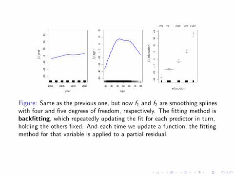
Figure: Same as the previous one, but now f1 and f2 are smoothing splineswith four and five degrees of freedom, respectively. The fitting method isbackfitting, which repeatedly updating the fit for each predictor in turn,holding the others fixed. And each time we update a function, the fittingmethod for that variable is applied to a partial residual.

Advantanges of GAM

I We do not have to use splines as the building blocks forGAMs: we can just as well use local regression, polynomialregression, or any combination of the approaches seen earlierin this chapter.

I GAMs allow us to fit a non-linear fj each Xj , so that we canautomatically model non-linear relationships that standardlinear regression will miss.

I The non-linear fits can potentially make more accuratepredictions for the response Y .

I Because the model is additive, we can still examine the effectof each Xj on Y individually while holding all of the othervariables fixed. Hence if we are interested in inference, GAMsprovide a useful representation.

I The smoothness of the function fj for the variable Xj can besummarized via degrees of freedom, which allows for inference.

I For fully general models, we have to look for even moreflexible approaches such as random forests and boosting,described in Chapter 8. GAMs provide a useful compromisebetween linear and fully nonparametric models.

Disadvantages of GAM

I The main limitation of GAMs is that the model is restricted tobe additive. With many variables, important interactions canbe missed. However, as with linear regression, we canmanually add interaction terms to the GAM model byincluding additional predictors of the form XjXk . In additionwe can add low-dimensional interaction functions of the formfjk(Xj ,Xk) into the model; such terms can be fit usingtwo-dimensional smoothers such as local regression, ortwo-dimensional splines

Generalized additive models (GAM): classification

2003 2005 2007 2009

−4

−2

02

4

20 30 40 50 60 70 80

−8

−6

−4

−2

02

−4

00

−2

00

02

00

40

0

<HS HS <Coll Coll >Coll

f 1(year)

f 2(age)

f 3(edu

cation)

year ageeducation

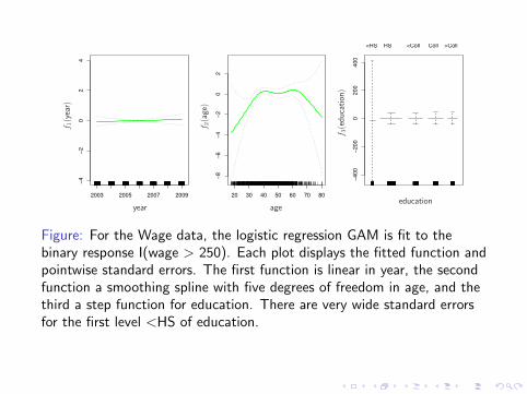
Figure: For the Wage data, the logistic regression GAM is fit to thebinary response I(wage > 250). Each plot displays the fitted function andpointwise standard errors. The first function is linear in year, the secondfunction a smoothing spline with five degrees of freedom in age, and thethird a step function for education. There are very wide standard errorsfor the first level <HS of education.

2003 2005 2007 2009

−4

−2

02

4

20 30 40 50 60 70 80

−8

−6

−4

−2

02

−4

−2

02

4

HS <Coll Coll >Coll

f 1(year)

f 2(age)

f 3(edu

cation)

year ageeducation

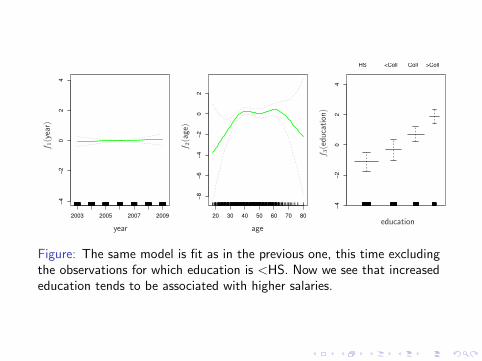
Figure: The same model is fit as in the previous one, this time excludingthe observations for which education is <HS. Now we see that increasededucation tends to be associated with higher salaries.