Smoothness Testing of Polynomials over Finite Fields

Jean-Francois Biasse and Michael J. Jacobson Jr.

Department of Computer Science, University of Calgary2500 University Drive NW

Calgary, Alberta, Canada T2N 1N4

Abstract

We present an analysis of Bernstein’s batch integer smoothness test when applied to thecase of polynomials over a finite field Fq. We compare the performance of our algorithmwith the standard method based on distinct degree factorization from both an analyticaland a practical point of view. Our results show that the batch test offers no advantageasymptotically, and that it offers practical improvements only in a few rare cases.

1 Introduction

Smoothness testing is an essential part of many modern algorithms, including index-calculus al-gorithms for a variety of applications. Algorithms for integer factorization, discrete logarithmsin finite fields of large characteristic, and computing class groups and fundamental units of num-ber fields require smoothness testing of integers. Testing polynomials over finite fields for t-smoothness, i.e., determining whether all irreducible factors have degree less than or equal to t, isalso important in other settings. For example, the relation search performed to solve the discretelogarithm problem in the Jacobian of a genus g hyperelliptic curve over a finite field Fq by theEnge-Gaudry method [7] requires testing of a large amount of degree-g polynomials over Fq fort-smoothness. Smoothness testing of polynomials is also used in the cofactorization stage of siev-ing algorithms in function fields (see [11] for a survey mentioning their relevance to the discretelogarithm in finite fields). The sieve selects candidate polynomials over F2 that are likely to besmooth, and then these are rigorously tested for smoothness. The discrete logarithm problem inthe Jacobian of a hyperelliptic curve over Fq can also be solved by using sieving methods [14] inan analogous manner.

In [2], Bernstein presented an algorithm to test the smoothness of a batch of integers thatruns in time O

(b(log b)2 log log b

), where b is the total number of input bits. This represents a

significant improvements over the elliptic curve method described by Lenstra [9] which is conjec-

tured to work in time O(be√

(2+o(1)) log(b) log log(b)). This method has been used successfully in anumber of contexts, for example by Bisson and Sutherland as part of an algorithm for computingthe endomorphism ring of an elliptic curve over a finite field [4] and by the authors for computingclass groups in quadratic fields [3].

Bernstein’s algorithm can be adapted easily for smoothness testing of polynomials over finitefields. However, it is not clear how much of a practical impact the resulting algorithm would havebecause, unlike the integer case, testing a polynomial over Fq for t-smoothness can be done inpolynomial time with respect to the input, as described by Coppersmith [5]. Several variants ofCoppersmith’s method exist and are used in practice; we refer to the one described by Jacobson,Menezes and Stein [8]. When using “schoolbook” polynomial arithmetic, the number of fieldmultiplications required for this method is in O(d2t log q + d2+ε) where d is the degree of thepolynomial to be tested. With asymptotically faster algorithms, this improves to O(d1+εt log q).

1

The main idea of Bernstein’s algorithm is to test a batch of polynomials for smoothness simul-taneously. The product of these polynomials is first computed, followed by a “remainder tree”,resulting in the product of all irreducible of degree t or less modulo each individual polynomial.Those that result in zero are t-smooth. The point is that much of the arithmetic is done with verylarge degree polynomials where the asymptotically fastest algorithms for polynomial arithmeticwork best. When compared with Coppersmith’s method, where the single polynomial operandshave relatively small degree, the hope is that the use of these asymptotically faster algorithmsresults in an improved amortized cost.

In this paper, we describe our adaptation of Bernstein’s algorithm for smoothness testing ofpolynomials over Fq and compare its performance with that of Jacobson, Menezes and Stein [8].We show that the amortized number of field operations is in O

(dt log(q) + d1+ε

), almost the

same as that of the standard method. We present numerical results obtained with a C++ imple-mentation based on the libraries GMP, GF2X, and NTL confirming our analysis (implementationis available upon request). We test our algorithm on a number of examples of practical relevanceand show that the batch algorithm does not offer an improvement.

In Section 2, we briefly review the main polynomial multiplication and remainder algorithmsand their complexities in terms of field operations. We recall Coppersmith’s smoothness test, asdescribed in [8] in Section 3, and give a complexity analysis. In the next section we describe ouradaptation of Bernstein’s algorithm to polynomials over finite fields, followed by its complexityanalysis. We conclude with numerical results demonstrating the algorithm’s performance inpractice.

2 Arithmetic of polynomials

Let A,B ∈ Fq[x] where deg(A) = a, deg(B) = b with a ≥ b, and q = pm where p is a prime. Weexpress operation costs in terms of the number of multiplications in Fq, as a function of a and b,required to perform the operation.

Most implementations of polynomial arithmetic use multiple algorithms, selecting the mostefficient one based on the degrees of the operands. Our subsequent analysis considers three algo-rithms, the basic “schoolbook” method, the Karatsuba method, and a sub-quadratic complexityalgorithm using fast Fourier transform (FFT).

The “schoolbook” method has the following costs:

• computing AB requires (a+ 1)(b+ 1) multiplications in Fq;

• computing A mod B requires (b+ 1)(a− b+ 1) multiplications in Fq.

Asymptotically, both algorithms have complexityO(d2). The Karatsuba method requiresO(dlog2 3)field multiplications. The Schonhage-Strassen method [12] based on the Fast Fourier Transform(FFT) requires O(d log(d) log log(d)) field multiplications where d = max(a, b).

Fast multiplication allows a fast remainder operation via Newton division running in time2.5M(2(a − b + 1)) +M(2b) where M(d) is the cost of the multiplication between two degree-d polynomials. In particular, the cost of reducing a degree-2d polynomial modulo a degree-d polynomial is approximately 3.5M(d). Combined with the FFT, this gives us a remainderalgorithm running in time O(d log(d) log log(d)) where d = max(b, a− b).

Asymptotically, we will write the cost of multiplication and remainder computation as O(dθ)for some real constant theta 1 < θ ≤ 2 depending on the particular algorithm used. For theschoolbook algorithms we have θ = 2, for Karatsuba θ = log2 3, and for FFT we can take θ > 1arbitrarily small. Similarly, we will use O(dε) to denote logarithmic functions of d.

2

3 Smoothness Testing of Single Divisors

To assess the impact of our batch smoothness test for polynomials, we need a rigorous analysisof Coppersmith’s method that incorporates practical improvements such as those described byJacobson, Menezes and Stein [8]. In this section, we remind the reader of this method and providean analysis of the cost according to the framework defined in Section 2.

Suppose we have a polynomial N of degree d and that we want to determine whether N ist-smooth. A well-known fact about polynomials over Fq is that xq

i − x is equal to the productof all irreducible polynomials of degree dividing i (see for example [10]). This observation can beused in an analogue manner to efficient distinct-degree factorization algorithms for an efficientsmoothness-testing algorithm as follows:

1. Let l = bt/2c. Compute H = (xql+1 − x)(xq

l+1 − x) . . . (xqt − x) (mod N).

2. Compute H = Hd (mod N).

3. If H = 0, then N is t-smooth.

If N is t-smooth and square-free, then H = 0 after Step 1, since H is divisible by all polynomialsof degree ≤ t. The second step checks whether H is divisible by all polynomials of degree ≤ twith multiplicity deg(N), so any factors of N occurring to high powers will be detected.

The smoothness-testing algorithm is presented in Algorithm 1. In order to facilitate thesubsequent analysis, this algorithm is presented in detail.

Algorithm 1 Coppersmith Smoothness Test

Input: N ∈ Fq[x] with deg(N) = d, t ∈ ZOutput: “yes” if N is t-smooth, “no” otherwise1: {Compute P = xq

bt/2c(mod N)}

2: Set l = bt/2c.3: P = xq (mod N))4: for i = 1 to l do5: Compute P = P q (mod N)6: end for7: {Compute H = (xq

l+1 − x)(xql+1 − x) . . . (xq

t − x) (mod N).}8: Let H = 1.9: for i = l + 1 to t do

10: P = P q (mod N). {Here P = xqi

(mod N)}11: Q = P − x {Here Q = (xq

i − x) (mod N)}12: Make Q monic.13: H = HQ (mod N) {Here H = (xq

l+1 − x) . . . (xqi − x) (mod N)}

14: If H = 0 go to Step 18.15: end for16: {Compute H = Hd (mod N)}17: H = Hd (mod N)18: return “yes” if H = 0, “no” otherwise

Theorem 3.1. Algorithm 1 requires O(dθt log q+ dθ+ε) multiplications in Fq, assuming multipli-cation and remainder of polynomials of degree d require O(dθ) multiplications in Fq.

Proof. We have that deg(N) = d.

• Steps 2-6 consist of l = bt/2c exponentiations to the power of q modulo N. Each of thesecosts O(dθ log q) multiplications, for a total of O(dθt log q) multiplications.

3

• Steps 8-15 consist of t− l = dt/2e iterations, each of which performs:

– one qth power modulo N (O(dθ log q) multiplications),

– making Q monic (d− 1 field multiplications),

– one multiplication modulo N (O(dθ) multiplications)

The total is O(dθt log q).

• Step 17 performs a dth power modulo N, costing O(log(d)dθ) field multiplications.

Thus, the total number of multiplications in Algorithm 1 is in O(dθt log q+dθ log d) and the resultfollows.

Depending on which version of multiplication and remainder is used, we obtain the followingcorollaries.

Corollary 3.2. If schoolbook arithmetic is used, Algorithm 1 requires O(d2t log q + d2+ε) fieldmultiplications.

Corollary 3.3. If Karatsuba arithmetic is used, Algorithm 1 requires O(dlog2 3t log q+ dlog2(3)+ε)field multiplications.

Corollary 3.4. If FFT arithmetic is used, Algorithm 1 requires O(d1+εt log q + d1+ε) field mul-tiplications.

4 Batch smoothness test of polynomials

We now present Bernstein’s batch smoothness test [2] applied to polynomials over a finite field.Let P1, . . . , Pm ∈ Fq[x] be the irreducible polynomials of degree at most t, and N1, . . . , Nk bepolynomials that we want to test for t−smoothness. Note that the algorithm will work for anyset of irreducible polynomials — for example, when solving the discrete logarithm problem inthe Jacobian of a hyperelliptic curve we would only take irreducibles that split or ramify. Thealgorithm determines which of the Ni factor completely over the set of irreducibles.

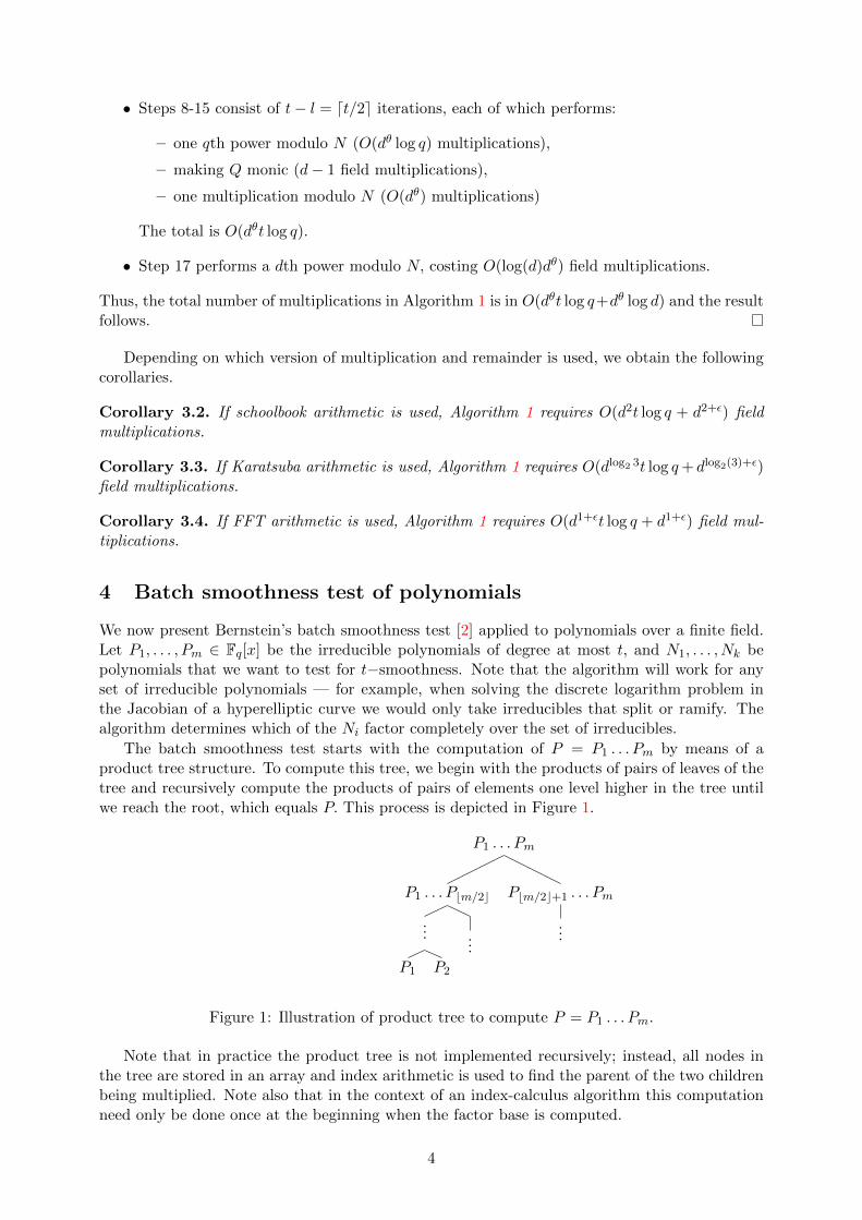
The batch smoothness test starts with the computation of P = P1 . . . Pm by means of aproduct tree structure. To compute this tree, we begin with the products of pairs of leaves of thetree and recursively compute the products of pairs of elements one level higher in the tree untilwe reach the root, which equals P. This process is depicted in Figure 1.

P1 . . . Pm

P1 . . . Pbm/2c

...

P1 P2

...

Pbm/2c+1 . . . Pm

...

Figure 1: Illustration of product tree to compute P = P1 . . . Pm.

Note that in practice the product tree is not implemented recursively; instead, all nodes inthe tree are stored in an array and index arithmetic is used to find the parent of the two childrenbeing multiplied. Note also that in the context of an index-calculus algorithm this computationneed only be done once at the beginning when the factor base is computed.

4

Given P , we then compute P mod N1, . . . , P mod Nk by computing a remainder tree. Wefirst compute the product tree of N1, . . . , Nk as described above, and replace the root N1 . . . Nk

by P mod N1 . . . Nk, Then, using the fact that

P mod N = (P mod NM) mod N, (1)

for N,M ∈ Fq[x], we recursively replace each node’s children with the value stored in the nodemodulo the value stored in the child. At the end, Equation 1 guarantees that the leaves in thetree will contain P mod Ni for every i ≤ k. This process is illustrated in Figure 2.

P mod N1 . . . Nk

P mod N1 . . . Nbk/2c

...

P mod N1 P mod N2

...

P mod Nbk/2c+1 . . . Nk

...

Figure 2: Illustration of the remainder tree of P and N1, . . . , Nk.

At the end of this process, if a leaf node stores zero, then we know that the original value issmooth with respect to the Pi and square-free. To account for higher multiplicities of the Pi, wecould raise the values of each non-zero leaf node (P mod Ni) to the power of an exponent at leastas large as deg(Ni), as in the algorithm from the previous section. In fact, to really amortize thecost of this operation, it is even better to perform the exponentiation at the root of the remaindertree, where the degree of the polynomials involved is the highest (thus exploiting asymptoticallyfast arithmetic). Therefore, prior to computing the remainder tree, we could update P by

P ← P e mod N1 · · ·Nk,

where e is an exponent at least as large as maxi deg(Ni). This method returns all smooth valueswithout false positive. Based on an idea of Coppersmith [5], we use a variant that avoids theexponentiation, but which can return false positive. It consists of calculating N ′i · P mod Ni ateach non-zero leave to account for multiple roots in Ni. Note that this operation could in fact beperformed on the root, but we expect it to produce too many false positive whithout improvingthe theoretical complexity.

Most index-calculus algorithms make use of “large prime” variants, where terms that arecompletely t-smooth except for a small number of factors of degree less than a given large primebound are also useful. In order to detect such partially-smooth polynomials, we remove all thefactors of degree at most t from Ni by computing Ni/ gcd((P mod Ni)

deg(Ni), Ni). If this quantityhas degree at most our given large prime bound, then we accept Ni as being partially smooth.

This method is summarized in Algorithm 2.

5 Complexity analysis

To compare the computational cost of Algorithm 2 (which tests a batch of polynomials) with thatof Algorithm 1 (which tests one), we provide an analysis of the amortized cost of testing a batchof k polynomials of degree d over Fq. We incorporate the crossover points between schoolbook,Karatsuba, and FFT-based polynomial multiplication in our analysis. Indeed, in practical appli-cations, d is not necessarily very large, so it is interesting to assess how the algorithm performs

5

Algorithm 2 Batch smoothness test

Input: B = {P1, · · · , Pm}, N1, · · · , Nk, large prime bound tlp (no large primes if tlp = 0).Output: List L of B-smooth Ni.1: Compute P = P1 . . . Pm using a product tree.2: Compute P mod N1, . . . , P mod Nk using a remainder tree.3: L = {}.4: for i = 1 to k do5: yi = P mod Ni, yi ← N ′i · yi mod Ni.6: if yi = 0 or (tlp > 0 and deg(Ni/ gcd(yi, Ni)) ≤ tlp) then7: L← L ∪ {Ni}.8: end if9: end for

10: return L

in this setting. Let d0 the degree for which Karatsuba multiplication becomes faster than theschoolbook one and d1 the crossover point between FFT and Karatsuba. The crossover pointscan be observed experimentally, as shown in Section 6.

5.1 Cost of the product tree

The cost of the batch smoothness test is amortized, which means that if we test a batch of kpolynomials, we divide the total cost by k.

Theorem 5.1. The amortized cost of calculating the product tree of a batch of k polynomials ofdegree d over Fq is in

O

(d

(d0 + d

log2(3)−11 − dlog2(3)−10 +

(kd)ε − dε12ε − 1

)).

Proof. We begin by analyzing the cost of the steps using “schoolbook” multiplication. We denoteby i ≥ 1 the level of the product tree we are calculating, where i = 1 corresponds to the leaves.At each level, we perform k

2imultiplications between polynomials of degree 2i−1d. We switch to

Karatsuba when 2id = d0, that is when i = i0 := log(⌈

d0d

⌉). The cost of the computation of a

level i ≤ i0 of the product tree is in

O

(k

2i(2id)2) ⊆ O (k2id2

).

The combined cost of all these levels is in

O

kd2 log(⌈

d0d

⌉)∑i=1

2i

⊆ O(kd22log(⌈ d0d ⌉)) ⊆ O(kdd0).

When i0 ≤ i < i1 := log(⌈

d1d

⌉), we use Karatsuba multiplication, and the cost of a level of

the tree is in

O

(k

2i(2id)θ) ⊆ O(kdθ (2θ−1

)i),

where θ = log2(3). The combined cost of all these level is in

O

kdθ

log(⌈

d1d

⌉)∑i=log

(⌈d0d

⌉)(

2θ−1)i

⊆ O(kd

(dθ−11 − dθ−10

2θ−1 − 1

))

6

When i ≥ i1, we use FFT multiplication and the cost of computing one level of the producttree is in

O

(k

2i(2id)θ) ⊆ O(kdθ (2θ−1

)i),

where θ = 1 + ε. The combined cost of all these level is in

O

kdθ log(k)∑i=log

(⌈d1d

⌉)(

2θ−1)i

⊆ O(kd

((kd)θ−1 − dθ−11

2θ−1 − 1

))

The result follows by adding the cost of the computation of the levels i ≤ i0, i0 < i ≤ i1 andi ≥ i1 and dividing by k to get the amortized cost.

As this occurs in particular for polynomials in F2e [X], it is interesting to consider the casewhere no implementation of the FFT multiplication is available.

Corollary 5.2. With the notations of Theorem 5.1, the amortized cost of calculating the prod-uct tree of a batch of k polynomials of degree d over Fq with only schoolbook and Karatsubamultiplication is in

O(d(d0 + (kd)log2(3)−1 − dlog2(3)−10

)).

Proof. The proof immediately follows from that of Theorem 5.1. It suffices to remove the levelsi0 < i ≤ i1.

5.2 Cost of the remainder tree

At the level i < log(k) of the remainder tree, we reduce k2i

degree 2id polynomials modulo 2i−1d

polynomials. As stated in Section 2, this has the same cost as performing k2i

multiplicationsbetween degree-2i−1d polynomials. The computation of the root of the remainder tree (whichcomes first), consists of the reduction of P = P1 · · ·Pm modulo N1 · · ·Nk. Since the cost of theproduct tree and remainder tree increases with k, we only consider the case deg(P ) ≥ kd, as anyother batch size would not be optimal. Then the amortized cost of the computation of the rootof the remainder tree is in

O

(deg(P )θ

k

),

where θ = 1 + ε if FFT multiplication is available, and θ = log2(3) otherwise. The total costof the remaining levels is the same as that of the product tree. The last operation consists of kmultiplications N ′i · P mod Ni between degree d polynomials. Depending on the size of d, this isin the same complexity class as the levels of the product tree using either plain multiplication,Karatsuba, or FFT. It therefore does not appear as an extra term in the overall complexity.

Theorem 5.3. The amortized cost of calculating the remainder tree of a batch of k polynomialsof degree d over Fq is in

O

(deg(P )1+ε

k+ d

(d0 + d

log2(3)−11 − dlog2(3)−10 +

(kd)ε − dε12ε − 1

)).

As previously, we can easily derive an analogue when only schoolbook and Karatsuba multi-plication are available.

Corollary 5.4. If only schoolbook and Karatsuba multiplications are used, the amortized cost ofcalculating the remainder tree of a batch of k polynomials of degree d over Fq is in

O

(deg(P )log2(3)

k+ d

(d0 + (kd)log2(3)−1 − dlog2(3)−10

)).

7

5.3 Optimal size of batch

Let us find the optimal value of k. Whether we use FFT or not, the cost function has the shape

c(k) = A/k +Bkθ−1 + C,

where A = deg(P )θ, B = dθ

2θ−1−1 , C does not depends on k and θ = 1 + ε if we use FFTmultiplication, θ = log2(3) otherwise. A critical point for this function is attained for

kopt =

(A

(θ − 1)B

)1/θ

∈ O(

deg(P )

d

).

5.4 Overall cost

By combining the optimmal size of batch with the expression of the cost of the remainder treeas a function of k, we naturally get the overall cost.

Theorem 5.5. The amortized cost of Algorithm 2 is given by

O

(ddeg(P )ε + d

(d0 + d

log2(3)−11 − dlog2(3)−10 +

(deg(P ))ε − dε12ε − 1

))when FFT multiplication is available.

Corollary 5.6. If only schoolbook and Karatsuba multiplications are used, the amortized cost ofAlgorithm 2 is in

O(ddeg(P )log2(3)−1 + d

(d0 − dlog2(3)−10

)).

Thus, as a function of d,, the batch algorithm has roughly the same asymptotic complexity asthe single polynomial test. We also see that for d ≤ d0, where the single polynomial test uses onlyschoolbook arithmetic but the batch algorithm may use Karatsuba or FFT, the batch algorithmis also not expected to offer much improvment. In particular, the costs given in Theorem 5.5and its corollary both have a term of the form dd0 which, for d close to d0 is d2. Although someof this is cancelled by negative terms in the cost functions, we still expect the overall cost to becloser to d2. The situation is similar for values of d close to the FFT threshold d1.

The dependency in t (where t is the bound on the degree of the factor base elements) ishidden in the term in deg(P ). Asymptotically, as q → ∞, we have deg(P ) ∈ O(qt). WhenAlgorithm 2 is used with FFT multiplication, we have a term in deg(P )ε. Here, the ε representsthe logarithmic terms in the FFT complexity, so deg(P )ε is roughly O(log(qt) log log(qt)), whichis O(t log t) as t goes to infinity. Therefore, the dependence on t in Algorithm 2 is super-linearwhen FFT multiplication is used, as opposed to linear for Algorithm 1. On the other hand, ifonly Karatsuba multiplication is used, then large values of t will have a considerable impact onthe performances of Algorithm 2 since the dependency in t is exponential.

6 Computational results

Although our analysis predicts that the batch smoothness test and the single tests will havesimilar performances as d → ∞, it is expected to be somewhat more complicated in practice.First, our asymptotic analysis suppressed logarithmic terms and constants and hence does notadequately differentiate between the actual costs of multiplication and remainder computation.Thus, the actual runtime functions are more complicated, as well as our estimate of an optimalbatch size. Secondly, implementations of polynomial arithmetic generally use more algorithmsthan the two assumed in our analysis. As a minimum, Karatsuba multiplication is used for somerange of polynomial degrees between “schoolbook” and FFT algorithms (eg. NTL [13] switchesto Karatsuba for degree greater than 16)) and some switch between other algorithms as well (eg.the GF2X library [1]). In this section, we give numerical data comparing the performance of thesingle-polynomial and batch smoothness tests.

8

6.1 Arithmetic operations

The crossover points d0 between “schoolbook” and Karatsuba multiplication, and d1 betweenKaratsuba and FFT multiplication, occur in the analysis of the batch smoothness test describedin Section 5. It is interesting to know if these only have a theoretical significance or if they occurin the practical experiments that we ran. To illustrate that this is the case, we show the evolutionof the run time of multiplication and division as d grows in F31[x] and F2[x]. Table 1 comparesthe quadratic time multiplication and division (respectively denotes as Plain mul and Plain rem)to the quasi-linear time method based on FFT for polynomials in F31[x] of degree between 100and 90000. The implementation used is the one of the NTL library [13]. In Table 2, we compareToom-Cook multiplication and the FFT-based multiplication for polynomials of degree between150000 and 100000000 with the gf2x library [1]. In both cases, the timings in CPU msec for 100operations were obtained on an Intel Xeon 1.87 GHz with 256 GB of memory and are presentedin the Appendix. The crossover point for polynomials in F31[x] is around d = 400 and ford = 150000 in F2[x]. Note that strictly speaking, these timings do not give the value of d1.Indeed, we could not isolate Karatsuba multiplication in the corresponding libraries. Also, wecould not run the FFT-based algorithm using F2[x] for d < 150000 because the thresholds werehard coded. However, we can certainly hope from the timings that d1 (and thus d0) are withinpractical reach.

6.2 Optimal size of batch

The analysis of the batch smoothness test in Section 5 showed the existence of an optimal size

of batch k of the form kopt = O(deg(P )d

). To illustrate the impact of k on the run time, we

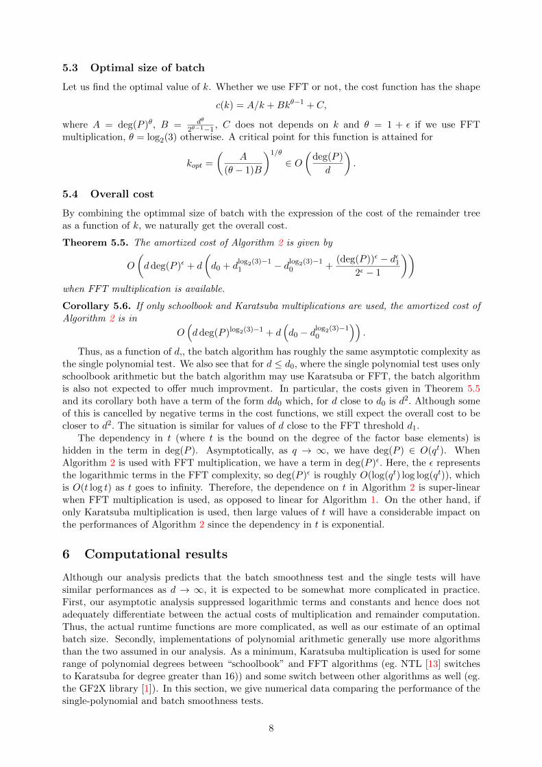
fixed d = 100 and tested the t-smoothness of 100 polynomials in F2[x] for t = 25. We ran ourexperiment on an Intel Xeon 1.87 GHz with 256 GB of memory. The corresponding timingsare presented in the Appendix. Figure 3 shows the graph of the amortized time in CPU msecfor log(k) = 5, · · · , 19. Note that we only take powers of 2 to optimize the use of the treestructure. We clearly see that there is an optimum value. On the same architecture, we ran otherexperiments to show the dependency of the optimal value of k on d and deg(P ). Table 3 showsthe optimal value of k for the test of smoothness of polynomials in F2[x] of fixed degree d = 100when t varies between 5 and 25. Likewise, in Table 4, we fix t = 25 and let the degree of thepolynomials in F2[x] vary between 100 and 1000. In each case, the metric to choose the optimalk is the amortized CPU time for 100 tests. Despite a few outliers, the general trend predictedby the theory seems to be respected. Table 3 shows that the optimal value of k gets larger as t(and thus deg(P )) gets larger. Meanwhile, Table 4 shows that when d gets larger, the optimal kgets smaller, which is consistent with the term in 1

d predicted by the analysis. Since the analysisof Section 5 is asymptotic, and since only moderate values of d and t are within practical range,it is delicate to confirm the theory with our available data. In addition, we have a very lowgranularity for k (20 different values). However, the results presented in Table 3 and 4 are quitepromising. Indeed, we can see for example that in Table 3 for deg(P ) = 67100116, k = 131072while for deg(P ) = 8384230, k = 16384. As 67100116

8384230 ≈ 8 = 13107216384 , this is consistent with a linear

dependence in deg(P ). In Table 4, we have k = 131072 for g = 100 while k = 16384 for g = 1000.We have 131072

16384 = 8 while the dependency in 1d predicted by the analysis suggests a ratio of 10.

6.3 Dependence on t

The smoothness test algorithms presented in Section 3 and Section 4 both depend on the bound ton the degree of the polynomials in the factor base. The larger t, the more expensive a smoothnesstest is. The expected time of Algorithm 1 has a term in tdθ log(q) where 1 < θ ≤ 2. As discussedin the previous section, the dependence on t in the cost of Algorithm 2 is expected to be roughlyt log t when FFT multiplication is used.

9

Figure 3: Optimal value of k in F2[x] for t = 25 and d = 100

0

2

4

6

8

10

12

14

16

8 10 12 14 16 18

Tim

e

log(k)

To illustrate this, we ran experiments in F2[x] and F3[x] to show the impact of FFT multipli-cation, and in F4[x] where we only have “schoolbook” and Karatsuba multiplication. We fixedthe degree d of the polynomials to be tested to d = 200 in F2[x] and F3[x], and d = 10 in F4[x].We measured the time to test the t-smoothness of 100 polynomials for t between 5 and 25 inF2[x], between 5 and 15 in F3[x] and between 5 and 10 in F4[x]. In each case, we compare theamortized cost of testing the smoothness of one polynomial using Algorithm 1 (single FFT forF2[x] and F3[x], single Karatsuba for F4[x]) and Algorithm 2 (batch test). The timings, which aredisplayed in Table 5 Table 6, and Table 7 available in the Appendix were obtained on a machinewith 64 Intel Xeon X7560 2.27 GHz cores and 256 GB of shared RAM.

Figure 4: Dependency on t in F2[x] with d = 200

0

0.05

0.1

0.15

0.2

0.25

0.3

0.35

0.4

5 10 15 20 25

tim

e (m

s)

t

Comparison over GF(2) with d=200

Single testBatch test

All the timings show that the cost increases with the size of t. The analysis predicts a lineardependency in t for the single tests. We see in Table 5 that this is consistent with the timings ofAlgorithm 1 with FFT. For example, in F2[x] for t = 25, the average time is 0.0957 msec whileit is 0.0255 for t = 5. We have 0.0957

0.0255 ≈ 3.75 while the theory predicts a ratio of 5. Likewise, inF3[x], the time for t = 15 is 5.263 msec while it is 1.597 for t = 5, which is a ratio of 5.263

1.597 ≈ 3.29while the theory predicts a ratio of 3. The expected super-linear dependency in t of Algorithm 2

10

with FFT multiplication does not appear quite as clearly, but the growth does appear to be worsethan linear.

Table 7 shows us the dependency in t for Algorithm 1 and Algorithm 2 in F4[x]. The timefor Algorithm 1 with t = 10 is 2.437 while it is 1.396 for t = 5. The ratio is 2.437

1.396 ≈ 1.74 whilethe theory predicts a ratio of 2. For Algorithm 2, the time with t = 10 is 3.867 while it is 1.428for t = 5. The ratio is 3.867

1.428 ≈ 2.70. In this case, NTL uses Kronecker substitution to performthe multiplication in F2[x] using asymptotically fast arithmetic, so the expected ratio should beslightly above 2.

6.4 Dependency in d

When fast multiplication is assumed, the asymptotic complexity of both Algorithm 1 and Algo-rithm 2 is quasi linear in d, and when using Karatsuba multiplication, the theory predicts thatit is in dlog2(3). To illustrate this, we ran experiments for fixed values of t and increasing d inF2[x], F3[x] and F4[x]. We compared the performances of the single test with FFT multiplication(single FFT) and Algorithm 2 (batch test). In F4[x], only Karatsuba multiplication is availablefor both Algorithm 1 (denoted single Karatsuba) and for Algorithm 2. The timings, which aredisplayed in Table 8, Table 9, Table 10, and Table 11 available in the Appendix were obtainedon a machine with 64 Intel Xeon X7560 2.27 GHz cores and 256 GB of shared RAM.

Figure 5: Dependency on d for large d in F2[x] for t = 20

0

200

400

600

800

1000

1200

1400

1600

1800

0 100000 200000 300000 400000 500000 600000 700000 800000 900000 1e+06

tim

e (m

s)

d

Comparison over GF(2) with t=20

single FFTbatch test

We observe that Algorithm 1 and Algorithm 2 perform very similarly when using either theFFT multiplication. In addition, according to the theory, their run time seems to grow linearlywith the degree once d is sufficiently large. This is shown in particular in Figure 5, in the caseof F2[x] where FFT arithmetic is available and we consider d up to 106. Our experiments forF4 presented in Figure 7 also show a roughly linear growth. Note that these experiments weredesigned to investigate the performance of the algorithm for values of d close to d0, the Karatsubathreshold. For larger values of d, NTL switches to Kronecker substitution, using the quasi-linearFFT implementation of GF2X.

The linearity in d is less clear for d ≤ 1000 as shown in Figure 6 in F2[x] for t = 10. However,it is interesting to note that the variations of the cost with Algorithm 1 and Algorithm 2 are verysimilar. This similarity is also well illustrated by Figure 7 which shows the dependency on d inthe run time of Algorithm 1 and Algorithm 2 for d ≤ 100 in F4[x] for t = 6. Once d > 25, thecost functions seem to differ by a constant, as predicted by the theory.

11

Figure 6: Dependency on d for small d in F2[x] for t = 10

0

0.02

0.04

0.06

0.08

0.1

0.12

0 100 200 300 400 500 600 700 800 900 1000

tim

e (m

s)

d

Comparison over GF(2) with t=10 and small d

Single testBatch test

Figure 7: Dependency on d for small d in F4[x] for t = 6

0

0.2

0.4

0.6

0.8

1

1.2

1.4

0 10 20 30 40 50 60 70 80 90 100

tim

e (m

s)

d

Comparison over GF(4) with t=6

Single test (Karatsuba)Batch test

For small values of d near the thresholds d0 and d1, we also see both algorithms exhibitingroughly the same performance. Recall that one motivation for considering the batch algorithmin this context is that it can take advantage of asymptotically faster arithmetic in cases whenthe single polynomial algorithm is forced to use schoolbook arithmetic. Unfortunately we didnot observe a dramatic improvement even in this scenario. For example, in Figure 7 (F4[x]) wenotice that the two algorithms have roughly the same performance when d is close to 16, NTL’sthreshold for swithching from schoolbook arithmetic to Karatsuba in this case.

In all our timings showing the dependency in d for fixed t, Algorithm 1 performs better (bya constant factor) than Algorithm 2 at the notable exception of Table 10 which shows the runtime in F3[x] for fixed t = 5. There, the batch smoothness test seems to provide a mild speed-upby a constant factor. This may be explained by the conjunction of a small value of t (and thus

12

of deg(P )) and by lower thresholds for the value of d1 where the fast multiplication becomescompetitive (which occurs in the theoretical prediction).

6.5 Examples of practical relevance

Our first example is the curve C155 from [14], a genus 31 hyperelliptic curve defined over F25 .This curve is the result of the Weil descent on an elliptic curve over F2155 as shown in [8]. Forthis example, a smoothness bound of 4 is used and the polynomials to be factored have degree36. The optimal size of batch is k = 32768. The average times for testing the smoothness ofdegree-36 polynomials are

• 0.0005884 CPU sec with single test and fast multiplication,

• 0.0012091 CPU sec with the batch test.

The timings were obtained on a machine with 64 Intel Xeon X7560 2.27 GHz cores and 256GB of shared RAM. The implementation of polynomial arithmetic in F25 [X] we used only hasschool-book and Karatsuba remainder algorithms available (no FFT) — we expect somewhatbetter performance of the batch method if FFT were added to the implementation.

Our second example is taken from the discrete logarithm computation in F21039 describedin [6]. Here, we assume a smoothness bound of 25 and that the polynomials in F2[x] in thecofactorization step have degree 99. The factor base has 2807196 primes and the degree of theirproduct is 67100116. The optimal batch size is k = 131072. The average times for testing thesmoothness of degree-99 polynomials are

• 0.00007016 CPU sec with single test and fast multiplication,

• 0.00019327 CPU sec with the batch test.

The timings were obtained on a machine with 64 Intel Xeon X7560 2.27 GHz cores and 256 GBof shared RAM. This computation makes use of the GF2X library directly, which does includeoptimized polynomial arithmetic for large degree operands.

7 Conclusion

Our theoretical analysis and numerical experiments show that the batch smoothness test doesin general not out-perform the simpler, more memory-friendly single polynomial test. The the-oretical analysis shows that if FFT multiplication is available, both methods have the sameasymptotic quasi-linear complexity with respect to the degree d of the polynomials to be tested.As a function of the smoothness bound, the batch method has worse asymptotic complexity,namely super-linear as opposed to linear. In most practical cases, for sufficiently large d thebehavior of the two methods only differs by a constant, thus backing up the theory. The singlesmoothness test is more efficient in almost all cases. The two factors that can make the batchsmoothness test faster than single tests are a low smoothness bound and a low threshold on thedegree for which FFT multiplication becomes fast, as we can see in Table 10.

References

[1] gf2x, a C/C++ software package containing routines for fast arithmetic in GF(2)[x] (mul-tiplication, squaring, GCD) and searching for irreducible/primitive trinomials. Available athttp://gf2x.gforge.inria.fr/.

[2] D. Bernstein, How to find smooth parts of integers, submited to Mathematics of Computation.

13

[3] J.-F. Biasse and M. Jacobson, Practical improvements to class group and regulator com-putation of real quadratic fields, Algorithmic Number Theory - ANTS-IX (Nancy, France)(G. Hanrot, F. Morain, and E. Thome, eds.), Lecture Notes in Computer Science, vol. 6197,Springer-Verlag, 2010, pp. 50–65.

[4] G. Bisson and A. Sutherland, Computing the endomorphism ring of an ordinary ellipticcurve over a finite field, Journal of Number Theory 113 (2011), 815–831.

[5] D. Coppersmith, Fast evaluation of logarithms in fields of characteristic two, IEEE Trans-actions on Information Theory 30 (1984), no. 4, 587–594.

[6] J. Detrey, P. Gaudry, and M. Videau, Relation collection for the function field sieve, ARITH21 - 21st IEEE International Symposium on Computer Arithmetic (Austin, Texas, UnitedStates) (A. Nannarelli, P.-M. Seidel, and P. Tang, eds.), IEEE, 2013, pp. 201–210.

[7] A. Enge and P. Gaudry, A general framework for subexponential discrete logarithm algo-rithms, Acta Arithmetica 102 (2002), 83–103.

[8] M. Jacobson, A. Menezes, and A. Stein, Solving elliptic curve discrete logarithm problemsusing weil descent, Journal of the Ramanujan Mathematical Society 16 (2001), 231–260.

[9] H. Lenstra, Factoring integers with elliptic curves, The Annals of Mathematics 126 (1987),no. 3, 649–673.

[10] R. Lidl and H. Niederreiter, Introduction to finite fields and their applications, CambridgeUniversity Press, New York, NY, USA, 1986.

[11] A. Odlyzko, Discrete logarithms in finite fields and their cryptographic significance, Proc.Of the EUROCRYPT 84 Workshop on Advances in Cryptology: Theory and Applicationof Cryptographic Techniques (New York, NY, USA), Springer-Verlag New York, Inc., 1985,pp. 224–314.

[12] A. Schnhage and V. Strassen, Schnelle multiplikation groer zahlen, Computing 7 (1971),no. 3-4, 281–292 (German).

[13] V. Shoup, NTL: A Library for doing Number Theory, Software, 2010, http://www.shoup.net/ntl.

[14] M. Velichka, M. Jacobson, and A. Stein, Computing discrete logarithms in the jacobianof high-genus hyperelliptic curves over even characteristic finite fields, 2013, To appear inMathematics of Computation.

14

A Timings

In this appendix, we present the timings that were used to illustrate the theoretical predictions onthe run time of Algorithm 1 and Algorithm 2, as well as for the comparison of their performance.Table 1, Table 2, Table 3 and Table 4 were obtained on an Intel Xeon 1.87 GHz with 256 GB ofmemory while the rest of the timings was obtained on a machine with 64 Intel Xeon X7560 2.27GHz cores and 256 GB of shared RAM.

Table 1: Arithmetic operations in F31 with respect to the degree d

d Plain mul FFT mul Plain rem FFT rem

100 10 30 30 60200 40 50 120 160300 70 100 280 330400 110 100 490 340500 160 110 760 360600 230 200 1100 710700 270 200 1500 720800 340 210 1940 730900 400 220 2480 750

1000 480 220 3060 7602000 1470 470 12200 16203000 2760 920 26690 33204000 4340 980 47570 34505000 6610 1860 74160 68806000 8210 1920 109350 72607000 10340 2000 149180 73708000 13130 2050 195620 74809000 16820 3920 246860 14870

10000 19900 3900 304000 1520020000 59800 8400 1176800 3080030000 100200 8700 2606200 2740040000 178900 17400 4713200 5620050000 244600 18400 7702100 6620060000 302700 18500 10073400 5760070000 431900 34800 14829300 13410080000 532000 35700 19094700 13790090000 600400 37100 24063600 141400

15

Table 2: Multiplication in F2[x] with respect to the degree d

d Toom-Cook mul FFT mul

150000 470 430250000 950 690500000 2430 1490

1000000 6650 32505000000 63840 23200

10000000 183330 5503050000000 1595270 314470

100000000 4110380 731010

Table 3: Influence of t on the optimal value of k for d = 100

t deg(P ) k

5 52 10246 106 10247 232 10248 472 10249 976 1024

10 1966 102411 4012 204812 8032 102413 16222 204814 32476 409615 65206 102416 130486 204817 261556 204818 523132 409619 1047418 819220 2094958 1638421 4191976 3276822 8384230 1638423 16772836 13107224 33545716 26214425 67100116 131072

16

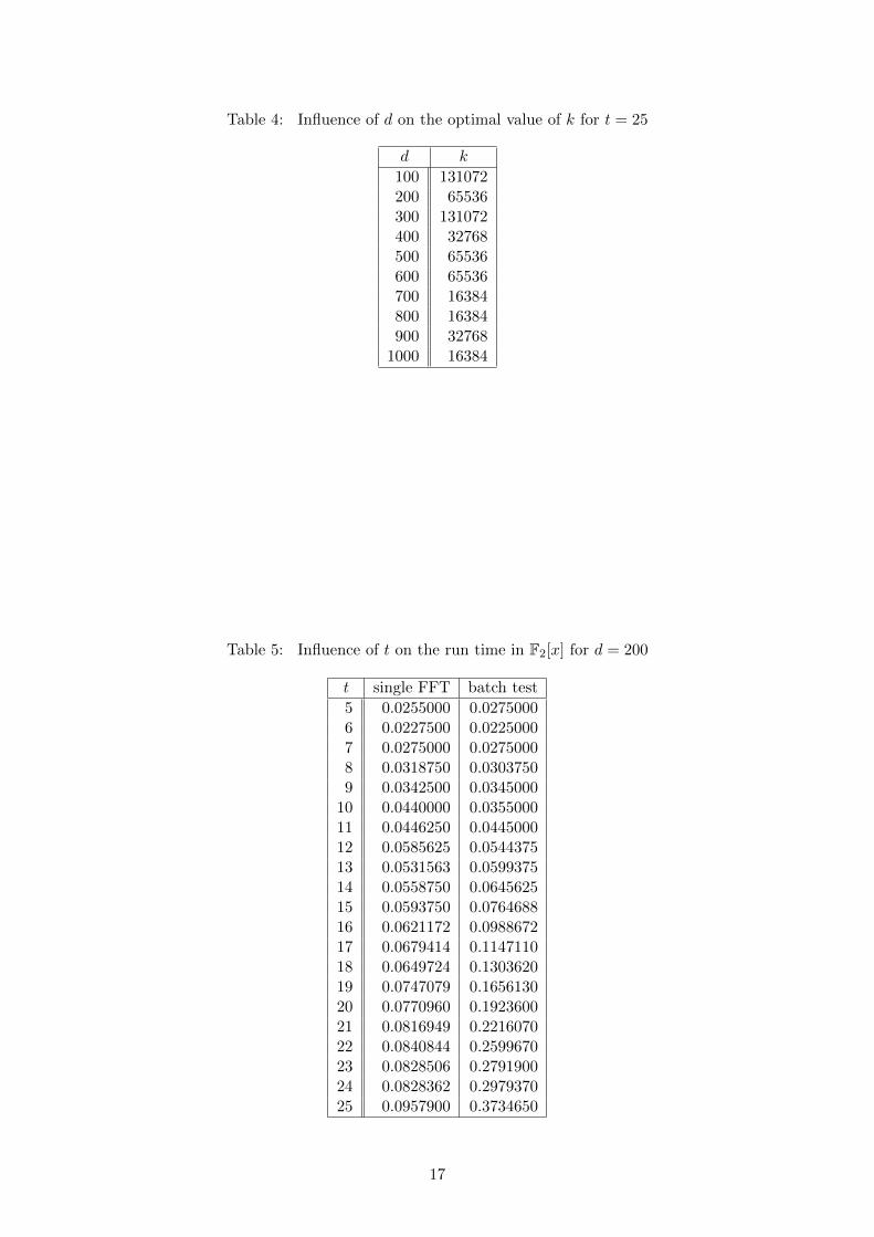
Table 4: Influence of d on the optimal value of k for t = 25

d k

100 131072200 65536300 131072400 32768500 65536600 65536700 16384800 16384900 32768

1000 16384

Table 5: Influence of t on the run time in F2[x] for d = 200

t single FFT batch test

5 0.0255000 0.02750006 0.0227500 0.02250007 0.0275000 0.02750008 0.0318750 0.03037509 0.0342500 0.0345000

10 0.0440000 0.035500011 0.0446250 0.044500012 0.0585625 0.054437513 0.0531563 0.059937514 0.0558750 0.064562515 0.0593750 0.076468816 0.0621172 0.098867217 0.0679414 0.114711018 0.0649724 0.130362019 0.0747079 0.165613020 0.0770960 0.192360021 0.0816949 0.221607022 0.0840844 0.259967023 0.0828506 0.279190024 0.0828362 0.297937025 0.0957900 0.3734650

17

Table 6: Influence of t on the run time in F3[x] for d = 200

t single FFT batch test

5 1.59750 1.511506 1.99750 2.024507 2.41375 2.437508 2.52275 2.859629 3.19660 3.82236

10 3.44301 4.4703311 3.82687 5.3938512 4.00995 6.0748213 4.56101 7.2581814 4.84185 8.5321715 5.26337 11.35560

Table 7: Influence of t on the run time in F4[x] for d = 10

t single Karatsuba batch test

5 1.39675 1.428756 1.63213 1.806317 1.92971 2.212728 2.11232 2.680869 2.40723 3.20971

10 2.43713 3.86726

18

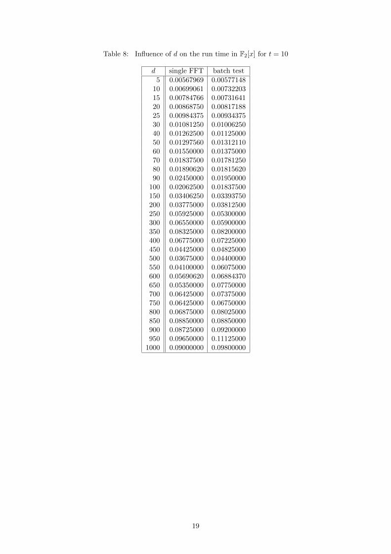
Table 8: Influence of d on the run time in F2[x] for t = 10

d single FFT batch test

5 0.00567969 0.0057714810 0.00699061 0.0073220315 0.00784766 0.0073164120 0.00868750 0.0081718825 0.00984375 0.0093437530 0.01081250 0.0100625040 0.01262500 0.0112500050 0.01297560 0.0131211060 0.01550000 0.0137500070 0.01837500 0.0178125080 0.01890620 0.0181562090 0.02450000 0.01950000

100 0.02062500 0.01837500150 0.03406250 0.03393750200 0.03775000 0.03812500250 0.05925000 0.05300000300 0.06550000 0.05900000350 0.08325000 0.08200000400 0.06775000 0.07225000450 0.04425000 0.04825000500 0.03675000 0.04400000550 0.04100000 0.06075000600 0.05690620 0.06884370650 0.05350000 0.07750000700 0.06425000 0.07375000750 0.06425000 0.06750000800 0.06875000 0.08025000850 0.08850000 0.08850000900 0.08725000 0.09200000950 0.09650000 0.11125000

1000 0.09000000 0.09800000

19

Table 9: Influence of large d on the run time in F2[x] for t = 20

d single FFT batch test

1000 0.16896600 0.809267001500 0.34201700 1.322100002000 0.43851000 1.719190002500 0.65992600 2.076960003000 0.99763800 2.735190004000 1.33407000 3.304580005000 1.91657000 4.233400006000 2.71314000 5.716780007000 3.26151000 6.245010008000 3.85816000 7.042510009000 4.83971000 8.08675000

10000 6.14594000 9.6503600050000 50.58590000 58.94140000

100000 134.76200000 140.34500000

Table 10: Influence of d on the run time in F3[x] for t = 5

d single FFT batch test

5 0.00948437 0.014781210 0.02300000 0.026750015 0.03675000 0.042750020 0.05100000 0.057250025 0.07250000 0.080750030 0.10275000 0.111250040 0.14700000 0.147250050 0.31050000 0.276750060 0.37475000 0.343500070 0.60350000 0.516250080 0.59375000 0.526750090 0.70975000 0.6420000

100 0.64875000 0.6045000150 1.24425000 1.1432500200 1.34800000 1.2955000250 2.03675000 1.9017500300 3.50200000 3.1397500350 3.88800000 3.6395000400 3.51150000 3.2830000450 3.76100000 3.4872500500 4.28825000 4.0065000550 7.23575000 6.8602500600 7.38875000 7.0150000650 7.47050000 6.8910000

20

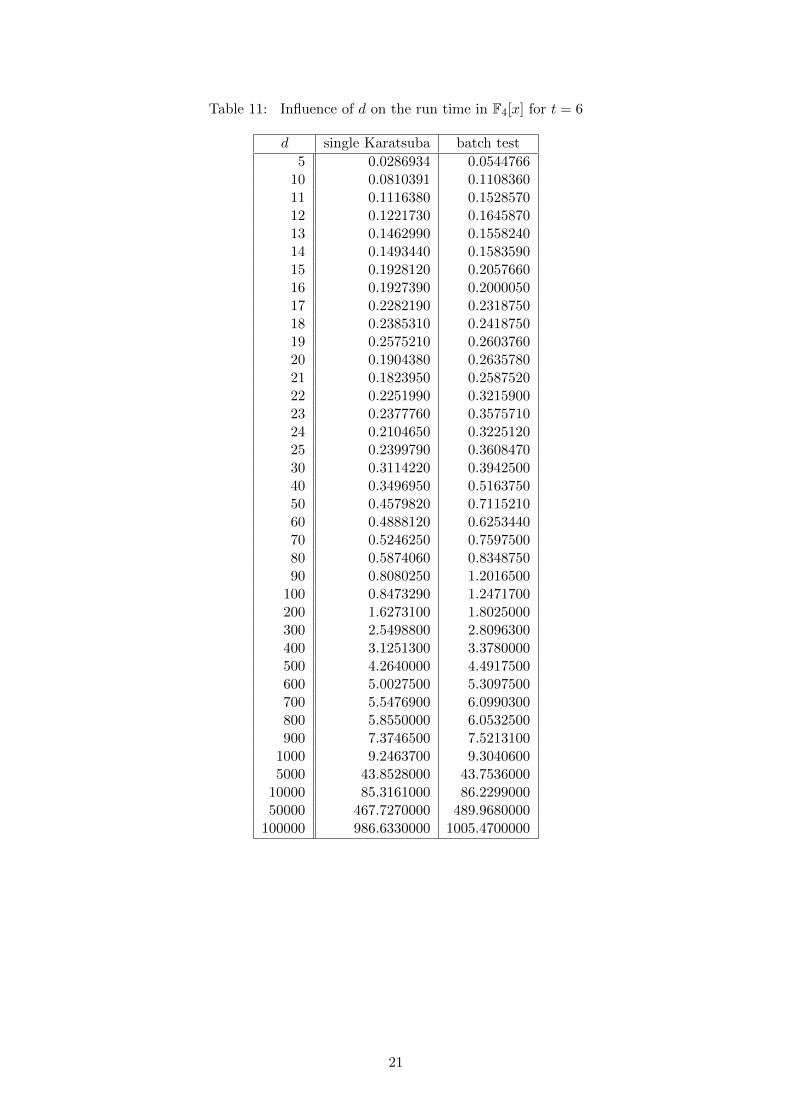
Table 11: Influence of d on the run time in F4[x] for t = 6

d single Karatsuba batch test

5 0.0286934 0.054476610 0.0810391 0.110836011 0.1116380 0.152857012 0.1221730 0.164587013 0.1462990 0.155824014 0.1493440 0.158359015 0.1928120 0.205766016 0.1927390 0.200005017 0.2282190 0.231875018 0.2385310 0.241875019 0.2575210 0.260376020 0.1904380 0.263578021 0.1823950 0.258752022 0.2251990 0.321590023 0.2377760 0.357571024 0.2104650 0.322512025 0.2399790 0.360847030 0.3114220 0.394250040 0.3496950 0.516375050 0.4579820 0.711521060 0.4888120 0.625344070 0.5246250 0.759750080 0.5874060 0.834875090 0.8080250 1.2016500

100 0.8473290 1.2471700200 1.6273100 1.8025000300 2.5498800 2.8096300400 3.1251300 3.3780000500 4.2640000 4.4917500600 5.0027500 5.3097500700 5.5476900 6.0990300800 5.8550000 6.0532500900 7.3746500 7.5213100

1000 9.2463700 9.30406005000 43.8528000 43.7536000

10000 85.3161000 86.229900050000 467.7270000 489.9680000

100000 986.6330000 1005.4700000

21