SNPs2ChIP: Latent Factors of ChIP-seq to infer functions ...psb.stanford.edu/psb-online/proceedings/psb19/anand.pdf · To normalize batch e ects in each ChIP-map, we applied the SVA

SNPs2ChIP: Latent Factors of ChIP-seq to infer functions of non-coding SNPs

Shankara Anand*, Laurynas Kalesinskas*, Craig Smail*, and Yosuke Tanigawa*†

Department of Biomedical Data Science, Stanford University, Stanford, CA 94305, U.S.A.*These authors contributed equally to this work.

†E-mail: [email protected]

Genetic variations of the human genome are linked to many disease phenotypes. Whilewhole-genome sequencing and genome-wide association studies (GWAS) have uncovered anumber of genotype-phenotype associations, their functional interpretation remains chal-lenging given most single nucleotide polymorphisms (SNPs) fall into the non-coding regionof the genome. Advances in chromatin immunoprecipitation sequencing (ChIP-seq) havemade large-scale repositories of epigenetic data available, allowing investigation of coordi-nated mechanisms of epigenetic markers and transcriptional regulation and their influenceon biological functions. To address this, we propose SNPs2ChIP, a method to infer bio-logical functions of non-coding variants through unsupervised statistical learning methodsapplied to publicly-available epigenetic datasets. We systematically characterized latent fac-tors by applying singular value decomposition to 652 ChIP-seq tracks of lymphoblastoid celllines, and annotated the biological function of each latent factor using the genomic regionenrichment analysis tool. Using these annotated latent factors as reference, we developedSNPs2ChIP, a pipeline that takes genomic region(s) as an input, identifies the relevant latentfactors with quantitative scores, and returns them along with their inferred functions. Asa case study, we focused on systemic lupus erythematosus and demonstrated our method’sability to infer relevant biological functions. We systematically applied SNPs2ChIP on pub-licly available datasets, including known GWAS associations from the GWAS catalogue andChIP-seq peaks from a previously published study. Our approach to leverage latent patternsacross genome-wide epigenetic datasets to infer the biological functions will advance under-standing of the genetics of human diseases by accelerating the interpretation of non-codinggenomes.

Keywords: non-coding genome; functional interpretation; epigenome; latent factor discovery;biomedical ontology; enrichment analysis; large-scale inference; data integration

1. Introduction

Genome-wide association studies (GWAS) have successfully identified many associations be-tween genetic variants and human diseases.1,2 However, functional interpretation of these as-sociations remains challenging as most GWAS hits fall into non-coding regions of the genome.3

Advancements in high-throughput genome-wide molecular profiling methods, such as ChIP-seq, enable molecular characterization of gene regulatory landscapes, such as histone modifica-tion and transcription factor (TF) binding profiles.4 Leveraging growing biomedical ontologies,such as the gene ontology (GO), human phenotype ontology (HPO), and Mouse Genome Infor-

c© 2018 The Authors. Open Access chapter published by World Scientific Publishing Company anddistributed under the terms of the Creative Commons Attribution Non-Commercial (CC BY-NC)4.0 License.

Pacific Symposium on Biocomputing 2019

184

matics (MGI) phenotype ontology, tools based on statistical enrichment analysis on genomicregions, such as the genomic region enrichment analysis tool (GREAT), have been used toinvestigate the function of the non-coding genome.5–9 Further, collaborative research efforts,such as ENCODE, the Roadmap Epigenomics project, and Genotype-Tissue Expression pro-gram (GTEx), have also systematically generated data-rich molecular catalogues.10–12 Theselarge-scale epigenomic profiles, as well as other publicly available datasets on the NCBI se-quence read archive, are integrated into epigenetic data resources, such as ChIP-Atlas andReMap, which provides an emerging opportunity for data mining and meta-analysis.13,14

Advancements in epigenetic analysis suggest that latent patterns in epigenomic regula-tory profiles can be discovered and characterized for downstream analyses. For example, oneTF can bind to numerous genomic loci with specific sequence features and multiple TFscan work together by forming dimers, executing coordinated transcriptional regulatory pro-grams.15 Moreover, it is known that many TFs have multiple functions through precise co-ordination in different contexts, that there are known interactions between histone modifica-tions and TF occupancy, and that histone modifications and TF occupancy influence geneexpression.10–12,15 With these phenomena in mind, there has been works in harnessing thesepatterns for functional interpretation of non-coding genomes. ChromHMM and Segway, unsu-pervised statistical learning methods, successfully summarizes patterns of epigenetic profilesas interpretable annotations,16,17 while eQTL studies examines non-coding variants in light ofmolecular phenotype, such as expression levels of neighboring genes.12 While these approachesshow some success in utilizing neighboring epigenomic signals to explore molecular interpre-tation of non-coding genomes, they are limited in leveraging genome-wide patterns of bothhistone modification and TF occupancy across different functional contexts. In principle, onecan extend these analyses by leveraging all experimentally collected epigenomic profiles andcharacterizing latent patterns for functional interpretation of non-coding genomic regions ona genome-wide scale.

Here we present SNPs2ChIP, a novel method to infer function of non-coding variants by (1)characterizing latent patterns in epigenomic regulatory profiles using an unsupervised latentfactor discovery algorithm applied to 652 ChIP-seq tracks in the ChIP-Atlas dataset, (2) infer-ring the biological functions of the identified latent factors using GREAT enrichment analysis,and (3) development of a pipeline that takes genomic loci as input and infers functionality ofthe loci by identifying relevant latent factors using a quantitative score. Our computationalapproach contributes to dissecting the genetic architecture of human diseases by acceleratingfunctional interpretation of non-coding variants.

2. Results

2.1. SNPs2ChIP analysis framework overview

We developed a method, SNPs2ChIP, to infer functions of non-coding loci that consists of twocomputational steps: (A) construction of reference ChIP-maps and (B) using the referenceChIP-maps to infer biological functions for user queries. To briefly summarize the first part ofour method, we collected chromatin-profiling data from ChIP-Atlas, one of the largest publicly-available databases of ChIP-seq signals with manually curated metadata,13 and featurized the


185

ChIP-seq peaks(A) Reference dataset construction

1kb

ChI

P-se

q tr

acks

ChIP-map

Genomic bins

Latent factors

Batch normalization (SVA) Latent factor discovery (SVD)

Putative biological functions

Biological characterization

(GREAT)

(B) Inference of biological functions from user’s input query

Query from user:—GWAS SNPs —ChIP-seq peak(s) —Genomic coordinate(s)

Ranked latent factors with biological

annotations

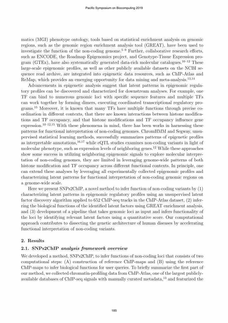
Fig. 1. SNPs2ChIP method overview. (A) Construction of SNPs2ChIP reference dataset. ChIP-seqpeaks of 652 assays are aggregated into a feature matrix, ChIP-map, followed by batch normalizationwith surrogate variable analysis (SVA). Latent factors are characterized with singular value decompo-sition (SVD) and their biological functions are inferred with the genomic region enrichment analysistool (GREAT). (B) SNPs2ChIP pipeline. Using the pre-computed reference, SNPs2ChIP identifiesthe most relevant latent factors and returns them with their annotated biological functions.

ChIP-seq peaks across TFs and histone marks into a matrix, called a “ChIP-map.” To balancethe trade-off in specificity of the functional prediction and the genomic coverage of the ChIP-map, we prepared two matrices for high-specificity and high-coverage analysis, by varying thestringency of the featurization methods. After featurization, we applied batch normalizationwith surrogate variable analysis (SVA) and singular value decomposition (SVD) in each map,resulting latent factors preserving a linear structure optimal for interpretation..18 This wasfollowed by applying GREAT to find the biological functions enriched in each latent factor(Fig. 1A).9 With latent factors and enriched functions as pre-computed reference, we developeda pipeline that takes a loci as input and returns a list of relevant latent factors as well as theirenriched function. A query can be one or multiple genomic loci: GWAS SNPs, ChIP-seq peaks,or genomic coordinates of interest (Fig. 1B).

2.2. Batch normalization of heterogeneous epigenetic features

We focused on 652 lymphoblastoid cell line experiments, the most numerous cell line in theChIP-Atlas database, and downloaded all non-empty ChIP-seq peak files. We divided theentire genome into genomic bins of 1 kbp in size and placed ChIP-seq peaks, represented bythe strength of the peak, into the bins. This was done across 652 tracks, which created a


186

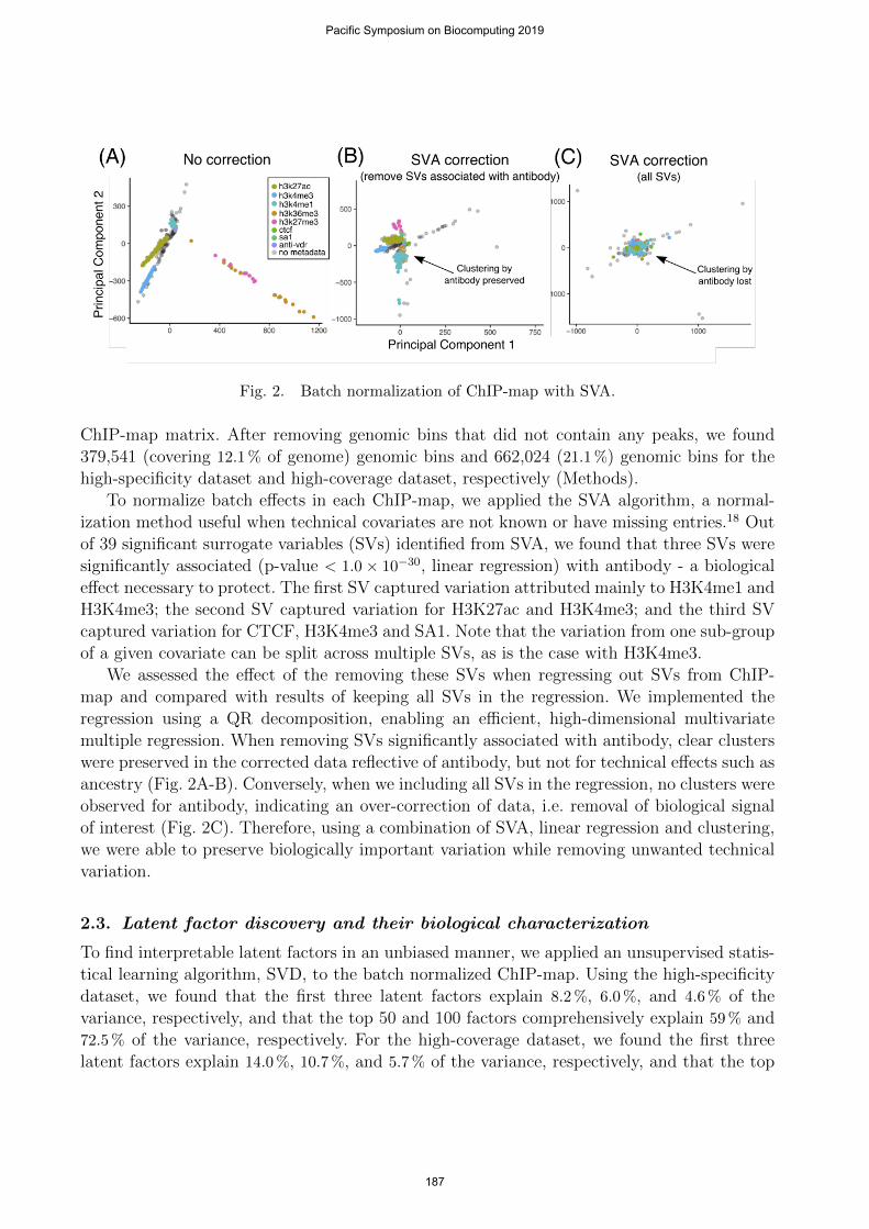
Fig. 2. Batch normalization of ChIP-map with SVA.

ChIP-map matrix. After removing genomic bins that did not contain any peaks, we found379,541 (covering 12.1 % of genome) genomic bins and 662,024 (21.1 %) genomic bins for thehigh-specificity dataset and high-coverage dataset, respectively (Methods).

To normalize batch effects in each ChIP-map, we applied the SVA algorithm, a normal-ization method useful when technical covariates are not known or have missing entries.18 Outof 39 significant surrogate variables (SVs) identified from SVA, we found that three SVs weresignificantly associated (p-value < 1.0 × 10−30, linear regression) with antibody - a biologicaleffect necessary to protect. The first SV captured variation attributed mainly to H3K4me1 andH3K4me3; the second SV captured variation for H3K27ac and H3K4me3; and the third SVcaptured variation for CTCF, H3K4me3 and SA1. Note that the variation from one sub-groupof a given covariate can be split across multiple SVs, as is the case with H3K4me3.

We assessed the effect of the removing these SVs when regressing out SVs from ChIP-map and compared with results of keeping all SVs in the regression. We implemented theregression using a QR decomposition, enabling an efficient, high-dimensional multivariatemultiple regression. When removing SVs significantly associated with antibody, clear clusterswere preserved in the corrected data reflective of antibody, but not for technical effects such asancestry (Fig. 2A-B). Conversely, when we including all SVs in the regression, no clusters wereobserved for antibody, indicating an over-correction of data, i.e. removal of biological signalof interest (Fig. 2C). Therefore, using a combination of SVA, linear regression and clustering,we were able to preserve biologically important variation while removing unwanted technicalvariation.

2.3. Latent factor discovery and their biological characterization

To find interpretable latent factors in an unbiased manner, we applied an unsupervised statis-tical learning algorithm, SVD, to the batch normalized ChIP-map. Using the high-specificitydataset, we found that the first three latent factors explain 8.2 %, 6.0 %, and 4.6 % of thevariance, respectively, and that the top 50 and 100 factors comprehensively explain 59 % and72.5 % of the variance, respectively. For the high-coverage dataset, we found the first threelatent factors explain 14.0 %, 10.7 %, and 5.7 % of the variance, respectively, and that the top


187

50 and 100 factors comprehensively explain 72.6 % and 82.6 % of the variance, respectively.To characterize the biological functions of each latent factor, we identified the top 5,000

genomic bins ranked using the genomic bin contribution score derived from decomposed matri-ces by SVD (Methods - Eq. (1)). We applied GREAT enrichment analysis for the top genomicbins in each latent factor and identified enriched functional terms using three ontologies: GO,HPO, and MGI phenotype ontology.5–9

2.4. SNPs2ChIP identifies relevant functions of the non-coding genome

To illustrate the utility of SNPs2ChIP to infer the function of non-coding genome, we appliedthe pipeline to known GWAS SNPs and ChIP-seq peaks from previously published datasets.

0 200 400# of Missed SNPs

0

50

100

150

200

250

# of

Fou

nd S

NP

s

(A) High Specificity

0.0

0.1

0.2

0.3

0.4

0.5

0.6

0.7

0 200 400# of Missed SNPs

0

50

100

150

200

250(B) High Coverage

0.0

0.1

0.2

0.3

0.4

0.5

0.6

0.7

Frac

tion

Cov

ered

by

Dat

aset

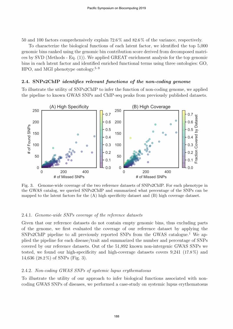
Fig. 3. Genome-wide coverage of the two reference datasets of SNPs2ChIP. For each phenotype inthe GWAS catalog, we queried SNPs2ChIP and summarized what percentage of the SNPs can bemapped to the latent factors for the (A) high specificity dataset and (B) high coverage dataset.

2.4.1. Genome-wide SNPs coverage of the reference datasets

Given that our reference datasets do not contain empty genomic bins, thus excluding partsof the genome, we first evaluated the coverage of our reference dataset by applying theSNPs2ChIP pipeline to all previously reported SNPs from the GWAS catalogue.1 We ap-plied the pipeline for each disease/trait and summarized the number and percentage of SNPscovered by our reference datasets. Out of the 51,892 known non-intergenic GWAS SNPs wetested, we found our high-specificity and high-coverage datasets covers 9,241 (17.8 %) and14,636 (28.2 %) of SNPs (Fig. 3).

2.4.2. Non-coding GWAS SNPs of systemic lupus erythematosus

To illustrate the utility of our approach to infer biological functions associated with non-coding GWAS SNPs of diseases, we performed a case-study on systemic lupus erythematosus


188

0.0 0.5 1.0 1.5 2.0 2.5 3.0 3.5-log_10(Binomial FDR)

HP:0012140

HP:0001888

HP:0001878

HP:0002917

HP:0004921

HP:0000121

HP:0200114

HP:0002643

HP:0000360

HP:0001281

Abnormality of cells of the lymphoid lineage

Lymphopenia

Hemolytic anemia

Hypomagnesemia

Abnormality of magnesium homeostasis

Nephrocalcinosis

Metabolic alkalosis

Neonatal respiratory distress

Tinnitus

Tetany 2.5 3.0 3.5 4.0 4.5

Binom. Fold

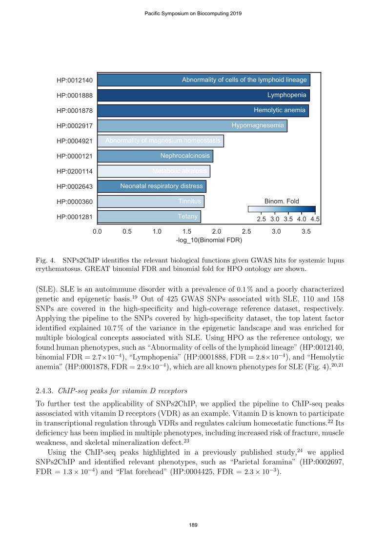
Fig. 4. SNPs2ChIP identifies the relevant biological functions given GWAS hits for systemic lupuserythematosus. GREAT binomial FDR and binomial fold for HPO ontology are shown.

(SLE). SLE is an autoimmune disorder with a prevalence of 0.1 % and a poorly characterizedgenetic and epigenetic basis.19 Out of 425 GWAS SNPs associated with SLE, 110 and 158SNPs are covered in the high-specificity and high-coverage reference dataset, respectively.Applying the pipeline to the SNPs covered by high-specificity dataset, the top latent factoridentified explained 10.7 % of the variance in the epigenetic landscape and was enriched formultiple biological concepts associated with SLE. Using HPO as the reference ontology, wefound human phenotypes, such as “Abnormality of cells of the lymphoid lineage” (HP:0012140,binomial FDR = 2.7×10−4), “Lymphopenia” (HP:0001888, FDR = 2.8×10−4), and “Hemolyticanemia” (HP:0001878, FDR = 2.9×10−4), which are all known phenotypes for SLE (Fig. 4).20,21

2.4.3. ChIP-seq peaks for vitamin D receptors

To further test the applicability of SNPs2ChIP, we applied the pipeline to ChIP-seq peaksassosciated with vitamin D receptors (VDR) as an example. Vitamin D is known to participatein transcriptional regulation through VDRs and regulates calcium homeostatic functions.22 Itsdeficiency has been implied in multiple phenotypes, including increased risk of fracture, muscleweakness, and skeletal mineralization defect.23

Using the ChIP-seq peaks highlighted in a previously published study,24 we appliedSNPs2ChIP and identified relevant phenotypes, such as “Parietal foramina” (HP:0002697,FDR = 1.3× 10−4) and “Flat forehead” (HP:0004425, FDR = 2.3× 10−3).


189

100 200 300 400 500Rank of Latent Factors Identified by Single SNP

0.25

0.50

0.75

1.00

Cum

ulat

ive

Freq

enci

es o

f Lat

ent F

acto

r Ide

ntifi

catio

n (A) All Latent Factors

Latent Factor Rank1st2nd4th3rd6th

1 2 3 4 5 6 7 8 9 10Rank of Latent Factors Identified by Single SNP

0.1

0.2

0.3

0.4

(B) Top 10 Latent FactorsLatent Factor Rank

1st2nd4th3rd6th

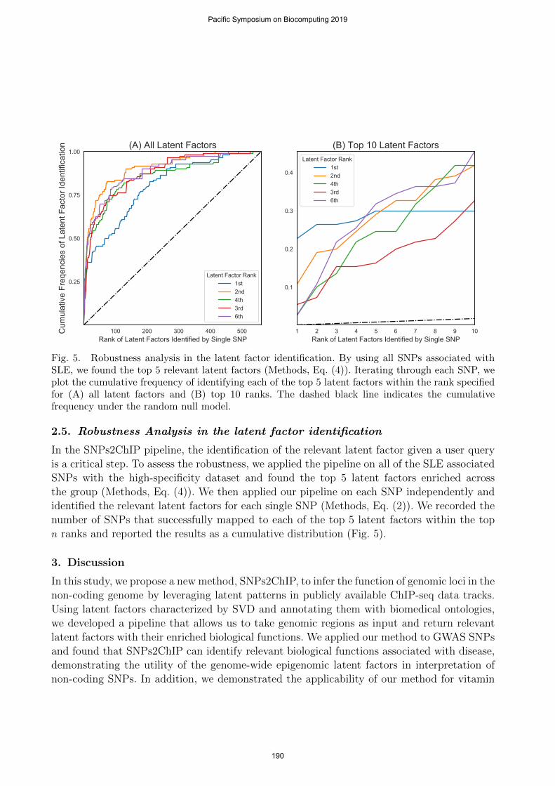
Fig. 5. Robustness analysis in the latent factor identification. By using all SNPs associated withSLE, we found the top 5 relevant latent factors (Methods, Eq. (4)). Iterating through each SNP, weplot the cumulative frequency of identifying each of the top 5 latent factors within the rank specifiedfor (A) all latent factors and (B) top 10 ranks. The dashed black line indicates the cumulativefrequency under the random null model.

2.5. Robustness Analysis in the latent factor identification

In the SNPs2ChIP pipeline, the identification of the relevant latent factor given a user queryis a critical step. To assess the robustness, we applied the pipeline on all of the SLE associatedSNPs with the high-specificity dataset and found the top 5 latent factors enriched acrossthe group (Methods, Eq. (4)). We then applied our pipeline on each SNP independently andidentified the relevant latent factors for each single SNP (Methods, Eq. (2)). We recorded thenumber of SNPs that successfully mapped to each of the top 5 latent factors within the topn ranks and reported the results as a cumulative distribution (Fig. 5).

3. Discussion

In this study, we propose a new method, SNPs2ChIP, to infer the function of genomic loci in thenon-coding genome by leveraging latent patterns in publicly available ChIP-seq data tracks.Using latent factors characterized by SVD and annotating them with biomedical ontologies,we developed a pipeline that allows us to take genomic regions as input and return relevantlatent factors with their enriched biological functions. We applied our method to GWAS SNPsand found that SNPs2ChIP can identify relevant biological functions associated with disease,demonstrating the utility of the genome-wide epigenomic latent factors in interpretation ofnon-coding SNPs. In addition, we demonstrated the applicability of our method for vitamin


190

D receptor ChIP-seq peaks, illustrating the utility of our approach for a diverse set of queries.Further, as shown in our robustness analysis, SNPs2ChIP has an ability to identify relevant

latent factors and functions even from a single SNP. This is a major advantage of SNPs2ChIP:it requires a minimal amount of input, one genomic coordinate, to infer biological function asit leverages latent patterns in the epigenome from across the whole genome.

As we rely on existing ChIP-seq data and we focused on lymphoblastoid cell lines, ourreference dataset has limited coverage of the genome, which is 12.1 % and 21.1 % for ourhigh-specificity and high-coverage datasets, respectively. While they still provide a GWAS setcoverage of 17.8 % and 28.2 %, a further expansion of the reference dataset may expand theapplicability of the methods.

The resources made available with this study, including the SNPs2ChIP pipeline as wellthe processed datasets, can provide a starting point to infer the biological functions of non-coding genomes. Combined with the expansion of large-scale epigenomic datasets,13,14 ourresults highlight the utility of latent factor analysis in interpreting the non-coding genome.

4. Methods

4.1. Featurization of the heterogeneous epigenetic assays

From the ChIP-Atlas database, we downloaded all available ChIP-seq peak files with FDRcorrected q-value threshold of 1.0× 10−5 for lymphoblastoid cell lines.13 Out of the 682 BEDfiles we obtained from the database, we found that 652 were non-empty and used these forour analysis. To featurize the data, we defined genomic bins of size 1kbp across all autosomesand saved them as a custom, genomic bin BED file. For the high-specificity dataset, we keptthe top 25,000 statistically significant peaks for each of the 652 BED files, to minimize theconfounders due to experimental design, and intersected each of them with the genomic binBED file using BEDTools.25 For the high-coverage dataset, we used all of the peaks in theBED files and intersected these with the genomic bin BED file. For each pair of genomic binand ChIP-seq assay from the BED intersection, we aggregated the negative log q-values intoa matrix and removed the genomic bins with no peaks. We generated two ChIP-maps, ourfeature matrices, for both the high-specificity and high-coverage datasets.

4.2. Batch normalization by surrogate variable analysis

We applied the SVA algorithm to the centered, scaled, and log-transformed input ChIP-map to eliminate technical effects which may obscure biological variation.18 SVA identifies,in an unsupervised manner, batches of variation across rows and columns of the input datamatrix that appear at a frequency greater than expected by chance; each of these batches isrepresented as a single surrogate variable. We observed that the metadata for the samples hada high rate of missingness; therefore, we devised a novel two-step approach for the removal oftechnical effects and the protection of biological effects of interest. In the first step, we foundstatistically significant associations between SVs and known covariates for the set of sampleswith non-missing metadata using linear regression, where highly significant p-values indicatestrong correlations between SV and covariates. As a result, we assigned labels to SVs based onthe likely biological or technical variation captured by each SV. In the second step, we removed


191

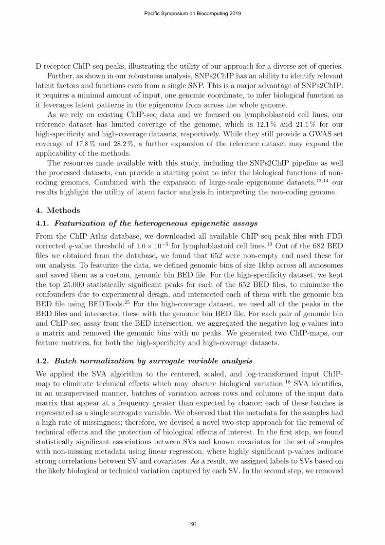
the SVs associated with biological effects of interest, and regressed out the remainder fromthe input data matrix. We investigated the quality of SVs and the preservation of biologicalsignal through manual inspection of principal component analysis plots.

4.3. Latent factor discovery with singular value decomposition (SVD)

We applied SVD for our SVA normalized matrix. The normalized matrix, which we denote asW , is of size N ×M , where N and M denote the number of ChIP-seq tracks and genomic bins,respectively. We obtained the matrix decomposition, W = UDV T , where U = (ui,k)i,k is anorthonormal matrix of size N ×K whose columns are left (ChIP-seq track) singular vectors,D is a diagonal matrix of size K ×K whose elements are singular values, and V = (vj,k)j,k isan orthonormal matrix of size M ×K whose columns are right (genomic bin) singular vectors.While singular values in D represent the magnitude of the latent factors, singular vectors inU and V summarize the strength of association between latent factors and ChIP-seq tracks,and latent factors and genomic bins, respectively.

4.3.1. Quantification of strength of associations between latent factor and genomic bins

To quantify the strength of associations between latent factor and genomic bins, we defineseveral quantitative scores built on the linear structures of latent factors.26,27 We first definethe factor score matrix for genomic bins as G = V D. Mathematically, the factor scorematrix is equivalent to the matrix consisting of principal component vectors.26 Each element ofthis matrix, which we call the genomic bin factor score and denote as gj,k, is the projectionof the j-th column vector in the input matrix W of length N , which represents the epigeneticlandscape of j-th genomic bin across samples, to the k-th latent factor (principal component).26

To quantify the relative importance of a genomic bin for a given latent factor, we definethe genomic bin contribution score for k-th latent factor by squaring the genomic binfactor scores for k-th factor and normalizing it across latent factors, i.e.

cntrbink (j) = (vj,k)2 (1)

The sum of genomic bin contribution scores across genomic bins is guaranteed to be one, i.e.∑j cntrbink (j) = 1, because V is an orthonormal matrix. One can interpret the score as the

percent-importance of a genomic bin for the factor.26,27

Similarly, to quantify the relative importance of a latent factor for a given genomic bin,we define the genomic bin squared cosine score for j-th genomic bin as follows:

cos2binj (k) =

(gj,k)2∑k′(gj,k′)2

(2)

The sum of genomic bin squared cosine scores across latent factors is guaranteed to be one,i.e.

∑k cos2j

bin(k) = 1, because of the demoninator in Eq. (2). One can interpret the score as

the relative importance of latent factors for a particular genomic bin.

4.3.2. Quantification of strength of associations between latent factor and samples

We also define the same set of scores to quantify the strength of associations between latentfactors and samples. We first define the factor score matrix for samples as S = UD =


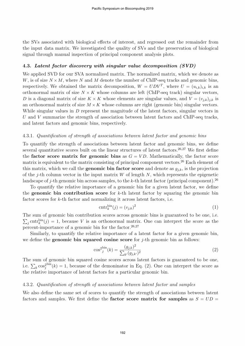
192

(si,k)i,k. To quantify the relative importance of samples to latent factors and latent factors tosamples, we define the sample contribution score and the sample squared cosine scoresas follows:

cntrsamplek (i) = (ui,k)2 ; cos2

samplei (k) =

(si,k)2∑k′(si,k′)2

(3)

With these scoring systems we can effectively quantify the associations among latent factors,genomic bins, and samples.

4.4. GREAT analysis for biological characterization of latent factor

To characterize the functions of latent factors, we applied GREAT version 3.0.0 to each latentfactor.9 Using ontology-based gene annotations as a reference, GREAT takes a set of genomicregions as an input and reports enriched ontology terms. In our analysis, we focused ongene ontology (GO), human phenotype ontology (HPO), and Mouse Genome Informatics(MGI) phenotype ontology.5–8 For each latent factor, we created the query files for GREATby selecting the top 5,000 genomic bins ranked by genomic bin contribution score (Eq. (1))and applied GREAT for these queries using default parameters.9,27 Given our interest tocharacterize the putative functions of non-coding genomes, we focused on the GREAT binomialtest and collected summary statistics, such as binomial p-value, binomial FDR, and binomialfold change. We sorted the functional terms outputted by GREAT using binomial FDR andidentified the ontology terms that most characterize the function of each latent factor.

4.5. Application of the SNPs2ChIP pipeline for GWAS hits and ChIP-seqpeaks

The SNPs2ChIP pipeline consists of three steps: (1) identification of the genomic bins givena user query, (2) identification of the relevant latent factors for the genomic bins, and (3)reporting the results of GREAT enrichment for the relevant latent factors.

4.5.1. Identification of the genomic bin for a given user’s query

SNPs2ChIP takes genomic coordinates as an input. For GWAS SNPs and ChIP-seq peaks,one first needs to obtain their genomic coordinates. These coordinates are then mapped tothe corresponding genomic bins, if they contain a ChIP-seq peak.

4.5.2. Identification of the relevant latent factor for the genomic bins

We identify the relevant latent factors for a given genomic bin by genomic bin squared co-sine score (Eq. (2)). We can identify the relevant latent factors for multiple genomic bins,which typically corresponds to multiple inputs, by taking a weighted average of genomic binsquared cosine scores. Let’s denote J = {j1, . . . , jm} be the set of genomic bins of interest and{w1, . . . , wm} be the corresponding weights. We defined the weighted average of genomic binsquared cosine score as follows:

cos2binJ (k) =

∑j∈J wj · cos2binj (k)∑

j∈J wj(4)


193

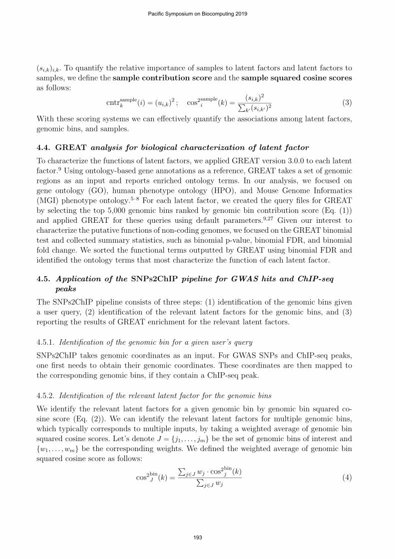
We set the default value of weights to be uniform, i.e. {w1, . . . , wm} = {1/m, . . . , 1/m} but theuser can specify a set of weights based on external knowledge, such as statistical significanceand effect size estimates from GWAS. Once we identify the relevant latent factors, we reportthe results of GREAT enrichment analysis to the users.

4.5.3. Systematic application of SNPs2ChIP for known GWAS hits

We downloaded the GWAS Catalog v1.0 from the European Bioinformatics Institute, contain-ing 82,735 curated SNPs.1 The catalog was subsequently filtered to exclude SNPs that wereclassified as intergenic to focus on SNPs associated with transcriptional cis-regulation, result-ing 51,892 SNPs. Individual SNPs were processed by the SNPs2ChIP pipeline to determinetheir enriched phenotype. To validate the robustness of the method, SNPs were grouped bydisease and run to determine their combined, enriched phenotype. As the pipeline is designedfor high-throughput data analysis, querying thousands of SNPs was done in mere seconds.

Acknowledgments

This study was originally conceived as a class project for BIOMEDIN212: “Introduction toBiomedical Informatics Research Methodology” at Stanford University. We thank the teach-ing team: Hunter Boyce, Steven Bagley, and Russ B. Altman, as well as our classmates forconstructive comments. C.S. is supported by the Stanford University BD2K Training Grant(T32 LM012409). L.K. is supported by the Stanford University Biomedical Informatics Train-ing Grant (T15 LM007033). Y.T. is supported by the Funai Overseas Scholarship from FunaiFoundation for Information Technology and the Stanford University School of Medicine.

Author contributions

Y.T. conceived and designed the study. S.A., L.K., C.S., and Y.T. designed and carried outthe computational analyses. The manuscript was written by S.A., L.K., C.S., and Y.T.

Availability

All the source code used in this project as well as pre-processed reference dataset are availablein our GitHub repository: https://github.com/lkalesinskas/SNPs2ChIP.

References

1. J. MacArthur, E. Bowler, M. Cerezo et al., The new NHGRI-EBI Catalog of published genome-wide association studies (GWAS Catalog), Nucleic Acids Research 45, D896 (2017).

2. P. M. Visscher, N. R. Wray, Q. Zhang et al., 10 Years of GWAS Discovery: Biology, Function,and Translation., American journal of human genetics 101, 5 (2017).

3. F. Zhang and J. R. Lupski, Non-coding genetic variants in human disease, Human MolecularGenetics 24, R102 (2015).

4. T. S. Furey, ChIP–seq and beyond: New and improved methodologies to detect and characterizeprotein–DNA interactions, Nature Reviews Genetics 13, 840 (2012).

5. M. Ashburner, C. A. Ball, J. A. Blake et al., Gene ontology: Tool for the unification of biology.The Gene Ontology Consortium, Nature Genetics 25, 25 (2000).


194

https://github.com/lkalesinskas/SNPs2ChIP

6. The Gene Ontology Consortium, Expansion of the Gene Ontology knowledgebase and resources,Nucleic Acids Research 45, D331 (2017).

7. S. Kohler, N. A. Vasilevsky, M. Engelstad et al., The Human Phenotype Ontology in 2017,Nucleic Acids Research 45, D865 (2017).

8. J. A. Blake, J. T. Eppig, J. A. Kadin et al., Mouse Genome Database (MGD)-2017: Communityknowledge resource for the laboratory mouse, Nucleic Acids Research 45, D723 (2017).

9. C. Y. McLean, D. Bristor, M. Hiller et al., GREAT improves functional interpretation of cis-regulatory regions., Nature biotechnology 28, 495 (2010).

10. ENCODE Project Consortium, An integrated encyclopedia of DNA elements in the humangenome., Nature 489, 57 (2012).

11. Roadmap Epigenomics Consortium, A. Kundaje, W. Meuleman et al., Integrative analysis of111 reference human epigenomes, Nature 518, 317 (2015).

12. G. Consortium, Genetic effects on gene expression across human tissues, Nature 550, 204 (2017).13. S. Oki, T. Ohta, G. Shioi et al., Integrative analysis of transcription factor occupancy at en-

hancers and disease risk loci in noncoding genomic regions, bioRxiv (2018).14. J. Cheneby, M. Gheorghe, M. Artufel, A. Mathelier and B. Ballester, ReMap 2018: An updated

atlas of regulatory regions from an integrative analysis of DNA-binding ChIP-seq experiments,Nucleic Acids Research 46, D267 (2018).

15. S. A. Lambert, A. Jolma, L. F. Campitelli et al., The Human Transcription Factors, Cell 172,650 (2018).

16. J. Ernst and M. Kellis, Discovery and characterization of chromatin states for systematic anno-tation of the human genome, Nature Biotechnology 28, 817 (2010).

17. M. M. Hoffman, O. J. Buske, J. Wang et al., Unsupervised pattern discovery in human chromatinstructure through genomic segmentation, Nature Methods 9, 473 (2012).

18. J. T. Leek, W. E. Johnson, H. S. Parker, A. E. Jaffe and J. D. Storey, The SVA package for remov-ing batch effects and other unwanted variation in high-throughput experiments, Bioinformatics28, 882 (2012).

19. G. C. Tsokos, Systemic Lupus Erythematosus, New England Journal of Medicine 365, 2110(2011).

20. S. J. Rivero, E. Dıaz-Jouanen and D. Alarcon-Segovia, Lymphopenia In Systemic Lupus Ery-thematosus, Arthritis & Rheumatism 21, 295 (1978).

21. S. I. G. Kokori, J. P. A. Ioannidis, M. Voulgarelis, A. G. Tzioufas and H. M. Moutsopoulos,Autoimmune hemolytic anemia in patients with systemic lupus erythematosus, The AmericanJournal of Medicine 108, 198 (2000).

22. L. L. Issa, G. M. Leong and J. A. Eisman, Molecular mechanism of vitamin D receptor action,Inflammation Research 47, 451 (1998).

23. M. F. Holick and T. C. Chen, Vitamin D deficiency: A worldwide problem with health conse-quences, The American Journal of Clinical Nutrition 87, 1080S (2008).

24. S. V. Ramagopalan, A. Heger, A. J. Berlanga et al., A ChIP-seq defined genome-wide map ofvitamin D receptor binding: Associations with disease and evolution., Genome research 20, 1352(2010).

25. A. R. Quinlan and I. M. Hall, BEDTools: A flexible suite of utilities for comparing genomicfeatures, Bioinformatics 26, 841 (2010).

26. H. Abdi and L. J. Williams, Principal component analysis, Wiley Interdisciplinary Reviews:Computational Statistics 2, 433 (2010).

27. Y. Tanigawa, J. Li, J. M. Justesen et al., Components of genetic associations across 2,138 phe-notypes in the UK Biobank highlight novel adipocyte biology, bioRxiv (2018).


195

Documents

SNPs2ChIP: Latent Factors of ChIP-seq to infer functions ...psb.stanford.edu/psb-online/proceedings/psb19/anand.pdf · To normalize batch e ects in each ChIP-map, we applied the SVA