SOBOLEV METRICS ON DIFFEOMORPHISM GROUPS AND THE DERIVED ...michor/landmarks.pdf · sobolev metrics on diffeomorphism groups and the derived geometry of spaces of submanifolds mario

SOBOLEV METRICS ON DIFFEOMORPHISM GROUPS AND

THE DERIVED GEOMETRY OF SPACES OF SUBMANIFOLDS

MARIO MICHELI, PETER W. MICHOR AND DAVID MUMFORD

Dedicated to I.R. Shafarevich on the occasion of his 90th birthday

Abstract. Given a finite dimensional manifold N , the group DiffS(N) of

diffeomorphism of N which fall suitably rapidly to the identity, acts on the

manifold B(M,N) of submanifolds on N of diffeomorphism type M where Mis a compact manifold with dimM < dimN . For a right invariant weak

Riemannian metric on DiffS(N) induced by a quite general operator L :

XS(N)→ Γ(T ∗N⊗vol(N)), we consider the induced weak Riemannian metricon B(M,N) and we compute its geodesics and sectional curvature. For that

we derive a covariant formula for curvature in finite and infinite dimensions,

we show how it makes O’Neill’s formula very transparent, and we use it finallyto compute sectional curvature on B(M,N).

1. Introduction

It was 46 years ago that Arnold discovered an amazing link between Euler’sequation for incompressible non-viscous fluid flow and geodesics in the group ofvolume preserving diffeomorphisms SDiff(Rn) under the L2-metric [2]. One goalin this paper is to extend his ideas to a large class of Riemannian metrics on thegroup of all diffeomorphisms DiffS(N) falling suitably to the identity, of any finitedimensional manifold N . The resulting geodesic equations are integro-differentialequations for fluid-like flows onN determined by an initial velocity field. In previouspapers [13, 11, 9], we have looked at the special case where N = Rn and the metricis a sum of Sobolev norms on each component of the tangent vector but here wedevelop the formalism to work in a very general setting.

The extra regularity given by using higher order norms means that these metricson the group of diffeomorphisms can induce a metric on many quotient spaces ofthe diffeomorphism group modulo a subgroup. This paper focuses on the spaceof submanifolds of N diffeomorphic to some M which we denote by B(M,N).DiffS(N) acts on B(M,N) with open orbits, one for each isotopy type of embeddingof M in N . The spaces B may be called the Chow manifolds of N by analogy withthe Chow varieties of algebraic geometry, or non-linear Grassmannians becauseof their analogy with the Grassmannian of linear subspaces of a projective space.

Date: March 1, 2015.

2000 Mathematics Subject Classification. Primary 58B20, 58D15, 37K65.MM was supported by ONR grant N00014-09-1-0256, PWM was supported by FWF-project

21030, DM was supported by NSF grant DMS-0704213, and all authors where supported by NSFgrant DMS-0456253.

1

2 MARIO MICHELI, PETER W. MICHOR AND DAVID MUMFORD

The key point is that the metrics we study will descend to the spaces B(M,N) sothat the map DiffS(N) → B(M,N) (given by the group action on a base point)is a Riemannian submersion. Geodesics from one submanifold to another may bethought of as deformations of one into the other realized by a flow on N of minimalenergy.

In the special case where M is a finite set of points, B(M,N) is called thespace of landmark point sets in N . This has been used extensively by statisticiansfor example and is the subject of our previous paper [9]. The case B(S1,R2) isthe space of all simple closed plane curves and has been studied in many metrics,see [8, 12, 15] for example. This and the case B(S2,R3) of spheres in 3-space havehad many applications to medical imaging, constructing optimal warps of variousbody parts or sections of body parts from one medical scan to another [14, 19].

The high point of Arnold’s analysis was his determination of the sectional curva-tures in the group of volume preserving diffeomorphisms. This has had considerableimpact on the analysis of the stability and instability of incompressible fluid flow.A similar formula for sectional curvature of B(M,N) may be expected to shed lighton how stable or unstable geodesics are in this space, e.g. whether they are uniqueand effective for medical applications.

Computing this curvature required a new formula. In general, the induced innerproduct on the cotangent space of a submersive quotient is much more amenable tocalculations than the inner product on the tangent space. The first author founda new formula for the curvature tensor of a Riemannian manifold which uses onlyderivatives of the former, the dual metric tensor. This result, Mario’s formula, isproven in section 2. In this section we also define a new class of infinite dimensionalRiemannian manifolds, robust Riemannian manifolds to which Mario’s formula andour analysis of submersive quotients applies. We also obtain a transparent newproof of O’Neill’s curvature fomula. This class of manifolds builds on the theoryof convenient infinite dimensional manifolds, see [7]. To facilitate readability thistheory is summarized in an Appendix.

In section 3, we describe diffeomorphism groups of a finite dimensional manifoldN consisting of diffeomorphisms which decrease suitably rapidly to the identity onN if we move to infinity on N ; only these admit charts and are a regular Lie groups.We shall denote by DiffS(N) any of these groups in order to simplify notation, andby XS(N) the corresponding Lie algebra of suitably decreasing vector fields on N .We introduce a very general class of Riemannian metrics given by a positive definiteself-adjoint differential operator L from the space of smooth vector fields on N tothe space of measure-valued 1-forms. This defines an inner product on vector fieldsX,Y by:

〈X,Y 〉L =

∫N

(LX, Y ).

Note that LX paired with Y gives a measure on N hence can be integrated withoutassuming N carries any further structure. Under suitable assumptions, the inverseof L is given by a kernel K(x, y) on N × N with values in p∗1TN ⊗ p∗2TN . Wethen describe the geodesic equation in DiffS(N) for these metrics. It is especiallysimple written in terms of the momentum. If ϕ(t) ∈ DiffS(N) is the geodesic, then

SOBOLEV CURVATURE 3

X(t) = ∂t(ϕ)ϕ−1 is a time varying vector field on N and its momentum is simplyLX(t).

In section 4 we introduce the induced metrics on B(M,N). We give the geodesicequation for these metrics also using momentum. One of the keys to working inthis space is to define a convenient set of vector fields and forms on B in terms ofauxiliary forms and vector fields on N . In this way, differential geometry on B canbe reduced to calculations on N . Lie derivatives on N are especially useful here.

In the final section 5, we compute the sectional curvatures of B(M,N). LikeArnold’s formula, we get a formula with several terms each of which seems to playa different role. The first involves the second derivatives of K and the others areexpressed in terms which we call force and stress. Force is the bilinear versionof the acceleration term in the geodesic equation and stress is a derivative of onevector field with respect to the other, half of a Lie bracket, defined in what areessentially local coordinates. For the landmark space case, we proved this formulain our previous paper [9]. We hope that the terms in this formula will be elucidatedby further study and analysis of specific cases.

2. A Covariant Formula for Curvature

2.1. Covariant derivative. Let (M, g) be a (finite dimensional) Riemannianmanifold. There will be some formulae which are valid for infinite dimensionalmanifolds and we will introduce definitions for these below. For each x ∈ M weview the metric also as a bijective mapping gx : TxM → T ∗xM . Then g−1 is themetric on the cotangent bundle as well as the morphism T ∗M → TM . For a 1-formα ∈ Ω1(M) = Γ(T ∗M) we consider the ‘sharp’ vector field α] = g−1α ∈ X(M). Ifα = αidx

i, then α] = αigij∂j is just the vector field obtained from α by ‘raising

indices’. Similarly, for a vector field X ∈ X(M) we consider the ‘flat’ 1-formX[ = gX. If X = Xi∂i, then X[ = Xigijdx

j is the 1-form obtained from X by‘lowering indices’. Note that

(1) α(β]) = g−1(α, β) = g(α], β]) = β(α]).

Our aim is to express the sectional curvature of g in terms of α, β alone. It isimportant that the exterior derivative satisfies:

(2) dα(β], γ]) = (β])α(γ])− (γ])α(β])− α([β], γ]])

We recall the definition of the Levi-Civita covariant derivative ∇ and its basicproperties:

2g(∇XY,Z) = X(g(Y,Z)) + Y (g(Z,X))− Z(g(X,Y ))(3)

− g(X, [Y,Z]) + g(Y, [Z,X]) + g(Z, [X,Y ])

(∇Xα)(Y ) = Xα(Y )− α(∇XY )(4)

g((∇Xα)], Y ) = (∇Xα)(Y ) = X(α(Y ))− α(∇XY )

= Xg(α], Y )− g(α],∇XY ) = g(∇Xα], Y ) =⇒

∇X(α]) = (∇Xα)](5)

Xg−1(α, β) = g−1(∇Xα, β) + g−1(α,∇Xβ)


∇α]β −∇β]α = g[α], β]] = [α], β]][

From this follows

2(∇α]β)(γ]) = 2g−1(∇α]β, γ) = 2g((∇α]β)], γ]) = 2g(∇α]β], γ]) =

= α]g−1(β, γ) + β]g−1(γ, α)− γ]g−1(α, β))

− g−1(α, [β], γ]][) + g−1(β, [γ], α]][) + g−1(γ, [α], β]][)

= α]β(γ]) + β]γ(α])− γ]β(α])

− α([β], γ]]) + β([γ], α]]) + γ([α], β]])

= β]γ(α])− α([β], γ]]) + γ([α], β]])− dβ(γ], α])

= α]γ(β])− β]α(γ]) + γ]α(β]) + dα(β], γ])− dβ(γ], α])− dγ(α], β])(7)

2.2. Theorem. (Mario’s Formula) Assume that all 1-forms α, β, γ, δ ∈ Ω1g(M)

are closed. Then curvature is given by:

g(R(α], β])γ], δ]

)= R1 +R2 +R3

R1 = 14

(−α]γ]δ(β]) + α]δ]β(γ]) + β]γ]δ(α])− β]δ]α(γ])

−γ]α]δ(β]) + γ]β]δ(α]) + δ]α]β(γ])− δ]β]α(γ]))

R2 = 14

(−g−1

(d(γ(β])), d(δ(α]))

)+ g−1

(d(γ(α])), d(δ(β]))

))R3 = 1

4

(g([δ], α]], [β], γ]]

)− g([δ], β]], [α], γ]]

)+ 2g

([α], β]], [γ], δ]]

))For the numerator of sectional curvature we get

g(R(α], β])β], α]

)= R1 +R2 +R3

R1 = 12

(α]α](‖β‖2)− (α]β] + β]α])g−1(α, β) + β]β](‖α‖2)

)= 1

2

(α]β([α], β]])− β]α([α], β]])

)R2 = 1

4

(‖d(g−1(α, β))‖2 − g−1

(d(‖α‖2), d(‖β‖2)

)R3 = − 3

4

∥∥[α], β]]∥∥2

g

Recall that sectional curvature is then

k(α], β]) =g(R(α], β])β], α]

)‖α‖2‖β‖2 − g−1(α, β)2

Proof. We shall need that for a function f we have:

(∇β]γ)]f = df((∇β]γ)]) = g−1(df,∇β]γ) = β]g−1(df, γ)− g−1(∇β]df, γ)

= β]γ]f −∇β]df(γ]) = β]γ]f − 12β

]df(γ]) + 12df

]γ(β])− 12γ

]β(df ])

= 12df

]γ(β]) + 12 [β], γ]]f = 1

2d(γ(β]))(df ]) + 12 [β], γ]]f(8)

For the three summands in the curvature formula, by multiple uses of formulas (2)and (7) and the closedness of α, β, γ, δ, a straightforward calculation gives us:

4(∇α]∇β]γ)(δ]) =

= 2α](∇β]γ)(δ])− 2(∇β]γ)]δ(α]) + 2δ]α((∇β]γ)])− 2d(∇β]γ)(δ], α])

= 2α](∇β]γ)(δ])− d(γ(β]))(d(δ(α])])− [β], γ]]δ(α])

SOBOLEV CURVATURE 5

+ 2α](∇β]γ)(δ]) + 2(∇β]γ)([δ], α]]) = · · · =

= −g−1(d(γ(β])), d(δ(α]))

)+ g([δ], α]], [β], γ]]

)+ 2α]β]γ(δ])− 2α]γ]δ(β]) + α]δ]β(γ])− [β], γ]]δ(α]) + δ]α]β(γ])

and similarly

− 4(∇β]∇α]γ)(δ]) = +g−1(d(γ(α])), d(δ(β]))

)− g([δ], β]], [α], γ]]

)− 2β]α]γ(δ]) + 2β]γ]δ(α])− β]δ]α(γ]) + [α], γ]]δ(β])− δ]β]α(γ])

− 2(∇[α],β]]γ)(δ]) =

= −[α], β]]γ(δ]) + γ]δ([α], β]])− δ]γ([α], β]])− d[α], β]][(γ], δ])

= −[α], β]]γ(δ]) + g([α], β]], [γ], δ]]

)Now we can compute the curvature (remember that dα = dβ = · · · = 0):

4g(R(α], β])γ], δ]

)= 4δ

(R(α], β])γ]

)= 4δ

(∇α]∇β]γ] −∇β]∇α]γ] −∇[α],β]]γ

])

= 4(∇α]∇β]γ −∇β]∇α]γ −∇[α],β]]γ

)(δ])

= −g−1(d(γ(β])), d(δ(α]))

)+ g−1

(d(γ(α])), d(δ(β]))

)+ g([δ], α]], [β], γ]]

)− g([δ], β]], [α], γ]]

)+ 2g

([α], β]], [γ], δ]]

)− α]γ]δ(β]) + α]δ]β(γ]) + β]γ]δ(α])− β]δ]α(γ])

− γ]α]δ(β]) + γ]β]δ(α]) + δ]α]β(γ])− δ]β]α(γ])

For the sectional curvature expression this simplifies (as always, for closed 1-forms)to the expression in the theorem. The two versions of R1 correspond to each other,using dα = 0 and dβ = 0.

2.3. Mario’s formula in coordinates. The formula for sectional curvaturebecomes especially transparent if we expand it in coordinates. Assume that α =αidx

i, β = βidxi where the coefficients αi, βi are constants, hence α, β are closed.

Then α] = gijαi∂j , β] = gijβi∂j . Substituting these in the terms of the right hand

side of Mario’s formula for sectional curvature, we get:

2nd deriv. terms = 2R1 = 2α]α](‖β‖2) + 2β]β](‖α‖2)− 2(α]β] + β]α])g−1(α, β)

= 2αigis(αjg

jt(βkβlgkl),t),s + 2βig

is(βjgjt(αkαlg

kl),t),s

− 2αigis(βjg

jt(βkαlgkl),t),s − 2βig

is(αjgjt(αkβlg

kl),t),s

= 2(αiβk − αkβi) · (αjβl − αlβj) · gis(gjtgkl,t ),s

1st deriv. terms = 4R2 = ‖d(g−1(α, β))‖2 − g−1(d(‖α‖2), d(‖β‖2)

)= (αiβjg

ij),sgst(αlβkg

kl),t − (αiαjgij),sg

st(βkβlgkl),t

= − 12 (αiβk − αkβi) · (αjβl − αlβj) · gij,sgstgkl,t

Lie bracket = [α], β]] =(αig

is(βkgkt),s − βigis(αkgkt),s

)∂t

= (αiβk − αkβi)gisgkt,s ∂tLie bracket term = 4R3 = −3g

([α], β]], [α], β]]

)= −3(αiβk − αkβi) · (αjβl − αlβj) · gisgkp,s gpqgjtg

lq,t


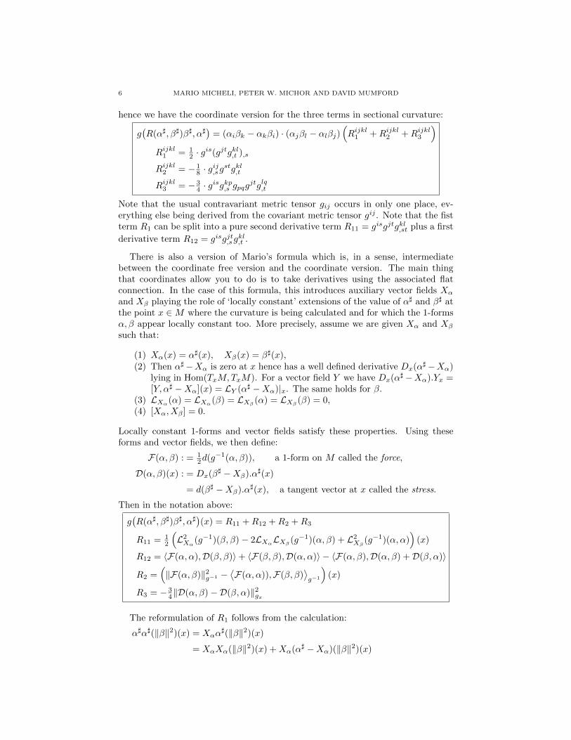
hence we have the coordinate version for the three terms in sectional curvature:

g(R(α], β])β], α]

)= (αiβk − αkβi) · (αjβl − αlβj)

(Rijkl1 +Rijkl2 +Rijkl3

)Rijkl1 = 1

2 · gis(gjtgkl,t ),s

Rijkl2 = − 18 · g

ij,sg

stgkl,t

Rijkl3 = − 34 · g

isgkp,s gpqgjtglq,t

Note that the usual contravariant metric tensor gij occurs in only one place, ev-erything else being derived from the covariant metric tensor gij . Note that the fistterm R1 can be split into a pure second derivative term R11 = gisgjtgkl,st plus a first

derivative term R12 = gisgjt,s gkl,t .

There is also a version of Mario’s formula which is, in a sense, intermediatebetween the coordinate free version and the coordinate version. The main thingthat coordinates allow you to do is to take derivatives using the associated flatconnection. In the case of this formula, this introduces auxiliary vector fields Xα

and Xβ playing the role of ‘locally constant’ extensions of the value of α] and β] atthe point x ∈M where the curvature is being calculated and for which the 1-formsα, β appear locally constant too. More precisely, assume we are given Xα and Xβ

such that:

(1) Xα(x) = α](x), Xβ(x) = β](x),(2) Then α]−Xα is zero at x hence has a well defined derivative Dx(α]−Xα)

lying in Hom(TxM,TxM). For a vector field Y we have Dx(α]−Xα).Yx =[Y, α] −Xα](x) = LY (α] −Xα)|x. The same holds for β.

(3) LXα(α) = LXα(β) = LXβ (α) = LXβ (β) = 0,(4) [Xα, Xβ ] = 0.

Locally constant 1-forms and vector fields satisfy these properties. Using theseforms and vector fields, we then define:

F(α, β) : = 12d(g−1(α, β)), a 1-form on M called the force,

D(α, β)(x) : = Dx(β] −Xβ).α](x)

= d(β] −Xβ).α](x), a tangent vector at x called the stress.

Then in the notation above:

g(R(α], β])β], α]

)(x) = R11 +R12 +R2 +R3

R11 = 12

(L2Xα(g−1)(β, β)− 2LXαLXβ (g−1)(α, β) + L2

Xβ(g−1)(α, α)

)(x)

R12 = 〈F(α, α),D(β, β)〉+ 〈F(β, β),D(α, α)〉 − 〈F(α, β),D(α, β) +D(β, α)〉

R2 =(‖F(α, β)‖2g−1 −

⟨F(α, α)),F(β, β)

⟩g−1

)(x)

R3 = − 34‖D(α, β)−D(β, α)‖2gx

The reformulation of R1 follows from the calculation:

α]α](‖β‖2)(x) = Xαα](‖β‖2)(x)

= XαXα(‖β‖2)(x) +Xα(α] −Xα)(‖β‖2)(x)

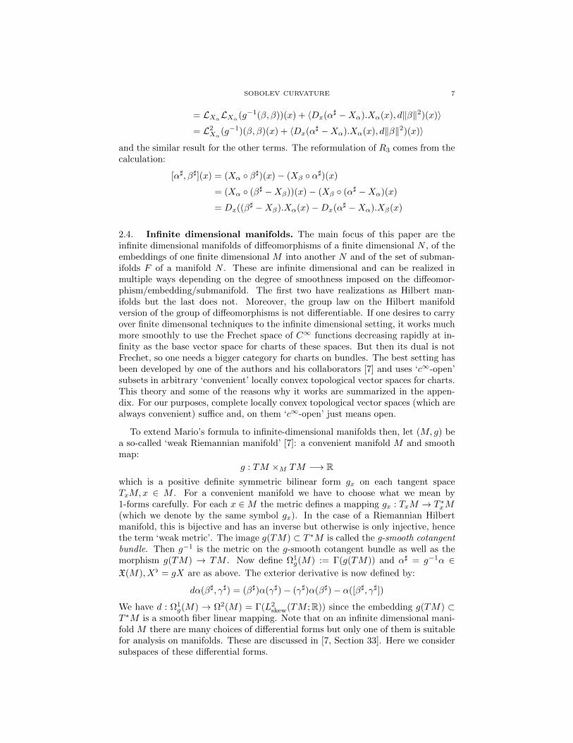
SOBOLEV CURVATURE 7

= LXαLXα(g−1(β, β))(x) + 〈Dx(α] −Xα).Xα(x), d‖β‖2)(x)〉

= L2Xα(g−1)(β, β)(x) + 〈Dx(α] −Xα).Xα(x), d‖β‖2)(x)〉

and the similar result for the other terms. The reformulation of R3 comes from thecalculation:

[α], β]](x) = (Xα β])(x)− (Xβ α])(x)

= (Xα (β] −Xβ))(x)− (Xβ (α] −Xα)(x)

= Dx((β] −Xβ).Xα(x)−Dx(α] −Xα).Xβ(x)

2.4. Infinite dimensional manifolds. The main focus of this paper are theinfinite dimensional manifolds of diffeomorphisms of a finite dimensional N , of theembeddings of one finite dimensional M into another N and of the set of subman-ifolds F of a manifold N . These are infinite dimensional and can be realized inmultiple ways depending on the degree of smoothness imposed on the diffeomor-phism/embedding/submanifold. The first two have realizations as Hilbert man-ifolds but the last does not. Moreover, the group law on the Hilbert manifoldversion of the group of diffeomorphisms is not differentiable. If one desires to carryover finite dimensonal techniques to the infinite dimensional setting, it works muchmore smoothly to use the Frechet space of C∞ functions decreasing rapidly at in-finity as the base vector space for charts of these spaces. But then its dual is notFrechet, so one needs a bigger category for charts on bundles. The best setting hasbeen developed by one of the authors and his collaborators [7] and uses ‘c∞-open’subsets in arbitrary ‘convenient’ locally convex topological vector spaces for charts.This theory and some of the reasons why it works are summarized in the appen-dix. For our purposes, complete locally convex topological vector spaces (which arealways convenient) suffice and, on them ‘c∞-open’ just means open.

To extend Mario’s formula to infinite-dimensional manifolds then, let (M, g) bea so-called ‘weak Riemannian manifold’ [7]: a convenient manifold M and smoothmap:

g : TM ×M TM −→ Rwhich is a positive definite symmetric bilinear form gx on each tangent spaceTxM,x ∈ M . For a convenient manifold we have to choose what we mean by1-forms carefully. For each x ∈M the metric defines a mapping gx : TxM → T ∗xM(which we denote by the same symbol gx). In the case of a Riemannian Hilbertmanifold, this is bijective and has an inverse but otherwise is only injective, hencethe term ‘weak metric’. The image g(TM) ⊂ T ∗M is called the g-smooth cotangentbundle. Then g−1 is the metric on the g-smooth cotangent bundle as well as themorphism g(TM) → TM . Now define Ω1

g(M) := Γ(g(TM)) and α] = g−1α ∈X(M), X[ = gX are as above. The exterior derivative is now defined by:

dα(β], γ]) = (β])α(γ])− (γ])α(β])− α([β], γ]])

We have d : Ω1g(M) → Ω2(M) = Γ(L2

skew(TM ;R)) since the embedding g(TM) ⊂T ∗M is a smooth fiber linear mapping. Note that on an infinite dimensional mani-fold M there are many choices of differential forms but only one of them is suitablefor analysis on manifolds. These are discussed in [7, Section 33]. Here we considersubspaces of these differential forms.


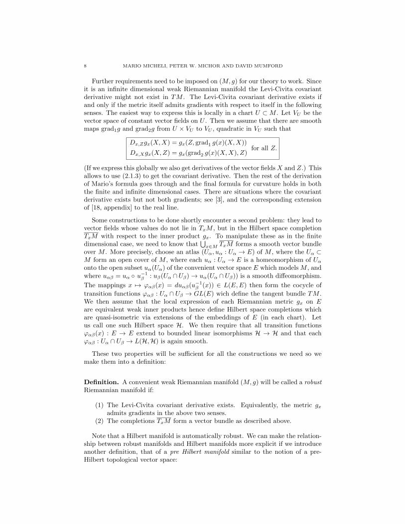
Further requirements need to be imposed on (M, g) for our theory to work. Sinceit is an infinite dimensional weak Riemannian manifold the Levi-Civita covariantderivative might not exist in TM . The Levi-Civita covariant derivative exists ifand only if the metric itself admits gradients with respect to itself in the followingsenses. The easiest way to express this is locally in a chart U ⊂M . Let VU be thevector space of constant vector fields on U . Then we assume that there are smoothmaps grad1g and grad2g from U × VU to VU , quadratic in VU such that

Dx,Zgx(X,X) = gx(Z, grad1 g(x)(X,X))

Dx,Xgx(X,Z) = gx(grad2 g(x)(X,X), Z)for all Z.

(If we express this globally we also get derivatives of the vector fieldsX and Z.) Thisallows to use (2.1.3) to get the covariant derivative. Then the rest of the derivationof Mario’s formula goes through and the final formula for curvature holds in boththe finite and infinite dimensional cases. There are situations where the covariantderivative exists but not both gradients; see [3], and the corresponding extensionof [18, appendix] to the real line.

Some constructions to be done shortly encounter a second problem: they lead tovector fields whose values do not lie in TxM , but in the Hilbert space completionTxM with respect to the inner product gx. To manipulate these as in the finitedimensional case, we need to know that

⋃x∈M TxM forms a smooth vector bundle

over M . More precisely, choose an atlas (Uα, uα : Uα → E) of M , where the Uα ⊂M form an open cover of M , where each uα : Uα → E is a homeomorphism of Uαonto the open subset uα(Uα) of the convenient vector space E which models M , andwhere uαβ = uα u−1

β : uβ(Uα ∩Uβ)→ uα(Uα ∩Uβ)) is a smooth diffeomorphism.

The mappings x 7→ ϕαβ(x) = duαβ(u−1β (x)) ∈ L(E,E) then form the cocycle of

transition functions ϕαβ : Uα ∩ Uβ → GL(E) wich define the tangent bundle TM .We then assume that the local expression of each Riemannian metric gx on Eare equivalent weak inner products hence define Hilbert space completions whichare quasi-isometric via extensions of the embeddings of E (in each chart). Letus call one such Hilbert space H. We then require that all transition functionsϕαβ(x) : E → E extend to bounded linear isomorphisms H → H and that eachϕαβ : Uα ∩ Uβ → L(H,H) is again smooth.

These two properties will be sufficient for all the constructions we need so wemake them into a definition:

Definition. A convenient weak Riemannian manifold (M, g) will be called a robustRiemannian manifold if:

(1) The Levi-Civita covariant derivative exists. Equivalently, the metric gxadmits gradients in the above two senses.

(2) The completions TxM form a vector bundle as described above.

Note that a Hilbert manifold is automatically robust. We can make the relation-ship between robust manifolds and Hilbert manifolds more explicit if we introduceanother definition, that of a pre Hilbert manifold similar to the notion of a pre-Hilbert topological vector space:

SOBOLEV CURVATURE 9

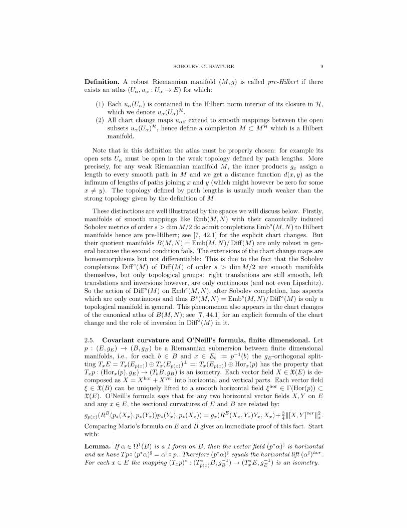
Definition. A robust Riemannian manifold (M, g) is called pre-Hilbert if thereexists an atlas (Uα, uα : Uα → E) for which:

(1) Each uα(Uα) is contained in the Hilbert norm interior of its closure in H,which we denote uα(Uα)H.

(2) All chart change maps uαβ extend to smooth mappings between the opensubsets uα(Uα)H, hence define a completion M ⊂ MH which is a Hilbertmanifold.

Note that in this definition the atlas must be properly chosen: for example itsopen sets Uα must be open in the weak topology defined by path lengths. Moreprecisely, for any weak Riemannian manifold M , the inner products gx assign alength to every smooth path in M and we get a distance function d(x, y) as theinfimum of lengths of paths joining x and y (which might however be zero for somex 6= y). The topology defined by path lengths is usually much weaker than thestrong topology given by the definition of M .

These distinctions are well illustrated by the spaces we will discuss below. Firstly,manifolds of smooth mappings like Emb(M,N) with their canonically inducedSobolev metrics of order s > dimM/2 do admit completions Embs(M,N) to Hilbertmanifolds hence are pre-Hilbert; see [7, 42.1] for the explicit chart changes. Buttheir quotient manifolds B(M,N) = Emb(M,N)/Diff(M) are only robust in gen-eral because the second condition fails. The extensions of the chart change maps arehomeomorphisms but not differentiable: This is due to the fact that the Sobolevcompletions Diffs(M) of Diff(M) of order s > dimM/2 are smooth manifoldsthemselves, but only topological groups: right translations are still smooth, lefttranslations and inversions however, are only continuous (and not even Lipschitz).So the action of Diffs(M) on Embs(M,N), after Sobolev completion, has aspectswhich are only continuous and thus Bs(M,N) = Embs(M,N)/Diffs(M) is only atopological manifold in general. This phenomenon also appears in the chart changesof the canonical atlas of B(M,N); see [7, 44.1] for an explicit formula of the chartchange and the role of inversion in Diffs(M) in it.

2.5. Covariant curvature and O’Neill’s formula, finite dimensional. Letp : (E, gE) → (B, gB) be a Riemannian submersion between finite dimensionalmanifolds, i.e., for each b ∈ B and x ∈ Eb := p−1(b) the gE-orthogonal split-ting TxE = Tx(Ep(x)) ⊕ Tx(Ep(x))

⊥ =: Tx(Ep(x)) ⊕ Horx(p) has the property thatTxp : (Horx(p), gE)→ (TbB, gB) is an isometry. Each vector field X ∈ X(E) is de-composed as X = Xhor +Xver into horizontal and vertical parts. Each vector fieldξ ∈ X(B) can be uniquely lifted to a smooth horizontal field ξhor ∈ Γ(Hor(p)) ⊂X(E). O’Neill’s formula says that for any two horizontal vector fields X,Y on Eand any x ∈ E, the sectional curvatures of E and B are related by:

gp(x)(RB(p∗(Xx), p∗(Yx))p∗(Yx), p∗(Xx)) = gx(RE(Xx, Yx)Yx, Xx)+ 3

4‖[X,Y ]ver‖2x.Comparing Mario’s formula on E and B gives an immediate proof of this fact. Startwith:

Lemma. If α ∈ Ω1(B) is a 1-form on B, then the vector field (p∗α)] is horizontaland we have Tp (p∗α)] = α] p. Therefore (p∗α)] equals the horizontal lift (α])hor.For each x ∈ E the mapping (Txp)

∗ : (T ∗p(x)B, g−1B )→ (T ∗xE, g

−1E ) is an isometry.


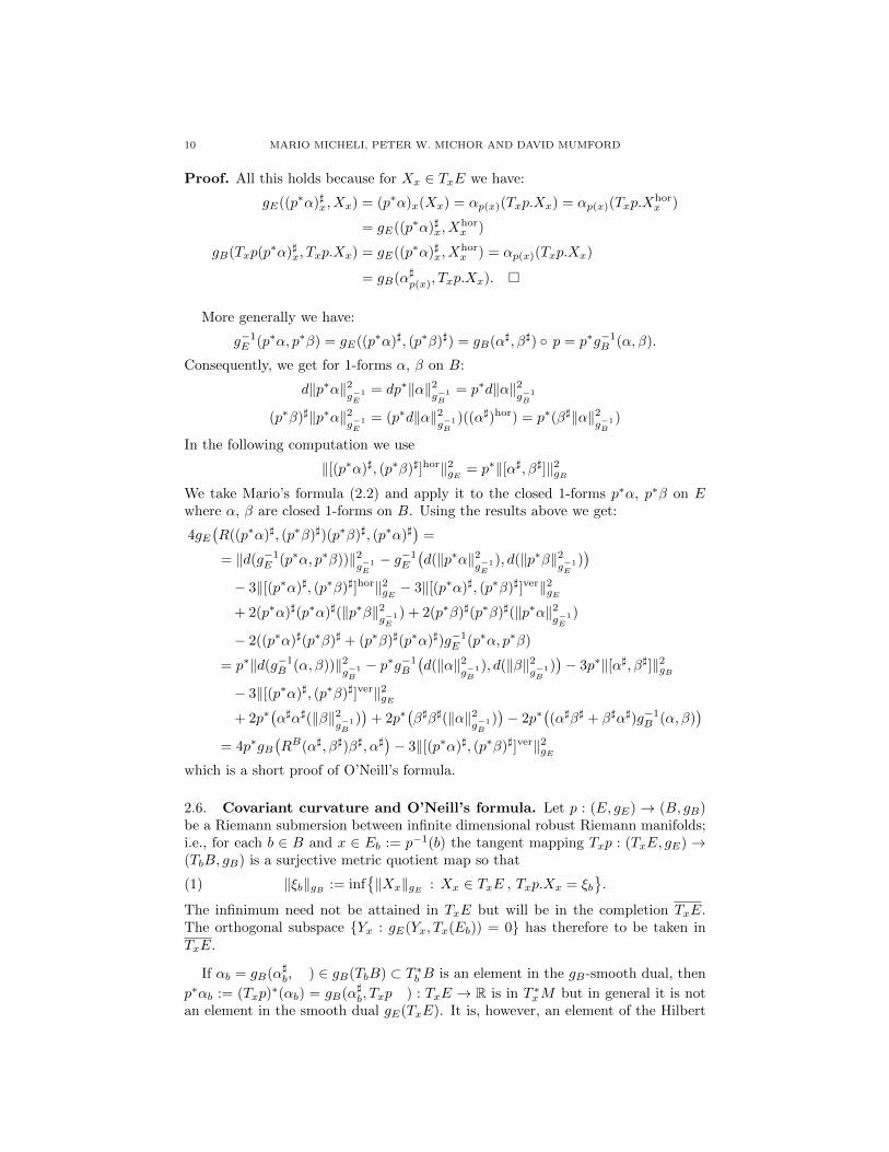
Proof. All this holds because for Xx ∈ TxE we have:

gE((p∗α)]x, Xx) = (p∗α)x(Xx) = αp(x)(Txp.Xx) = αp(x)(Txp.Xhorx )

= gE((p∗α)]x, Xhorx )

gB(Txp(p∗α)]x, Txp.Xx) = gE((p∗α)]x, X

horx ) = αp(x)(Txp.Xx)

= gB(α]p(x), Txp.Xx).

More generally we have:

g−1E (p∗α, p∗β) = gE((p∗α)], (p∗β)]) = gB(α], β]) p = p∗g−1

B (α, β).

Consequently, we get for 1-forms α, β on B:

d‖p∗α‖2g−1E

= dp∗‖α‖2g−1B

= p∗d‖α‖2g−1B

(p∗β)]‖p∗α‖2g−1E

= (p∗d‖α‖2g−1B

)((α])hor) = p∗(β]‖α‖2g−1B

)

In the following computation we use

‖[(p∗α)], (p∗β)]]hor‖2gE = p∗‖[α], β]]‖2gBWe take Mario’s formula (2.2) and apply it to the closed 1-forms p∗α, p∗β on Ewhere α, β are closed 1-forms on B. Using the results above we get:

4gE(R((p∗α)], (p∗β)])(p∗β)], (p∗α)]

)=

= ‖d(g−1E (p∗α, p∗β))‖2

g−1E

− g−1E

(d(‖p∗α‖2

g−1E

), d(‖p∗β‖2g−1E

))

− 3‖[(p∗α)], (p∗β)]]hor‖2gE − 3‖[(p∗α)], (p∗β)]]ver‖2gE+ 2(p∗α)](p∗α)](‖p∗β‖2

g−1E

) + 2(p∗β)](p∗β)](‖p∗α‖2g−1E

)

− 2((p∗α)](p∗β)] + (p∗β)](p∗α)])g−1E (p∗α, p∗β)

= p∗‖d(g−1B (α, β))‖2

g−1B

− p∗g−1B

(d(‖α‖2

g−1B

), d(‖β‖2g−1B

))− 3p∗‖[α], β]]‖2gB

− 3‖[(p∗α)], (p∗β)]]ver‖2gE+ 2p∗

(α]α](‖β‖2

g−1B

))

+ 2p∗(β]β](‖α‖2

g−1B

))− 2p∗

((α]β] + β]α])g−1

B (α, β))

= 4p∗gB(RB(α], β])β], α]

)− 3‖[(p∗α)], (p∗β)]]ver‖2gE

which is a short proof of O’Neill’s formula.

2.6. Covariant curvature and O’Neill’s formula. Let p : (E, gE) → (B, gB)be a Riemann submersion between infinite dimensional robust Riemann manifolds;i.e., for each b ∈ B and x ∈ Eb := p−1(b) the tangent mapping Txp : (TxE, gE) →(TbB, gB) is a surjective metric quotient map so that

(1) ‖ξb‖gB := inf‖Xx‖gE : Xx ∈ TxE , Txp.Xx = ξb

.

The infinimum need not be attained in TxE but will be in the completion TxE.The orthogonal subspace Yx : gE(Yx, Tx(Eb)) = 0 has therefore to be taken inTxE.

If αb = gB(α]b, ) ∈ gB(TbB) ⊂ T ∗b B is an element in the gB-smooth dual, then

p∗αb := (Txp)∗(αb) = gB(α]b, Txp ) : TxE → R is in T ∗xM but in general it is not

an element in the smooth dual gE(TxE). It is, however, an element of the Hilbert

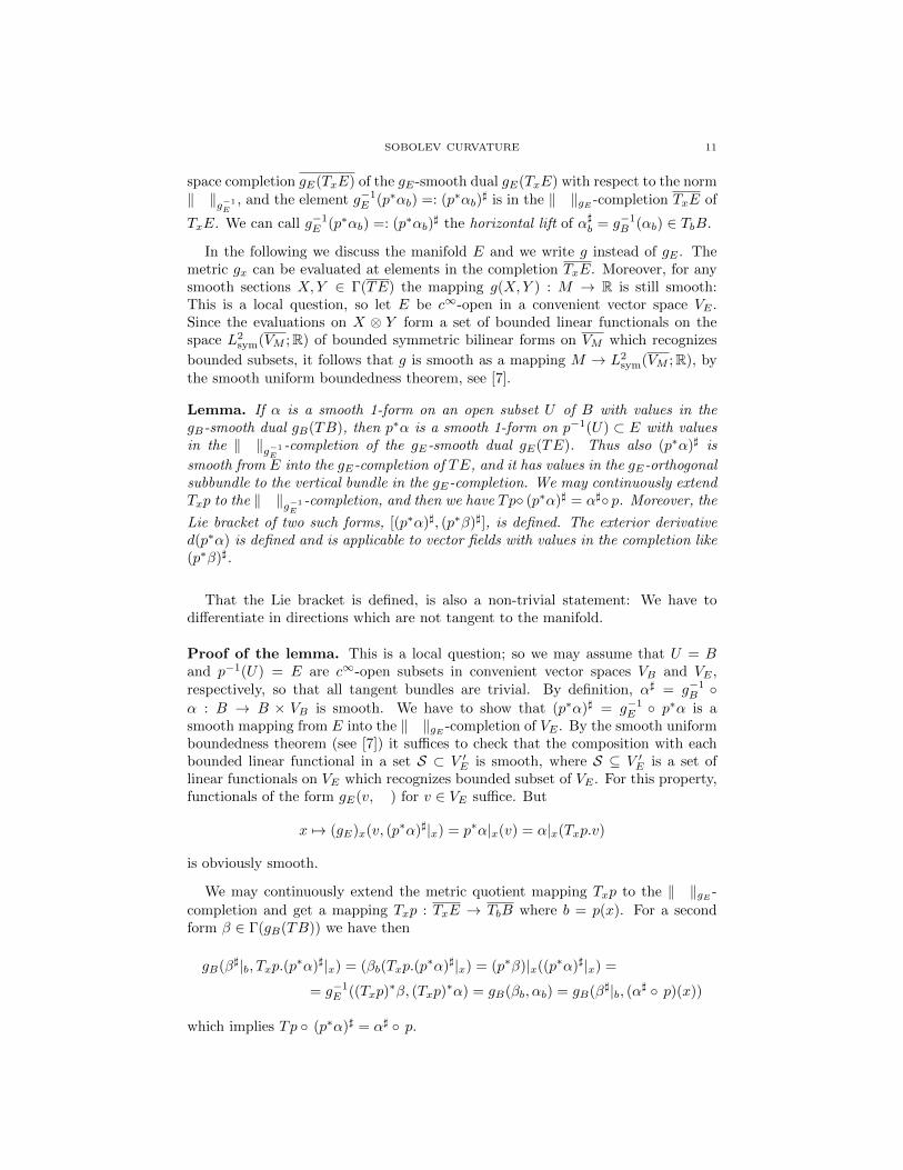
SOBOLEV CURVATURE 11

space completion gE(TxE) of the gE-smooth dual gE(TxE) with respect to the norm‖ ‖g−1

E, and the element g−1

E (p∗αb) =: (p∗αb)] is in the ‖ ‖gE -completion TxE of

TxE. We can call g−1E (p∗αb) =: (p∗αb)

] the horizontal lift of α]b = g−1B (αb) ∈ TbB.

In the following we discuss the manifold E and we write g instead of gE . Themetric gx can be evaluated at elements in the completion TxE. Moreover, for anysmooth sections X,Y ∈ Γ(TE) the mapping g(X,Y ) : M → R is still smooth:This is a local question, so let E be c∞-open in a convenient vector space VE .Since the evaluations on X ⊗ Y form a set of bounded linear functionals on thespace L2

sym(VM ;R) of bounded symmetric bilinear forms on VM which recognizes

bounded subsets, it follows that g is smooth as a mapping M → L2sym(VM ;R), by

the smooth uniform boundedness theorem, see [7].

Lemma. If α is a smooth 1-form on an open subset U of B with values in thegB-smooth dual gB(TB), then p∗α is a smooth 1-form on p−1(U) ⊂ E with valuesin the ‖ ‖g−1

E-completion of the gE-smooth dual gE(TE). Thus also (p∗α)] is

smooth from E into the gE-completion of TE, and it has values in the gE-orthogonalsubbundle to the vertical bundle in the gE-completion. We may continuously extendTxp to the ‖ ‖g−1

E-completion, and then we have Tp (p∗α)] = α] p. Moreover, the

Lie bracket of two such forms, [(p∗α)], (p∗β)]], is defined. The exterior derivatived(p∗α) is defined and is applicable to vector fields with values in the completion like(p∗β)].

That the Lie bracket is defined, is also a non-trivial statement: We have todifferentiate in directions which are not tangent to the manifold.

Proof of the lemma. This is a local question; so we may assume that U = Band p−1(U) = E are c∞-open subsets in convenient vector spaces VB and VE ,respectively, so that all tangent bundles are trivial. By definition, α] = g−1

B α : B → B × VB is smooth. We have to show that (p∗α)] = g−1

E p∗α is asmooth mapping from E into the ‖ ‖gE -completion of VE . By the smooth uniformboundedness theorem (see [7]) it suffices to check that the composition with eachbounded linear functional in a set S ⊂ V ′E is smooth, where S ⊆ V ′E is a set oflinear functionals on VE which recognizes bounded subset of VE . For this property,functionals of the form gE(v, ) for v ∈ VE suffice. But

x 7→ (gE)x(v, (p∗α)]|x) = p∗α|x(v) = α|x(Txp.v)

is obviously smooth.

We may continuously extend the metric quotient mapping Txp to the ‖ ‖gE -

completion and get a mapping Txp : TxE → TbB where b = p(x). For a secondform β ∈ Γ(gB(TB)) we have then

gB(β]|b, Txp.(p∗α)]|x) = (βb(Txp.(p∗α)]|x) = (p∗β)|x((p∗α)]|x) =

= g−1E ((Txp)

∗β, (Txp)∗α) = gB(βb, αb) = gB(β]|b, (α] p)(x))

which implies Tp (p∗α)] = α] p.


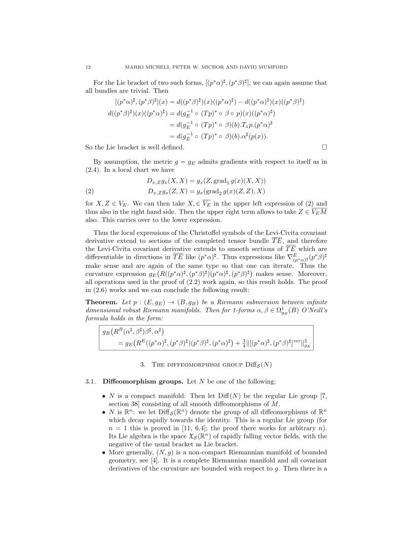
For the Lie bracket of two such forms, [(p∗α)], (p∗β)]], we can again assume thatall bundles are trivial. Then

[(p∗α)], (p∗β)]](x) = d((p∗β)])(x)((p∗α)])− d((p∗α)])(x)((p∗β)])

d((p∗β)])(x)((p∗α)]) = d(g−1E (Tp)∗ β p)(x)((p∗α)])

= d(g−1E (Tp)∗ β)(b).Txp.(p

∗α)]

= d(g−1E (Tp)∗ β)(b).α](p(x)).

So the Lie bracket is well defined.

By assumption, the metric g = gE admits gradients with respect to itself as in(2.4). In a local chart we have

Dx,Zgx(X,X) = gx(Z, grad1 g(x)(X,X))

Dx,Zgx(Z,X) = gx(grad2 g(x)(Z,Z), X)(2)

for X,Z ∈ VE . We can then take X,∈ VE in the upper left expression of (2) andthus also in the right hand side. Then the upper right term allows to take Z ∈ VEMalso. This carries over to the lower expression.

Thus the local expressions of the Christoffel symbols of the Levi-Civita covariantderivative extend to sections of the completed tensor bundle TE, and thereforethe Levi-Civita covariant derivative extends to smooth sections of TE which aredifferentiable in directions in TE like (p∗α)]. Thus expressions like ∇E(p∗α)](p

∗β)]

make sense and are again of the same type so that one can iterate. Thus thecurvature expression gE

(R((p∗α)], (p∗β)])(p∗α)], (p∗β)]

)makes sense. Moreover,

all operations used in the proof of (2.2) work again, so this result holds. The proofin (2.6) works and we can conclude the following result:

Theorem. Let p : (E, gE) → (B, gB) be a Riemann submersion between infinitedimensional robust Riemann manifolds. Then for 1-forms α, β ∈ Ω1

gB (B) O’Neill’sformula holds in the form:

gB(RB(α], β])β], α]

)= gE

(RE((p∗α)], (p∗β)])(p∗β)], (p∗α)]

)+ 3

4‖[(p∗α)], (p∗β)]]ver‖2gE

3. The diffeomorphism group DiffS(N)

3.1. Diffeomorphism groups. Let N be one of the following:

• N is a compact manifold: Then let Diff(N) be the regular Lie group [7,section 38] consisting of all smooth diffeomorphisms of M .• N is Rn: we let DiffS(Rn) denote the group of all diffeomorphisms of Rn

which decay rapidly towards the identity. This is a regular Lie group (forn = 1 this is proved in [11, 6.4]; the proof there works for arbitrary n).Its Lie algebra is the space XS(Rn) of rapidly falling vector fields, with thenegative of the usual bracket as Lie bracket.• More generally, (N, g) is a non-compact Riemannian manifold of bounded

geometry, see [4]. It is a complete Riemannian manifold and all covariantderivatives of the curvature are bounded with respect to g. Then there is a


well developed theory of Sobolev spaces on N ; let H∞ denote the intersec-tion of all Sobolev spaces which consists of smooth functions (or sections).Even on N = R the space H∞ is strictly larger than the subspace S ofall rapidly decreasing functions (or sections) which can be defined by thecondition that the Riemannian norm of all iterated covariant derivativesdecreases faster than the inverse of any power of the Riemannian distance.There is nearly no information available on the space S for a general Rie-mannian manifold of bounded geometry. For the following we let S denoteeither H∞ or the space of rapidly decreasing functions. We let DiffS(N)denote the group of all diffeomorphisms which decay rapidly towards theidentity (or differ from the identity by H∞). It is a regular Lie group withLie algebra the space XS(N) of rapidly decreasing vector fields with thenegative of the usual bracket. In [11, 6.4] this was proved for N = R, butthe same proof should work for the general case discussed here.

In general, we need to impose some boundary conditions near infinity for groupsof diffeomorphisms on a non-compact manifold N : The full group Diff(N) of alldiffeomorphisms with its natural compact C∞ topology is not locally contractible,so it does not admit any atlas of open charts.

For uniformity of notation, we shall denote by DiffS(N) any of these regularLie groups. Its Lie algebra is denoted by XS(N) in each of these cases, with thenegative of the usual bracket as Lie bracket. We also shall denote by O = C∞ ∩S ′the space of smooth functions in the dual space S ′ (to be specific, this is the spaceOM in the sense of Laurent Schwartz, if N = Rn).

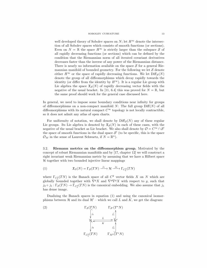
3.2. Riemann metrics on the diffeomorphism group. Motivated by theconcept of robust Riemannian manifolds and by [17, chapter 12] we will construct aright invariant weak Riemannian metric by assuming that we have a Hilbert spaceH together with two bounded injective linear mappings

(1) XS(N) = ΓS(TN)j1−−−→ H j2−−−→ ΓC2

b(TN)

where ΓC2b(TN) is the Banach space of all C2 vector fields X on N which are

globally bounded together with ∇gX and ∇g∇gX with respect to g, such thatj2 j1 : ΓS(TN)→ ΓC2

b(TN) is the canonical embedding. We also assume that j1

has dense image.

Dualizing the Banach spaces in equation (1) and using the canonical isomor-phisms between H and its dual H′ – which we call L and K, we get the diagram:

(2) ΓS(TN) _

j1

ΓS′(T∗N)

H _j2

L // H′?

j′1

OO

Koo

ΓC2b(TN) ΓM2(T ∗N)

?

j′2

OO


Here we have written ΓS′(T∗N) for the dual of the space of smooth vector fields

ΓS(TN) = XS(N). We call these 1-co-currents as 1-currents are elements in thedual of ΓS(T ∗N). It contains smooth measure valued cotangent vectors on N(which we will write as ΓS(T ∗N ⊗ vol(N))) and as well as the bigger subspace ofsecond derivatives of finite measure valued 1-forms on N which we have written asΓM2(T ∗N) and which is part of the dual of ΓC2

b(TN). In what follows, we will have

many momentum variables with values in these spaces.

The restriction of L to XS(N) via j1 gives us a positive definite weak innerproduct on XS(N) which may be defined by a distribution valued kernel – whichwe also write as L:

〈 , 〉L : XS(N)× XS(N)→ R, defined by

〈X,Y 〉L = 〈j1X, j1Y 〉H =

∫∫N×N

(X(y1)⊗ Y (y2), L(y1, y2)),

where L ∈ ΓS′(pr∗1(T ∗N)⊗ pr∗2(T ∗N))

Extending this weak inner product right invariantly over DiffS(N), we get a robustweak Riemannian manifold in the sense of 2.4.

In the case (called the standard case below) that N = Rn and that

〈X,Y 〉L =

∫Rn〈(1−A∆)lX,Y 〉 dx

we have

L(x, y) =( 1

(2π)n

∫ξ∈Rn

ei〈ξ,x−y〉(1 +A|ξ|2)ldξ) n∑i=1

(dui|x ⊗ dx)⊗ (dui|y ⊗ dy)

where dξ, dx and dy denote Lebesque measure, and where (ui) are linear coordinateson Rn. Here H is the space of Sobolev H l vector fields on N .

Note that given an operator L with appropriate properties we can reconstructthe Hilbert space H with the two bounded injective mappings j1, j2.

Construction of the reproducing kernel K: The inverse map K is even nicer as itis given by a C2 tensor, the reproducing kernel. To see this, note that ΓM2(T ∗N)contains the measures supported at one point x defined by an element αx ∈ T ∗xN .Then j2(K(j′2(αx))) is given by a C2 vector field Kαx on Nwhich satisfies:

(3) 〈Kαx , X〉H = αx(j2X)(x) for all X ∈ H, αx ∈ T ∗xN.The map αx 7→ Kαx is weakly C2

b , thus by [7, theorem 12.8] this mapping is strongly

Lip1 (i.e., differentiable and the derivative is locally Lipschitz, for the norm on H).Since evy K : T ∗xN 3 αx 7→ Kαx(y) ∈ TyN is linear we get a correspondingelement K(x, y) ∈ L(T ∗xN,TyN) = TxN ⊗ TyN with K(y, x)(αx) = Kαx(y).

Using (3) twice we have (omitting j2)

βy.K(y, x)(αx) = 〈K( , x)(αx),K( , y)(βy)〉H = αx.K(x, y)(βy)

so that:

• K(x, y)> = K(y, x) : T ∗yN → TxN ,• K ∈ ΓC2

b(pr1

∗ TN ⊗ pr∗2 TN).


Moreover the operator K defined directly by integration

K : ΓM2(T ∗N)→ ΓC2b(TN)

K(α)(y2) =

∫y1∈N

(K(y1, y2), α(y1)).

is the same as the inverse K to L. In fact, by definition, they agree on sectionsin ΓC2(T ∗M) with finite support and these are weakly dense. Hence they agreeeverywhere.

We will sometimes use the abbreviations 〈α|K|, |K|β〉 and 〈α|K|β〉 for the con-traction of the vector values of K in its first and second variable against 1-forms αand β. Often these are measure valued 1-forms so after contracting, there remainsa measure in that variable which can be integrated.

Thus the C2 tensor K determines L and hence H and hence the whole metricon DiffS(N). It is tempting to start with the tensor K, assuming it is symmetricand positive definite in a suitable sense. But rather subtle conditions on K arerequired in order that its inverse L is defined on all infinitely differentiable vector

fields. For example, if N = R, the Gaussian kernel K(x, y) = e−|x−y|2

does notgive such an L.

In the standard case we have

K(x, y) = Kl(x− y)

n∑i=1

∂

∂xi⊗ ∂

∂yi,

Kl(x) =1

(2π)n

∫ξ∈Rn

ei〈ξ,x〉

(1 +A|ξ|2)ldξ

where Kl is given by a classical Bessel function of differentiability class C2l.

3.3. The zero compressibility limit. Although the family of metrics abovedoes not include the case originally studied by Arnold – the L2 metric on volumepreserving diffeomorphisms – they do include metrics which have this case as alimit. Taking N = Rn and starting with the standard Sobolev metric, we can adda divergence term with a coefficient B:

〈X,Y 〉L =

∫Rn

(〈(1−A∆)lX,Y 〉+B.div(X)div(Y )

)dx

Note that as B approaches ∞, the geodesics will tend to lie on the cosets withrespect to the subgroup of volume preserving diffeomorphisms. And when, in ad-dition, A approaches zero, we get the simple L2 metric used by Arnold. Thissuggests that, as in the so-called ‘zero-viscosity limit’, we should be able to con-struct geodesics in Arnold’s metric, i.e. solutions of Euler’s equation, as limits ofgeodesics for this larger family of metrics on the full group.

The resulting kernels L and K are no longer diagonal. To L, we must add

B

n∑i=1

n∑j=1

( 1

(2π)n

∫ξ∈Rn

ei〈ξ,x−y〉ξi.ξjdξ)

(dui|x ⊗ dx)⊗ (duj |y ⊗ dy).


It can be checked that the corresponding kernel K will have the form

K(x, y) = K0(x− y)

n∑i=1

∂

∂xi⊗ ∂

∂yi+

n∑i=1

n∑j=1

(KB),ij(x− y)∂

∂xi⊗ ∂

∂yj

where K0 is the kernel as above for the standard norm of order l and KB is a secondradially symmetric kernel on Rn depending on B.

3.4. The geodesic equation. According to [2], the geodesic equation on anyLie group G with a right-invariant metric is given as follows. Let g(t) be a path in

G and let u(t) = g(t).g(t)−1 = T (µg(t)−1

)g(t) be the right logarithmic derivative, apath in its Lie algebra g. Here µg : G→ G is right translation by g. Then g(t) is ageodesic if and only if

∂tu = − ad>u u.

where the transposed ad>X is the adjoint of adX : g→ g with respect to the metricon g.

In our case the Lie algebra of DiffS(N) is the space XS(N) of all rapidly decreas-ing smooth vector fields with Lie bracket (we write adX Y ) the negative of the usualLie bracket adX Y = −[X,Y ]). Then a smooth curve t 7→ ϕ(t) of diffeomorphismsis a geodesic for the right invariant weak Riemannian metric on DiffS(N) inducedby the weak inner product 〈 , 〉L on XS(N) if and only if

∂tu = − ad>u u.

as above. Here the time dependent vector field u is now given by ∂tϕ(t) = u(t)ϕ(t),

and the transposed ad>X is given by

〈ad>X Y, Z〉L = 〈Y, adX Z〉L = −〈Y, [X,Z]〉L.

The inner product is weak; existence of ad>X implies condition (1) for robustnessof the weak Riemannian manifold (DiffS(N), 〈 , 〉L); it is equivalent to the factthat the dual mapping ad∗X : XS(N)′ → XS(N)′ maps the smooth dual L(XS(N))

to itself. We also have L ad>X = ad∗X L. Using Lie derivatives, the computationof ad∗X is especially simple. Namely, for any section ω of T ∗N ⊗ vol and vectorfields ξ, η ∈ XS(N), we have:∫

N

(ω, [ξ, η]) =

∫N

(ω,Lξ(η)) = −∫N

(Lξ(ω), η),

hence ad∗ξ(ω) = +Lξ(ω). Thus the Hamiltonian version of the geodesic equationon the smooth dual L(XS(N)) ⊂ ΓC2(T ∗N ⊗ vol) becomes

∂tα = − ad∗K(α) α = −LK(α)α,

or, keeping track of everything,

(1)

∂tϕ = u ϕ,∂tα = −Luα

u = K(α) = α], α = L(u) = u[.

One can also derive the geodesic equation from the conserved momentum mappingJ : T DiffS(N)→ XS(N)′ given by J(g,X) = L Ad(g)>X where Ad(g)X = Tg X g−1. This means that Ad(g(t))u(t) is conserved and 0 = ∂t Ad(g(t))u(t) leads


quickly to the geodesic equation. It is remarkable that the momentum mappingexists if and only if (DiffS(N), 〈 , 〉L) is a robust weak Riemannian manifold.

4. The differentiable Chow manifold (alias the non-linearGrassmannian)

4.1. The differentiable Chow manifold as a homogeneous space forDiffS(N) and the induced weak Riemannian metric. Let M be a compactmanifold with dim(M) < dim(N). The space of submanifolds of N diffeomorphicto M will be called B(M,N). In the case m = 0 and N = RD, i.e. M is a finite setof, say p, points in Euclidean D-space, the space B(M,N) is what we called thespace of landmark points Lp(RD) in our earlier paper [9].

B(M,N) can be viewed as a quotient of DiffS(N). If we fix a base submanifoldF0 ⊂ N diffeomorphic to M , then we get a map of DiffS(N) into B(M,N) byϕ 7→ ϕ(F0). The image will be an open subset B0(M,N) of B(M,N) which is thequotient of DiffS(N) by the subgroup of diffeomorphisms which map F0 to itself.We will study B(M,N) using this approach and without further comment replacethe full space B(M,N) by this component B0(M,N).

The normal bundle to F ⊂ N may be defined as TB⊥ ⊂ TN |B , with the helpof an auxiliary Riemann metric on N . But we want to avoid this auxiliary metric,so we shall define the normal bundle as the quotient Nor(F ) := TN |F /TF overF . Then its dual bundle, the conormal bundle, is Nor∗(F ) = Annihilator(TF ) ⊂T ∗N |F , a sub-bundle not a quotient. The tangent space TFB(M,N)to B(M,N) atF can be identified with the space of all smooth sections ΓS(Nor(F )) of the normalbundle.

A simple way to construct local coordinates on B(M,N) near a point F ∈B(M,N) is to trivialize a neighborhood of F ⊂ N . To be precise, assume we havea tubular neighborhood, i.e., an isomorphism Φ:

B(M,N) Nor(F )∪ ∪UB

Φ−→ UN∪ ∪F = 0-section

from an open neighborhood UB of F in N to an open neighborhood UN of the0-section in the normal bundle Nor(F ). Assume moreover that Φ is the identity onF and its normal derivative along F induces the identity map on Nor(F ). The mapΦ induces a local projection π : UB → F and partial linear structure in the fibres ofthis projection. Then we get an open set UΦ ⊂ B(M,N) consisting of submanifoldsF ′ ⊂ UB which intersect the fibres of π normally in exactly one point. Under Φthese submanifolds are all given by smooth sections of Nor(F ) which lie in UN . Ifwe call this set of sections UΓ we have a chart:

B(M,N) ⊃ UΦ∼= UΓ ⊂ ΓS(Nor(F ))


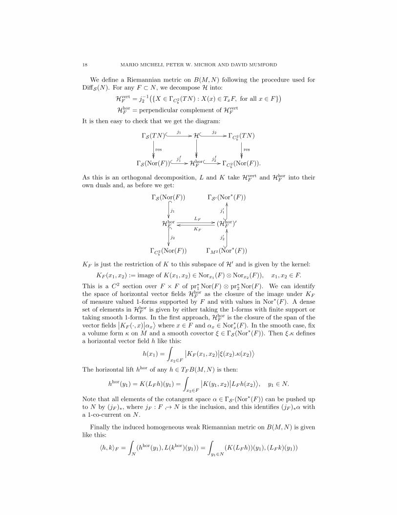
We define a Riemannian metric on B(M,N) following the procedure used forDiffS(N). For any F ⊂ N , we decompose H into:

HvertF = j−1

2

(X ∈ ΓC2

b(TN) : X(x) ∈ TxF, for all x ∈ F

)HhorF = perpendicular complement of Hvert

F

It is then easy to check that we get the diagram:

ΓS(TN) j1 //

res

H j2 //

ΓC2b(TN)

res

ΓS(Nor(F ))

jf1 // Hhor

F jf2 // ΓC2

b(Nor(F )).

As this is an orthogonal decomposition, L and K take HvertF and Hhor

F into theirown duals and, as before we get:

ΓS(Nor(F )) _

j1

ΓS′(Nor∗(F ))

HhorF _

j2

LF // (HhorF )′?

j′1

OO

KF

oo

ΓC2b(Nor(F )) ΓM2(Nor∗(F ))

?

j′2

OO

KF is just the restriction of K to this subspace of H′ and is given by the kernel:

KF (x1, x2) := image of K(x1, x2) ∈ Norx1(F )⊗Norx2

(F )), x1, x2 ∈ F.This is a C2 section over F × F of pr∗1 Nor(F ) ⊗ pr∗2 Nor(F ). We can identifythe space of horizontal vector fields Hhor

F as the closure of the image under KF

of measure valued 1-forms supported by F and with values in Nor∗(F ). A denseset of elements in Hhor

F is given by either taking the 1-forms with finite support ortaking smooth 1-forms. In the first approach, Hhor

F is the closure of the span of thevector fields

∣∣KF (·, x)∣∣αx⟩ where x ∈ F and αx ∈ Nor∗x(F ). In the smooth case, fix

a volume form κ on M and a smooth covector ξ ∈ ΓS(Nor∗(F )). Then ξ.κ definesa horizontal vector field h like this:

h(x1) =

∫x2∈F

∣∣KF (x1, x2)∣∣ξ(x2).κ(x2)

⟩The horizontal lift hhor of any h ∈ TFB(M,N) is then:

hhor(y1) = K(LFh)(y1) =

∫x2∈F

∣∣K(y1, x2)∣∣LFh(x2)

⟩, y1 ∈ N.

Note that all elements of the cotangent space α ∈ ΓS′(Nor∗(F )) can be pushed upto N by (jF )∗, where jF : F → N is the inclusion, and this identifies (jF )∗α witha 1-co-current on N .

Finally the induced homogeneous weak Riemannian metric on B(M,N) is givenlike this:

〈h, k〉F =

∫N

(hhor(y1), L(khor)(y1)) =

∫y1∈N

(K(LFh))(y1), (LF k)(y1))


=

∫(y1,y2)∈N×N

(K(y1, y2), (LFh)(y1)⊗ (LF k)(y2))

=

∫(x1,x1)∈F×F

⟨LFh(x1)

∣∣KF (x1, x2)∣∣LFh(x2)

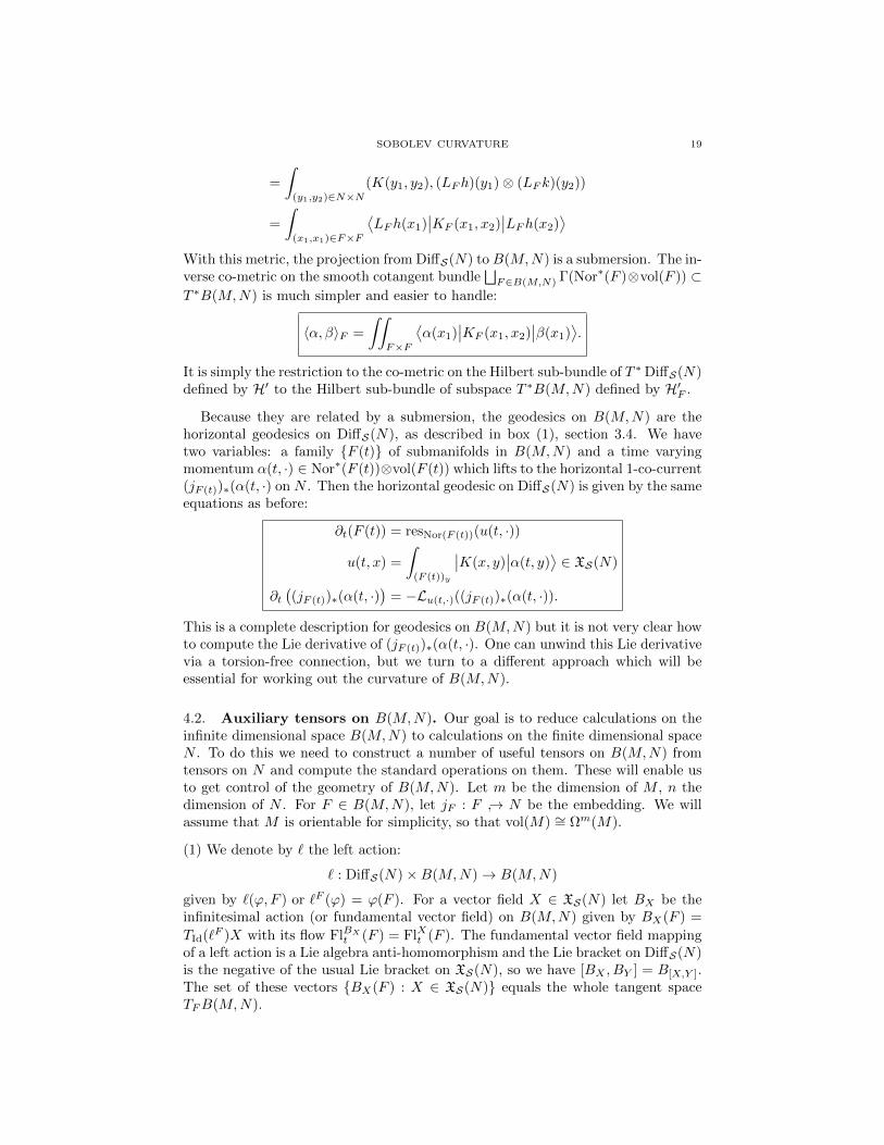
⟩With this metric, the projection from DiffS(N) toB(M,N) is a submersion. The in-verse co-metric on the smooth cotangent bundle

⊔F∈B(M,N) Γ(Nor∗(F )⊗vol(F )) ⊂

T ∗B(M,N) is much simpler and easier to handle:

〈α, β〉F =

∫∫F×F

⟨α(x1)

∣∣KF (x1, x2)∣∣β(x1)

⟩.

It is simply the restriction to the co-metric on the Hilbert sub-bundle of T ∗DiffS(N)defined by H′ to the Hilbert sub-bundle of subspace T ∗B(M,N) defined by H′F .

Because they are related by a submersion, the geodesics on B(M,N) are thehorizontal geodesics on DiffS(N), as described in box (1), section 3.4. We havetwo variables: a family F (t) of submanifolds in B(M,N) and a time varyingmomentum α(t, ·) ∈ Nor∗(F (t))⊗vol(F (t)) which lifts to the horizontal 1-co-current(jF (t))∗(α(t, ·) on N . Then the horizontal geodesic on DiffS(N) is given by the sameequations as before:

∂t(F (t)) = resNor(F (t))(u(t, ·))

u(t, x) =

∫(F (t))y

∣∣K(x, y)∣∣α(t, y)

⟩∈ XS(N)

∂t((jF (t))∗(α(t, ·)

)= −Lu(t,·)((jF (t))∗(α(t, ·)).

This is a complete description for geodesics on B(M,N) but it is not very clear howto compute the Lie derivative of (jF (t))∗(α(t, ·). One can unwind this Lie derivativevia a torsion-free connection, but we turn to a different approach which will beessential for working out the curvature of B(M,N).

4.2. Auxiliary tensors on B(M,N). Our goal is to reduce calculations on theinfinite dimensional space B(M,N) to calculations on the finite dimensional spaceN . To do this we need to construct a number of useful tensors on B(M,N) fromtensors on N and compute the standard operations on them. These will enable usto get control of the geometry of B(M,N). Let m be the dimension of M , n thedimension of N . For F ∈ B(M,N), let jF : F → N be the embedding. We willassume that M is orientable for simplicity, so that vol(M) ∼= Ωm(M).

(1) We denote by ` the left action:

` : DiffS(N)×B(M,N)→ B(M,N)

given by `(ϕ, F ) or `F (ϕ) = ϕ(F ). For a vector field X ∈ XS(N) let BX be theinfinitesimal action (or fundamental vector field) on B(M,N) given by BX(F ) =

TId(`F )X with its flow FlBXt (F ) = FlXt (F ). The fundamental vector field mappingof a left action is a Lie algebra anti-homomorphism and the Lie bracket on DiffS(N)is the negative of the usual Lie bracket on XS(N), so we have [BX , BY ] = B[X,Y ].The set of these vectors BX(F ) : X ∈ XS(N) equals the whole tangent spaceTFB(M,N).


(2) Note that B(M,N) is naturally submanifold of the vector space of m-currentson N :

B(M,N) → ΩmS (N)′ = ΓS′(ΛmTN), via F 7→

(ω 7→

∫F

ω

).

Any α ∈ Ωm(N) is a linear coordinate on ΓS′(ΛmTN) and this restricts to the

function Bα ∈ C∞(B(M,N),R) given by Bα(F ) =∫Fα. If α = dβ for β ∈

Ωm−1(N) then

Bα(F ) = Bdβ(F ) =

∫F

j∗F dβ =

∫F

dj∗Fβ = 0

by Stokes’ theorem.

For α ∈ Ωm(N) and X ∈ XS(N) we can evaluate the vector field BX on thefunction Bα:

BX(Bα)(F ) = dBα(BX)(F ) = ∂t|0Bα(FlXt (F )) =

∫F

j∗FLXα = BLX(α)(F )

as well as =

∫F

j∗F (iXdα+ diXα) =

∫F

j∗F iXdα = BiX(dα)(F )

If X ∈ XS(N) is tangent to F along F then BX(Bα)(F ) =∫FLX|F j∗Fα = 0.

More generally, a pm-form α on Nk defines a function B(p)α on B(M,N) by

B(p)α (F ) =

∫Fpα. Using this for p = 2, we find that for any two m-forms α, β on

N , the inner product of Bα and Bβ is given by:

g−1B (Bα, Bβ) = B

(2)〈α|K|β〉.

(3) For α ∈ Ωm+k(N) we denote by Bα the k-form in Ωk(B(M,N)) given by theskew-symmetric multi-linear form:

(Bα)F (BX1(F ), . . . , BXk(F )) =

∫F

jF∗(iX1∧···∧Xkα).

This is well defined: If one of the Xi is tangential to F at a point x ∈ F then jF∗

pulls back the resulting m-form to 0 at x.

Note that any smooth cotangent vector a to F ∈ B(M,N) is equal to Bα(F )for some closed (m + 1)-form α. Smooth cotangent vectors at F are elements ofΓS(F,Nor∗(F )⊗ Ωm(F )). Fix a nowhere zero global section κ of Ωm(F ). Then a

κis the differential of a unique function f on the normal bundle to F which is linearon each fibre. Let ϕ be a local isomorphism from a neighborhood of F in N to aneighborhood of the 0-section in this normal bundle and let ρ be a function on thenormal bundle which is one near the 0-section and has support in this neighborhood.Take α = d(f.κ ϕ) (extended by zero). It’s easy to see that this does it.

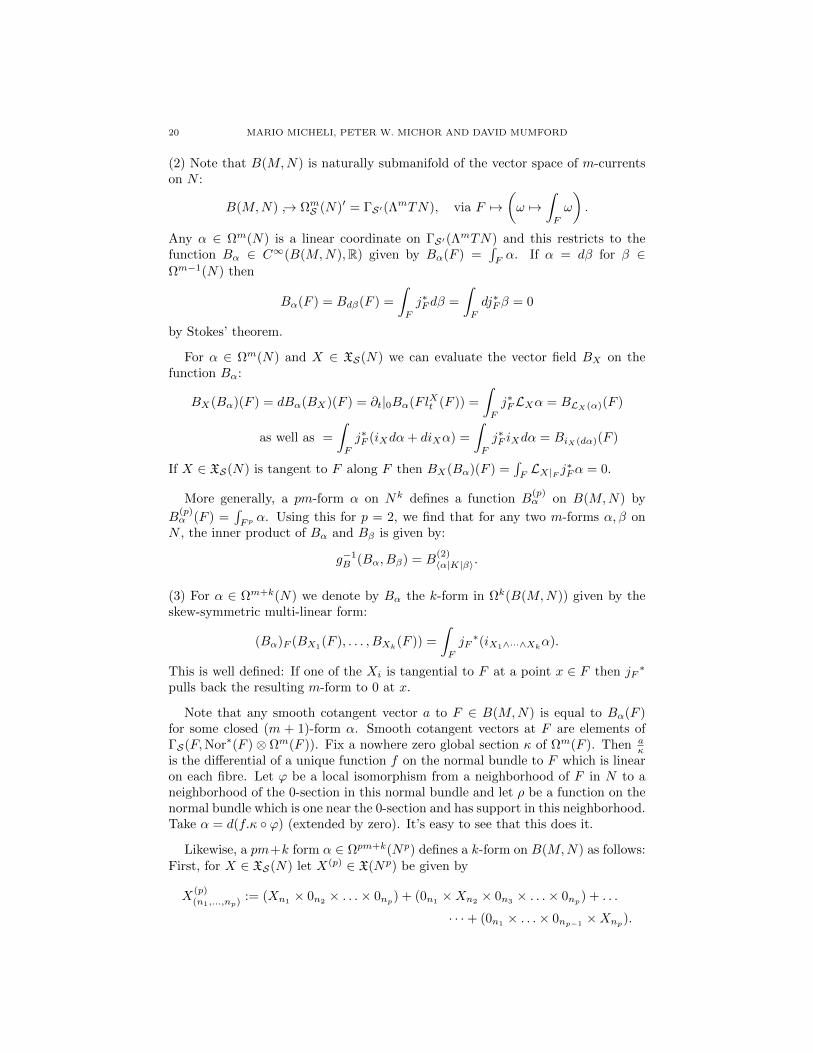
Likewise, a pm+k form α ∈ Ωpm+k(Np) defines a k-form on B(M,N) as follows:First, for X ∈ XS(N) let X(p) ∈ X(Np) be given by

X(p)(n1,...,np) := (Xn1 × 0n2 × . . .× 0np) + (0n1 ×Xn2 × 0n3 × . . .× 0np) + . . .

· · ·+ (0n1× . . .× 0np−1

×Xnp).


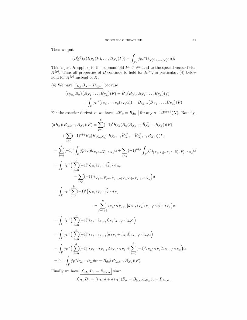
Then we put

(B(p)α )F (BX1(F ), . . . , BXk(F )) =

∫FpjFp∗(i

X(p)1 ∧···∧X

(p)k

α).

This is just B applied to the submanifold F p ⊂ Np and to the special vector fieldsX(p). Thus all properties of B continue to hold for B(p); in particular, (4) belowhold for X(p) instead of X.

(4) We have iBXBα = BiXα because(iBX1

Bα)(BX2

, . . . , BXk)(F ) = Bα

(BX1

, BX2, . . . , BXk

)(f)

=

∫F

jF∗(iXk . . . iX2

(iX1α))

= BiX1α

(BX2

, . . . , BXk)(F )

For the exterior derivative we have dBα = Bdα for any α ∈ Ωm+k(N). Namely,

(dBα)(BX0, ··, BXk)(F ) =

k∑i=0

(−1)iBXi(Bα(BX0, ··, BXi , ··, BXk))(F )

+∑i<j

(−1)i+jBα(B[Xi,Xj ], BX0 , ··, BXi , · · BXj , ··, BXk))(F )

=

k∑i=0

(−1)i∫F

j∗F iXidiX0∧··Xi··∧Xkα+∑i<j

(−1)i+j∫F

j∗F i[Xi,Xj ]∧X0∧··Xi··Xj ··∧Xkα

=

∫F

jF∗( k∑i=0

(−1)iLXiiXk · ·iXi · ·iX0

−∑i<j

(−1)iiX0∧··Xi··∧Xj−1∧[Xi,Xj ]∧Xj+1··∧Xk

)α

=

∫F

jF∗

k∑i=0

(−1)i(LXiiXk· ·iXi· ·iX0

−k∑

j=i+1

iXk· ·iXj+1 [LXi , iXj ] iXj−1· ·iXi· ·iX0

)α

=

∫F

jF∗( k∑i=0

(−1)iiXk· ·iXi+1LXiiXi−1

· ·iX0α)

=

∫F

jF∗( k∑i=0

(−1)iiXk· ·iXi+1(d iXi + iXid)iXi−1· ·iX0α)

=

∫F

jF∗( k∑i=0

(−1)iiXk · ·iXi+1d iXi · ·iX0

+

k∑i=0

(−1)iiXk· ·iXid iXi−1· ·iX0

)α

= 0 +

∫F

jF∗iXk · ·iX0

dα = Bdα(BX0, ··, BXk)(F )

Finally we have LBXBα = BLXα since

LBXBα = (iBX d+ d iBX )Bα = B(iXd+diX)α = BLXα.


Note that these identities generalize the results in item (2).

(5) For α ∈ Ωm+1(N) we pull back to DiffS(N) the 1-form Bα on B(M,N) whereϕ0(F0) = F :(

(`F0)∗Bα)ϕ0

(X ϕ0) =((`F )∗Bα

)Id

(X) = (Bα)F (BX(F )) =

∫F

j∗F iX α,((`F )∗Bα

)Id

= α|F =: µ(α, F ) = µα(F ) = µF (α) ∈ XS(N)′

µ : Ωm+1(N)×B(M,N)→ XS(N)′

µ(α, F ) is a 1-cocurrent with support along F.

The mapping µ : Ωm+1(N) × B(M,N) → Xc(N)′ is smooth, µF : Ωm+1(N) →Xc(N)′ is bounded linear, and the differential of µα : B(M,N) → XS(N)′ is com-puted as follows:

〈d(µα)(BX(F )), Y 〉 = 〈DF,BXµ(α, F ), Y 〉 = DF,BX 〈µ(α, F ), Y 〉 = ∂t|0〈αFlXt (F ), Y 〉

= ∂t|0∫

FlXt (F )

jFlXt (F )∗iY α = ∂t|0

∫FlXt (F )

(FlXt jF (FlXt |F )−1)∗iY α

= ∂t|0∫

FlXt (F )

(FlXt |F )−1)∗jF∗(FlXt )∗iY α

= ∂t|0∫F

jF∗(FlXt )∗iY α =

∫F

jF∗ LX(iY α)

=

∫F

jF∗(i[X,Y ]α+ iY LXα) = 〈µ(α, F ),LXY 〉+ 〈µ(LXα, F ), Y 〉.

This means

(6) dµα(BX(F )) = µ(α, F ) LX + µ(LXα, F ) = −LXµ(α, F ) + µ(LXα, F ),

where LXµ(α, F ) denotes the Lie derivative of 1-currents. There are two interpre-tations of formula (6):

dµα(BX) = −LX µα + µLXα,

dµα(BX(F )) = −(LXµF )(α).

We shall also need the mapping µ : Ωm(N) × B(M,N) → C∞c (N)′ with values inthe linear space of distributions (without the density part) on N which is given by

〈µ(γ, F ), f〉 =

∫F

f.γ =

∫F

jF∗(gγ).

The distribution µ(γ, F ) is again bounded linear in γ ∈ Ωm(N), and its derivativewith respect to F is given by (6) again, with the same proof as above.

5. Geodesics and curvature on B(M,N)

We want to use the auxiliary tensors of the last section to derive formulas forgeodesics and curvature on B(M), using Mario’s formula to compute the curvature.The basic idea is to write a smooth co-vector a at a point F ∈ B(M,N) as Bαwhere α is an (m+ 1)-form on N . As always, for any (m+ 1)-form α on N , B]α isthe (C2) vector field on B(M,N) which is dual to the smooth 1-form Bα. At each


point F ∈ B, B]α lifts horizontally to a tangent vector at the identity to DiffS(N),which is given by the vector field

µ(α, F )] =

∫N

|K|µ(α, F )〉 ∈ XC2(N)

so that Bµ(α,F )](F ) = B]α(F ). See (4.2.5).

With these co-vectors, we consider next the force introduced in section 2.3. Wehave:

2F(α, β) = d(〈Bα, Bβ〉) = d(B

(2)〈α|K|β〉

)= B

(2)d(〈α|K|β〉).

But 〈α|K|β〉 is a 2m-form on N×N and d can be split into two parts d1 +d2 actingon the first and second factors. Evaluating this 1-form at F and taking its innerproduct with BX , X ∈ XS(N), we get:(B

(2)d(〈α|K|β〉)(F ), BX(F )

)=

∫∫F×F

jF×F∗iX(2)(d(〈α|K|β〉))

=

∫∫F×F

jF×F∗((iX)1(d1(〈α|K|β〉)) + (iX)2(d2(〈α|K|β〉))

)because F × F has type (m,m) and the integrand must have the same type

=

∫F

j∗F iXd(iµ(β,F )](α) + iµ(α,F )](β)

)hence

2F(α, β) = B(2)d(〈α|K|β〉) = Bγ , γ = Lµ(β,F )](α) + Lµ(α,F )](β).

Here the superscript 2 on X means that X(2) is the vector field on N ×N given by0 ×X + X × 0 whereas on B, because d(〈α|K|β〉) is a (2m + 1)-form on N × N ,we must apply B(2), not B, to it. Thus we define the force F using operations onthe finite dimensional manifold N by:

FN (α, β, F ) :=(image in Nor∗(F )⊗vol(F )

)(1

2(Lµ(β,F )](α) + Lµ(α,F )](β))

).

The term ‘force’ comes from the fact that the geodesic acceleration is given byF(α, α). In our case, we find that the geodesic equation on B(M,N) can be ex-tended to an equation in the variables F (t) ∈ B(M,N) and α(t, ·) a time varying(m+ 1)-form on N :

∂t(F (t)) = (res to Nor(F ))u

u = µ(α, F )] =

∫F (t)(y)

|K(·, y)|α(y)〉

∂t(α) = F(α, α, F ) = Lu(α).

Moving to curvature, fix F . Then we claim that for any two smooth co-vectorsa, b at F , we can construct not only two closed (m + 1)-forms α, β on N as abovebut also two commuting vector fields Xα, Xβ on N in a neighborhood of F suchthat:

(1) Bα(F ) = a and Bβ(F ) = b,(2) BXα(F ) = a] and BXβ (F ) = b]


(3) LXα(α) = LXα(β) = LXβ (α) = LXβ (β) = 0(4) [Xα, Xβ ] = 0

We can do this using a local isomorphism of N with the normal bundle to F in Nas above. This gives a projection π of a neighborhood of F in N to F and partiallinear structure on its fibres. Then for α and β use (m + 1)-forms κ ∧ ω where κis a pull back of an m-form on F and ω is a 1-form constant along the fibres; andfor Xα and Xβ use vector fields which are tangent to the fibres of π and constantwith respect to the linear structure on them.

We are now in a position to use the version (2.3) of Mario’s formula. As it stands,this formula calculates curvature using operations on B(M,N). What we want todo is to write everything using forms and fields on N instead. We first need anexpression for the stress D(α, β) in this formula. Using notation from (2.3.2):

D(α, β, F ) = DF,BXα (F )(B]β −BXβ )

= [BXα , B]β −BXβ ](F ) = [BXα , B

]β ](F ).

In order to compute the Lie bracket, we apply it to a smooth function Bγ onB(M,N) where γ ∈ Ωm(N). Then we have, using 4.2 repeatedly:

(LB]βBγ)(F ) = (LBµ(be,F )]

Bγ)(F ) = BLµ(be,F )]

γ(F )

(LBXαLB]βBγ)(F ) = (LBXαBLµ(β,F )]γ)(F )

= B(LDF,BXα µ(β,F )]γ)(F ) +B(LXαLµ(β,F )]γ)(F )

(LB]βLBXαBγ)(F ) = (LBµ(β,F )]

BLXαγ)(F ) = B(Lµ(β,F )]LXαγ)(F )

DF,BXαµ(β, F )] = DF,BXα

∫N

|K|µ(β, F )〉 =

∫N

|K|DF,BXαµ(β, F )〉

=

∫N

∣∣K∣∣(−LXαµ(β, F ) + µ(LXαβ, F ))⟩

by (4.2.6)

=

∫N

∣∣L0×XαK∣∣µ(β, F )

⟩+ µ(LXαβ, F )]

([BXα , Bµ(be,F )] ]Bγ)(F ) = (LB]βBγ − LB]βLBXαBγ)(F )

= B(LDF,BXα µ(β,F )]γ)(F ) +B(L[Xα,µ(β,F )]]γ)(F )

= (LB(DF,BXαµ(β,F )]+[Xα,µ(β,F )]])Bγ)(F )

[BXα , Bµ(be,F )] ](F ) = B(DF,BXαµ(β, F )] + LXαµ(β, F )])

= B(∫

N

∣∣L0×XαK∣∣µ(β, F )

⟩+ µ(LXαβ, F )] + +

∫N

∣∣LXα×0K∣∣µ(β, F )

⟩)= B

(∫N

∣∣LXα(2)K∣∣µ(β, F )

⟩)+ 0.

Thus we define the stress D = DN on N by:

D(α, β, F )(x) =(restr. to Nor(F )

)(−∫y∈F

∣∣∣LX(2)α

(x, y)K(x, y)∣∣∣β(y)

⟩).


Next consider the second derivative terms in R11. A typical term works out asfollows:

BXαBXα(< Bβ , Bβ >) = LBXαLBXα (< Bβ , Bβ >) = BLX

(2)αLX

(2)α<β|K|β>

= B<β|LBX2αLX

(2)αK|β>

Extending Lie bracket notation slightly, we can write

< β|LX

(2)αLX

(2)αK|β >=

⟨β∣∣∣[X(2)

α , [X(2)α ,K]]

∣∣∣β⟩.Analogous formulas hold for the other terms.

Finally, putting everything together, we find the formula for curvature:

〈RB(M,N)(B]α, B

]β)B]β , B

]α〉(F ) = R11 +R12 +R2 +R3

R11 = 12

∫∫F×F

(⟨β∣∣LX

(2)αLX

(2)αK∣∣β⟩+

⟨α∣∣LX

(2)β

LX

(2)β

K∣∣α⟩

− 2⟨α∣∣LX

(2)αLX

(2)β

K∣∣β⟩)

R12 =

∫F

(〈D(α, α, F ),F(β, β, F )〉+ 〈D(β, β, F ),F(α, α, F )〉

− 〈D(α, β, F ) +D(β, α, F ),F(α, β, F )〉)

R2 = ‖F(α, β, F )‖2KF −⟨F(α, α, F )),F(β, β, F )

⟩KF

R3 = − 34‖D(α, β, F )−D(β, α, F )‖2LF

In the case of landmark points, where m = 0, N = RD and K is diagonal, it is easyto check that our force and stress and the above formula for curvature are exactlythe same as those given in our earlier paper [9]. In that paper the individual termsare studied in special cases giving some intuition for them.

6. Appendix on Convenient Calculus – Calculus beyond Banachspaces

The traditional differential calculus works well for finite dimensional vectorspaces and for Banach spaces. For more general locally convex spaces we sketchhere the convenient approach as explained in [6] and [7]. The main difficulty isthat composition of linear mappings stops being jointly continuous at the level ofBanach spaces, for any compatible topology. We use the notation of [7] and this isthe main reference for the whole appendix.

6.1. Convenient vector spaces and the c∞-topology. Let E be a locally con-vex vector space. A curve c : R → E is called smooth or C∞ if all derivativesexist and are continuous - this is a concept without problems. Let C∞(R, E) bethe space of smooth functions. It can be shown that C∞(R, E) does not dependon the locally convex topology of E, but only on its associated bornology (systemof bounded sets).


E is said to be a convenient vector space if one of the following equivalent con-ditions is satisfied (called c∞-completeness):

(1) For any c ∈ C∞(R, E) the (Riemann-) integral∫ 1

0c(t)dt exists in E.

(2) A curve c : R → E is smooth if and only if λ c is smooth for all λ ∈ E′,where E′ is the dual consisting of all continuous linear functionals on E.

(3) Any Mackey-Cauchy-sequence (i. e. tnm(xn − xm)→ 0 for some tnm →∞in R) converges in E. This is visibly a weak completeness requirement.

The final topology with respect to all smooth curves is called the c∞-topology onE, which then is denoted by c∞E. For Frechet spaces it coincides with the givenlocally convex topology, but on the space D of test functions with compact supporton R it is strictly finer.

6.2. Smooth mappings. Let E, F , and G be convenient vector spaces, and letU ⊂ E be c∞-open. Here is the key definition that makes everything work: amapping f : U → F is called smooth or C∞, if f c ∈ C∞(R, F ) for all c ∈C∞(R, U).

The main properties of smooth calculus are the following.

(1) For mappings on Frechet spaces this notion of smoothness coincides withall other reasonable definitions. Even on R2 this is non-trivial.

(2) Multilinear mappings are smooth if and only if they are bounded.(3) If f : E ⊇ U → F is smooth then the derivative df : U ×E → F is smooth,

and also df : U → L(E,F ) is smooth where L(E,F ) denotes the space ofall bounded linear mappings with the topology of uniform convergence onbounded subsets.

(4) The chain rule holds.(5) The space C∞(U,F ) is again a convenient vector space where the structure

is given by the obvious injection

C∞(U,F )C∞(c,`)−−−−−−−→

∏c∈C∞(R,U),`∈F∗

C∞(R,R), f 7→ (` f c)c,`,

where C∞(R,R) carries the topology of compact convergence in each deriv-ative separately.

(6) The exponential law holds: For c∞-open V ⊂ F ,

C∞(U,C∞(V,G)) ∼= C∞(U × V,G)

is a linear diffeomorphism of convenient vector spaces. Note that this is themain assumption of variational calculus where a smooth curve in a spaceof functions is assumed to be just a smooth function in one variable more..

(7) A linear mapping f : E → C∞(V,G) is smooth (bounded) if and only if

Ef−−→ C∞(V,G)

evv−−−−→ G is smooth for each v ∈ V . This is called the

smooth uniform boundedness theorem [7, 5.26].(8) The following canonical mappings are smooth.

ev : C∞(E,F )× E → F, ev(f, x) = f(x)

ins : E → C∞(F,E × F ), ins(x)(y) = (x, y)


( )∧ : C∞(E,C∞(F,G))→ C∞(E × F,G)

( )∨ : C∞(E × F,G)→ C∞(E,C∞(F,G))

comp : C∞(F,G)× C∞(E,F )→ C∞(E,G)

C∞( , ) : C∞(F, F1)× C∞(E1, E)→ C∞(C∞(E,F ), C∞(E1, F1))

(f, g) 7→ (h 7→ f h g)∏:∏

C∞(Ei, Fi)→ C∞(∏

Ei,∏

Fi)

Smooth mappings are always continuous for the c∞-topology but there aresmooth mappings which are not continuous in the given topology of E. This isunavoidable and not so horrible as it might appear at first sight. For example theevaluation E ×E∗ → R is jointly continuous if and only if E is normable, but it isalways smooth.

References

[1] Handbook of mathematical functions with formulas, graphs, and mathematical tables. Edited

by Milton Abramowitz and Irene A. Stegun. Reprint of the 1972 edition. Dover Publications,

Inc., New York, 1992[2] V.I. Arnold. Sur la geometrie differentielle des groupes de Lie de dimension infinie et ses

applications a l’hydrodynamique des fluides parfaits. Ann. Inst. Fourier 16 (1966), 319–361.

[3] Martin Bauer, Peter W. Michor. The homogeneous Sobolev metric of order one on diffeomor-phism groups on the real line. arXiv:1209.2836.

[4] Jurgen Eichhorn. Global analysis on open manifolds. Nova Science Publishers, Inc., New

York, 2007.[5] D. Holm, T. Ratnanather, A. Trouve and L. Younes. Soliton Dynamics in Computational

Anatomy NeuroImage, Sept. 2004.[6] A. Frolicher and A. Kriegl, Linear spaces and differentiation theory, Pure and Applied Math-

ematics (New York), John Wiley & Sons Ltd., Chichester, 1988, A Wiley-Interscience Publi-

cation.[7] Andreas Kriegl and Peter W. Michor. The Convenient Setting for Global Analysis. AMS,

Providence, 1997. ‘Surveys and Monographs 53’.

[8] S. Kushnarev. Teichons: Soliton-like geodesics on universal Teichmuller space. Experiment.Math. 18 (2009), no. 3, 325336.

[9] Mario Micheli, Peter W. Michor, David B. Mumford. Sectional curvature in terms of thecometric, with applications to the Riemannian manifolds of landmarks. SIAM J. ImagingSci. 5, 1 (2012), 394-433. arXiv:1009.2637

[10] Peter W. Michor. Topics in Differential Geometry. AMS, Providence, 2008. Graduate Studies

in Mathematics, Vol. 93[11] P. W. Michor. Some Geometric Evolution Equations Arising as Geodesic Equations on Groups

of Diffeomorphism, Including the Hamiltonian Approach. In: Phase Space Analysis of PartialDifferential Equations. Progress in Non Linear Differential Equations and Their Applications,

Vol. 69. Birkhauser Boston, 2006.

[12] Peter W. Michor and David Mumford. Riemannian geometries on spaces of plane curves. J.Eur. Math. Soc. (JEMS) 8 (2006), 1-48. arXiv:math.DG/0312384.

[13] Peter W. Michor and David Mumford. An overview of the Riemannian metrics on spaces of

curves using the Hamiltonian approach. Applied and Computational Harmonic Analysis 23(2007), 74-113. arXiv:math.DG/0605009

[14] Michael Miller, Alain Trouve and Laurent Younes. On the Metrics and Euler-Lagrange equa-

tions of Computational Anatomy. Annual Review of Biomedical Engineering (2002), 375-405.[15] Eitan Sharon and David Mumford. 2D Shape Analysis using Conformal Mapping. Interna-

tional Journal of Computer Vision 70 (2006), 55-75.

[16] M. A. Shubin. Pseudodifferential operators and spectral theory. Springer Series in SovietMathematics. Springer-Verlag, Berlin, 1987.


[17] L. Younes. Shapes and Diffeomorphisms, volume 171 of Applied Mathematical Sciences.

Springer, 2010.

[18] L. Younes, P. W. Michor, J. Shah, and D. Mumford. A metric on shape space with explicitgeodesics. Atti Accad. Naz. Lincei Cl. Sci. Fis. Mat. Natur. Rend. Lincei (9) Mat. Appl.,

19(1):25–57, 2008.

[19] S. Zhang, L. Younes, J. Zweck, and J. T. Ratnanather. Diffeomorphic surface flows: A novelmethod of surface evolution. SIAM Journal on Applied Mathematics, 68(3):806–824, Jan.

2008.

Mario Micheli: MAP5, Universite Paris Descartes 45, rue des Saints Peres, 7eme

etage 75270 Paris Cedex 06, France

E-mail address: [email protected]

Peter W. Michor: Fakultat fur Mathematik, Universitat Wien, Nordbergstrasse 15,

A-1090 Wien, Austria

E-mail address: [email protected]

David Mumford: Division of Applied Mathematics, Brown University, Box F, Provi-dence, RI 02912, USA

E-mail address: David [email protected]

Documents

SOBOLEV METRICS ON DIFFEOMORPHISM GROUPS AND THE DERIVED ...michor/landmarks.pdf · sobolev metrics on diffeomorphism groups and the derived geometry of spaces of submanifolds mario