Social - ESSD...10 Dvoretsky and Dvoretsky (2009) – 2006 E Barents Sea (Novaya Zemlya) 11 Elliot et al. (2009) – 2006–2007 Antarctica (McMurdo Sound) 12 Flores et al. (2011)

Earth Syst. Sci. Data, 4, 167–186, 2012www.earth-syst-sci-data.net/4/167/2012/doi:10.5194/essd-4-167-2012© Author(s) 2012. CC Attribution 3.0 License.

History of Geo- and Space

SciencesOpen

Acc

ess

Advances in Science & ResearchOpen Access Proceedings

Ope

n A

cces

s Earth System

Science

Data Ope

n A

cces

s Earth System

Science

Data

Discu

ssions

Drinking Water Engineering and Science

Open Access

Drinking Water Engineering and Science

DiscussionsOpe

n Acc

ess

Social

Geography

Open

Acc

ess

Discu

ssions

Social

Geography

Open

Acc

ess

CMYK RGB

The global distribution of pteropods and theircontribution to carbonate and carbon biomass in the

modern ocean

N. Bednarsek1, J. Mozina2, M. Vogt3, C. O’Brien3, and G. A. Tarling4

1NOAA Pacific Marine Environmental Laboratory, 7600 Sand Point Way NE, Seattle, WA 98115, USA2University of Nova Gorica, Laboratory for Environmental Research, Vipavska 13, Rozna Dolina, 5000 Nova

Gorica, Slovenia3Institute for Biogeochemistry and Pollutant Dynamics, ETH Zurich, Universitaetstrasse 16, 8092 Zurich,

Switzerland4British Antarctic Survey, Natural Environment Research Council, High Cross, Madingley Road, Cambridge

CB3 0ET, UK

Correspondence to:N. Bednarsek ([email protected])

Received: 20 March 2012 – Published in Earth Syst. Sci. Data Discuss.: 10 May 2012Revised: 8 October 2012 – Accepted: 19 October 2012 – Published: 10 December 2012

Abstract. Pteropods are a group of holoplanktonic gastropods for which global biomass distribution patternsremain poorly described. The aim of this study was to collect and synthesise existing pteropod (Gymnosomata,Thecosomata and Pseudothecosomata) abundance and biomass data, in order to evaluate the global distribu-tion of pteropod carbon biomass, with a particular emphasis on temporal and spatial patterns. We collected25 939 data points from several online databases and 41 scientific articles. These data points corresponded toobservations from 15 134 stations, where 93 % of observations were of shelled pteropods (Thecosomata) and7 % of non-shelled pteropods (Gymnosomata). The biomass data has been gridded onto a 360×180◦ grid,with a vertical resolution of 33 depth levels. Both the raw data file and the gridded data in NetCDF formatcan be downloaded from PANGAEA,doi:10.1594/PANGAEA.777387. Data were collected between 1950–2010, with sampling depths ranging from 0–2000 m. Pteropod biomass data was either extracted directly orderived through converting abundance to biomass with pteropod-specific length to carbon biomass conversionalgorithms. In the Northern Hemisphere (NH), the data were distributed quite evenly throughout the year,whereas sampling in the Southern Hemisphere (SH) was biased towards winter and summer values. 86 % ofall biomass values were located in the NH, most (37 %) within the latitudinal band of 30–60◦ N. The range ofglobal biomass values spanned over four orders of magnitude, with mean and median (non-zero) biomass val-ues of 4.6 mg C m−3 (SD=62.5) and 0.015 mg C m−3, respectively. The highest mean biomass was located inthe SH within the 70–80◦ S latitudinal band (39.71 mg C m−3, SD=93.00), while the highest median biomasswas in the NH, between 40–50◦ S (0.06 mg C m−3, SD=79.94). Shelled pteropods constituted a mean globalcarbonate biomass of 23.17 mg CaCO3 m−3 (based on non-zero records). Total biomass values were lowest inthe equatorial regions and equally high at both poles. Pteropods were found at least to depths of 1000 m, withthe highest biomass values located in the surface layer (0–10 m) and gradually decreasing with depth, withvalues in excess of 100 mg C m−3 only found above 200 m depth.

Tropical species tended to concentrate at greater depths than temperate or high-latitude species. Global biomasslevels in the NH were relatively invariant over the seasonal cycle, but more seasonally variable in the SH.The collected database provides a valuable tool for modellers for the study of marine ecosystem processesand global biogeochemical cycles. By extrapolating regional biomass to a global scale, we established globalpteropod biomass to add up to 500 Tg C.

Published by Copernicus Publications.

http://dx.doi.org/10.1594/PANGAEA.777387

168 N. Bednarsek et al.: Global distribution of pteropods

1 Introduction

The phylum Mollusca comprises at least 100 000 species,of which only 4000 species inhabit the upper ocean, prin-cipally those in the class Gastropoda. Approximately 140species are holoplanktonic, meaning that they do not inhabitthe seabed during any stage of their life cycle. The holoplank-tonic lifestyle is facilitated by adaptations such as the devel-opment of swimming appendages and the reduction or lossof the calcareous shell. The pteropods are holoplanktonicgastropods that are widespread and abundant in the globalocean (Lalli and Gilmer, 1989). They consist of two orders:the Thecosomata (shelled pteropods) and the Gymnosomata(naked pteropods). The two orders are taxonomically sepa-rated not only by their morphology and behaviour, but alsoby their trophic position within the marine food web, withthe former consisting mainly of herbivores and detritivores(Hopkins, 1987; Harbison and Gilmer, 1992) and the latterof carnivores (Lalli, 1970). A further systematic detail di-vides order Thecosomata into two suborders, the Eutheco-somes and Pseudothecosomes. The two suborders have sim-ilar lifestyles, but they are set apart by their anatomical char-acteristics, most notably a gelatinous internal pseudoconchin Pseudothecosomes that replaces the external shell presentin Euthecosomes (Lalli and Gilmer, 1989).

Pteropods have high ingestion rates that are in the upperrange for mesozooplankton (Perissinotto, 1992; Pakhomovand Perissinotto, 1997). Although pteropods constitute, onaverage, only 6.5 % of the total abundance density of graz-ers in areas such as the Southern Ocean, they contribute onaverage 25 % to total phytoplankton grazing and consumeup to 19 % of daily primary production (Hunt et al., 2008).Pteropods themselves are also an important prey item formany predators, such as larger zooplankton as well as her-ring, salmon and birds (Hunt et al., 2008; Karnovsky et al.,2008).

Pteropods are also involved in numerous pathways of or-ganic carbon export. They contribute to the downward flux ofcarbon through the production of negatively buoyant faecalpellets. A number of pteropods also produce pseudo-faeces,i.e. accumulations of rejected particles expelled in mucousstrings (Gilmer, 1990). Pteropods feed using mucous websthat trap fine particles and small faecal pellets, which formfast sinking colloids when abandoned (Jackson et al., 1993;Gilmer and Harbison, 1991). Pteropods actively transportcarbon downwards during the descent phase of nycthemeralmigrations, mostly from the shallow euphotic zone into thedeeper twilight zone, where they respire and defecate.

In terms of inorganic carbon, pteropods are one of onlya few taxa that make their shells out of aragonite as op-posed to the calcite form of calcium carbonate. The biogeo-chemical importance of aragonite production by pteropodshas been shown in a number of studies (Berner and Honjo,1981; Acker and Byrne, 1989). Their aragonite shell not onlycontributes to the transfer of inorganic material into the deep

ocean (Treguer et al., 2003) but also increases the weight ofpteropods as settling particles and hence their sinking speed(Lochte and Pfannkuche, 2003). Ontogenetic (or seasonal)migration, often followed by mass mortality, transports bothorganic and inorganic carbon to depth (Treguer et al., 2003).On a global scale, aragonite production by pteropods mightconstitute at least 12 % of the total carbonate flux worldwide(Berner and Honjo, 1981).

Although the ecological and biogeochemical importanceof pteropods has been well recognised, essential details ontheir global biomass distribution remain poorly resolved.Such information is required for modellers to be able to in-corporate this group as a plankton functional type withinecosystem models and to allow the quantification of theircontribution to carbon export in biogeochemical models.

The Marine Ecosystem Model Inter-comparison Project(MAREMIP) has been launched as an initiative to com-pare current plankton functional type models, and to col-lect data necessary for their validation. In 2009, MAREMIPlaunched the MARine Ecosystem DATa project, with the aimto construct a database based on field measurements for thebiomass of ten major plankton functional types (PTFs) cur-rently represented in marine ecosystem models (Le Quereet al., 2005). The resulting biomass databases include di-atoms (silicifiers),Phaeocystis(DMS producers), coccol-ithophores (calcifying phytoplankton), diazotrophs (nitro-gen fixers), picophytoplankton, bacterioplankton, mesozoo-plankton, macrozooplankton and pteropods and foraminifera(calcifying zooplankton). All MAREDAT data sets of globalbiomass distribution are publicly available and will serve ma-rine ecosystem modellers for model evaluation, developmentand future model inter-comparison studies. This study willpresent and evaluate the seasonal and temporal distributionof pteropod carbon biomass, with a particular emphasis onthe seasonal and vertical biomass patterns. Finally, globalestimates of pteropod biomass and productivity will be pre-sented.

2 Data

2.1 Origin of data

The sources of the data were several online databases(PANGEA, ZooDB, NMFS127 COPEPOD) and 41 scien-tific articles. The full data set is comprised of 25 939 datapoints (Table 1). Each data point includes the followinginformation: Year, Month, Day, Longitude, Latitude, Sam-pling Depth (m), Mesh size (µm) Abundance (ind. m−3) andBiomass (mg C m−3) and the data source. All data pointspresenting abundance measurements were later converted tobiomass values. Zero biomass values were included as bi-ologically valid data points in the data set. Some data setsincluded multiple samples at several stations, which wouldbias the global biomass estimates if not suitably treated.Thus, when repeat sampling of the same station location

Earth Syst. Sci. Data, 4, 167–186, 2012 www.earth-syst-sci-data.net/4/167/2012/

N. Bednarsek et al.: Global distribution of pteropods 169

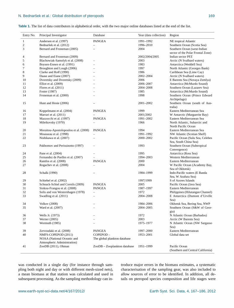
Table 1. The list of data contributors in alphabetical order, with the two major online databases listed at the end of the list.

Entry No. Principal Investigator Database Year (data collection) Region

1 Andersen et al. (1997) PANGEA 1991–1992 NE tropical Atlantic2 Bednarsek et al. (2012) – 1996–2010 Southern Ocean (Scotia Sea)3 Bernard and Froneman (2005) – 2004 Southern Ocean (west-Indian

sector of the Polar Frontal Zone)4 Bernard and Froneman (2009) 2002/2004/2005 Indian sector PFZ5 Blachowiak-Samolyk et al. (2008) – 2003 Arctic (N Svalbard waters)6 Boysen-Ennen et al. (1991) – 1983 Antarctica (Weddell Sea)7 Broughton and Lough (2006) – 1997 North Atlantic (Georges Bank)8 Clarke and Roff (1990) – 1986 Caribbean Sea (Lime Cay)9 Daase and Eiane (2007) – 2002–2004 Arctic (N Svalbard waters)10 Dvoretsky and Dvoretsky (2009) – 2006 E Barents Sea (Novaya Zemlya)11 Elliot et al. (2009) – 2006–2007 Antarctica (McMurdo Sound)12 Flores et al. (2011) – 2004–2008 Southern Ocean (Lazarev Sea)13 Foster (1987) – 1985 Antarctica (McMurdo Sound)14 Froneman et al. (2000) – 1998 Southern Ocean (Prince Edward

Archipelago)15 Hunt and Hosie (2006) – 2001–2002 Southern Ocean (south of Aus-

tralia)16 Koppelmann et al. (2004) PANGEA 1999 Eastern Mediterranean Sea17 Marrari et al. (2011) – 2001/2002 W Antarctic (Marguerite Bay)18 Mazzocchi et al. (1997) PANGEA 1991–2002 Eastern Mediterranean Sea19 Mileikovsky (1970) – 1966 North Atlantic, Subarctic and

North Pacific Ocean20 Moraitou-Apostolopoulou et al. (2008) PANGEA 1994 Eastern Mediterranean Sea21 Mousseau et al. (1998) – 1991–1992 NW Atlantic (Scotian Shelf)22 Nishikawa et al. (2007) – 2000–2002 Pacific Ocean (Sulu Sea, Celebes

Sea, South China Sea)23 Pakhomov and Perissinotto (1997) – 1993 Southern Ocean (Subtropical

Convergence)24 Pane et al. (2004) – 1995 Antarctica (Ross Sea)25 Fernandez de Puelles et al. (2007) – 1994–2003 Western Mediterranean26 Ramfos et al. (2008) PANGEA 2000 Eastern Mediterranean27 Rogachev et al. (2008) – 2004 W Pacific Ocean (Academy Bay,

Sea of Okhotsk)28 Schalk (1990) – 1984–1999 Indo-Pacific waters (E Banda

Sea, W Arafura Sea)29 Schiebel et al. (2002) 1997/1999 S of Azores Islands30 Schnack-Schiel and Cornils (2009) PANGEA 2005 Pacific Ocean (Java Sea)31 Siokou-Frangou et al. (2008) PANGEA 1987–1997 Eastern Mediterranean32 Solis and von Westernhagen (1978) – 1972 Philippines (Hilutangan Channel)33 Swadling et al. (2011) – 2004–2008 E Antarctica (Dumont d’Urville

Sea)34 Volkov (2008) – 1984–2006 Okhotsk Sea, Bering Sea, NWP35 Ward et al. (2007) – 2004–2005 Southern Ocean (S&W of Geor-

gia)36 Wells Jr. (1973) – 1972 N Atlantic Ocean (Barbados)37 Werner (2005) – 2003 Arctic (W Barents Sea)38 Wormuth (1985) – 1975–1977 N Atlantic Ocean (NW Sargasso

Sea)39 Zervoudaki et al. (2008) PANGEA 1997–2000 Eastern Mediterranean40 NMFS-COPEPOD (2011) COPEPOD – 1953–2001 Global data set

NOAA (National Oceanic and The global plankton databaseAtmospheric Administration)

41 ZooDB (2011), Ohman ZooDB – Zooplankton database 1951–1999 Pacific Ocean(Southern and Central California)

was conducted in a single day (for instance through sam-pling both night and day or with different mesh-sized nets),a mean biomass at that station was calculated and used insubsequent processing. As the sampling methodology can in-

troduce major errors in the biomass estimates, a systematiccharacterisation of the sampling gear, was also included toallow sources of error to be identified. In addition, all de-tails on pteropod species composition and life stages were

www.earth-syst-sci-data.net/4/167/2012/ Earth Syst. Sci. Data, 4, 167–186, 2012


Figure 1. The relationship between net mesh size and pteropodbiomass.

documented within the database. Where there were a num-ber of species identified per station, we also provided sum-mary statistics of total pteropod biomass per station (n=14136). The database included both Gymnosomata and The-cosomata, encompassing all genera included in the taxo-nomic tree, which was taken from Marine Species Identifi-cation Portal (http://species-identification.org) presented inFig. 3. Further subspecies levels (or formae) were not re-solved within the database. No observations of the suborderPseudothecosomata were reported in the source data sets.

2.2 Quality control

The identification and rejection of statistical outliers in thesummarised biomass data set was performed using Chau-venet’s criterion (Glover et al., 2011; Buitenhuis et al., 2012).Based on this statistical analysis, none of the stations wereexcluded as outliers (two sided z-score=4.1257).

2.3 Methodology for biomass conversion

Of the data sets obtained, the majority only reported valuesfor abundance (ind. m−3), with very few providing biomassvalues (mg m−3). Furthermore, abundance data was collectedwith varying mesh sizes and net-sampling strategies, whichmight introduce uncertainties. Therefore, we have reportedthe mesh sizes and net sampling strategy in the databasewhenever this information was available (PANGEA Table).In certain cases, multiple mesh-sized samplers were used, ofwhich we have included all descriptions available. No datawere excluded on the basis of mesh size and we examine theinfluence of mesh size in the Results section (Figs. 1 and 2).

Where direct biomass values were not available, we cal-culated biomass as a product of abundance and dry weight(DW, mg). To estimate DW, the length (L, mm) of organisms

Figure 2. Net-mesh size versus longitude (above) and latitude (be-low). Data was excluded if multiple mesh sizes were reported.

was first converted to wet weight (WW, mg) using variousconversions (see below), with subsequent conversion to dryweight (Table 2).

For many pteropod species, specific length-to-wet weightconversions were not available so more general length-weight conversions for pteropods were applied based onthose used by the GLOBal ocean ECosystems dynamics(GLOBEC) data management program. In GLOBEC, wetweights (WW) of different pteropod families were calcu-lated based on their specific body geometry and length (Lit-tle and Copley, 2003). The GLOBEC conversions coveredthe barrel shapedClionefamily of naked pteropods, the coneshaped family ofStyliola, the low-spire (globular) family ofLimacina spp., and the pyramidally shaped family ofCliospp. Accordingly, we assorted groups or species into respec-tive geometric shapes and then applied the GLOBECL toWW conversions. Although species-specific conversions arelacking for many of the groups (Table 2), we believe that thisapproach provides a reasonable first order approximation ofindividual biomass for the purpose of the present analysis.More specific details of these conversions are given below:

Equation (1) was used to convert all non-shelled (naked)taxa, including barrel-and oval- shaped families ofSpongio-branchiaspp.,PneumodermopsisandPaedoclioneand classGymnosomata (Little and Copley, 2003). Equation (2) was


http://species-identification.org


Table 2. Length to weight equations for different pteropod groups based on the geometric shapes.

SPECIES Group Equation source Conversion Equation name Equation (size-weight relationship)

Equation (Davis and Wiebe, 1985)

Limacina helicina Round/cylindrical/globular

Bednarsek et al.(2012)

Diameter→DW DW = 0.137×D1.5005

Limacinaspp. Round/cylindrical/globular

GLOBEC Diameter→DW WW =0.000194×L2.5473

WW→DW WW×0.28

Clionespp. Barell/oval-shaped (naked)

GLOBEC Length→WW Pteropod(naked: Clione)

WW =10(2.533×log(L)−3.89095)×103

WW→DW WW×0.28

Hyalocylisspp. Cone/needle/tube/bottle-shaped

GLOBEC Length→WW Pteropod (cone-shaped:Styliola)

WW = PI×L3×3/25 WW→DW WW×0.28

Styliolaspp. Cone/needle/tube/bottle-shaped


WW = PI×L3×3/25 WW→DW WW×0.28

Spongiobranchaeaspp.

Barell/oval-shaped (naked)


WW =10(2.533×log(L)−3.89095)×103

WW→DW WW×0.28

PneumodermopsisandPaedoclione

Barell/oval-shaped (naked)


WW =10(2.533×log(L)−3.89095)×103

WW→DW WW×0.28

Cavoliniaspp. Triangular/pyramidal

GLOBEC Length→DW Pteropod (Clio) WW= 0.2152×L2.293 WW→DW WW×0.28

Clio spp. Triangular/pyramidal

GLOBEC Length→WW Pteropod (Clio) WW= 0.2152×L2.293 WW→DW WW×0.28

Creseisspp. Cone/needle/tube/bottle-shaped


WW = PI×L3×3/25 WW→DW WW×0.28

Cuvierinaspp. Cone/needle/tube/bottle-shaped


WW = PI×L3×3/25 WW→DW WW×0.28

Diacria spp. Triangular/pyramidal

GLOBEC Length→WW Pteropod (Clio) WW= 0.2152×L2.293 WW→DW WW×0.28

Thecosomata Shelled Davis andWiebe (1985)

Length→WW WW = 0.2152×L2.293 WW→DW WW×0.28

Gymnosomata Naked Davis andWiebe (1985)

Length→WW WW =10(2.533×log(L)−3.89095)×103

WW→DW WW×0.28

Pteropoda Shelled Davis andWiebe (1985)

Length→WW WW = 0.2152×L2.293 WW→DW WW×0.28

applied toClione spp., being a genus species conversionequation originally derived by Boer et al. (2005):

WW = 10(2.533×log(L)−3.89095)×103, (1)

DW = 1.6146e0.0088×L. (2)

Three different shapes were distinguished within theshelled taxa, each with their ownL to WW conversions:

WW =WW = 0.2152× L2.293 triangular/pyramidal shaped

(Davis and Wiebe, 1985) (3)

WW = 0.000194× L2.5473 round/cylindrical/globular shaped

(Little and Copley, 2003) (4)

WW = PI× L3×3/25 cone/needle/bottle-shaped

(Little and Copley, 2003). (5)

Limacinidaewere one of the most abundant taxa within ourdatabase, for which there are several publishedL to DW con-versions in the literature:

DW = 0.257L2.141 (Gannefors et al., 2005) (6)

logDW= 0.685L−2.222 (Fabry, 1989) (7)

DW = 0.1365L1.501 (Bednarsek et al., 2012). (8)

Gannefors et al. (2005), Fabry (1989) and Bednarsek etal. (2012) fitted the respective functions to differing sizeranges ofLimacinidae, so we compared their performanceacross a uniform size range to consider their suitability formore broad scale application (Appendix B, Fig. B1). Thefunctional form of Fabry (1989), although optimal for ani-mals in a size range between 1 and 4 mm, became exponen-tially large at shell diameters above this range so was con-sidered unsuitable for the present analysis. The Gannefors et



949

951

953

955

957

959

961

963

965

967

969

971

973

975

977

979

981

983

984

Figure 3: Taxonomy of pteropods.985

Figure 3. Taxonomy of pteropods.

al. (2005) and Bednarsek et al. (2012) functional forms per-formed similarly well and realistically (Appendix B) acrossthe shell diameter size ranges encountered in the presentstudy (0.01 to 50 mm). We chose the Bednarsek et al. (2012)function given that its estimate of dry weight between 1 and4 mm shell diameter fell midway between the estimates ofthe Fabry (1989) and Gannefors et al. (2005) algorithms,combined with the fact that its behaviour remained realisticat larger size categories.

In cases, where the data-source referred to orders orclasses rather than species, Eq. (3) was applied since the taxawere principally non-Limacinidaeshelled species.

In the case of juveniles, the above length to weight con-versions were used according to their respective taxa or bodyshape, but the length of the veligers and larvae set at 10 % of

the adult average size, which is based on our own compar-isons of average juvenile and adult sizes.

2.3.1 Calculation of length for the individual pteropodspecies

For some data records, only the species and abundancewas recorded without any indication of individual size orweight. Individual shell diameter was therefore inferred inorder to calculate biomass. Our first step was to deter-mine size of adult specimens of each species using infor-mation from the Marine Species Identification Portal (http://species-identification.org/), of which results are presentedin Appendix C (Table C1), along with the body shape, lengthand mean size.

Where the abundance data was given for a higher taxo-nomic level than species (e.g. class, suborder, order), the av-erage length across all species within that respective taxa wasdetermined (Table C1). Because this procedure only took ac-count of adult sizes, we were aware that this would result inan overestimation of biomass. This was compensated for intwo ways: firstly, by taking into account data points where ajuvenile status was indicated (283 in total, representing 2 %of entire database) in which case length was assumed to be10 % of adult size (see above). Secondly, where the data wasnot species-specific (but family- or higher order-specific), theaverage length across all species within the taxon was cal-culated, so preventing extreme bias from very large or verysmall species.

Unfortunately, the lack of data points where both biomassand abundance values were reported made it impossible todo a quantitative comparison of the performance of ourL toW conversions.

2.3.2 Calculation of dry weight and carbon biomass fromwet weight

Wet weight was converted to dry weight using Davis andWiebe (1985):

DW =WW×0.28. (9)

Biomass was subsequently transformed to carbon using aconversion factor of 0.25, following Larson (1986).

2.3.3 Global contribution of shelled pteropods tocarbonate biomass

Once conversions from abundance to carbon biomass hadbeen completed, we considered the global biomass distribu-tion of both shelled and non-shelled pteropod taxa. Separat-ing out the shelled pteropod taxa allows the global carbonatedistribution resulting from pteropods to be assessed, so per-mitting the evaluation of their contribution to the global car-bonate budget. Bednarsek et al. (2012) have calculated inor-ganic carbon as a percentage of total organic subtracted fromtotal carbon, deducing the PIC/POC ratio of 0.27 vs. 0.73.


http://species-identification.org/



Table 3. Mean, median, maximum and minimum and standard deviation (SD) of pteropod biomass (mg C m−3) determined (i) for all globaldata, (ii) all non-zero data points, (iii) all non-zero Northern Hemisphere (NH) data-points and (iv) all non-zero Southern Hemisphere (SH)data-points.

summed biomass data mean median max min SD

all global data 4.09 0.008 5.05e+003 0.00 59.06non-zero global data 4.58 0.0145 5.05e+003 1.00e-006 62.46for the NH non-zero data 4.04 0.0145 5.05e+003 1.00e-006 64.84for the SH non-zero data 8.15 0.001 608.35 2.00e-006 45.36

986

Figure 4: Global distribution of quality-controlled pteropod data.987

Figure 4. Global distribution of quality-controlled pteropod data.

Assuming that all inorganic carbon is in the form of cal-cium carbonate, the amount of calcium carbonate can be es-timated as follows:

CaCO3 (%)= [TC (%)−TOC (%)]×8.33 (10)

where the constant 8.33 represents the molecular mass ratioof carbon to calcium carbonate.

3 Results

3.1 Global data distribution of biomass data

Altogether, we collected 25 939 data entries across alloceanic regions, which corresponded to 15 134 samples oftotal pteropod biomass (Fig. 4). Out of these, 14 136 datapoints (93 %) represented shelled pteropods (Thecosomes),and the remaining 7 % represented non-shelled pteropods(Gymnosomes). Within the whole data set, 1608 data points(11 % of all values) were reported as zero values for all ptero-pod groups.

Although pteropod observations were available for allocean basins, there was a clear bias of the data towards ob-servations in the Northern Hemisphere (NH) (77 % of non-zero entries), with the remaining 23 % in the Southern Hemi-sphere (SH, Table 3 and 6, Fig. 4). With respect to latitude,the most entries (37 %) were collected within the latitudinalband of 10–60◦ N (Table 4).

The maximum net sampling depth was 2000 m but 83 %of all nets were sampled to a maximum depth of 200 m (Ta-

ble 5). Across all observations, 62 % of all biomass occurredwithin the top 200 m, with the remaining biomass (38 %) be-ing relatively evenly distributed down to 2000 m. The deepestoccurrence of pteropods in our database was 2000 m, locatedat 81◦ N,163◦ E. The highest biomass for shelled pteropods(2980 mg C m−3) was recorded at the surface in the NH tem-perate region, at 42◦ N,70◦W. The highest biomass for thenon-shelled pteropods (5045 mg C m−3) was recorded in thesame region (42◦ N,66◦W). There were very few direct mea-surements of pteropod biomass (see Sect. 2.3), but of those,the highest recorded values were in the Sea of Okhotsk(54◦ N,138◦ E), where biomass reached 538 mg C m−3 (Ro-gachev et al., 2008).

3.2 The effect of nets and mesh sizes on global pteropodbiomass

Mesh size will influence the size range of organisms cap-tured by nets. In assembling this database, we decided toinclude all net-catch data, irrespective of mesh size. Thiswill undoubtedly create error, particularly in the undersam-pling of smaller individuals by larger meshed nets throughthe lack of retention and of larger, more motile individualsby finer meshed nets through avoidance. For the purpose ofthe present analysis, with a focus mainly on comparative pat-terns, it is important that these errors do not generate bias,since this could distort any discerned geographic trends. Weconsidered this in two ways. In Fig. 1, we compared thebiomass to net mesh size across 19 671 samples. The fig-ure shows a peak in biomass towards the mid-size meshes(∼300µm). This demonstrates that the majority of biomasslay within organisms with an equivalent spherical diameterof 300µm or greater, and that the undersampling of smallerorganisms by some studies is unlikely to have a considerableimpact on biomass estimates. Equally, the figure is indicatingthat the average biomass is similar, regardless of the meshsize used for sampling.

In Fig. 2, net mesh-size was compared to latitude. Al-though this illustrates the considerable variety of meshesused within the present database, it also shows there was noapparent bias towards certain mesh size being used at somelatitudes more than others. Therefore, although the use ofdifferent meshes between studies is undoubtedly a source of



Table 4. Latitudinal distribution of abundance data in ten degree latitudinal bands (90◦ to 90◦). Mean, maximum (max), median and standarddeviation (SD) of biomass (mg C m−3) per latitudinal band, calculated from non-zero data points.

Latitude Entries Mean SD Max Min Median(mg C m−3) (mg C m−3) (mg C m−3) (mg C m−3)

90 to 80◦ S 0 – – – – –80 to 70◦ S 72 27.20 98.44 557.41 0.001 0.1970 to 60◦ S 59 0.09 0.42 2.63 2.00e-006 060 to 50◦ S 90 13.93 35.55 168.47 0.01 0.4850 to 40◦ S 90 0.25 2.27 21.53 8.00e-006 1.32e-00440 to 30◦ S 127 0.02 0.07 0.64 2.83e-006 8.80-00530 to 20◦ S 167 0.01 0.05 0.45 5.33e-006 2.18e-00420 to 10◦ S 310 0.02 0.08 0.86 3.25e-006 6.14e-00410◦ N to 0◦ 1007 11.93 53.98 608.35 3.50e-006 00◦ to 10◦ N 1078 0.06 0.26 4.30 4.67e-006 0.0110◦ to 20◦ N 2044 1.47 8.91 226.66 1.00e-006 0.0120◦ to 30◦ N 1725 0.06 0.49 9.85 8.00e-006 0.00330◦ to 40◦ N 2958 4.51 21.65 362.89 1.00e-006 0.0140◦ to 50◦ N 744 34.76 248.13 5.05e+003 2.90e-005 0.0950◦ to 60◦ N 1960 1.26 17.26 538 0.003 0.4060◦ to 70◦ N 896 0.31 0.46 11.82 0.003 02670◦ to 80◦ N 77 17.31 61.97 517.05 1.75e-004 0.6980◦ to 90◦ N 177 4.60 10.63 34.33 1.00e-006 0.01

Table 5. Depth distribution of non-zero biomass values. Mean, maximum (max), median and standard deviation (SD) of biomass (mg C m−3)per depth interval, calculated from non-zero data points.

depth range entries Mean Max Min Median SD(m) (mg C m−3) (mg C m−3) (mg C m−3) (mg C m−3)

0–10 1806 20.65 5.45e+003 0 0.02 157.8110–25 612 14.44 557.41 0 0.04 57.5325–50 1296 3.25 434.37 0 0.002 18.2650–200 7508 0.65 308.47 0 0.02 5.74200–500 2028 0.19 9.85 0 0.002 1.04500–2000 276 0.02 3.20 0 0.004 0.18

error, it is not a major source of bias in our analyses of geo-graphic trends in pteropod biomass distribution.

3.3 Temporal distribution of data

Our database spans the period 1950–2010, and temporally,the data was fairly evenly distributed across all decades, withat least one sampling peak per decade. Several samplingpeaks were recorded in the late 1950s, then in the 1960s–1970s, followed by high numbers of data from the early1990s and 2000s. We recorded fewer samples in the 1980s(Fig. 6). To check for seasonal biases, the data was dividedinto four seasons for each hemisphere (Table 7). While in theNH, the data was distributed evenly across the four seasons(24 % in 335 spring, 23 % in summer, 24 % in autumn and30 % in winter), sampling in the SH was biased towards win-ter and summer (30 % and 25 %, respectively), with much

lower coverage during the other seasons (19 and 16 % inspring and fall, respectively).

3.4 Global biomass characteristics for all pteropodgroups and for shelled-pteropods only

For all pteropod groups combined, the range of globalbiomass concentrations was wide, spanning over four ordersof magnitude (Fig. 8a), with a mean and median biomass of4.1 mg C m−3 (SD=59.1) and 0.0083 mg C m−3 for all datapoints, and 4.6 mg C m−3 (SD=62.5) and 0.0145 mg C m−3

for non-zero biomass values, respectively. In the NH, themean biomass was 4.0 mg C m−3 (SD=64.8) and the me-dian biomass, 0.02 mg C m−3. In the SH, the mean biomasswas 8.15 mg C m−3 (SD=45.4) and the median biomass0.001 mg C m−3 (Table 3). Although the median biomass inthe SH was one order of magnitude smaller than in the NH,the mean biomass in the SH was twice that of the NH.



989

Figure 5: Number of pteropod observations as a function of latitude for the period 1950-2010.990Figure 5. Number of pteropod observations as a function of latitudefor the period 1950–2010.991

992

Figure 6: Number of observations per year, for the years 1950-2010.993Figure 6. Number of observations per year, for the years 1950–2010.

For shelled pteropod groups only, the mean and me-dian biomass for non-zero values was 3.81 mg C m−3

(SD=40.24), and 0.0078 mg C m−3, respectively, and themaximum biomass was 2979.7 mg C m−3. Considering themean biomass of shelled and non-shelled pteropods, shelledpteropods constitute 83 % to the total pteropod biomass,the remainder being made up of non-shelled pteropod taxa.When considered in terms of median biomass, 54 % wasmade up of shelled-pteropods and 46 % made up of non-shelled pteropods, indicating that the dominance of shelled-pteropods is in part due to the fact that they sometimes occurat very high concentrations.

Through assuming, firstly, an inorganic to organic car-bon ratio of 0.27 : 0.73 (Bednarsek et al., 2012) and sec-ondly an inorganic carbon to calcium carbonate molecular

Table 6. Percentage distribution of non-zero data entries with re-spect to month for the Northern (NH) and Southern (SH) Hemi-spheres.

months entries NH SH % NH % SHseason season non-zero non-zero

data data

January 1185 winter summer 8.4 11.7February 1457 winter summer 9.4 20.7March 998 spring autumn 7.4 6.1April 1298 spring autumn 9.5 9.0May 876 spring autumn 6.9 3.7June 802 summer winter 6.4 4.1July 1352 summer winter 10.4 7.1August 1790 summer winter 13.1 13.8September 1143 autumn spring 8.4 9.0October 1049 autumn spring 8.4 3.7November 859 autumn spring 6.8 3.7December 806 winter summer 5.4 10.2

mass ratio of 8.33 (Eq. 10) gave a mean global carbonatebiomass of 23.17 mg CaCO3 m−3, and a maximum biomasswas 1.81 g CaCO3 m−3. These estimates were derived fromnon-zero biomass records only.

3.4.1 Latitudinal biomass distribution

Pteropods were found at all latitudes at which samples weretaken (Figs. 5, 8a). The highest maximum, mean and me-dian biomass values were located in the NH between 40 and50◦ N (mean biomass of 5.42 mg C m−3 (SD=79.94), me-dian biomass of 0.06 mg C m−3). The highest mean and me-dian biomass values in the SH were located between 70 and80◦ S (39.71 mg C m−3 (SD=93.00) and 0.009 mg C m−3, re-spectively; Table 3). However, relatively high biomasseswere not restricted to a particular latitude or ocean basin butwere widespread, including high-latitudinal, temporal andequatorial regions in the both hemispheres. The only ex-ception was the latitudinal band between 20 and 40◦ in theNH and SH, where biomass was considerably lower (Fig. 8).There was a difference in latitudinal trends between hemi-spheres (Fig. 9a, b), with highest biomass values in the NHbeing at mid-latitudes decreasing towards the equator andthe poles, while, in the SH, highest biomass values wereseen at the poles and steadily decreasing through the mid-latitudes towards the equator. Biomass values at both poleswere within the same order of magnitude.

3.4.2 Depth distribution

Pteropods were observed at all depths down to 2000 m, al-though the funnel-shaped biomass pattern from the surfacetowards the depth indicates a sharp decrease in biomass be-low 200 m (Fig. 8b). The highest values were recorded at thesurface (0–10 m), with a mean biomass of 20.65 mg C m−3

(SD=157.81) and median biomass of 0.02 mg C m−3. Mean



Figure 7. Pteropod carbon biomass (mg C m−3) for six depth intervals:(a) surface (0–10 m),(b) 10–25 m,(c) 25–50 m,(d) 50–200 m,(e)200–500 m,(f) ≥500 m.

and median biomass gradually decrease with the depth byone order of magnitude from 10 to 200 m, and by two ordersof magnitude between the 10–200 m and 200–2000 m depthbands (Table 5, Fig. 8b).

The pattern of pteropod distribution demonstrates thathigher abundances are closely related to continental shelvesand areas of high productivity or nutrient loads (Fig. 7). Thiscan be particularly exemplified in the eastern North Pacificcentral water, which is a rather small area affected by theinflow from the more productive transitional and equatorialadjacent areas (Longhurst, 2007), with a three to four magni-tude higher biomass, in comparison to the surrounding areas.

In all ocean basins, biomass levels above 100 mg C m−3

only occurred in the 0–200 m depth layers. However, in trop-ical regions, some of the highest biomass levels were foundin the 200–500 m depth strata, where concentrations typi-cally reached between 1 and 10 mg C m−3 (Fig. 7). This sug-

gests that tropical species concentrate at deeper depths thantemperate and high-latitude species. Such geographic pat-terns in the depth distribution of pteropods have previouslybeen noted by Solis and von Westernhagen (1978), Wor-muth (1981) and Almogi-Labin et al. (1998).

3.4.3 Seasonal distribution of pteropod biomass

Seasonal variations in biomass values were much more ex-treme in the SH compared to the NH, although it is to benoted that sample coverage was comparatively greater in theNH (Table 7, Fig. 9). In both hemispheres, mean biomasspeaked in the spring. However, the peak was an order of mag-nitude higher in the SH compared to the NH (Table 7). Theratio between spring and winter biomass was approximately2 : 1 in the NH, but around 1300 : 1 in the SH. The differencein ratios is mainly explained by the virtual disappearance of



996

997

Figure 8: Above: The distribution of pteropod biomass (mg C m-3) as a function of998

latitude; (below) the relationship between pteropod biomass and net-capture depth.999

Figure 8. (Above) the distribution of pteropod biomass (mg C m−3)as a function of latitude; (below) the relationship between pteropodbiomass and net-capture depth.

pteropods in the SH during winter. Biomass levels were rel-atively similar between the NH and SH during summer andautumn. The seasonal peaks and troughs in mean biomassin both hemispheres correspond to a life-history pattern ofspring spawning, probably in response to seasonal pulses ofproductivity, as described by Hunt et al. (2008) and Bed-narsek et al. (2012).

Despite the seasonal peaks and troughs in biomass, a resid-ual biomass level was always present (Fig. 9). This indicatesthat there must be a degree of overlap in generations (Bed-narsek et al., 2012). In the higher latitudes, where there islikely just a single recruitment event per year, meaning thatthese pteropods must have a life-cycle that extends into a sec-ond year. In the Southern Ocean, Bednarsek et al. (2012) pro-posed that someLimacina helicina ant. lived for more than2 yr and, although small in number, these individuals maybe vital for future recruitment. Strong seasonality increasesthe vulnerability of early life-stages of pteropods that rely on

pulses of production to thrive (Bernard and Froneman, 2009;Seibel and Dierssen, 2003). An overlap of generations givespopulations greater stability in temporally variable environ-ments.

3.4.4 Global estimates of the pteropod biomass stockand productivity

Given representative data coverage at the both hemispheres,global mean pteropod biomass of 0.0046 g C m−3 (SD=62.5)was calculated for any point of time. To extrapolate from re-gional to global pteropod biomass, pteropod depth distribu-tion and absolute area of the global ocean are required. Withregards to depth distribution, Fig. 8a is indicative of pteropodbiomass to be uniformly distributed within the upper 300 m,and two orders of magnitude less abundant below 300 m. The300-m depth level was hence taken as a conservative esti-mate of their overall occurrence. Considering the absolutesurface area of the global deep ocean (Milliman and Drox-ler, 1996; total area equals 362.03×106 km2 cf. Dietrich etal., 1975), two values were taken to determine global ptero-pod biomass: the global ocean surface excluding shelf seas(322×106 km2) was taken as a minimum area inhibited bypteropods, while the total ocean surface area was determinedas a maximum (362.03×106 km2). Considering minimumand maximum area inhabited by pteropods, global pteropodbiomass ranges from 444 to 505 Tg of C at any point in time.This range of estimates, based on the observational resultsis similar to pteropod productivity estimate of 0.87 Pg C yr−1

obtained through modelling work by Gangstø et al. (2008).Lebrato et al. (2010) estimated global carbon productivitybudget to range between 0.96 and 2.56 Pg C yr−1. This indi-cates that pteropods contribute 20–42 % towards global car-bonate budget.

The average turnover time is known to be different for var-ious species, shorter (several months) for tropical species andlonger (more than one year) for the high-latitudinal species(Lalli and Gilmer, 1989). Here, as reported in several papers(Van der Spoel, 1973; Wells Jr., 1976; Hunt et al., 2008; etc.),the average pteropods turnover time was assumed to be oneyear, with high latitudinal species to be exceptions (e.g. Bed-narsek et al., 2012) and recorded the life cycle ofLimacinahelicina antarcticato span over 3 yr. At a global scale, and anaverage annual distribution, the entire pteropod productionwould hence amount to 444–505 Tg C yr−1, which is aboutfive times the estimated planktic foraminifers biomass pro-duction (Schiebel and Movellan, 2012: 25–100 Tg C yr−1),more than double of the estimated diazotroph biomass (Luoet al., 2012: 40–200 Tg C), and around one fifth of the to-tal diatom production (Leblanc et al., 2012: 500–3000 Tg C).Comparing global pteropod to coccolithophorid carbon pro-ductivity (Balch et al., 2007), coccolithophorid productionare approximately 1.5 to 3 times higher than our estimatedpteropod production.


178 N. Bednarsek et al.: Global distribution of pteropods1000

1001

Figure 9: Distribution of pteropod biomass values (mg C m-3) with respect to month, in the Northern Hemisphere (left) and Southern1002

Hemisphere (right).1003

1004

Figure 9. Distribution of pteropod biomass values (mg C m−3) with respect to month, in the Northern Hemisphere (left) and SouthernHemisphere (right).

Table 7. Biomass (mg C m−3) with respect to season for the Northern (NH) and Southern (SH) Hemispheres, showing the calculated mean,standard deviation (SD), median, minimum (min) and maximum (max). Biomass statistics are based on non-zero data entries only.

NH mean NH SD NH median NH min NH max SH mean SH SD SH median SH min SH max

winter 2.77 15.63 0.02 1e-006 557.41 0.03 0.09 4.54e-004 2.00e-006 1.06spring 5.42 79.94 0.06 1e-006 3.0e+003 39.71 93.00 0.009 7.50e-006 608.35summer 4.32 92.69 0.02 1e-006 5.05e+003 3.73 32.83 0.002 3.00e-006 557.41autumn 2.44 18.39 0.03 1e-006 765.24 0.51 2.47 7.28e-004 3.30e-006 21.05

4 Discussion and conclusions

The aim of this study was to collect and synthesise avail-able existing abundance and biomass data to generate thefirst global pteropod biomass database. Most studies re-ported abundance rather than biomass data, making it nec-essary to estimate carbon biomass using length to weightconversions and introducing levels of uncertainty as a result.Further uncertainties in the biomass estimates in this studywill result from sampling errors such as net-escapement andnet-avoidance, the variation in size classes between differ-ent pteropod species and generations. Further considerationsaround these uncertainties are discussed below.

With regards to the sampling error, the use of different netsfor different pteropod size classes generates uncertainty, asthe capture and filtering efficiencies differ between nets. Fur-thermore, sampling issues such as net-avoidance behaviour,extrusion of animals through mesh and clogging of the net(Harris et al., 2000) will influence abundance measurements.In addition, there is generally an insufficient use of smallermeshed nets to estimate population size. Wells Jr. (1973) pro-posed that there was a clear underestimation of the fractionof the pteropod population smaller than 100µm. As they con-stitute by far the most numerous part of the natural popula-tion (Fabry, 1989), there is a clear under-representation ofthis cohort in the scientific literature and thus of their im-portance within the microzooplankton community (Dadonand Masello, 1999). When sampling with small vertical nets,which preferentially catch small or sluggish taxa, additional

sampling errors arise from the fact that the nets can beavoided by larger plankton. On the other hand, nets withlarger mesh size can miss the mesozooplankton size fractionsincluding pteropods (Boysen-Ennen et al., 1991). We triedto address potential biases through systematic examinationof mesh sizes, net types and sampling strategies (whereveravailable in the literature) relative to biomass estimates. Ouranalyses indicated, firstly, that most biomass lay within themid-size ranges, meaning that the undersampling of smallerorganisms by some studies is unlikely to have a large impacton biomass estimates. Secondly, there was no geographicbias in the use of different nets and meshes, indicating thatsampling error is unlikely to bias analyses of geographictrends in biomass. Overall, we conclude that the documentedvariation in mesh size between studies included within thedatabase was not a source of a large-scale bias within globalbiomass patterns. Therefore, although users of the databasemust be vigilant with regards to this potential source of error,we believe that the inclusion of all data, irrespective of themesh size and sampling strategy used, maximises the poten-tial insights that can be gained from this database.

There were a number of sources of uncertainty in deriv-ing biomass values from the majority of studies within thedatabase that only provided abundance data. To convert fromabundance to biomass requires knowledge of the length dis-tribution of specimens but neither this data, nor the respectivelife-stages of specimens were commonly reported. Wheresuch information was not given, we assumed that all speci-mens were adults and used literature based estimated of body



length. This approach probably resulted in an overestimationof biomass, given that at least part of the sampled populationmay have been smaller juvenile stages. Furthermore, wheresizes were reported, there was often a lack of further statis-tical descriptors such as minimum or maximum length, sopreventing levels of variance in biomass to be estimated. Forsome species, there was no available length to weight conver-sions and so more generic algorithms were applied based onthe shape and morphological features (shelled/non-shelled)of the organisms, following the approach of GLOBEC (Lit-tle and Copley, 2003). This approach no doubt introducedfurther errors although there is little alternative to the use ofsuch generic functions until a more systematic documenta-tion of the length and weight characteristics of a wider rangeof pteropod species is undertaken.

The seasonal spread of sampling was much more even inthe NH compared to the SH. Whereas we were able to doc-ument how patterns of biomass shifted geographically be-tween seasons in the NH, our ability to achieve this was farmore constrained in the SH. In particular, sampling in winterand spring was particularly sparse in the SH. It is importantthat future sampling efforts in that hemisphere concentrateon these less sampled times of year.

This study has enabled estimates of global pteropodbiomass across a number of spatial and temporal scales. Fur-thermore, it has revealed some global patterns of pteropodbiomass, only possible due to the wealth of data availablein our data sets. Also, calculating the biomass of shelledpteropods only, we have estimated the contribution of thisgroup to the global carbonate inventory. This database hasthe potential be a valuable tool for future modelling work,both of ecosystem processes and for the study of global bio-geochemical cycles, since pteropods are a major contributorto organic and inorganic carbon fluxes. It can also make atimely contribution to the assessment of the effects of oceanacidification, particularly in terms of the vulnerability of cal-cifying species, since it provides a benchmark against whichmodel projections and future sampling efforts can be com-pared.

Appendix A

A1 Available dataset at PANGEA

A full data set containing all abundance/biomass data pointscan be downloaded from the data archive PANGAEA, Thedata file contains longitude, latitude, sampling depth (m),date (Year, Month, Day in ISO format), taxon/species/bodysize, abundance (ind. m−3), biomass (C mg m−3), meshsize (µm), sampling strategy and full data reference list(doi/journal/database)doi:10.1594/PANGAEA.777387.

A2 Gridded NetCDF biomass product

The biomass data has been gridded onto a 360×180◦ grid,with a vertical resolution of 33 WOA depth levels. Data hasbeen converted to NetCDF format for easy use in modelevaluation exercises. The NetCDF file can be downloadedfrom PANGAEA (doi:10.1594/PANGAEA.777387). It con-tains data on longitude, latitude, sampling depth (m), month,abundance (ind. m−3) and biomass (mg C m−3).

2005

(2012)

Figure B1. Shell diameter to dry weight relationships forLimacinahelicinaderived by three different studies.





Table C1. Body dimensions and shapes of a range of shelled and non-shelled pteropod species (source: Marine identification portal (http://species-identification.org/), except forClione limacina∗ – Boer et al., 2005).

Order Suborder Taxon Subspecies/Formae

Mean shelllength (mm)

Mean shellwidth (mm)

Body length(mm)

Shell/bodyshape

Additionalinformation

Group

Thecosomata EuthecosomataLimacina helicina helicinahelicina

6 8 round left coiled shell,moderately highlyspired, aperturehigher than wide,height/diameter ra-tion=0.75

Round/cylindrical/globular

Thecosomata EuthecosomataLimacina helicina helicinapacifica

5 2 Round/cylindrical/globular

Thecosomata EuthecosomataLimacinaretroversa

retroversa 2.5 2.6 round small, left coiledshell, no umbilicalkeel, spire moder-ately highly coiled


Thecosomata EuthecosomataLimacinabulimoides

2 1.4 round highly coiled spire Round/cylindrical/globular

Thecosomata EuthecosomataLimacina inflata 1.3 round coiled nearly in onelevel; average shelldiameter=0.86,aperturelength=0.68 mm,diameter of oper-culum=0.31 mm,aperturebreadth=0.5 mm


Thecosomata EuthecosomataLimacina helicina antarctica 5 round left coiled, spirevariable


Thecosomata EuthecosomataLimacina helicina antarcticaantarcticarangii

2 3.5 Round/cylindrical/globular

Thecosomata EuthecosomataLimacinatrochiformis

1 0.8 round left coiled, apicalangle 75–96◦


Thecosomata EuthecosomataLimacina helicinaspp.average

4.22 Round/cylindrical/globular

Thecosomata EuthecosomataLimacinatrochiformis

1 0.8 round left coiled, apicalangle 75–96◦


Thecosomata EuthecosomataLimacina lesueuri 0.8 1 round flatly left coiled,spire depressed;max diameterof operculum= 0.6 mm andlength/widthratio=2/3


Thecosomata EuthecosomataLimacinaspp. 2.98 the length calcu-lated as the averageof all species


Gymnosomata Clione limacina limacinaantarctica

25 Up to 40 barrel body pointed pos-teriorly

Barrel/oval-shaped (naked)

Gymnosomata Clione limacina limacinameridionalis

21 20 barrel Cone elongated Barrel/oval-shaped (naked)

Gymnosomata Clione limacina∗ 12 Barrel/oval-shaped (naked)

Gymnosomata Clione limacinalarvae

0.3

Gymnosomata Clionespp. 14.57 the length calcu-lated as the averageof all species


Thecosomata EuthecosomataHyalocylis striata 8 up to 8 cylindrical uncoiled, cross-section round,shell curved faintlydorsally; rear angleof adult shell 24◦

Cone-shaped(needle/tube/bottle)





Table C1. Continued.




Body length(mm)

Shell/bodyshape


Group

Thecosomata EuthecosomataStyliola subula 13 13 needle-like shell is (conical),uncoiled, the cross-section is round,long, tubular, notcurved; rear angleof shell is 11◦

Cone-shaped(needle/tube/bottle)

Gymnosomata Spongiobranchaeaaustralis

20 max 22 oval long body Barrel/oval-shaped (naked)

Gymnosomata Spongiobrachaeaaustralis juv.

10 Barrel/oval-shaped (naked)

Gymnosomata Spongiobranchaeaspp.

15 Barrel/oval-shaped (naked)

Gymnosomata Pneumodermopsis teschi up to 9.1 barrel Barrel/oval-shaped (naked)

Gymnosomata Pneumodermopsis pulex up to 8 barrel Barrel/oval-shaped (naked)

Gymnosomata Pneumodermopsis macrochira up to 2 barrel Barrel/oval-shaped (naked)

Gymnosomata Pneumodermopsis ciliata up to 15 barrel slender body Barrel/oval-shaped (naked)

Gymnosomata Pneumodermopsis spoeli up to 3 (2.6) barrel body rounded thencontracted


Gymnosomata Pneumodermopsis simplex up to 5 (4.5) barrel Barrel/oval-shaped (naked)

Gymnosomata Pneumodermopsis paucidens up to 5 barrel Barrel/oval-shaped (naked)

Gymnosomata Pneumodermopsis canephora up to 12 barrel Barrel/oval-shaped (naked)

Gymnosomata Pneumodermopsis polycotyla up to 5 barrel Barrel/oval-shaped (naked)

Gymnosomata Pneumodermopsisspp.

6.5 the length calcu-lated as the averageof all species


Gymnosomata Paedocline doliiformis 1.5 elongate oval tocylindrical shape

Barrel/oval-shaped (naked

Thecosomata EuthecosomataCavoliniaglobulosa

6 4.5 globular Triangular/pyra-midal

Thecosomata EuthecosomataCavolinia inflexa inflexa 7 5 6 triangular Triangular/pyra-midal

Thecosomata EuthecosomataCavolinia inflexa imitans 8 triangular Triangular/pyra-midal

Thecosomata EuthecosomataCavolinia inflexa labiata 8 5.5 triangular Triangular/pyra-midal

Thecosomata EuthecosomataCavolinialongirostris

f. longirostris 6.2 6.8–4.9 7 triangular accepted nameDicavolinialongirostris

Triangular/pyra-midal


f. angulosa 3.9 3.7–2.3 5 triangular accepted nameDicavolinialongirostris



f. strangulata 4 4.1–2.7 5 triangular accepted nameDicavolinialongirostris


Thecosomata EuthecosomataCavolinia uncinata uncinata unci-nata

6.5 4.0–6.6 8 triangular uncoiled shell Triangular/pyra-midal

Thecosomata EuthecosomataCavolinia uncinata uncinata f. pul-satapusilla

6.1 9.5 triangular Triangular/pyra-midal

Thecosomata EuthecosomataCavoliniaspp. 6.2 the length calcu-lated as the averageof all species


Thecosomata EuthecosomataClio convexa 8 4.5 up to 8 pyramidal shell uncoiled Triangular/pyra-midal







Body length(mm)

Shell/bodyshape


Group

Thecosomata EuthecosomataClio cuspidata 20 30 up to 20 pyramidal shell uncoiled Triangular/pyra-midal

Thecosomata EuthecosomataClio piatkowskii 13.5 16 14 broad pyra-midal


Thecosomata EuthecosomataClio pyramidata 20 10 pyramidal Triangular/pyra-midal

Thecosomata EuthecosomataClio pyramidata martensi 17 Triangular/pyra-midal

Thecosomata EuthecosomataClio pyramidata antarctica 17 Triangular/pyra-midal

Thecosomata EuthecosomataClio pyramidata lanceolata 20 Triangular/pyra-midal

Thecosomata EuthecosomataClio pyramidataspp.

18.5 Triangular/pyra-midal

Thecosomata EuthecosomataClio spp. 16.5 the length calcu-lated as the averageof all species


Thecosomata EuthecosomataCreseis acicula acicula 33 1.5 tube shell is not curved,cross-section circu-lar, extremely longand narrow, aper-ture rounded, rearangle of shell 13–14◦

Cone-shaped(+needle/tube/bottle)

Thecosomata EuthecosomataCreseis acicula clava 6 Cone-shaped(+needle/tube/bottle)

Thecosomata EuthecosomataCreseis aciculaspp.

19.5 Cone-shaped(+needle/tube/bottle)

Thecosomata EuthecosomataCreseis virgula virgula 6 max 2 6 tube shell is curved(distinctly curveddorsally), uncoiled,long and narrow


Thecosomata EuthecosomataCreseis virgula conica 7 aperture-diameter=1 mm

up to 7 tube shell curved andslender, cross-section is round


Thecosomata EuthecosomataCreseis virgula constricta 3.5 0.4 4 tube uncoiled shell,cross-sectionround, short andnarrow, slightlycurved


Thecosomata EuthecosomataCreseis virgulaspp.

5.5 0.2 tube Cone-shaped(+needle/tube/bottle)

Thecosomata EuthecosomataCreseisspp. 11.5 the length calcu-lated as the averageof all species


Thecosomata EuthecosomataCuvierinacolumnella

columnella 10 3 up to 10 bottle-shaped

the greatest shellwidth is found atless than 173 of theshell length fromposterior


Thecosomata EuthecosomataDiacria costata 2.3 1.7–2.2 3 globular shell uncoiled Triangular/pyra-midal

Thecosomata EuthecosomataDiacria danae 1.7 1.1–1.7 2 globular shell uncoiled Triangular/pyra-midal

Thecosomata EuthecosomataDiacria quadriden-tata

3 1.8–2.5 2 globular shell uncoiled Triangular/pyra-midal







Body length(mm)

Shell/bodyshape


Group

Thecosomata EuthecosomataDiacria rampali 9.5 9 9 cone-shaped bilateral symmetri-cal, uncoiled shell,slender, longcaudal spine;spine markwidth=0.95 mm,apertureheight=0.95.


Thecosomata EuthecosomataDiacria trispinosa trispinosa 8 10 1 cone-shaped bilateral symmetri-cal, uncoiled shell,long caudal spine;the ration upperlip-spine tip/spinetip-membrane=1.3,spine markwidth=1.5 mm,apertureheight=0.9 mm.


Thecosomata EuthecosomataDiacria major 10.7 11 uncoiled bilateralsymmetrical, longcaudal spine; ratioupperlip-spinetip/spine-tip mem-brane=1,.65 mm,spine markwidth=1.2 mm,apertureheight=1 mm;


Thecosomata EuthecosomataDiacria spp. 5.9 the length calcu-lated as the averageof all species


THECOSOMATACOMBINED

8.1 shelled

GYMNOSOMATACOMBINED

12.0 naked

PTEROPODACOMBINED

8.9 shelled

Acknowledgements. We thank K. Blachowiak-Samolyk,E. Boysen-Ennen, E. A. Broughton, C. Clarke, M. Daase,V. G. Dvoretsky, T. D. Elliot, H. Flores, B. A. Foster, P. W. Frone-man, B. P. V. Hunt, L. Mousseau, J. Nishikawa, M. D. Ohman,T. O’Brien, E. A. Pakhomov, L. Pane, M. Fernandez de Puelles,K. A. Rogachev, P. H. Schalk, N. Solis, K. M. Swadling,A. F. Volkov, P. Ward, I. Werner, J. H. Wormuth for a permission touse and republish their data on pteropods in the MAREDAT projectand this paper.

The lead author is grateful to R. A. Feely (NOAA) and R. Schiebel(Universite d’Angers-BIAF) for their invaluable advice and ideas.Thanks also go to Marko Vuckovic from the University of NovaGorica for the help with the Matlab software changes. The work atETH for NB was partly funded through an Erasmus scholarship.GT was supported by the Ecosystems core research programme atthe British Antarcttic Survey. The research leading to these resultshas received funding from the European Community’s SeventhFramework Programme (FP7 2007–2013) under grant agreementno. 238366.

Edited by: W. Smith

References

Almogi-Labin, A., Hemleben, C., and Meischner, D.: Carbonatepreservation and climatic changes in the central Red Sea duringthe last 380 kyr as recorded by pteropods, Marine Micropaleon-tology, 33, 87–107,doi:10.1016/S0377-8398(97)00034-0, 1998.

Acker, J. G. and Byrne, R. H.: The influence of surface state andsaturation state on the dissolution kinetics of biogenic aragonitein seawater, Am. J. Sci., 289, 1098–1116, 1989.

Andersen, V., Sardou, J., and Gasser, B.: Macroplankton and mi-cronekton in the northeast tropical Atlantic: abundance, com-munity composition and vertical distribution in relation to dif-ferent trophic environments, Deep-Sea Res. Pt. I, 44, 193–222,doi:10.1016/S0967-0637(96)00109-4, 1997.

Bednarsek, N., Tarling, G., Fielding, S., and Bakker, D.: Populationdynamics and biogeochemical significance ofLimacina helic-ina antarticain the Scotia Sea (Southern Ocean), Deep-Sea Res.Pt. II, 59–60, 105–116,doi:10.1016/j.dsr2.2011.08.003, 2012.


http://dx.doi.org/10.1016/S0377-8398(97)00034-0

http://dx.doi.org/10.1016/S0967-0637(96)00109-4

http://dx.doi.org/10.1016/j.dsr2.2011.08.003


Bernard, K. S. and Froneman, P. W.: Trophodynamics of se-lected mesozooplankton in the west-Indian sector of the Po-lar Frontal Zone, Southern Ocean, Polar Biol., 28, 594–606,doi:10.1007/s00300-005-0728-3, 2005.

Bernard, K. S. and Froneman, P. W.: The sub-Antarctic eu-thecosome pteropod,Limacina retroversa: Distribution pat-terns and trophic role, Deep-Sea Res. Pt. I, 56, 582–598,doi:10.1016/j.dsr.2008.11.007, 2009.

Berner, R. A. and Honjo, S.: Pelagic sedimentation of aragonite: itsgeochemical significance, Science, 211, 940–942, 1981.

Blachowiak-Samolyk, K., Søreide, J. E., Kwasniewski, S., Sund-fjord, A., Hop, H., Falk-Petersen, S., and Hegseth, E. N.: Hydro-dynamic control of mesozooplankton abundance and biomass innorthern Svalbard waters (79–81◦ N), Deep-Sea Res. Pt. II, 55,2210–2224, 2008.

Boer, M., Gannefors, C., Kattner, G., Graeve, M., Hop, H., and Falk-Petersen, S.: The Arctic pteropodClione limacina: seasonal lipiddynamics and life-strategy, Mar. Biol., 147, 707–717, 2005.

Boysen-Ennen, E., Hagen, W., Hubold, G., and Piatkowski, U.:Zooplankton biomass in the ice-covered Weddell Sea, Antarc-tica, Mar. Biol., 111, 227–235, 1991.

Broughton, E. A. and Lough, R. G.: A direct comparison ofMOCNESS and Video Plankton Recorder zooplankton abun-dance estimates: Possible application for augmenting net sam-pling with video systems, Deep-Sea Res. Pt. II, 53, 2789–2807,doi:10.1016/j.dsr2.2006.08.013, 2006.

Buitenhuis, E. T., Vogt, M., Moriarty, R., Bednarsek, N., Doney, S.C., Leblanc, K., Le Quere, C., Luo, Y.-W., O’Brien, C., O’Brien,T., Peloquin, J., Schiebel, R., and Swan, C.: MAREDAT: to-wards a World Ocean Atlas of MARine Ecosystem DATa, EarthSyst. Sci. Data Discuss., 5, 1077–1106,doi:10.5194/essdd-5-1077-2012, 2012.

Clarke, C. and Roff, J. C.: Abundance and Biomass of HerbivorousZooplankton off Kingston, Jamaica, with Estimates of their An-nual Production, Estuar. Coast. Shelf S., 31, 423–437, 1990.

Daase, M. and Eiane, K.: Mesozooplankton distribution in northernSvalbard waters in relation to hydrography, Polar Biol., 30, 969–981,doi:10.1007/s00300-007-0255-5, 2007.

Dadon, J. R. and Masello, J. F.: Mechanisms generating and main-taining the admixture of zooplanktonic molluscs (Euthecoso-mata: Opistobranchiata: Gastropoda) in the Subtropical Front ofthe South Atlantic, Mar. Biol., 135, 171–179, 1999.

Davis, C. S. and Wiebe, P. H.: Macrozooplankton Biomass in aWarm-Core Gulf Stream Ring: Time Series Changes in SizeStructure, Taxonomic Composition, and Vertical Distribution, J.Geophys. Res., 90, 8871–8884, 1985.

Dietrich, G., Kalle, K., Krauss, W., and Siedler, G.: AllgemeineMeereskunde, 3, Auflage, Gebruder Borntrager, Berlin, Stuttgart,593 pp., 1975.

Dvoretsky, V. G. and Dvoretsky, A. G.: Summer mesozooplank-ton distribution near Novaya Zemlya (eastern Barents Sea), PolarBiol., 32, 719–731,doi:10.1007/s00300-008-0576-z, 2009.

Elliot, T. D., Tang, K. W., and Shields, A. R.: Mesozooplankton be-neath the summer sea ice in McMurdo Sound, Antarctica: abun-dance, species composition and DMSP content, Polar Biol., 32,113–122,doi:10.1007/s00300-008-0511-3, 2009.

Fabry, V. J.: Aragonite production by pteropod molluscs in the sub-arctic Pacific, Deep-Sea Res., 36, 1735–1751,doi:10.1016/0198-0149(89)90069-1, 1989.

Fernandez de Puelles, M. L., Alemany, F., and Jansa, J.: Zooplank-ton time-series in the Balearic Sea (Western Mediterranean):Variability during the decade 1994–2003, Prog. Oceanogr., 74,329–354,doi:10.1016/j.pocean.2007.04.009, 2007.

Flores, H., van Franeker, J.-A., Cisewski, B., Leach, H., van dePutte, A. P., Meesters, E. H. W. G., Bathmann, U., and Wolff,W. J.: Macrofauna under sea ice and in the open surface layerof the Lazarev Sea, Southern Ocean, Deep-Sea Res. Pt. II, 58,1948–1961,doi:10.1016/j.dsr2.2011.01.010, 2011.

Foster, B. A.: Composition and Abundance of Zooplankton Underthe Spring Sea Ice of McMurdo Sound, Antarctica, Polar Biol.,8, 41–48, 1987.

Froneman, P. W., Pakhomov, E. A., and Treasure, A.: Trophic im-portance of the hyperiid amphipod,Themisto gaudichaudi, in thePrince Edward Archipelago (Southern Ocean), Polar Biol., 23,429–436, 2000.

Gannefors, C., Boer, M., Kattner, G., Graeve, M., Eiane, K., Gullik-sen, B., Hop, H., and Falk-Petersen, S.: The Arctic sea butterflyLimacina helicina: lipids and life strategy, Mar. Biol., 147, 169–177,doi:10.1007/s00227-004-1544-y, 2005.

Gangstø, R., Gehlen, M., Schneider, B., Bopp, L., Aumont, O., andJoos, F.: Modeling the marine aragonite cycle: changes under ris-ing carbon dioxide and its role in shallow water CaCO3 disso-lution, Biogeosciences, 5, 1057–1072,doi:10.5194/bg-5-1057-2008, 2008.

Gilmer, R. W.: In situ observations of feeding in thecosomatouspteropod molluscs, Am. Malacol. Bull., 8, 53–59, 1990.

Gilmer, R. W. and Harbison, G. R.: Diet ofLimacina helicina(Gas-tropoda: Thecosomata) in Arctic waters in midsummer, Mar.Ecol.-Prog. Ser., 77, 125–134, 1991.

Glover, D. M., Jenkinds, W. J., and Doney, S. C.: ModellingMethods for Marine Science, Cambridge University Press, Cam-bridge, UK, ISBN 978-0-521-86783-2, 2011.

Harbison, G. R. and Gilmer, R. W.: Swimming, buoyancyand feeding in shelled pteropods: a comparison of fieldand laboratory observations, J. Mollus. Stud., 58, 337–339,doi:10.1093/mollus/58.3.337, 1992.

Harris, R. P., Wiebe, P. H., Lenz, J., Skjoldal, H.-R., and Hunt-ley, M.: Zooplankton methodology manual, Elsevier AcademicPress, London, UK, 684 pp., 2000.

Hopkins, T. L.: Midwater food web in McMurdo Sound, Ross Sea,Antarctica, Mar. Biol., 96, 93–106,doi:10.1007/BF00394842,1987.

Hunt, B. P. V. and Hosie, G. H.: The seasonal succession ofzooplankton in the Southern Ocean south of Australia, part I:The seasonal ice zone, Deep-Sea Res. Pt. I, 53, 1182–1202,doi:10.1016/j.dsr.2006.05.001, 2006.

Hunt, B. P. V., Pakhomov, E. A., Hosie, G. W., Siegel, V., Ward, P.,and Bernard, K.: Pteropods in Southern Ocean ecosystems, Prog.Oceanogr., 78, 193–221,doi:10.1016/j.pocean.2008.06.001,2008.

Jackson, G. A., Najjar, R. G., and Toggweiler, J. R.: Flux feed-ing as a mechanism for zooplankton grazing and its implicationsfor vertical particulate flux, Limnol. Oceanogr., 38, 1328–1332,1993.

Karnovsky, N. J., Hobson, K. A., Iverson, S., and Hunt Jr., G. L.:Seasonal changes in the diets of seabirds in the North WaterPolynya: a multiple-indicator approach, Mar. Ecol.-Prog. Ser.,357, 291–299, 2008.


http://dx.doi.org/10.1007/s00300-005-0728-3

http://dx.doi.org/10.1016/j.dsr.2008.11.007


http://dx.doi.org/10.5194/essdd-5-1077-2012


http://dx.doi.org/10.1007/s00300-007-0255-5

http://dx.doi.org/10.1007/s00300-008-0576-z

http://dx.doi.org/10.1007/s00300-008-0511-3

http://dx.doi.org/10.1016/0198-0149(89)90069-1

http://dx.doi.org/10.1016/0198-0149(89)90069-1

http://dx.doi.org/10.1016/j.pocean.2007.04.009


http://dx.doi.org/10.1007/s00227-004-1544-y

http://dx.doi.org/10.5194/bg-5-1057-2008

http://dx.doi.org/10.5194/bg-5-1057-2008

http://dx.doi.org/10.1093/mollus/58.3.337

http://dx.doi.org/10.1007/BF00394842


http://dx.doi.org/10.1016/j.pocean.2008.06.001


Koppelmann, R., Weikert, H., Halsband-Lenk, C., and Jennerjahn,T. C.: Mesozooplankton community respiration and its relationto particle flux in the oligotrophic eastern Mediterranean, GlobalBiogeochem. Cy., 18, GB1039,doi:10.1029/2003GB002121,2004.

Lalli, C. M.: Structure and function of the buccal apparatus ofClione limacina(Phipps) with a review of feeding in gymnoso-matous pteropods, J. Exp. Mar. Biol. Ass. UK, 4, 101–118, 1970.

Lalli, C. M. and Gilmer, R. W.: Pelagic snails: the biology ofholoplanktonic gastropod molluscs, Stanford, Stanford Univer-sity Press, California, 1989.

Larson, R. J.: Water content, organic content, and carbon andnitrogen composition of medusae from the northeast Pacific,J. Exp. Mar. Biol. Ecol., 99, 107–120,doi:10.1016/0022-0981(86)90231-5, 1986.

Leblanc, K., Aristegui, J., Armand, L., Assmy, P., Beker, B., Bode,A., Breton, E., Cornet, V., Gibson, J., Gosselin, M.-P., Kopczyn-ska, E., Marshall, H., Peloquin, J., Piontkovski, S., Poulton,A. J., Queguiner, B., Schiebel, R., Shipe, R., Stefels, J., vanLeeuwe, M. A., Varela, M., Widdicombe, C., and Yallop, M.:A global diatom database – abundance, biovolume and biomassin the world ocean, Earth Syst. Sci. Data Discuss., 5, 147–185,doi:10.5194/essdd-5-147-2012, 2012.

Le Quere, C., Harrison, S. P., Prentice, C., Buitenhuis, E. T., Au-monts, O., Bopp, L., Claustre, H., da Cunha, L. C., Geider, R.,Giraud, X., Klaas, C., Kohfeld, K. E., Legendre, L., Manizza, M.,Plattss, T., Rivkin, R., Sathyendranath, S., Uitz, J., Watson, A. J.,Wolf-Gladrow, D.: Ecosystem dynamics based on plankton func-tional types for global ocean biochemistry models, Glob. ChangeBiol., 11, 2016–2040, 2005.

Little, W. S. and Copley, N. J.: WHOI Silhouette DIGITIZER, Ver-sion 1.0, Users Guide, WHOI Technical Report, Woods HoleOceanographic Institution, 2003.

Lochte, K. and Pfannkuche, O.: Processes driven by the small sizedorganisms at the water-sediment interface, in: Ocean Margin Sys-tems, edited by: Wefer, G., Billet, D., Hebbeln, D., Jørgensen, B.B., Schluter, M., and Weering, T. C., Springer, Heidelberg, Ger-many, 2003.

Longhurst, A.: Ecological Geography of the Sea, Academic Press,USA, 2007.

Luo, Y.-W., Doney, S. C., Anderson, L. A., Benavides, M., Bode,A., Bonnet, S., Bostrom, K. H., Bottjer, D., Capone, D. G., Car-penter, E. J., Chen, Y. L., Church, M. J., Dore, J. E., Falcon, L.I., Fernandez, A., Foster, R. A., Furuya, K., Gomez, F., Gunder-sen, K., Hynes, A. M., Karl, D. M., Kitajima, S., Langlois, R.J., LaRoche, J., Letelier, R. M., Maranon, E., McGillicuddy Jr.,D. J., Moisander, P. H., Moore, C. M., Mourino-Carballido, B.,Mulholland, M. R., Needoba, J. A., Orcutt, K. M., Poulton, A.J., Raimbault, P., Rees, A. P., Riemann, L., Shiozaki, T., Sub-ramaniam, A., Tyrrell, T., Turk-Kubo, K. A., Varela, M., Vil-lareal, T. A., Webb, E. A., White, A. E., Wu, J., and Zehr, J. P.:Database of diazotrophs in global ocean: abundances, biomassand nitrogen fixation rates, Earth Syst. Sci. Data Discuss., 5, 47–106,doi:10.5194/essdd-5-47-2012, 2012.

Marrari, M., Daly, K. L., Timonin, A., and Semenova, T.: The zoo-plankton of Marguerite Bay, Western Antarctic Peninsula – PartI: Abundance, distribution, and population response to variabil-ity in environmental conditions, Deep-Sea Res. Pt. II, 58, 1599–1613,doi:10.1016/j.dsr2.2010.12.007, 2011.

Mazzocchi, M. G., Christou, E., Rastaman, N., and Siokou-Frangou, I.: Mesozooplankton distribution from Sicily to Cyprus(Eastern Mediterranean): I. General aspects, Oceanol. Acta, 20,521–535, 1997.

Mileikovsky, S. A.: Breeding and larval distribution of the ptero-podClione limacinain the North Atlantic, Subarctic and NorthPacific Oceans, Mar. Biol., 6, 317–334, 1970.

Milliman, J. D. and Droxler, A. W.: Neritic and pelagic carbonatesedimentation in the marine environment: Ignorance is not bliss,Geologische Rundschau, 85, 496–504, 1996.

Moraitou-Apostolopoulou, M., Zervoudaki, S., and Kapiris, K.:Mesozooplankton abundance in waters of the Aegean Sea, Hel-lenic Center of Marine Research, Institut of Oceanography, Hy-drodynamics and Biogeochemical Fluxes in the Straits of theCretan Arc (project), Greece, 2008.

Mousseau, L., Fortier, L., and Legendre, L.: Annual production offish larvae and their prey in relation to size-fractioned primaryproduction (Scotian Shelf, NW Atlantic), ICES J. Mar. Sci., 55,44–57, 1998.

Nishikawa, J., Matsuura, H., Castillo, L. V., Wilfredo, L. C.,and Nishida, S.: Biomass, vertical distribution and com-munity structure of mesozooplankton in the Sulu Sea andits adjacent waters, Deep-Sea Res. Pt. II, 54, 114–130,doi:10.1016/j.dsr2.2006.09.005, 2007.

NMFS-COPEPOD: The Global Plankton Database, NOAA Na-tional Oceanic and Atmospheric Administration, US Departmentof Commerce (http://www.st.nfms.noaa.gov/plankton), 2011.

Pakhomov, E. A. and Perissinotto, R.: Mesozooplankton commu-nity structure and grazing impact in the region of the Subtropi-cal Convergence south of Africa, J. Plankton Res., 19, 675–691,1997.

Pane, L., Feletti, M., Francomacaro, B., and Mariottini, G.L.: Summer coastal zooplankton biomass and copepod com-munity structure near Italian Terra Nova Base (Terra NovaBay, Ross Sea, Antarctica), J. Plankton Res., 26, 1479–1488,doi:10.1093/plankt/fbh135, 2004.

Perissinotto, R.: Mesozooplankton size-selectivity and grazing im-pact on the phytoplankton community of the Prince EdwardArchipelago (Southern Ocean), Mar. Ecol.-Prog. Ser., 79, 243–258, 1992.

Ramfos, A., Isari, S., and Rastaman, N.: Mesozooplankton abun-dance in water of the Ionian Sea (March 2000), Department ofBiology, University of Patras, 2008.

Rogachev, K. A., Carmack, E. C., and Foreman, M. G. G.: Bowheadwhales feed on plankton concentrated by estuarine and tidal cur-rents in Academy Bay, Sea of Okhotsk, Cont. Shelf Res., 28,1811–1826,doi:10.1016/j.csr.2008.04.014, 2008.

Schalk, P. H.: Spatial and seasonal variation in pteropods (Mol-lusca) of Indo-Malayan waters related to watermass distribution,Mar. Biol., 105, 59–71, 1990.

Schiebel, R. and Movellan, A.: First-order estimate of the plankticforaminifer biomass in the modern ocean, Earth Syst. Sci. Data,4, 75–89,doi:10.5194/essd-4-75-2012, 2012.

Schiebel, R., Waniek, J., Zeltner, A., and Alves, M.: Impact ofthe Azores Front on the distribution of planktic foraminifers,shelled gastropods, and coccolithophorids, Deep-Sea Res. Pt. II,49, 4035–4050, 2002.

Schnack-Schiel, S. B. and Cornils, A.: Zooplankton abundancemeasured on Apstein net samples during cruise CISKA2005,


http://dx.doi.org/10.1029/2003GB002121

http://dx.doi.org/10.1016/0022-0981(86)90231-5

http://dx.doi.org/10.1016/0022-0981(86)90231-5





http://www.st.nfms.noaa.gov/plankton

http://dx.doi.org/10.1093/plankt/fbh135

http://dx.doi.org/10.1016/j.csr.2008.04.014

http://dx.doi.org/10.5194/essd-4-75-2012


Alfred Wegener Institute for Polar and Marine Research, Sciencefor the Protection of Indonesian Coastal Environment (project),Bremerhaven, 2009.

Seibel, B. A. and Dierssen, H. M.: Cascading trophic impacts ofreduced biomass in the Ross Sea, Antarctica: Just the tip of theiceberg?, Biol. Bull., 205, 93–97, 2003.

Siokou-Frangou, I., Christou, E., and Rastman, N.: Mesozooplank-ton abundance in waters of the Ionian Sea, Hellenic Center ofMarine Research, Institut of Oceanography, Physical Oceanog-raphy of the Eastern Mediterranean (project), Greece, 2008.

Solis, N. B. and von Westernhagen, H.: Vertical distribution of Eu-thecosomatous Pteropods in the Upper 100 m of the HilutanganChannel, Cebu, The Philippines, Mar. Biol., 48, 79–87, 1978.

Swadling, K. M., Penot, F., Vallet, C., Rouyer, A., Gasparini, S.,Mousseau, L., Smith, M., and Goffart, A.: Interannual vari-ability of zooplankton in the Dumont d’Urville sea (139◦ E–146◦ E), east Antarctica, 2004–2008, Polar Sci., 5, 118–133,doi:10.1016/j.polar.2011.03.001, 2011.

Treguer, P., Legendre, L., Rivkin, R. T., Raueneau, O., and Dit-tert, N.: Water column biogeochemistry below the euphotic zone,Ocean biogeochemistry: The role of the ocean carbon cycle inglobal change, edited by: Fasham, M. J. R., Global Change – TheIGBP Series (closed), 145–156,doi:10.1007/978-3-642-55844-3 7, 2003.

Van der Spoel, S.: Growth, reproduction and vertical migration inClio pyramidataLinne, 1767 formalunceolata(Lesueur, 1813),with notes on some other Cavoliniidae (Mollusca, Pteropoda),Beaufortia, 281, 117–134, 1973.

Volkov, A. F.: Mean Annual Characteristics of Zooplanktonin the Sea of Okhotsk, Bering Sea and Northwestern Pa-cific (Annual and Seasonal Biomass Values and Predomi-nance, ISSN 1063-0740, Russ. J. Mar. Biol., 34, 437–415,doi:10.1134/S106307400807002X, 2008.

Ward, P., Whitehouse, M., Shreeve, R., Thorpe, S., Atkinson, A.,Korb, R., Pond, D., and Young, E.: Plankton community structuresouth and west of South Georgia (Southern Ocean): Links withproduction and physical forcing, Deep-Sea Res. Pt. I, 54, 1871–1889,doi:10.1016/j.dsr.2007.08.008, 2007.

Wells Jr., F. E.: Effects of Mesh Size on Estimation of PopulationDensities of Tropical Euthecosomateus Pteropods, Mar. Biol.,20, 347–350, 1973.

Wells Jr., F. E.: Seasonal patterns of abundance and reproduction ofeuthecosomatous pteropods off Barbados, West Indies, Veliger,18, 241–248, 1976.

Werner, I.: Living conditions, abundance and biomass of under-icefauna in the Storfjord area (Western Barents Sea, Arctic) in latewinter (March 2003), Polar Biol., 28, 311–318, 2005.

Wormuth, J. H.: Vertical distributions and diel migrations of Eu-thecosomata in the northwest Sargasso Sea, Deep-Sea Res., 28,1493–1515,doi:10.1016/0198-0149(81)90094-7, 1981.

Wormuth, J. H.: The role of cold-core Gulf Stream rings in the tem-poral and spatial patterns of euthecosomatous pteropods, Deep-Sea Res., 32, 773–788, 1985.

Zervoudaki, S., Christou, E., Siokou-Frangou, I., and Zoulias, T.:Mesozooplankton abundance in water of the Aegean Sea, Hel-lenic Center of Marine Research, Institut of Oceanography, In-vest. of new marine biol. resources in deep waters of Ionian andAegean Seas, Greece, 2008.

ZooDB – Zooplankton database, Plankton sample analysis sup-ported by NSF grants to M. D. Ohman, Scripps Institution ofOceanography and by the SIO Pelagic Invertebrates Collection,http://oceaninformatics.ucsd.edu/zoodb/#, 2011.


http://dx.doi.org/10.1016/j.polar.2011.03.001

http://dx.doi.org/10.1007/978-3-642-55844-3_7

http://dx.doi.org/10.1007/978-3-642-55844-3_7

http://dx.doi.org/10.1134/S106307400807002X


http://dx.doi.org/10.1016/0198-0149(81)90094-7

http://oceaninformatics.ucsd.edu/zoodb/#

Documents

Social - ESSD...10 Dvoretsky and Dvoretsky (2009) – 2006 E Barents Sea (Novaya Zemlya) 11 Elliot et al. (2009) – 2006–2007 Antarctica (McMurdo Sound) 12 Flores et al. (2011)