Social Identity, Electoral Institutions, and the Number ofCandidates

Eric S. DicksonNew York University

Kenneth ScheveYale University∗

6 June 2007

The existing empirical literature in comparative politics holds that social cleavages affect thenumber of candidates or parties when electoral institutions are “permissive.” However, thisliterature lacks a theoretical account of the strategic candidate entry and exit decisions thatultimately determine electoral coalitions under different institutions in plural societies. Thispaper incorporates citizen-candidate social identities into game-theoretic models of electoralcompetition under both plurality and majority-runoff electoral rules. Our theoretical resultsindicate that social group demographics can affect the equilibrium number of candidates, even innon-permissive systems. Under plurality rule, the relationship between social homogeneity andthe effective number of candidates is non-monotonic and, contrary to the prevailing Duvergerianintuition, for some demographic configurations even the effective number of candidates cannotbe near two. We find empirical patterns in cross-national data on presidential election resultsthat are consistent with key intuitions derived from the formal model.

∗Dickson: Department of Politics, New York University, eric.dickson@nyu.edu. Scheve:Department of Political Science, Yale University, kenneth.scheve@yale.edu.

1 Introduction

What are the consequences of social cleavages for the structure of electoral competition in

democratic polities? Do social divisions determine the number of candidates competing in

elections, and if so, by what mechanism? What is the role of specific electoral institutions in

mediating this relationship?

Accounting for the number of candidates or parties is a classic question in comparative

politics; a large empirical literature explores the implications of social cleavages and political

institutions for the effective number of electoral candidates or parties (e.g. Duverger 1954,

Ordeshook and Shvetsova 1994, Neto and Cox 1997, Chhibber and Kollman 2004, Clark and

Golder 2006, Golder 2006). The current consensus within this literature is that social cleavages

leave a direct imprint on the structure of electoral coalitions only when election rules allow them

to do so; empirical studies demonstrate a positive relationship between ethnic fractionalization

and the number of candidates or parties under so-called “permissive” electoral systems, but

little if any relationship when institutions are not “permissive.” The literature, however, leaves

strategic candidate entry decisions unmodeled; as a result, it lacks a theoretical mechanism

accounting for the incentives of candidates to enter or exit campaigns in specific demographic

settings and under specific electoral rules.

This paper explores the logic of such a mechanism as it might play out in a demographically

simple society by incorporating social identities into a game-theoretic model of candidate entry

and competition. Following the empirical literatures on public opinion and voting behavior,

along with insights from psychology and sociology, we assume that social identity can provide

an important motivation for political behavior, including vote choice and decisions to seek office

(or not to). In our model, citizen-candidate utility depends not only on policy outcomes and

other familiar factors, such as entry costs and the benefits of office, but also on identity-related

payoffs, an innovation that allows us to make a detailed theoretical connection between social

1

group demographics and the equilibrium number of candidates or parties in a polity. We study

electoral competition under both plurality rule and majority runoff systems, two common and

well-studied institutions.

Our theoretical results resemble insights of the existing literature in some respects, but not

in others. The most striking departure is our finding that demographics strongly influence

the number of candidates in electoral equilibria even in the highly “unpermissive” plurality

system. Specifically, we find that plurality-system equilibria reflecting a Duvergerian election

with two (effective) candidates can be sustained either within a socially homogeneous population

or within a closely-divided one, but not over a range of intermediate demographics. This non-

monotonicity results from a discontinuity, previously unnoticed in the literature, in the dynamics

of electoral competition as the size of the largest social group increases; intuitively, groups of

different relative sizes have different “carrying capacities” for the number of candidates that can

be supported in an election without risking coordination failure. Our other findings include that:

(i) two-candidate equilibria do not exist under a majority runoff system; (ii) single-candidate

equilibria do not exist under either plurality or majority runoff rules; and (iii) multi-candidate

equilibria exist under both systems but are less likely under plurality rule than under majority

runoff rule.

We then explore the potential empirical relevance of these theoretical intuitions by analyzing

cross-national data from presidential elections in the 1990s. Consistent with these intuitions,

we find that the effective number of candidates actually increases in plurality elections as social

homogeneity increases across a specific threshold. This finding suggests that, contrary to the

literature, social group demographics can affect the equilibrium number of candidates or parties

not only under permissive electoral systems but under more restrictive ones as well. We find

that a regression specification explicitly modeling the demographic discontinuity derived in our

theoretical section outperforms standard specifications in predicting the effective number of

2

candidates based on social demographics. These empirical findings contribute to the growing

empirical literature on the determinants of candidate and party participation in comparative

elections, and suggest the usefulness of our theoretical strategy of explicitly modeling candidate

entry decisions in divided societies. While our theoretical results were derived under a number of

simplifying assumptions, we believe that our model offers a helpful starting point to research on

this question, and that future extensions of the model may provoke further empirically relevant

insights on electoral competition in heterogeneous societies.

The paper contains five additional sections. Section 2 motivates the analysis by discussing

the importance of identity-related considerations in determining the political behavior of citi-

zens. Section 3 presents a model of electoral competition in which citizen candidates who care

about policy, office, and their social groups decide whether to enter an election as candidates

and how to cast their ballots given the entry and voting decisions of a polity’s other citizens.

Section 4 describes the implications of the model for the equilibrium number of candidates under

simple plurality and majority runoff rules. Section 5 discusses the empirical fit of the model for

presidential elections around the world during the 1990s. The final section contains a summary

of key findings and a discussion of possible extensions.

2 Identity-Related Behavior and Elections

Virtually all of the seminal empirical work on voting emphasizes the importance of one type

of social identity or another for explaining why citizens cast the ballots that they do (e.g.

Lazarsfeld, Berelson, and Gaudet 1944; Campbell, Converse, Miller, and Stokes 1960; Lipset

and Rokkan 1967). The empirical foundation of such accounts of voting is derived largely from

the correlations between social category membership and vote choice found in survey data.

The interpretation of these correlations, however, is highly contested. On this question there

are two main schools of thought. The first is that the correlation between social group member-

3

ship and vote choice simply reflects the extent to which individuals in the same social groups

have similar policy interests (e.g. Bates 1974; Rabushka and Shepsle 1974; Chandra 2004). The

extreme version of this view is that social identity is epiphenomenal, playing no independent

role in motivating behavior once individual policy preferences are taken into account. An al-

ternative perspective holds that individuals develop psychological attachments to social groups

(e.g. Horowitz 1985) and that the correlation between social group membership and vote choice

is heightened by these attachments. In this view, the act of voting is at least in part expressive

rather than instrumental, and identity is a direct and central causal determinant of political

behavior.

It is well beyond the scope of this paper to review the theoretical and empirical merits of

these two interpretations. In our view, both the rational-choice policy-based and psychological

identity-related research traditions contain valuable insights into voter behavior. As such, we

develop a model that explores the consequences for party systems if indeed citizens are motivated

by both their policy interests and their social identities.

To incorporate identity-related political behavior into a model of electoral competition, it

is necessary to alter standard formulations of citizen utility in a manner consistent with basic

empirical findings about the role identity plays in motivating behavior. We follow Akerlof and

Kranton (2000) by adopting a utility function with the following general form:

Ui = Ui(ai, a−i, Ii) (1)

where individual i’s utility depends on her actions, ai; on the actions of other individuals, a−i;

but also, unlike in standard models, on i’s identity or self-image, Ii. The Akerlof-Kranton model

of identity is based on the assignment of social categories. Individuals place themselves and

others in society in some finite set of categories, C. Let ci be a mapping for individual i assigning

the set of all individuals, F, to categories in C (ci : F → C). Crucially, social categories may be

4

associated with behavioral prescriptions P, which are sets of actions (or characteristics) deemed

appropriate for individuals in given social categories. Finally, individuals are endowed with

basic characteristics, εi, that are not a priori assumed to be correlated with social categories.

Identity payoffs are then represented as:

Ii = Ii(ai, a−i; ci, εi,P) (2)

In the Akerlof-Kranton framework, a person’s identity depends on his or her social categories

assigned by ci, which may be exogenous and fixed or endogenously chosen. Identity is also

allowed to be a function of the extent to which an individual’s own characteristics, εi, match

any ideal characteristics, defined by P, associated with the social categories to which he or

she is assigned. Most relevant for us, identity payoffs may also depend on the extent to which

an individual’s own actions, ai, and the actions of others, a−i, correspond to the behavioral

prescriptions for social categories, also defined by P. The violation of prescriptions associated

with social categories is thought to generate anxiety and thus identity losses.1

The model of identity formalized in Equation 2 is based on the key principles of social

identity theory (Tajfel and Turner 1979, 1986; Tajfel 1981; Turner 1984). Individuals are

understood to have a sense of self or ego that is defined on both an individual and collective

basis. The construction of the self involves a process of identification in which one associates

oneself with others in one’s social categories and differentiates oneself from nonmembers. To

the extent to which social rather than personal identity is salient, self-esteem, understood to

be a central motivation of behavior, is substantially determined and maintained by individuals’

social settings and the categories or roles they fill in that environment.

In section 3, we adapt this framework to the context of voter behavior in the following

ways. An individual citizen candidate must decide whether to enter an election as a candidate

1We therefore take the position that individuals internalize relevant group prescriptions, and that the identityissues in question are therefore psychological in nature rather than a result of external enforcement.

5

for office and how to cast her ballot (ai) given the entry and voting decisions of the other

citizen candidates (a−i). With respect to social identity, we assume that the mapping of social

categories (ci) is exogenous and fixed, that it is commonly held, and that it partitions the voter

population, so that each member of the public is unambiguously affiliated with a single social

group, both in her mind and in the minds of all the other actors.2 We will also suppose that

for each social group there exists a behavioral prescription P instructing citizen candidates to

choose no actions (entry or vote choice) that might harm the electoral performance of the group.

Those that violate this prescription will suffer identity losses that reflect psychological anxiety

generated by deviating from internalized behavioral prescriptions.

3 The Model

In this section, we define a citizen candidate electoral model (Osborne and Slivinski 1996, Besley

and Coate 1997) that incorporates identity-related behavior as discussed in the previous section.

Our model adopts all the features of Osborne and Slivinski’s citizen candidate model and adds

the exogenous assignment of two social identities that partition the population and motivate

individual behavior.

We begin our description by formally defining how identity concerns are incorporated into

the model. Citizens are associated with exactly one social group which is indexed by j; the set

of possible social groups {A,B} partitions the population.3 Let A and B equal the proportion

of citizens from groups A and B respectively. We assume throughout that A is the larger group,

2Obviously, the relevant social categories (C) for political competition in the real world are in part endogenousand a matter for contestation. This paper takes a given set of politically relevant identities and examines howdemographic characteristics and institutional rules interact to determine salient features of the party system.

3This assumption, by which the definitions of salient social groups are exogenous and clearly defined, isnonetheless consistent with the main claim of constructivist scholars of ethnicity. Although social identitycategories are clearly constructed, they are often persistent and difficult to reconstruct, particularly over therelatively short time frames of a single election as examined here. See e.g. discussions in Van Evera (2001) andDarden (2004). Obviously, in some contexts treating social groups as exogenous and clearly defined will not bewarranted but for many polities, the social groups salient for electoral competition remain stable over substantialperiods of time consistent with our assumptions.

6

so that A > B and A ∈ (12, 1). A citizen i who is a member of group j has a utility function

Ui = −|x− x∗i |+ γi + gi(j)− ci − Ii(j) (3)

and must decide whether to enter (E) or not to enter (N) an election as a candidate for office.

The first term represents actors’ policy interests. The set of possible policy outcomes is

represented by a one-dimensional space X with real elements x. Each citizen i has a policy

ideal point x∗i at which her policy utility would be maximized, and single-peaked preferences

over the set of policy positions. The first term in the utility function specifies the policy utility

as a function of the distance between the policy outcome x and i’s ideal point. This policy

outcome term is operative whether or not i decides to become a candidate in the election. For

groups A and B respectively, the distribution functions of citizens’ ideal points are given by

FA and FB. We assume both of these to be continuous, and we assume that both have unique

medians. The distributions FA and FB may be the same or they may be different; their supports

may also be the same or may be different.

The following terms relate more specifically to i’s entry decision. γi is an indicator variable

equalling γ > 0 if i enters as a candidate and wins the election, but equalling 0 if i either enters

but loses the election, or if i does not enter as a candidate. As such, γ represents the size of the

reward associated with the benefits of winning an election. If a candidate wins an election with

probability p, her expected utility from winning will therefore be γp.

The next term describes an alternative electoral benefit that a losing candidate can receive:

the status that comes from being the most electorally popular candidate from her own group,

though losing the election itself. While such benefits are not institutionalized in nature, leading

a campaign and receiving a stronger endorsement from one’s own group members than other

candidates may bestow a certain level of credibility that can be useful in other parts of the

political process or in future political campaigns. Such status may of course also provide con-

7

sumption value to candidates. gi(j) takes the form of an indicator variable that equals g(j) > 0

if i enters the race and loses it, but is the most successful candidate in group j. Otherwise, gi(j)

is equal to 0. That is, gi(j) = 0 if i enters the race and wins it; if i enters the race, loses, and

is also not the most successful candidate from group j; or if i does not enter the race at all. It

is of course intuitive to think of the “consolation prize” g as being substantially smaller than γ

for two reasons. First, overall winners of elections are also the most successful candidates from

their own groups, so that γ implictly includes benefits from group leadership in the election as

well as from the benefits of office. And second, the institutionalized benefits from office would

seem likely to be substantially stronger than the status that could be gained from losing a good

fight in almost all settings. To reflect this, we will assume throughout that γ > 2g(j) for all

permitted values of j. We also note that we assume g(.) to be strictly increasing in the size of

the group, in particular that g(A) > g(B). If a number of losing candidates from a given group

tie, we assume the benefits of group leadership to be divided evenly among them.

The next term, ci, represents the cost of entry. ci is an indicator variable taking on the value

of c > 0 for citizen i if that citizen becomes a candidate in the election, but the value 0 if the

citizen chooses not to enter. We assume throughout that unambiguously winning an election or

receiving the largest vote share of in-group support is always worthwhile, so that γ2

> g(j) > c.

The final term, Ii(j), represents the identity-related payoffs that are attached to the acts of

voting and candidacy. We specify I in the following way. If a citizen or citizen-candidate takes

no action that harms the electoral performance of her group, I = 0. If, on the other hand, a

citizen or citizen-candidate does take such an action, Ii(j) = kj > 0, so that a utility loss occurs

from violating the behavioral prescriptions associated with group membership. Specifically, a

voter will be considered to act against her group’s interests if she casts a vote in favor of a

candidate from a group not her own; otherwise, she will not be considered to act against her

group’s interests. A citizen who has decided to enter (exit) as a candidate will be considered to

8

act against her group’s interests if this act of entry (exit) reduces the group’s overall vote share

or aids the victory of a candidate from another group; otherwise, she will not be considered

to act against her group’s interests. For clarity of analysis we will take the kj to be effectively

infinite so that no voter or candidate will ever act against her group.

This assumption defines citizens, in their roles as voters and candidates, as having lexico-

graphic preferences over the social identity of their political representatives. As noted earlier,

large empirical literatures exist demonstrating the importance of identity concerns in motivating

individuals’ behavior both in politics and more generally. It is important to note, however, that

lexicographic identity preferences do not necessarily follow from either the theoretical literature

on social identity or the existing empirical literature referred to in Section 2. Our discussion in

that section simply claimed that identity concerns were an important motivation for behavior.

The assumption of lexicographic preferences depends on an additional claim that the magni-

tude of these concerns relative to other considerations is large, at least in the realm of electoral

politics in plural societies. We believe that this claim is quite plausible in the context of many

empirical cases – in part, because political elites often have the incentives as well as the ca-

pacity to increase the salience of social identities (Dickson and Scheve 2006) – while it is more

debatable in others. While some polities exhibit strong tendencies towards “census elections,”

crossover voting obviously occurs to some extent in many elections, and to a considerable ex-

tent in some. Our simplifying assumption that preferences are lexicographic is meant, from a

theoretical standpoint, to draw a natural contrast to Osborne and Slivinski’s citizen-candidate

model, in which identity considerations are assumed to be zero. We believe that there is much to

be gained from theoretically fleshing out the polar-opposite case. However, if rates of crossover

voting from one social group to the other can be assumed, across the idiosyncracies of different

cases, to average out, then the basic qualitative forces at play in our theoretical results can also

be expected to emerge in empirical data, though perhaps with some quantitative differences.

9

The sequence of events in the election game follows Osborne and Slivinski (1996). Citizens

choose to enter the election (E) or not (N). If a citizen i enters, she proposes her policy ideal

point x∗i ; she is assumed not to be able to credibly commit to a different position. After citizens

make their simultaneous entry decisions, they cast their votes. Voting, as in Osborne and

Slivinski (1996), is taken to be sincere, with each voter casting her ballot for the candidate

yielding the highest utility as determined by Equation 3. Our assumption that the kj are very

large means that sincere voting is consistent with adhering to the behavioral prescriptions of

group membership.

We consider two different electoral systems: simple plurality and majority runoff. Under

simple plurality rule, the candidate who garners the most votes wins. If two or more candidates

tie for first place, then each wins with equal probability (ties among candidates within the same

identity group are also resolved by lottery). Under the majority runoff rule, a candidate who

receives a majority of votes in the initial election wins. If there is no such candidate, a second

election is held between the candidates with the two highest vote totals in the first round. In

this case, the candidate who receives a majority of votes in the second ballot wins. Ties in either

round are resolved randomly. The solution concept for the model is Nash equilibrium, which

we refer to simply as equilibrium or entry equilibrium.

Using this framework, we derive a variety of existence and non-existence results for our model

of citizen candidates for a range of different demographics under the two different electoral

institutions. We will refer to various configurations of candidates using the notation (y, z),

indicating the presence of y candidates from group A (the majority group) and z candidates

from group B (the minority group). We present our findings using the following terminology:

Definition. Possible. We say that (y, z) is possible if there exist values of c, g(A),g(B), and γ such that a configuration (y, z) constitutes an entry equilibrium.

For both electoral systems, we consider all possible (y, z) configurations containing up to

four entered candidates, and demonstrate which are possible and which are not.

10

4 Equilibrium Number of Candidates

Simple Plurality Elections

We begin with simple plurality elections. The proofs for each proposition can be found in the

Appendix; we limit our discussion in the text to establishing the general logic behind each

result and considering its empirical implications. The first proposition eliminates the possibility

of equilibria in which no members of a given identity group enter the contest as candidates.

Proposition 1. (0, n) is not possible for any n for any A ∈ (12, 1). (n, 0) is not

possible for any n for any A ∈ (12, 1).

The intuition for this result is straightforward. If a group does not have a candidate, it fails

to win as many votes as it could, and by not entering, its citizens have violated the behavioral

prescription by not furthering the group’s electoral performance. As such, in equilibrium at

least one citizen from the group must always enter, and (0, n) and (n, 0) cannot be equilibria.

This result precludes single-candidate elections under plurality rule.

The next proposition also eliminates a set of entry equilibria. Its logic highlights the im-

portant role that minority group entry decisions play in assisting majority group candidates to

deter entry by other majority group members.

Proposition 2. For n > 1, (1, n) is not possible for any A ∈ (12, 1).

In any (1, n) configuration, the A candidate as the single representative from the majority

group would clearly win. Further, the policies and entry decisions chosen by the B candidates

would not affect the incentives of the A candidate when it comes to policy choice. So the only

payoffs earned by B candidates in such an equilibrium would come through leadership of the B

group. In particular, if (1, n) is to be an equilibrium, there must be an n-way tie among the

n candidates of group B. The existence of more than one B candidate, however, has a major

effect on the incentives of potential candidates from group A. Suppose there is an A citizen who

happens to be at the ideal point of the A candidate already entered. Such a citizen by entering

11

would split the A vote with the A incumbent, earning vote share A2; and, because A > B, this

vote share must exceed the vote share Bn

earned by each group B candidate. Therefore, such a

citizen would tie the election at her ideal policy, and would have an incentive to enter because

γ2

> c. Thus, we do not expect to observe plurality elections in which a single candidate from a

majority identity group competes with multiple candidates from the minority group.

The following proposition demonstrates that two-candidate elections are possible in plurality

systems but the size of the identity groups must not be too dissimilar for this outcome to exist.

Proposition 3. (1, 1) is possible for any A ∈ (12, 2

3). But (1, 1) is not possible for

any A ∈ (23, 1). In any (1, 1) equilibrium, the sole candidate from the larger group

receives vote share A and wins the election, while the sole candidate from the smallergroup receives vote share 1− A and loses the election.

The intuition for this result depends on establishing that (i) the A candidate must not wish

to drop out; (ii) the B candidate must not wish to drop out; (iii) no other A candidate must wish

to enter; and (iv) no other B candidate must wish to enter. For the cases in which a polity’s

majority group is not too large, A ∈ (12, 2

3), the first two conditions are obviously met as exit

by either candidate would reduce the group’s respective vote shares, violating the behavioral

prescription and generating identity losses. Now consider whether the incumbent candidates

from each group can deter entry. Imagine an A candidate who shares the median A voter’s ideal

point. Then a potential A entrant could receive no more than half of the A vote; this would

result in the B candidate winning the election, since B > A2. As such, it clearly is possible

for an A candidate to deter entry by potential A entrants. Similarly, now suppose that the B

candidate has the same ideal point as the median B voter; then a potential B entrant could

receive no more than half of the B vote. This would result in the B candidates splitting in-

group support while leaving A’s electoral supremacy unchanged. If c > g(B)2

, such a potential

B entrant would not find entry worthwhile. This condition does not conflict with any others

necessary for equilibrium and so entry deterrence is possible. Consequently, equilibria with one

12

candidate from each identity group are possible for plurality elections if the majority group is

not too large, specifically if A ∈ (12, 2

3).

For polities with very large majorities (A ∈ (23, 1)), such an equilibrium is not possible

because another A candidate would wish to enter and there are no actions available to the A

incumbent to deter entry. This fact is immediately apparent as an A citizen who shared the

pre-existing A candidate’s policy preference would be able to tie that opponent with A2

of the

vote and generate a tie for first place since A2

> B.

Thus, although two-candidate elections are generally associated in the literature with simple

plurality electoral systems (Duverger 1954), our model suggests that such outcomes depend

crucially on the relative size of social identity groups in a polity. We address this prediction in

the empirical analysis below.

The next result suggests that the possibility of elections with two majority group candidates

and one minority group candidate also depends on the relative group sizes.

Proposition 4. (2, 1) is not possible for any A ∈ (12, 2

3). But (2, 1) is possible for

any A ∈ (23, 1). In any (2, 1) equilibrium, the two candidates from the larger group

receive the same vote share A2

and tie for the win in the election, while the solecandidate from the smaller group receives vote share 1− A and loses the election.

The reasoning why (2, 1) equilibria are not possible when A ∈ (12, 2

3) builds on the intuition

for the previous proposition. For a (2, 1) configuration, one must consider a case in which the

two candidates from group A equally split the support of A voters, and a case in which they do

not. If they do, each has a vote share equal to A2. For A ∈ (1

2, 2

3), A

2< B, so the B candidate

wins the race. As such, either A candidate has effectively thrown the election to the B candidate

by entering; if either A candidate were to drop out, the other would win. Consequently, (2, 1)

cannot be an equilibrium in such a setting, because there would be an incentive for an A

candidate to exit for identity reasons. In the other case, when the A candidates do not equally

split the A vote share, the trailing A candidate pays the costs of entry without experiencing

13

any benefits from winning, and either does not affect policy (if the other A candidate wins) or

experiences identity losses (if the B candidate wins). As such, the lagging A candidate would

wish to exit the race. Combining these two cases, clearly (2, 1) cannot be an equilibrium when

the majority group is not too large (A ∈ (12, 2

3)).

When the majority group is larger (A ∈ (23, 1)) such equilibria do become feasible. Suppose

the two A candidates have equal vote shares (if they do not, no equilibria exist); for an equilib-

rium to exist, the four conditions discussed for Proposition 3 must hold with the slight alteration

that both A candidates must wish to stay in the race. The first condition is met because with

equal vote shares, the two A candidates would each win vote share A2

by the actors’ lexicographic

identity preferences, and A2

> B since A ∈ (23, 1). So the two A candidates tie for the win in

this electoral setting, and both clearly have an incentive to stay in the contest so long as γ2

> c,

which is true by assumption. The only B candidate will not want to exit because of the identity

considerations discussed above. While entry deterrence for the two group A candidates is not

possible if they have identical policy positions, it is feasible if they are symmetrically spaced

around the median voter of group A. Further, a potential B entrant would be deterred so long

as c > g(B)/2. Thus, in some settings, equilibria are possible with two candidates from the

majority group and a single candidate from the minority group.

The next result considers the possibility of equilibria with two candidates from the majority

group as in the previous proposition but with more than one candidate from the minority group.

Proposition 5. (2, 2) is possible for any A ∈ (23, 1). In any (2, 2) equilibrium, the

two candidates from the larger group receive the same vote share A2

and tie for thewin in the election, while the two candidates from the smaller group receive the samevote share 1−A

2and lose the election.

The result here is similar to that in Proposition 4. (2, 1) was not possible for A ∈ (12, 2

3)

because the entry of two A candidates threw the election to the B candidate. For (2, 2), an

analogous logic applies to exit incentives for the B candidates—as long as the majority group

14

is not too large (A ∈ (12, 2

3)), a B candidate will wish to exit to ensure victory by her group’s

other candidate.

The final result for simple plurality rule establishes the possibility of equilibria with three

majority candidates joined by a single minority candidate.

Proposition 6. (3, 1) is not possible for any A ∈ (12, 2

3). But (3, 1) is possible for

any A ∈ (23, 1). When 2

3< A < 3

4, two of the candidates from the larger group tie

for the win, while the third receives fewer votes; and when 34

< A < 1, either two ofthe candidates from the larger group tie for the win, or else all three of them do. Ineither case, the sole candidate from the smaller group receives vote share 1− A.

Although the reasoning for this proposition follows the general form employed for the other

configurations, it involves considering many more cases and thus all of the details are left to the

appendix. The most important substantive point is that the existence of these equilibria again

depends on the relative size of the identity groups. We only expect to observe (3, 1) equilibria

in polities in which the majority identity group is quite large relative to the minority.

This paper began with the question: do social divisions determine the number of candidates

competing in elections? The existing literature suggests that the answer is yes, but chiefly under

“permissive” electoral systems. In contrast, the theoretical results in this section suggest that

social divisions can matter strongly even under the non-permissive simple plurality electoral

system. This facet of our results is reflected in Figure 1, which summarizes key observable

implications of Propositions 1-6 in a compact form.

For each of the (y, z) equilibria detailed in these Propositions, Figure 1 describes the condi-

tions under which the equilibrium exists, in terms of the relative size of the largest social group

(A), and the implications of the equilibrium for the effective number of candidates. The set of

demographic conditions under which a given equilibrium is possible is indicated by the extent

of the relevant curve or region along the horizontal (A) axis. For example, the fact that a (1, 1)

equilibrium is possible for any A ∈ (12, 2

3) is indicated by fact that the (1, 1) curve extends from

A = 12

to A = 23. In the same way, the fact that a (3, 1) equilibrium is possible for any A ∈ (2

3, 1)

15

is indicated by fact that the (3, 1) region extends from A = 23

to A = 1.

The implications of a given equilibrium for the effective number of candidates are commu-

nicated by the vertical axis. The effective number of electoral parties or candidates, ENEP, is

equal to 1Σip2

i, where pi is the ith candidate or party’s vote share. This quantity, which weights

candidates or parties by their vote shares, is the standard measure of party diversity in the

comparative politics empirical literature. Our Propositions predict the specific number of can-

didates and these candidates’ vote shares as a function of social demography; this information

can, in turn, be directly translated into the classic ENEP measure. Figure 1 plots possible

ENEP as a function of A, for simple plurality systems. Many of the equilibria in our results

imply one specific distribution of candidate vote shares; these equilibria appear in Figure 1 as

a curve, with one value of ENEP corresponding to each value of A for which the equilibrium

is possible. The (3, 1) equilibrium, however, is consistent with a range of possible vote share

distributions across four candidates; the feasible values of ENEP as A varies are represented by

the shaded region in the Figure.

Explaining variation in ENEP has been a focus of the relevant empirical literature in com-

parative politics. Strikingly, and contrary to expectations from that literature, Figure 1 suggests

that ENEP may under some circumstances increase as a polity becomes more socially homoge-

nous under majority rule. This is the case because the effective number of candidates can be

near 2 in fairly evenly-divided societies (A < 23), but not in societies that are somewhat more

homogeneous (A somewhat larger than 23). Overall, the Figure suggests the possibility that

the relationship between ENEP and A may be substantially non-monotonic. In Section 5, we

empirically test this and other implications of the theoretical results summarized in Figure 1.

Majority Runoff Elections

In this section, we turn to the results for majority runoff elections. The first proposition again

eliminates the possibility of equilibria in which no member of one of the identity groups chooses

16

to enter the contest as a candidate.

Proposition 7. (0, n) is not possible for any n for any A ∈ (12, 1). (n, 0) is not

possible for any n for any A ∈ (12, 1).

The logic for this proposition is identical to that for plurality elections. We do not expect

to observe elections in either system that do not include candidates from each identity group

because of the identity losses associated with failing to optimize the group’s electoral perfor-

mance. Consequently, our model precludes single-candidate elections under both plurality and

runoff rules.

The following result also eliminates a set of entry equilibria including two-candidate elections

with one candidate from each identity group.

Proposition 8. For all n, (1, n) is not possible for any A ∈ (12, 1).

For n > 1, this result is identical to Proposition 2 for plurality elections and depends on

the same reasoning—a single A incumbent from the majority group is not able to deter entry

by another A candidate when the vote shares among the minority group B voters are diluted

among the multiple candidates from B.

What differentiates Proposition 8 from Proposition 2 is that in majority runoff elections,

equilibria with a single candidate from each identity group are not possible. This is because

a single A candidate cannot deter entry by another A candidate under runoff rules even when

there is only one candidate from group B.

Consider the incentives facing a potential entrant from the majority group who shares the

same policy ideal point as the incumbent candidate from the majority group. If such an indi-

vidual does not enter the race, her payoff will be 0. If she does enter the race, she will achieve

vote share A2

in the first round of the election. Because A > 12, A

2> 1

4, so that there are three

possibilities in the first round depending upon the value of A: (1) the two A candidates tie for

first place; (2) the two A candidates tie for second place; and (3) all three candidates tie for

17

first place. In (1), the two A candidates advance to a runoff, which is also tied; each wins with

probability 12. In (2), with probability 1

2the A entrant advances to the runoff, which she wins;

with remaining probability 12, the incumbent A candidate advances to the runoff and wins. In

(3), with probability 13, the two A candidates advance to the runoff, which each wins with equal

probability; with probability 23, the B candidate advances to the runoff along with one of the A

candidates, the A candidate ultimately winning. In all three cases, the incumbent A candidate

wins with probability 12

and the entrant A candidate wins with probability 12. Because an A

candidate always wins the election whether or not entry occurs, there are no identity costs or

benefits to entry; and because the A candidates share the same policy position, there are no

policy costs or benefits to entry. The potential entrant therefore has an incentive to enter so

long as γ2− c > 0, which is true by assumption. Consequently, we do not expect to observe

elections with a single candidate from each identity group under runoff rules.

Note that Propositions 7 and 8 taken together make the strong prediction that we should

not observe two-candidate elections in a majority runoff system.

The next result establishes the possibility of equilibria in which two candidates from the

majority identity group and one candidate from the minority group contest runoff elections.

Proposition 9. (2, 1) is possible for any A ∈ (12, 1). For A ∈ (1

2, 2

3), in the first

round, the two candidates from the larger group receive vote shares A2, while the

candidate from the smaller group receives vote share 1 − A. One of the candidatesfrom the larger group then defeats the candidate from the smaller group in the runoff.For A ∈ (2

3, 1), in the first round, the candidates from the larger group receive vote

shares xA and (1− x)A respectively, where (1− x)A ≥ 1−A and 12≤ x < 2

3, while

the candidate from the smaller group receives vote share 1−A. In the runoff, eitherthe two candidates from the larger group tie, or else the candidate from the largergroup who received more votes in the first round defeats the candidate from thesmaller group.

When A < 23, the B candidate receives a vote share of (1 − A) ∈ (1

3, 1

2) in the first round.

Clearly it is not possible for as many as two A candidates simultaneously to match or do better

than this, so that the B candidate must always make it to the runoff in these equilibria. Because

18

all of the other candidates are from group A, the other candidate in the runoff must be an A

candidate; and this A candidate will win the runoff. As such, being the best-placed A candidate

in the first round is tantamount to election, and the strategic problem facing A candidates in the

first round of the runoff system in a divided society is exactly the same as the one they would

face in a plurality system in which the A group comprised the entire electorate. But it is well

known in this setting (Osborne and Slivinski 1996) that two-candidate equilibria are possible, in

which the candidates are symmetrically spaced about the median voter. It remains to examine

the strategic logic facing B candidates and entrants. Clearly the existing B candidate in any

(2, 1) configuration will not wish to exit because this would reduce the group’s total vote share,

violating the behavioral prescription and thus leading to identity losses. To understand the

incentives facing potential B entrants, we must consider two possibilities.

First, a citizen may wish to enter if by so doing she can increase the probability with which

her group wins the election. A single B candidate, who will lose any runoff, cannot win an

election, but victory by a B candidate may be possible if there are at least two of them running.

In particular, a potential entrant will wish to enter for this reason if and only if, by entering,

both the two B candidates are able to at least tie the top A candidate in the first round. For

(2, 1) configurations, this is never possible.

Second, we note that an entrant who is unable to affect a change in group B’s probability of

winning (and therefore a positive chance of winning for herself also) can easily be deterred so

long as g(B)2

< c < g(B). Thus, the existing B candidate wishes to remain in the election and

potential B entrants can be deterred. As a result, equilibria are possible under the majority

runoff system with two majority candidates and a single minority candidate.

For A > 23, a single B candidate cannot tie or beat both of the A candidates. Further, if only

one of the A candidates trails B in the first round, she would not make the runoff, and would

have an incentive to exit the race. This leaves three possibilities: either the A’s are tied, and

19

both beat B; the A’s are not tied, and both beat B; or the A’s are not tied, one of them beating

B and the other tying B. In any of these instances, both A candidates reach the runoff with

positive probability; in any equilibrium, both must also win a runoff they enter with positive

probability, or there would be an incentive to exit, meaning that a runoff between the two A

candidates must be tied.

We now consider incentives for candidates to exit. The B candidate will not wish to exit

for the identity considerations discussed above. An A who does not tie B will not wish to exit

because γ2

> c (by assumption), and an A who does tie B will not wish to exit so long as γ4

> c

(since such a candidate would have probability 12

of entering the runoff, and then probability 12

of winning it once there). So it is possible that the existing candidates from both groups will

want to remain in the election.

Now, we consider whether these candidates can deter further entry. A candidate from group

B would wish to enter if this were to result in two B’s making the runoff, so that a B candidate

could win with positive probability; but because, as above, we have that the B incumbent at

best ties the lagging A candidate, this is clearly not possible. As such, the only incentive for

entry is to win a share of group leadership; but this can be deterred so long as the B incumbent’s

policy corresponds to the median of the group and so long as g(B)2

< c.

For a majority group citizen to have an incentive to enter, it must be possible for her to

make the runoff, and then have a positive probability of winning it. Deterrence of such entry

incentives is possible when the A incumbent candidates have first round vote shares that are

not too different. For A ∈ (23, 1), all of the equilibrium conditions for (2, 1) can be met, for some

preference distributions, when the A candidates are evenly spaced around the overall median

voter, and are situated closely enough together.

The final two propositions extend this result to show the possibility of equilibria with multiple

candidates from each group and with three candidates from a majority group and a single

20

minority candidate. A key feature of both propositions is that, as with Proposition 9, equilibria

exist in polities with majority groups of all sizes. The reasoning supporting these final two

results is left to the appendix.

Proposition 10. (2, 2) is possible for any A ∈ (12, 1). In the first round, the two

candidates from the larger group receive vote shares xA and (1− x)A respectively,where (1 − x)A ≥ 1−A

2and 1

2≤ x < 2

3, while the two candidates from the smaller

group receive vote shares 1−A2

. In the runoff, either the two candidates from thelarger group tie, or else the candidate from the larger group who received morevotes in the first round defeats a candidate from the smaller group.

Proposition 11. (3, 1) is possible for any A ∈ (12, 1). For A ∈ (1

2, 3

5), two candidates

from the larger group receive vote share xA, while the third trails with (1−2x)A andthe candidate from the smaller group receives 1−A, where x ∈ (max(1

3, 1

2A− 1

2), 1

2).

In the runoff, one of the leading candidates from the larger group then defeats thecandidate from the smaller group. For A ∈ (3

5, 2

3), either the same is true, or else

all candidates from the larger group tie with vote share A3, while the candidate from

the smaller group receives vote share 1− A. The candidate from the smaller groupis then defeated in the runoff. For A ∈ (2

3, 1), any set of vote shares can exist in

equilibrium in the first round that (1) involves either a two- or three-way tie forsecond place, or else a three- or four-way tie for first place; and (2) has the mostsuccessful candidate from the larger group receiving less than twice the vote share ofthe second most successful candidate from that group. The runoff matches either twocandidates from the larger group or one candidate from each group, but a candidatefrom the larger group always wins.

Figure 2 summarizes our theoretical results for majority runoff elections (Propositions 7-11)

just as Figure 1 did for elections under plurality rule. Figure 2 displays both the ranges of A

(the relative size of the largest identity group) over which various (y, z) equilibria are possible,

as well as the values of ENEP (the effective number of electoral candidates/parties) that can

be sustained for each (y, z) equilibrium at a given value of A. A key difference between these

majority runoff results and the earlier plurality results is that, under majority runoff rules, a

specific (y, z) equilibrium that is possible for any value of A is possible for all values of A.

This finding has an important empirical implication: majority runoff elections do not exhibit

the striking potential for a substantially non-monotonic relationship between ENEP and social

demographics that was demonstrated in Figure 1 for plurality races. Figure 2 also illustrates the

21

prediction that majority runoff systems do not lead to elections with two or fewer candidates,

a feature of our model that resonates strongly with Duverger’s (1954) hypothesis that majority

runoff systems favor multipartism.

In sum, our theoretical findings reproduce a number of familiar intuitions from the theoretical

and empirical literatures on electoral competition, while also making several novel empirical

predictions. By incorporating a model of social identities within Osborne and Slivinski’s (1996)

citizen-candidate framework, and explicitly modeling the dynamics of electoral competition

within societies of different demographic configurations, we are able to identify social pressures

that shape citizen-candidates’ incentives, and to specify the relationship between demographics

and electoral configurations in a more nuanced manner than previous literature.

5 The Effective Number of Presidential Candidates

We now use cross-national data from recent presidential elections in exploring the potential

empirical relevance of our theoretical findings. Our formal model evaluates the incentives of

citizen-candidates to enter or exit electoral contests under plurality and runoff rules in a single

district. Presidential elections fit this assumption well. This fit of presidential elections in a

single national district is further bolstered because good demographic data is often available

for an entire country but not for subnational electoral districts such as those for legislative

elections and/or elections for subnational executives such as governors or mayors. Thus, presi-

dential elections make for a good initial test of the main observable implications of the model.

Future research could usefully evaluate the model using cross-regional variation in the number

of candidates running for subnational executive positions.4

4We are less optimistic about using legislative elections to evaluate the model empirically. Legislative con-tests under plurality and majority runoff rules typically take place in multiple geographical districts whosedemographic compositions vary from the nation as a whole and from one another but the policymaking functionof the legislature depends on coalitions at the national level. Consequently, how entry and exit decisions aredetermined in these elections likely depends on considerations at the district and national level and thus departssubstantially from our model.

22

Empirical Hypotheses

Our model offers a number of theoretical intuitions; however, we highlight those which differ

most from existing literature by focusing our analysis on the relationship between the relative

size of the largest ethnic group (A) and the effective number of presidential electoral candidates

(ENPRES ). Specifically, we distill the key intuitions evident in Figures 1 and 2 into four testable

hypotheses:5

Hypothesis 1. ENPRES is greater under majority runoff rule than under pluralityrule if 1

2< A < 2

3.

Hypothesis 2. ENPRES does not vary significantly between majority runoff ruleand plurality rule if 2

3< A < 1.

Hypothesis 3. ENPRES is greater for 23

< A < 1 than for 12

< A < 23

underplurality rule.

Hypothesis 4. ENPRES is less (or does not vary significantly) for 23

< A < 1 thanfor 1

2< A < 2

3under majority runoff rule.

Hypotheses 1 and 2 predict differences in ENPRES across electoral institutions, and claim that

such differences are a function of social demographics. Hypothesis 3 predicts that, in plurality

systems, ENPRES is larger for a range of A corresponding to more homogeneous societies,

in sharp contrast to received intuitions from the literature. Hypothesis 4 predicts that this

is however not the case under majority runoff rule. It is worth reiterating that although the

model yields quite sharp hypotheses about specific patterns of candidate entry and exit that are

amenable to empirical analysis, the larger theoretical insight is that groups of different relative

sizes have different “carrying capacities” for the number of candidates that can be supported in

an election without risking coordination failure in a given institutional context. This idea seems

likely to be a useful one in thinking about the consequences of social cleavages and institutions

for patterns of electoral competition beyond the specific hypotheses we investigate here.

5For many values of A, multiple equilibria exist and multiple values of ENPRES are feasible. Because thereis no obvious a priori principle for selecting equilibria here, the model cannot in general predict specific values ofENPRES for a specific case. The hypotheses reflect reasonable possibilities for what overall empirical patternscan be expected to look like given the logic of the model and the intuitions contained within the Figures.

23

Data and Econometric Model

To evaluate the hypotheses, we examine the number of candidates for president in all democ-

racies that held presidential elections during the 1990s under either plurality or majority runoff

rules. We use ethnic demographic data from Alesina et al (2003), who compiled a cross-national

dataset on the ethnic group compositions of nations for the 1990s. Our presidential elections

data comes from Golder (2005).

Our analysis is based on four samples of elections for the 1990s. We began by identifying

all democracies which held a presidential election under plurality or majority runoff rule during

this decade.6 The first two samples that we analyze are cross-sectional data sets constructed

via a procedure similar to Cox (1997, p. 208). For each country, we then selected one 1990s

election closest in time to 1995, in order to maximize fit with the Alesina et al demographic

data. We report regression results corresponding to this whole sample of elections, as well

as to a subsample of those elections which took place within “presidential regimes,” that is,

countries in which the government serves at the pleasure of an elected president. We report

results separately for both contexts because the policy role of the president, assumed to be

significant in our model, may be stronger under presidential regimes than under other systems.

The second two samples simply pool all presidential elections under plurality or majority runoff

rule for the 1990s and examine this entire set of elections and the subsample of these elections

that are presidential regimes as defined above.

For each election, we used the Golder dataset to obtain the standard effective number of

presidential candidates measure, ENPRES = 1Σip2

i, where pi equals the vote share of the ith

candidate. We use ENPRES as the dependent variable in our analysis. We also constructed

a dichotomous institutional variable Runoff using the Golder dataset, which equaled one for

presidential elections held under a majority runoff rule and zero for presidential elections held

6Countries with a fused vote for presidential and legislative elections were not included in the sample.

24

under plurality rule. Finally, we used the Alesina et al data to construct ethnic demographic

variables. We took A, the relative size of the largest ethnic group, to be the largest group’s

share of that part of the population composed of the two largest ethnic groups.7 We then used

this measure to construct a dichotomous indicator variable AGT2/3, equal to one if A > 23

and

equal to zero if 12

< A < 23.8

We model the correlates of the effective number of presidential candidates as follows:

ENPRESi = β0 + β1Runoffi + β2AGT2/3i + β3Runoffi ∗ AGT2/3i + εi (4)

where ENPRES, Runoff, AGT2/3, are the variables defined above, β0, β1, β2, and β3 are param-

eters to be estimated, and εi is a mean zero error term that reflects unobserved factors associated

with the effective number of candidates in presidential elections. We estimate Equation 4 by

ordinary least squares and report heteroskedastic robust standard errors for the cross-sectional

samples (country-clustered robust standard errors for the pooled samples).

The four hypotheses have direct implications for the expected signs of the coefficients in

Equation 4. Hypothesis 1 states that ENPRES is greater under majority runoff than plurality

rule if A is between one-half and two-thirds. The coefficient β1 indicates this difference and

so is expected to be greater than zero. The second hypothesis also focuses on the difference

between majority runoff and plurality systems but when A is between two-thirds and one. The

sum of β1 and β3 indicates this difference and is expected to be approximately equal to zero.

Because β1 is expected to be positive, this implies that β3 should be negative and of similar

7This operationalization assumes that the two largest groups determine the key strategic dynamics in electoralcoalition formation. This assumption is of course more plausible, the larger the proportion of citzens that belongto the two largest groups. Below, we discuss ways to incorporate this idea into our empirical analysis. As wediscuss in the conclusion, a potentially interesting extension of our theoretical model is to expand the analysisto three or more social groups.

8Our cross-sectional sample of elections comes from 49 countries, 23 of which are presidential regimes. Themean (standard deviation) for ENPRES is 3.132 (1.259), for Runoff is 0.714 (0.456), for A is 0.806 (0.156),and for AGT2/3 is 0.796 (0.407). For comparison to previous studies using standard ethnic fractionalizationmeasures, the mean fractionalization score for this sample is 0.410 with a standard deviation of 0.258. Thesummary statistics for the pooled sample of 101 elections, of which 51 are presidential regimes, are extremelysimilar.

25

absolute magnitude. Hypothesis 3 indicates that under plurality rule, ENPRES is expected to

be greater when the size of the largest group is between two-thirds and one than when it is

between one-half and two-thirds. This comparison is reflected in the coefficient β2 which should

therefore be positive. Finally, the fourth hypothesis indicates that either ENPRES should be

less for A between two-thirds and one or it should be the same under majority runoff systems.

This ambiguity is due to the possibility of multiple equilibria as indicated in Figure 2. This

difference is captured in the sum of β2 and β3 which should then be less than or equal to zero.

Given the prediction for β2, this also implies that β3 is negative. All four of these hypotheses

are summarized in Table 1.

It is essential to note how these implications of our model relate to the existing empirical

literature on the role of social cleavages and political institutions in explaining the effective

number of electoral candidates or parties in elections (e.g. Ordeshook and Shvetsova 1994,

Neto and Cox 1997, Clark and Golder 2006, Golder 2006). This literature typically examines

a very similar econometric specification to the one suggested here, though one with a different

measure of demographic diversity, and focuses attention on evaluating the marginal effect of

ethnic heterogeneity which is equal to β2 +β3 ∗Runoff.9 The findings of this literature generally

suggest that this quantity is negative and that separately β2 = 0 and β3 < 0.10 These results are

consistent with the common claim in the literature that there is a positive relationship between

ethnic fractionalization and the number of parties when electoral institutions are “permissive,”

but little, if any, relationship when institutions are not. The hypotheses suggested by our

model differ from current treatments in two main ways. First, the prediction that the number

of candidates is sensitive to ethnic heterogeneity even under restrictive electoral systems (more

specifically that β2 > 0) is not suggested in the existing literature. Second, our measures of

9See specifically Golder (2006, p. 43) Equation 2. The important difference is that our measure of socialheterogeneity derived from our model is increasing in homogeneity while Golder’s is increasing in heterogeneity.Consequently, the expected signs of the coefficients must be appropriately adjusted.

10It might be more precise to say that the existing literature’s expectation is that β2 ≤ 0. This possibilitydoes not change the contrast with our model discussed below.

26

ethnic heterogeneity (both A, the relative size of the largest group, and AGT2/3 ) are derived

directly from our theoretical model in contrast to commonly used fractionalization measures.

Results

Table 2 reports the ordinary least squares coefficient estimates for Equation 4 across the full

1990s cross-section and across those countries that are presidential regimes. Table 3 reports

the same estimates for the pooled 1990s samples. For all of these specifications, there is strong

evidence consistent with the partial correlations predicted by all four hypotheses. Given the

similarity of estimates, the initial discussion of the main findings focuses on the results for the

full cross-sectional sample.

The coefficient estimate for the majority runoff variable (β1) is equal to 2.201 in the full

cross-sectional sample and has a relatively small standard error, indicating that the effective

number of presidential candidates is greater by a bit over 2 candidates in majority runoff systems

compared to plurality systems if A is between one-half and two-thirds. In other words, more

permissive electoral institutions are associated with more candidates in relatively more het-

erogenous polities. This is consistent with Hypothesis 1 and with much of the existing empirical

literature.

The coefficient estimate for the interaction term between Runoff and AGT2/3 (β3) in the full

cross-sectional sample is negative and statistically significant. Further, a joint hypothesis test for

the sum of β1 and β3 indicates that we cannot reject the null hypothesis that the sum of the two

coefficients is equal to zero at conventional levels of statistical significance. These results suggest

that the effective number of presidential candidates does not vary significantly between majority

runoff and plurality electoral systems in relatively homogenous countries (specifically those for

which A is between two-thirds and one-half). This result is consistent with the prediction in

Hypothesis 2.

The estimate for the A greater than two-thirds variable (β2) is equal to 1.315 for the full cross-

27

sectional sample and has a relatively small standard error. This implies that in plurality systems,

greater homogeneity (specifically cases with A greater than two-thirds) is associated with more

candidates. This result, consistent with Hypothesis 3, is important because it provides empirical

evidence consistent with the main argument of this paper—that demographic composition affects

the number of candidates even in polities with restrictive electoral institutions. Further, it

indicates that greater social homogeneity can be associated with more candidates, contradicting

the usual emphasis in the literature on whether social heterogeneity increases the number of

candidates or parties.

In evaluating Hypothesis 4, the relevant quantity is the sum of β2 and β3 and the expectation

is that this quantity is less than or equal to zero. The coefficient estimates are consistent with

this hypothesis—the sum is negative and statistically significant at conventional levels. This

quantity is also equal to the marginal effect of ethnic homogeneity for those countries with a

majority runoff rule and thus, consistent with the literature, indicates a negative correlation

between homogeneity and the number of candidates in the more permissive runoff system.

Overall, these regression results are quite consistent with the four empirical hypotheses

that summarize the key observable implications of our theoretical model. The results are quite

similar across all the samples. Further, we estimated equivalent specifications for two alternative

measures of ethnic heterogeneity. The first is simply A; the second is the more traditional

fractionalization score. Neither of these more standard measures incorporate the discontinuity

at A = 23

that is predicted by our model. Consistent with our model, the specifications employing

AGT2/3 generally explain more variation in the dependent variable ENPRES than either of

the other two measures of ethnic heterogeneity.

For example, the R2 for the standard specification in the literature using the ethnic frac-

tionalization measure is 0.011 for the full cross-sectional sample and 0.034 for the presidential

regimes cross-section while the equivalent R2 statistics for our specifications using the AGT2/3

28

variable are 0.166 and 0.387. This evidence indicates that the specification suggested by our

model fits the data substantially better. Similarly, the R2 statistic in the specification with

A, the relative size of the largest group, as the measure of heterogeneity is 0.037 for the full

cross-sectional sample and 0.210 for presidential regimes. This measure does a better job in

explaining variation in the effective number of presidential candidates than does the fraction-

alization score, but it does not do as well as the specification with AGT2/3 because it fails to

model the discontinuity at A = 23.11

We further evaluated the importance of the two-thirds threshold by forming a series of

dichotomous measures employing alternative thresholds at 0.55, 0.60, 0.65, 0.70, 0.75, 0.80, 0.85,

and 0.90. For both the cross-sectional samples, the highest R2 of all these alternatives was the

specification using the two-thirds threshold and only the alternative using 0.70 as the threshold

was close. The results of this analysis for the pooled sample were less striking but it was still the

case that the best performing models were those with thresholds in the neighborhood of two-

thirds. These findings highlight the utility of explicitly modeling the entry decisions of citizen

candidates from ethnic groups of specific sizes rather than relying on generalized measures such

as ethnic fractionalization.

Our theoretical model assumes only two social groups exist in the polity. In our empirical

evaluation, we measure A as the size of the largest ethnic group relative to the sum of the two

largest groups. As suggested above, this measurement strategy assumes that the two largest

groups dominate the exit and entry strategies of presidential candidates. This is more likely

to be true when the two largest groups make up a larger proportion of the total population.

To incorporate this insight into our analysis, we reran the specifications reported in Tables 2

and 3 using weighted least squares with the percentage of the population in the two largest

groups as the weighting variable. Across all four specifications, the coefficient estimates are

11The exception to this claim is that for the pooled 1990s sample of presidential regimes, there is essentiallyno difference in variation explained between the specification using A and the specification using the A greaterthan two-thirds variable.

29

qualitatively the same. For example, the coefficient for AGT2/3, β2, is 1.241 (with a standard

error of 0.294) for the full cross-sectional sample and is 1.472 (with a standard error of 0.457)

for the cross-sectional presidential regime sample—both estimates indistinguishable from those

reported in Table 2.

One potential limitation of these regression analyses is that they are essentially a difference

of means test for the four exhaustive categories of elections across values of A and type of

electoral system. It would be a problem for our theory if these differences were driven by values

away from the A = 23

threshold. Consequently, we evaluated for the cross-sectional samples the

implication of our model that there should be a sharp discontinuity at A = 23

under plurality

systems but not under majority runoff rules (though since there is a potential downward slope

for majority runoff, there could be a negative difference in the number of candidates around the

two-thirds threshold).

Our procedure was to pick a small interval on either side of two-thirds and evaluate the

difference in the means for the elections for the full cross-sectional sample on each side of two-

thirds. We chose an interval, [0.57, 0.77], that was large enough to include a sufficient number of

elections to discern a difference but small enough to focus attention on cases near the two-thirds

threshold. For plurality systems, the difference between the effective number of candidates for

countries with A > 23

and countries with A < 23

was 1.20 with a t-statistic of 2.13, which is

statistically significant at the 0.062 level using a one-tailed test. This indicates that the effective

number of candidates in presidential elections increases by a bit over one from just below to

just above the two-thirds threshold. For majority runoff systems, the difference is -1.12 with

a t-value -1.52. This difference is significant at the 0.080 level using a one-tailed test. These

results indicate that differences highlighted in the regression analysis are at least in part driven

by the discontinuity at A = 23

predicted by our model.12

12For the same interval, the differences were quite similar for the cross-sectional presidential regime sample(1.20 with a t-statistic of 2.13 for plurality systems and -0.675 with a t-statistic of -1.02 for majority runoff rule).

30

Although we think the evidence presented above is a useful test of the model and one which

adds to the existing empirical literature on the correlates of the effective number of candidates

or parties in elections, at least three caveats are in order in addition to the usual qualifiers for

a small-n, cross-sectional analyses.

First, we have not evaluated a number of observable implications of the theory. There is of

course the possibility that, by exclusively comparing ENEP and A, our model makes a correct

prediction on this dimension but misclassifies the case in terms of which social identity group is

supporting particular candidates. Second, we have assumed that the relevant social identity to

test our model is ethnicity as coded by Alesina et al (2003) and that measuring the relative size of

the two largest groups characterizes the most relevant aspects of social heterogeneity. It merits

investigation whether coding A according to other salient social identities—e.g. language or

religion—affects the fit of the data to the model. Third, the empirical evidence that we examine

here does not provide direct evidence that the social identity mechanism highlighted in the

model is driving the patterns of electoral coalition formation that we observe.

6 Conclusion

An emerging consensus in the comparative politics literature concludes that there is a positive

relationship between social divisions and the number of candidates or parties when electoral

institutions are “permissive,” but a much reduced relationship when institutions are not. This

empirical description, however, lacks a theoretical mechanism describing precisely why and how

varying demographic compositions matter for the candidate entry decisions that ultimately de-

termine the equilibrium number of candidates or parties in a particular polity under a particular

set of electoral rules. This paper provides a theoretical explanation by incorporating identity

politics into a standard game-theoretic model of candidate entry and electoral competition.

Varying the interval from [0.62, 0.72] to [0.52, 0.82] yields similar results in that there is a positive differenceevident for plurality rule but not for majority runoff.

31

This innovation allows us to make a theoretical connection between social group memberships

in a polity and the equilibrium number of candidates under both plurality and majority runoff

electoral rules.

In our model, the explanatory variables accounting for variation in the equilibrium number

of parties include, as in the existing theoretical literature, the nature of the electoral system,

the cost of running as a candidate in the election, and the benefit of winning. Our model adds

to these factors the existence and relative size of social identity groups in a polity. Perhaps

our most striking finding is that, even in the “unpermissive” plurality system, demographics

affect the number of candidates that can be supported in electoral equilibria. Specifically, we

find that the existence of two-candidate equilibria in simple plurality systems depends on the

size of the identity groups not being too different, and that, contrary to the prevailing Duverg-

erian intuition, there exist demographic configurations for which even the effective number of

candidates in a plurality contest cannot be near two. Some of our other findings include that:

(i) two-candidate equilibria do not exist under a majority runoff system; (ii) single-candidate

equilibria do not exist under either plurality or majority runoff rules; and (iii) multi-candidate

equilibria exist under both systems but are less likely under plurality rule than under majority

runoff rule.

At one level, these theoretical results suggest a set of mechanisms—based on the premises

that social identity considerations motivate behavior and that entry and exit decisions are strate-

gic in electoral competition—to interpret the correlations that have been consistently highlighted

in the existing empirical literature. However, the model also yields new insights in that it shows

that these considerations can have an important impact on electoral coalitions in unexpected

situations—under relatively restrictive electoral institutions—and in novel directions—greater

homogeneity can be associated with more candidates under plurality rule. We present evi-

dence broadly consistent with the model by examining the effective number of candidates in

32

presidential elections around the world during the 1990s.

We view these results as constituting a significant step towards explaining why and how

varying demographic compositions matter for the equilibrium number of candidates or parties

in a polity. At the same time, the analysis is limited in scope and detail by a number of

characteristics of our model. Most obviously, our model considers only two electoral institutions,

and only for polities with precisely two social identity groups. Further, our model does not

incorporate some factors which may encourage the formation of over-sized electoral coalitions

in certain settings. For example, greater than minimum-winning coalitions may increase the

credibility of electoral promises or decrease the variability of the benefits of belonging to a

particular coalition. Neither of these effects is captured by our model but may be important in

explaining the interaction between social cleavages and electoral coalitions in particular cases.

We view these issues as important next steps for future research building on the theoretical and

empirical findings presented in this paper.

References

Akerlof, George, and Rachel Kranton. 2000. “Economics and Identity.” The Quarterly Journal

of Economics Vol. 115 No. 3 (August):715-753.

Alesina, Alberto, Arnaud Devleeschauwer, William Easterly, Sergio Kurlat, and Romain Wacziarg.

2003. “Fractionalization.” NBER Working Paper No. W9411.

Bates, Robert. 1974. “Ethnic Competition and Modernization in Contemporary Africa.” Com-

parative Political Studies (January).

Besley, Timothy, and Stephen Coate. 1997. “An Economic Model of Representative Democ-

racy.” Quarterly Journal of Economics Vol. 112:85-114.

Campbell, Angus, Philip Converse, Warren Miller, and Donald Stokes. 1960. The American

Voter. New York: Wiley.

33

Chandra, Kanchan. 2004. Why Ethnic Parties Succeed. Cambridge, UK: Cambridge University

Press.

Chhibber, Pradeep, and Ken Kollman. 2004. The Formation of National Party Systems: Fed-

eralism and Party Competition in Britain, Canada, India, and the United States. Princeton,

NJ: Princeton University Press.

Clark, William Roberts and Matthew Golder. 2006. “The Sociological and Institutional Deter-

minants of Party Systems Around the World.” Comparative Political Studies Vol. 39 No.

6:679-708.

Cox, Gary. 1997. Making Votes Count. Cambridge, UK: Cambridge University Press.

Darden, Keith. 2004. “A First Mover Advantage in National Culture: Mass Schooling and the

Origins of Nationalism in the USSR.” Yale University Working Paper.

Dickson, Eric, and Kenneth Scheve. 2006. “Social Identity, Political Speech, and Electoral

Competition.” Journal of Theoretical Politics Vol. 18 No. 1:5-39.

Duverger, Maurice. 1954. Political Parties. New York: Wiley.

Golder, Matt. 2005. “Democratic Electoral Systems Around the World, 1946-2000.” Electoral

Studies 24 (1):103-21.

Golder, Matt. 2006. “Presidential Coattails and Legislative Fragmentation.” American Journal

of Political Science Vol. 50 No. 1:34-48.

Horowitz, Donald. 1985. Ethnic Groups in Conflict. Berkeley: University of California Press.

Lazarsfeld, Paul, Bernard Berelson, and Hazel Gaudet. 1944. The People’s Choice. New York:

Columbia University Press.

Lipset, Seymour Martin, and Stein Rokkan. 1967. “Cleavage Structure, Party Systems and

Voter Alignments.” In Party Systems and Voter Alignments, Seymour Martin Lipset and

Stein Rokkan (eds.). New York: Free Press.

34

Neto, Octavio Amorim, and Gary W. Cox. 1997. “Electoral Institutions, Cleavage Struc-

tures, and the Number of Parties.” American Journal of Political Science Vol. 41 No. 1

(January):149-74.

Ordeshook, Peter C., and Olga V. Shvetsova. 1994. “Ethnic Heterogeneity, District Magni-

tude, and the Number of Parties.” American Journal of Political Science Vol. 38 No. 1

(February):100-23.

Osborne, Martin J., and Al Slivinski. 1996. “A Model of Political Competition with Citizen-

Candidates.” Quarterly Journal of Economics Vol. 111 (February):65-96.

Rabushka, Alvin, and Kenneth Shepsle. 1972. Politics in Plural Societies. Columbus, OH:

Charles E. Merrill Publishing Company.

Tajfel, Henri. 1981. Human Groups and Social Categories. Cambridge: Cambridge University

Press.

Tajfel, Henri, and John Turner. 1979. “An Integrative Theory of Intergroup Conflict.” in The

Social Psychology of Intergroup Relations, William G. Austin and Stephen Worchel (eds.).

Monterey, CA: Wadsworth.

Tajfel, Henri, and John Turner. 1986. “The Social Identity Theory of Intergroup Behavior.” in

Psychology of Intergroup Relations, Stephen Worchel and William G. Austin (eds.). Chicago:

Nelson-Hall.

Turner, John. 1984. “Social Identification and Psychological Group Formation.” In The So-

cial Dimension: European Developments in Social Psychology Vol. 2, Henri Tajfel (ed.).

Cambridge: Cambridge University Press.

Van Evera, Stephen. 2001. “Primordialism Lives!” Newsletter of the Organized Section in

Comparative Politics of the American Political Science Association Volume 12, Issue 1:20-

22.

35

0.5 0.6 0.7 0.8 0.9 1.0

2.0

2.5

3.0

3.5

4.0

4.5

A

EN

EP

(1,1)

(2,1)

(2,2)(3,1)

Figure 1: Possible Effective Number of Electoral Candidates (ENEP) by Size of Largest EthnicGroup (A): Plurality Rule.

36

0.5 0.6 0.7 0.8 0.9 1.0

2.0

2.5

3.0

3.5

4.0

4.5

A

EN

EP

(2,1)

(3,1)

(2,1)

(2,2)

Figure 2: Possible Effective Number of Electoral Candidates (ENEP) by Size of Largest EthnicGroup (A): Majority Runoff Rule.

37

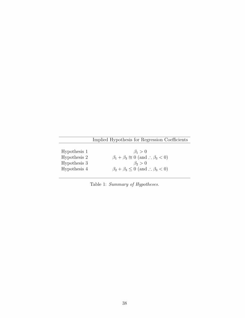
Implied Hypothesis for Regression Coefficients

Hypothesis 1 β1 > 0Hypothesis 2 β1 + β3 u 0 (and ∴ β3 < 0)Hypothesis 3 β2 > 0Hypothesis 4 β2 + β3 ≤ 0 (and ∴ β3 < 0)

Table 1: Summary of Hypotheses.

38

Regressor Full Sample Presidential RegimesRunoff (β1) 2.201 2.017

(0.299) (0.500)0.000 0.001

AGT2/3 (β2) 1.315 1.547(0.309) (0.469)0.000 0.004

Runoff *AGT2/3 (β3) -2.519 -2.923(0.496) (0.726)0.000 0.001

Constant (β0) 1.953 1.953(0.094) (0.099)0.000 0.000

Standard Error of Regression 1.188 0.925R-squared 0.166 0.387Observations 49 23

Table 2: Effective Number of Presidential Candidates, 1990s Cross-section. Each cell reportsOLS coefficient estimates, their robust standard errors (in parentheses), and p-values for theregression of ENPRES on Runoff, AGT2/3, and their interaction.

39

Regressor Full Sample Presidential RegimesRunoff (β1) 1.618 1.437

(0.273) (0.368)0.000 0.001

AGT2/3 (β2) 0.982 1.352(0.315) (0.371)0.000 0.001

Runoff *AGT2/3 (β3) -1.772 -2.247(0.437) (0.564)0.000 0.001

Constant (β0) 2.003 2.003(0.100) (0.102)0.000 0.000

Standard Error of Regression 1.136 0.993R-squared 0.079 0.207Observations 101 51

Table 3: Effective Number of Presidential Candidates, 1990s Pooled. Each cell reports OLScoefficient estimates, their country clustered robust standard errors (in parentheses), and p-values for the regression of ENPRES on Runoff, AGT2/3, and their interaction.

40

Appendix: Proofs of Propositions

Proof of Proposition 1. Any group A (B) citizen who fails to enter when her group doesnot have a candidate violates the behavioral prescription against harming the group’s electoralperformance, incurring a sufficiently large cost that there is always an incentive to enter. So(0, n) and (n, 0) are not possible for any n. ¥

Proof of Proposition 2. In any (1, n) setting, candidate A wins regardless of her policy,which is unconstrained by B candidates’ choices. Given this and since n > 1, B candidates willonly have an incentive to stay in if they win a share of group leadership. As such, in any (1, n)equilibrium, there must be an n-way tie among group B candidates. An A citizen at the idealpoint of the A “incumbent” could enter and tie the election without affecting the winning policy(since n ≥ 2 and A > B, A/2 > B/n) earning utility γ/2 − c > 0, so there is an incentive toenter and (1, n) is not possible for n > 1. ¥

Proof of Proposition 3. First suppose A ∈ (12, 2

3). For (1, 1) equilibrium existence, the (i)

A and (ii) B candidates must wish to stay in, and no other (iii) A or (iv) B candidates must wishto enter. (i) and (ii): Along with the fact that there can be no identity reason for a solo groupcandidate to exit, γ > c (g(B) > c) implies the A (B) candidate won’t drop out. (iii) There isno identity incentive for A entry. Suppose the A candidate’s policy is at the median A voter.Then a potential A entrant must always lose, either to incumbent A (paying entry cost with nopolicy or winning benefit), or to the B candidate (suffering lexicographic identity losses), sinceB > A

2. So an A incumbent at the A voter median can deter entry by A citizens. (iv) There

is no identity incentive for B entry. Suppose the B candidate is at the median B voter. Then apotential B entrant can do no more than tie for group B support, without affecting policy, whichwill not be worth the cost of entry so long as c > g(B)

2. Thus (i)-(iv) can be simultaneously

satisfied and so (1, 1) is possible. Now suppose A ∈ (23, 1). Now an A citizen who shared the

incumbent A’s policy would be able to enter and win vote share A2, tying for first since now

A2

> B. Since γ2

> c there will be an incentive to enter so (1, 1) is not possible. ¥Proof of Proposition 4. In a (2, 1) setting, if the two A candidates are not tied, then

the trailing candidate, who pays entry costs but does not influence policy or receive winningbenefits, will drop out because there will never be identity costs for doing so. So if (2, 1) ispossible, it must involve a tie between the two A candidates.

Suppose that A ∈ (12, 2

3). Each A candidate wins vote share A

2< B, so B wins the race

and either A candidate would wish to exit for identity reasons to ensure victory for the other Acandidate. So (2, 1) is not possible. Now suppose A ∈ (2

3, 1). For (2, 1) equilibrium existence,

the (i) A and (ii) B candidates must wish to stay in, and no other (iii) A or (iv) B candidatesmust wish to enter. (i) and (ii): Because there are clearly no identity reasons for exit, as exitwould improve neither group vote share nor the probability of group victory, and because the Acandidates tie with vote share A

2> B, γ

2> c (g(B) > c) implies the A (B) candidates wouldn’t

drop out. (iii) There are clearly no identity incentives for A entry. Because they must tie, thetwo A candidates must be symmetrically spaced around the median A voter; they cannot be atthe same position, since an arbitrarily close potential A entrant could get at least arbitrarilyclose to half of the A vote (because the distribution of ideal points is continuous), and win sinceA2

defeats the B candidate. In Proposition 2 of Osborne and Slivinski, two incumbents spacedaround a median voter can deter entry by a citizen who cares about winning and policy in the

41

same way that ours do; the competition by group A candidates for group A voters takes on thesame form here, except that additional constraints are imposed (for example, winning group Adoes not imply victory, as one must also defeat group B candidates in order to win). As suchtheir deterrence result implies that all potential A entrants can be deterred here as well. (iv)There are clearly no identity incentives for B entry. Suppose the B candidate is positioned atthe median B voter. Then a potential B entrant can do no more than tie for group B support,without affecting policy or identity, which will not be worth the cost of entry so long as c > g(B)

2.

Note that (i)-(iv) can be simultaneously satisfied; so (2, 1) is possible. ¥Proof of Proposition 5. In a (2, 2) setting, if the two A candidates are not tied, then

the trailing candidate, who pays entry costs but does not win or influence policy, would pay noidentity costs for exiting, and will wish to. So any equilibrium must involve a tie between thetwo A candidates. Further, because either A candidate could ensure the victory of the other bydropping out, A identity concerns imply that all B candidates lose for sure in equilibrium. Giventhis and since there are multiple B candidates, B candidates can be motivated only by groupleadership payoffs, as their policies have no effect on the A candidates. As any B candidate nottied for the lead would then wish to drop out, both group B candidates must win vote share B

2.

For (2, 2) equilibrium existence, the (i) A and (ii) B candidates must wish to stay in, and noother (iii) A or (iv) B candidates must wish to enter. (iv) There can be no identity motivationfor B entry as all A candidates beat all B candidates. Since B entrants cannot affect policyoutcomes, entry incentives are limited to B group leadership. The only way for tied B candidatesto deter entry is with candidates symmetrically spaced about the median. (ii) There will beidentity incentives to drop out if this increases the probability of a B candidate victory. For(2, 2) this is true if B > A

2, that is A < 2

3. If there is no such identity incentive then candidates

will wish to stay in so long as g(B)2

> c. (i) The A candidates tie for the win for sure, so thereare no identity reasons for exit. Further, γ

2> c ensures that neither A candidate will wish to

exit. (iii) By the same logic as in part (iii) of the proof of Proposition 4, it is possible to deterentry by further A citizens. Note that (i)-(iv) can be simultaneously satisfied, and equilibriaare therefore possible, when A > 2

3for (2, 2). ¥

Proof of Proposition 6. (3, 1) configurations potentially involve: (1) An A candidatewins outright; (2) Two or more A candidates tie for the win; (3) An A candidate and the Bcandidate tie for the win; (4) Two or more A candidates and the B candidate tie for the win;and (5) the B candidate wins outright. But in (4), at least one of the A candidates would wishto drop out for identity reasons, to increase the probability of an A candidate winning. And in(1) or (3), there are two A candidates who lose outright, and who therefore do not share thewinning A’s policy. If the losing A’s share the same policy, either of these will wish to drop out,whereas if they do not share the same policy, at least one of them (and possibly both) mustnot be the centrist candidate and will wish to drop out because they experience no winning,policy, or identity benefit from entry. If (5), the B candidate wins outright, and the losing Acandidates do not even influence policy, so to stay in they must win some group leadershipbenefit and not wish to exit for identity reasons. Because of the former all three A candidatesmust receive vote share A

3. There are three ways the A candidates could tie: (I) all have the

same policy; (II) exactly two candidates share the same policy; (III) all have different policies.Case I cannot form the basis for an equilibrium, because there must exist a potential A entrantwho can win a vote share that is at least arbitrarily close to A

2by continuity of F, which would

42

give benefit g(A) > c and therefore an incentive to enter. For both cases II and III, the largestvote share for the new A vote-winner after one candidate exits is 2A

3(for case II, when one of

the coincident A candidates exits; for case III, when either of the A candidates who are at the“extremes” exits). If the vote share for the top A candidate exceeds B, then the A candidatewins; as such, there can be no identity incentive for exit only when 2A

3< B, or A < 3

5. Now

consider a potential B entrant at the ideal point of the B incumbent candidate. Tying for firstin an election is always worthwhile (γ

2> c), so such entry entrant can only be deterred if it

would cause the now-tied B group candidates to place below the A candidates, i.e. if B2

< A3

orA > 3

5. As this is incompatible with the condition above, no equilibrium corresponds to cases

II or III, and therefore to (5). This leaves (2), which is not feasible for all A: specifically, two Acandidates can tie for the win only if A ∈ (2

3, 1), whereas three A candidates can tie for the win

only if A ∈ (34, 1) because the B candidate must win vote share 1 − A. The B candidate will

wish to remain in the race for identity reasons (or simply because g(B) > c), and as B citizenshave no identity or policy incentive to enter, they can be deterred from entry, for example if theB incumbent is at the median B voter and if c > g(B)

2. There is no identity incentive for A entry,

and Proposition 3 of Osborne and Slivinski is sufficient to demonstrate that further A citizenscan be deterred from entering for policy or winning reasons for either the two-way or three-waytie cases, since entrants in our models not motivated by identity must meet their conditions(as well as further constraints that are not necessary to consider). Finally, there is no identityincentive for A exit, and Proposition 3 of Osborne and Slivinski demonstrates that the furthernecessary and sufficient conditions can also be met. So (3, 1) is possible for any A ∈ (2

3, 1) and

the possible equilibrium vote shares are as described. ¥Proof of Proposition 7. Same logic as in the corresponding plurality case. ¥Proof of Proposition 8. For n > 1, the proof is almost identical to that in the corre-

sponding plurality case (Proposition 2). For n = 1, consider a potential group A entrant whoshares the incumbent A candidate’s ideal point. If she enters, she wins vote share A

2in the first

round. There are then three cases for the first round depending on A: (1) the A candidatestie for first; (2) the A candidates tie for second; and (3) all candidates tie for first. In (1), thetwo A candidates both advance to a runoff, which is also tied; each wins with probability 1

2.

In (2), each of the A candidates advances to (and then certainly wins) a runoff against B withprobability 1

2. In (3), with probability 1

3, the two A candidates both advance to the runoff, which

each wins with equal probability; in addition, each of the A candidates advances to (and thencertainly wins) a runoff against B with probability 1

3. In all three cases, the entrant wins with

probability 12. Because A candidate(s) always win(s) the election and maximum possible vote

share regardless of entry, there are no identity costs or benefits to entry; and because here theA candidates share the same policy position, there are no policy costs or benefits to entry. Theentry condition is then just γ

2− c > 0, which is true by assumption. So (1, 1) is not possible. ¥

Proof of Proposition 9. Take A ∈ (12, 2

3). For (2, 1) equilibrium existence the (i) A and

(ii) B candidates must wish to stay in, and no other (iii) A or (iv) B candidates must wishto enter. (i) and (iii): The B candidate wins vote share (1 − A) ∈ (1

3, 1

2) in the first round,

earning no worse than second place, so the B candidate always makes it to the runoff against oneultimately victorious A opponent. Thus, being the top first-round A candidate is tantamountto election, and the strategic problem facing A candidates in the first round of the runoff systemin a divided society is exactly the same as the one they would face in a plurality system in which

43

the A group comprised the entire electorate. As such, Proposition 2 of Osborne and Slivinski,along with the observation that there are no identity reasons for A exit or entry, demonstratethat (i) and (iii) can can both be satisfied. (ii) The B candidate will clearly not wish to exitbecause g(B) > c as well as for identity reasons. (iv) Group B entrants could be motivatedeither by group leadership concerns (which can be deterred by a B incumbent at the median B

voter if c > g(B)2

) or by identity concerns. A solo B candidate in a runoff always loses; identity-motivated entry can occur here if and only if it leads both the B candidates to at least tie thetop A candidate in the first round. The most efficient (and always feasible) allocation of B votesis to divide them equally between the B candidates, so deterrence of this case is necessary andsufficient for condition (iv). Since A candidates must tie in (2, 1), the deterrence condition isB2

< A2, which holds since A > B.

Now take A ∈ (23, 1). Clearly the B candidate cannot tie or beat both of the A candidates.

And, any A candidate trailing B does not make the runoff, so would wish to drop out to saveentry costs. So either (1) both the A’s beat the B in the first round or (2) one of the A’s beatsthe B while the other ties. Two A candidates in a runoff must tie in the runoff, or the trailingcandidate would drop out; so the A’s either have the same policy or are symmetrically arrangedaround the overall median voter. An A always wins the election. For (2, 1) equilibrium existencethe (i) A and (ii) B candidates must wish to stay in, and no other (iii) A or (iv) B candidatesmust wish to enter. (i) There are clearly no identity reasons for A exit. For (1), γ

2> c implies

that there will be no incentive for exit; for (2), this will still be true so long as γ4

> c. (ii) Theincumbent B candidate will clearly not wish to exit because g(B) > c and for identity reasons.(iv) If the B incumbent is at the median B voter, all potential B entrants can be deterred so

long as c > g(B)2

, as there are no identity motivations for entry in a situation where the sole Bcandidate was no better than tied for second to begin with. (iii) Consider (1). Suppose that theA incumbents have positions symmetric about the overall median voter. There are no identityincentives for entry since an A candidate always wins the election. For entry at a position thatis either to the left or to the right of both A incumbents, there can be no policy incentive sinceentrants drain votes only from the incumbent whose policy the entrant prefers. An A incumbentwould still make the runoff for sure, and would beat any such entrant who also made the runoffbecause of distance from the median voter. By familiar logic, it is also possible to deter entrybetween the two A incumbents; if the incumbents are sufficiently close together, such entrantswould fail to make the runoff or change the composition of the candidates who do make therunoff. The remaining possibility is of a potential entrant at the policy of one of the incumbentcandidates. An entrant at the policy of candidate Aj will receive vote share

Aj

2; clearly the entry

incentive will be at least as great at x1 as at x2 if A1 ≥ A2 (which we assume without loss ofgenerality). If A1 < 2A2, such an entrant would finish no better than a two-way tie for second inthe first round: this best case scenario leads to a runoff place with probability 1

2, and conditional

on that a victory with probability 12, for a best-case victory probability of 1

4, and no impact on

the probability distribution of policy outcomes, so that there will be an incentive to enter if andonly if γ

4> c. As such, in this case, entry can be deterred if γ

2> c > γ

4. (If the entrant does

worse than a two-way tie for second place, the expected winning and policy benefits of entrywill both be at least weakly worse, so deterrence will be possibly for a weakly wider range ofconditions.) If A1 = 2A2, then the entrant would be tied for first place among the A candidates,with an expected winning benefit γ

3and an improved distribution of policy outcomes for the

44

entrant. The deterrence condition here is γ2

> c > γ3

+ δ6

which is clearly possible if the policyseparation δ between the A incumbents is not too large. Finally, if A1 > 2A2, then the entrantwould be tied for first, and win the runoff with probability 1

2, so that there would always be

an incentive for entry since γ2

> c. So in this case, entry cannot be deterred at all. As such,for (1), A entrants can be deterred as long as A1 ≤ 2A2. (Therefore to determine the voteshares that are possible in equilibrium, considering A incumbents with identical positions isnot necessary since A1 = A2 is already included here.) Now consider (2), with first-round voteshares A1 > A2 = B. Entry at the extremes of A1 and A2 and at x1 and x2 involve the sameconsiderations and thus deterrence conditions as above. Entry in between A1 and A2 is notthe same because now an infinitesimal measure of support garnered between A1 and A2 couldpotentially change the vote share orderings. Now suppose that all A2’s support comes from her“extreme” flank away from A1, that A1 gets from her “extreme” flank support less than A2, thatA1’s “centrist” support is at least three times closer to x1 than to x2, and that x1 and x2 aresufficiently close. Then there is no incentive for entry in between the incumbents (no chance towin since policies sufficiently close; and entrants cannot achieve policy improvements since therelevant voters are out of reach). So the conditions are the same in (2) as in (1). Thus, (i)-(iv)can be simultaneously satisfied, so (2, 1) is possible under the conditions described. ¥

Proof of Proposition 10. An A candidate must win the election for sure; otherwise eitherA candidate would wish to drop out for identity payoff reasons. As such, the B candidatesmust tie each other; otherwise, trailing B candidates would wish to drop out, because groupleadership payoffs provide the only incentive for entry. Also, an A candidate with no chanceof winning would drop out, so both A candidates must make the runoff with some probability.And at least one A must be in the runoff every time as an A candidate must win for sure: soeither (1) both A’s beat the B’s, or (2) one A beats the B’s while the other A ties the B’s.If both A candidates advance to the runoff, they must tie in the runoff (or one would wish toexit). For (2, 2) equilibrium existence the (i) A and (ii) B candidates must wish to stay in,and no other (iii) A or (iv) B candidates must wish to enter. (iv) There can be no identitymotivation for B entry as all A candidates beat or tie all B candidates in the first round. SinceB entrants cannot affect A policy choices, entry incentives are limited to B group leadership.The only way for tied B candidates to deter such entry is with candidates symmetrically spacedabout the median. (ii) Identity motivations for exit can exist only if a B candidate’s exit createspositive probability that two B candidates will simultaneously qualify for the runoff (if only oneB candidate is in the runoff, she would lose for certain). For (2, 2) this cannot exist because exit

leaves only one B candidate. As such, B candidates will not exit so long as g(B)2

> c. (i) Therecan be no identity incentive for A exit. If the two A candidates both defeat the B’s outright,γ2

> c implies there will be no incentive for exit; if one of the A candidates ties the B’s, it isnecessary and sufficient that γ

6> c, because this candidate makes the runoff with probability 1

3

and conditional on that wins half the time. So it is possible for both A candidates to wish tostay in for either of cases (1) and (2). (iii) The argument in part (iii) of the proof of Proposition9 for A ∈ (2

3, 1) holds here, replacing B in that proof with B

2here. Note that (i)-(iv) can be

simultaneously satisfied, so (2, 2) is possible under the conditions described. ¥Proof of Proposition 11. For A ∈ (1

2, 2

3), the argument in Proposition 9 for (2, 1),

A ∈ (12, 2

3), holds here except that the relevant reference in Osborne and Slivinski (“OS”) is

Proposition 3, and the deterrence condition for B entry is instead B2

< A3, or A > 3

5, for the

45

three-way tie specified in OS Proposition 3, and B2

< xA, or A > 12x+1

for the two-way tie (two A

candidates get xA, x ∈ (13, 1

2), while the third trails with (1− 2x)A). Note 1

2x+1∈ (1

2, 3

5) so that

for the two-way tie A can take on any value between 12

and 23, as long as x ∈ (max(1

3, 1

2A− 1

2), 1

2).

Now take A ∈ (23, 1). Taking A candidate vote shares A1 ≥ A2 ≥ A3, there are 20 different

relative orderings (including potential indifference) of these vote shares along with that of theB candidate. The six with A1 and A2 unambiguously as the top two cannot be in equilibrium;if the last-placed A candidate exited, it would not affect who made the runoff, and thereforenot affect policy, nor does the trailing A get identity or winning gains from staying in. The sixwith A1 and B unambiguously as the top two also cannot be in equilibrium. A2 and A3 do notget winning or identity benefits from running, since an A candidate ultimately wins regardless,so only policy reasons could keep them from exiting. Only a candidate in the middle of threedispersed candidates could have such an incentive; extreme or coincident candidates can onlydraw support away from their most favored alternative. But clearly A2 and A3 cannot both bethe central of three dispersed candidates, so at least one must wish to exit.

We consider the eight remaining orderings in turn. In each instance, the incumbent Bcandidate will not wish to withdraw because of identity reasons (and g(B) > c), and potentialB entrants can be deterred, since there is no identity motive for entry (both B candidates cannotmake the runoff since for A > 2

3, B

2< A

3), if the B incumbent is at the median B voter, so long

as g(B)2

< c. As such we consider only A candidate incentives below.Three remaining orderings involve: (1) three A candidates tie for first place (A > 3

4); (2)

all four candidates tie for first place (A = 34); and (3) three A candidates tie for second place

(A < 34). In their Proposition 8, OS describe alternative policy configurations leading to this

vote share; to demonstrate existence here, it is sufficient to focus on a runoff equilibrium inwhich all three A candidates have different positions but win equal vote shares, and in whichthe two extreme candidates are symmetric about the (overall) median voter. Consider A exitincentives, noting there is no identity incentive for exit since an A always has to win. For(1), the analysis is identical to OS, and demonstrates that the entrants don’t exit for γ

6> c.

For (3), the A candidates compete for only one runoff spot. Each gets it with probability 13,

and after getting it, beats B in the runoff. So there will be no exit incentive here so long asγ3

> c. For (2), each of the A candidates competes in three of six possible runoff pairings; thecentral (non-central) candidate(s) win all of them (win one, tie one, and lose one), with no exitincentive so long as γ

2> c (γ

4> c). Now consider incentives of potential A entrants. There are

no identity-related motives for entry. OS show in their setting that entrants whose objective isto finish first or second among the A candidates can be successfully deterred. This is sufficientto show entry deterrence is possible here for (1), (2), and (3).

Two further orderings are (4) A1 > A2 = A3 > B and (5) A1 > A2 = A3 = B. Consider x1

and x2 symmetric about the overall median voter, with x1 < x3 < x2. Further suppose that thedistribution of A1 voters has support [y, x1], y < x1; the distribution of A2 voters has support[x2, z], z > x2; and all A3 voters are contained within (3x3+x1

4, 3x3+x2

4). Here A1 is always in

the runoff. When A1 > 2A2, there is clearly no means of deterring entry (as an entrant atx1 can win with probability 1

2and ensure her ideal policy), so we restrict our attention to the

complementary cases. In (4), A1 faces either of the other A candidates; A1 ties A2 but losesto A3 in runoff matchups, so that A1 and A2 (A3) win with probability 1

4(1

2). In (5), A1 faces

any of the other three candidates, beating B, tying A2, and losing to A3, so A1 (A2) {A3}

46

win with probabilities 12

(16), and {1

3}. For (4,5), one can write conditions for non-exit for all

three A candidates in terms of these probabilities and the probabilities of victory that wouldhold if the candidates individually dropped out (which are clearly determined by the preferencedistribution described); γ; c; and the policy distances between candidates, which can clearly besatisfied simultaneously when γ is large enough relative to c and potential policy costs of entry.(Note also that the conditions for B can also be simultaneously satisfied.) For A entry, for thegiven preference distribution, no entrant can win or obtain identity benefit, and entrants whoare able to win positive vote shares take them from their most favored candidate and thereforeobtain no policy benefit. This establishes that A entry can be deterred for general (4) and (5)if and only if A1 < 2A2.

The final three orderings are (6,7) B ≥ A1 = A2 > A3 and (8) A1 > A2 = B > A3. For(8), A3 must clearly prefer the policy of A1; if A3 instead preferred the policy of A2, she couldnot harm but might help A2’s prospects by dropping out of the race, and so would not wishto pay the costs of entry. Similarly label as A1 the candidate whose policy A3 prefers in (6,7)(without loss of generality). Consider x1 and x2 symmetric about the overall median voter, withx1 < x3 < x1+x2

2< x2. Note first that for (8), as above, entry cannot be deterred if A1 > 2A2,

so we take A1 < 2A2 (automatically true for (6,7)). Consider then a preference distribution forwhich vote share less than A2 lies left of x1; vote share less than A2 lies right of x1 but left of3x1+x3

4; vote share y < A2−A3 lies right of x2 while A2−y lies left of x2 but right of x3+3x2

4; and

vote share A3 lies on [x1+x2

2, z] for some z < 3x3+x2

4. In (6,7), A1 and A2 each win with probability

12

while in (8) A1 (A2) wins with probability 34

(14). For (6,7,8), one can write conditions for

non-exit for all three A candidates in terms of these probabilities and the probabilities of victorythat would hold if the candidates individually dropped out (which are clearly determined bythe preference distribution described); γ; c; and the policy distances between candidates, whichcan clearly be satisfied simultaneously when c is small enough relative to the policy distances(so that A3 will wish to enter to influence policy) and when γ is large enough relative to c andpotential policy costs (for A1 and A2) of entry. (Note also that the conditions for B can also besimultaneously satisfied.) For A entry, for the given preference distribution, no entrant can makethe runoff or obtain identity benefit, and entrants who are able to win positive vote shares takethem from their most favored candidate and therefore obtain no policy benefit. This establishesthat A entry can be deterred for general (6), (7), and (8) if and only if A1 < 2A2. ¥

47