Social Learning and Incentives for Experimentation and Communicationⱡ

Ariel BenYishay, College of William & Mary

A. Mushfiq Mobarak, Yale University

March 2017

Abstract

Low adoption of agricultural technologies holds large productivity consequences for developing countries. Many countries hire agricultural extension agents to communicate with farmers about new technologies, even though a large academic literature has established that information from social networks is a key determinant of product adoption. We incorporate social learning in extension policy using a large-scale field experiment in which we communicate to farmers using different members of social networks. We show that communicator own adoption and effort are susceptible to small performance incentives, and the social identity of the communicator influences others’ learning and adoption. Farmers appear most convinced by communicators who share a group identity with them, or who face agricultural conditions most comparable to themselves. Exploring the incentives for injection points in social networks to experiment with and communicate about new technologies can take the influential social learning literature in a more policy-relevant direction.

Keywords: Social learning, Technology Adoption, Agriculture, Peer Effects

JEL Codes: O33, O13, Q16

ⱡ Contact: BenYishay: abenyishay@wm.edu, or Mobarak: ahmed.mobarak@yale.edu. We gratefully acknowledge the support and cooperation of Readwell Musopole and many other staff members of the Malawi Ministry of Agriculture, and of David Rohrbach and Olivier Durand of the World Bank – Malawi Country Office. Maria Jones managed all aspects of fieldwork extremely well. Niall Kelleher, Sylvan Herskowitz, Cristina Valverde and the IPA-Malawi country office provided invaluable support for data collection. Andrew Carter, Tetyana Zelenska, Johann Burnett and Imogen Halstead provided excellent research assistance. The World Bank Gender and Agriculture Program, World Bank Development Impact Evaluation Initiative (DIME), the Millennium Challenge Corporation, Yale Center for Business and Environment, and the Macmillan Center at Yale University provided financial support. We thank Francesco Caselli, four anonymous referees, Chris Udry, Florian Ederer, Jonathan Feinstein, Arthur Campbell, Ken Gillingham, Florence Kondylis, Arik Levinson, Mark Rosenzweig, and seminar participants at Yale University, University of Michigan, Brown University, Boston University, Boston College, Georgetown, University of Warwick, University of Cambridge, Vassar College, the College of William & Mary, the University of Sydney, Monash University, University of Queensland, the University of New South Wales, Stanford University SITE, NEUDC at Harvard, and the 24th BREAD conference for comments. All errors are our own.

1     

1. Introduction

Many agricultural technologies with demonstrated productivity gains, such as timely fertilizer

application, improved seed varieties, and composting, have not been widely adopted in developing

countries, and in Sub-Saharan Africa in particular (Duflo, Kremer and Robinson 2011, Udry 2010).

The 2008 World Development Report vividly documents the associated costs – agricultural yields

and productivity have remained low and flat in sub-Saharan Africa over the last 40 years (World

Bank 2008). Investing in new technologies is risky, and lack of reliable and persuasive sources of

information about new technologies, their relevance to local agronomic conditions, and details on

how to apply them, are potential deterrents to adoption.1 Farmers care about the expected

performance of the technology at their own plot of land, and the social proximity, relevance and

credibility of the source of the information may therefore matter.

The economics and sociology literatures have long recognized the importance of social

learning from peers in overcoming such “information failures” in both developed (Griliches 1957,

Rogers 1962) and developing (Foster and Rosenzweig 1995, Bandiera and Rasul 2006, Conley and

Udry 2010) countries. This literature has largely focused on documenting the existence of social

learning using careful empirical strategies.2 These models explore a ‘passive’ form of social learning,

implicitly assuming that farmers costlessly observe the field trials of their neighbors with little

friction in the flow of information, and then update their expectations about the technology’s

profitability. Now that the importance of social learning has been established, a natural next

question is whether the power of social influence can be leveraged to promote new technologies.

                                                            1 Other deterrents examined by the literature recently include imperfections in credit markets (Croppenstedt, Demeke and Meschi 2003, Crepon et al 2011), insurance markets (Cole, Giné and Vickery 2013, Bryan, Chowdhury and Mobarak 2014, Karlan et al 2012), land rights (Goldstein and Udry 2008, Ali, Deininger, and Goldstein 2011), and output markets (Ashraf, Giné, and Karlan 2009). Jack (2013) offers a careful review of this literature. 2 Distinguishing peer effects from incidental correlations in the behavior of social contacts has been the perennial empirical challenge with which this literature has grappled (Manski 1993). A growing literature shows that social relationships are an important vector for the spread of information in a variety of contexts, including educational choices (Garlick 2012; Bobonis and Finan 2009; Carrell and Hoekstra 2010; de Giorgi et al 2010; Duflo, Dupas, and Kremer 2011), financial decisions (Burzstyn et al 2014; Banerjee et al. 2013; Beshears et al, 2011; Duflo and Saez 2003), job information (Beaman 2012; Magruder 2010), health inputs (Kremer and Miguel 2007, Godlonton and Thornton 2012, Oster and Thornton 2012; Miller and Mobarak 2015), energy choices (Alcott 2011) and doctors prescribing drugs (Coleman et al. 1957, Iyengar et al 2011).  

2     

Our study explores whether we can cost-effectively improve new technology adoption by

involving farmers closer to the target population as promoters, and by providing them incentives

to experiment with the technology and communicate this information to others. We do this

through a randomized control trial (RCT) in which we vary the dissemination method for two new

technologies for maize farming across 168 villages in Malawi. In each village, we randomly assign

the role of main communicator about the new technology to either (a) a government-employed

extension worker, (b) a ‘lead farmer’ (LF) who is educated and able to sustain experimentation

costs, or (c) five ‘peer farmers’ (PF) who are more representative of the general population and

whose experiences may be more applicable to the average recipient farmer’s own conditions.

Random subsets of these communicators are offered small performance-based incentives in the

experimental design.3

We first document that providing incentives to communicators affects the flow of

information in these villages. Without incentives, PFs and LFs rarely adopt the technologies

themselves, and largely do not communicate information about the technologies to target farmers.

As a result, target farmers do not know more about the technologies or adopt them at higher rates

than in control communities. In contrast, when incentivized, PFs and LFs experiment at higher

rates and communicate information to other farmers, who subsequently adopt the technology

themselves. There is greater diffusion of knowledge and adoption by target farmers when PFs are

incentivized, especially for the more novel of the two technologies.

These incentive results imply that when we try to use social influence to promote new

technologies, experimentation and transmission of information to others cease to be automatic.

This is a crucial difference between the passive social learning documented by Griliches (1957) and

                                                            3 Our work relates to recent studies that promote new technologies through network ‘injection points’: Kremer et al 2011, Ashraf, Bandiera and Jack 2012, Leonard and Vasilaky 2014, Beaman et al 2015. A literature in medicine has explored the role of opinion leaders in changing behavior (Kuo et al 1998, Locock et al 2001, Doumit et al 2007, Keating et al 2007). A marketing literature explores conditions under which incentives stimulate word-of-mouth referrals (Biyalogorsky, Gerstner, and Libai 2001; Kornish and Li 2010). Also related, more broadly, is the lengthy literature on the effects of performance-based incentives on the production of public goods, reviewed by Bowles and Polania-Reyes (2012).  

3     

others (in which some farmers experiment with technologies on their own, neighbors learn by

observing them, and ideas slowly diffuse), and the social diffusion of a new technology we try to

“activate” via a policy intervention. Diffusion through an external intervention appears to follow

a different process, and may require us to pay more careful attention to early adopters’ incentives

for experimentation and for communicating information to others. When communicator

incentives are added, we observe a brand new technology move from essentially zero market

penetration to about 10-14% usage within two agricultural seasons.

We provide an informal conceptual framework that explains (1) why incentives matter in

this setting, and (2) why peer farmers may react more strongly to incentives.4 This generates

auxiliary testable predictions that allow us to delve deeper into the questions of communicator and

target farmer characteristics that lead to faster adoption. The greater effectiveness of PFs that we

document could stem from their greater social or physical proximity to target farmers, but our data

indicate that similarity in farm size and input use, and common group membership matter more.

Farmers appear to be most convinced by the advice of others who face agricultural conditions that

are comparable to the conditions they face themselves.5 We do not attempt to influence specific

actions by peer farmers, but we document strategies they use. Incentives induce peer farmers to

both expend communication effort and adopt the technology themselves, and the latter has a

demonstration effect.

For policy, our results suggest that social learning can be harnessed to cost-effectively

improve public agricultural extension services. Adoption of our targeted technologies increased

maize yields substantially, making the incentive-based communication strategies cost-effective.

More broadly, while large numbers of extension workers are employed in developing countries

                                                            4  Our work relates to the theoretical literature on incentives for communication of non-verifiable information (beginning with Crawford and Sobel 1982) and verifiable information requiring effort on the part of senders and receivers (Dewatripont and Tirole 2005). Our experiment varies types of senders who have different effort costs, and introduces incentives that change the sender’s stake in the communication.  5 This is consistent with results from both psychology (Briñol and Petty 2009, Fleming and Petty 2000) and economics (Munshi 2004) on the role of similarity between senders and receivers of information in persuading the latter to adopt specific behaviors. 

4     

(Anderson and Feder 2007), the impact of these services have largely been disappointing: the use

of modern varieties of seeds, fertilizer, and other agricultural inputs has remained relatively

stagnant and unresponsive to extension efforts in sub-Saharan Africa (Udry 2010, Krishnan and

Patnam 2013). These deficiencies can often be traced back to a lack of qualified personnel and

insufficient resources,6 suggesting that cost-effectively leveraging social networks may be a

particularly powerful way to address these failures.

This paper is structured as follows: Section 2 describes the context and experimental

design. Section 3 presents a conceptual framework for social learning with endogenous

communication. The data are described in Section 4 and empirical results presented in Section 5.

We test for alternative mechanisms underlying our results in Sections 6 and 7. We study the

impacts on target farmers’ yields and inputs in Section 8, and offer concluding remarks about

policy implications in Section 9.

2. Context and Experimental Design

Our experiment takes place in eight districts across Malawi. Approximately 80% of Malawi’s

population lives in rural areas, and agriculture accounts for 31% of Malawi’s GDP (World Bank

2011). Agricultural production and policy is dominated by maize.7 More than 60% of the

population’s calorie consumption derives from maize, 97% of farmers grow maize, and over half

of households grow no other crop (Lea and Hanmer 2009). The maize harvest is thus central to

the welfare of the country’s population, and has been subject to extensive policy attention.

The existing agricultural extension system in Malawi relies on government workers who

both work with individual farmers and conduct village-wide field days. These Agricultural

Extension Development Officers (AEDOs) are employed by the Ministry of Agriculture and Food

                                                            6 Approximately 50% of government extension positions remain unfilled in Malawi, and each extension worker in our sample is responsible for 2450 households on average. The shortage of staff means that much of the rural population has little or no contact with government extension workers. According to the 2006/2007 Malawi National Agricultural and Livestock Census, only 18% of farmers report participating in any type of extension activity. 7 While there has been some recent diversification, the area under maize cultivation is still approximately equivalent to that of all other crops combined (Lea and Hanmer 2009). 

5     

Security (MoAFS). These workers are notionally responsible for one agricultural extension section

each, typically covering 15-25 villages (although given the large number of vacancies, AEDOs are

often in fact responsible for multiple sections). Section coverage information provided by MoAFS

in July of 2009 indicated that 56% of the AEDO positions in Malawi were unfilled.

Partly in response to this shortage, MoAFS had begun developing a “Lead Farmer”

extension model, in which AEDOs would be encouraged to select and partner with one lead

farmer in each village. The aim was to have these lead farmers reduce AEDO workload by training

other farmers in some of the technologies and topics for which AEDOs would otherwise be

responsible. We incorporate this lead farmer model in our experimental design.

No formal MoAFS guidance existed on the use of other types of partner farmers to extend

an AEDO’s reach (or reduce his workload). We introduce a new extension model: the AEDO

collaborating with a group of five peer farmers in each village, who are selected via a village focus

group and are intended to be representative of the average village member in their wealth level and

geographically dispersed throughout the village.

2.1. Experimental Variation in Types of Communicators

We designed a multi-arm study involving two cross-cutting sets of treatments: (1) communicator

type, and (2) incentives for dissemination. We randomized assignment into these treatments at

the village level. Each village was randomly assigned to one type of communication strategy:

(a) AEDO only

(b) Lead Farmer (LF) - supported by AEDO

(c) Peer Farmers (PFs) - supported by AEDO

In all three arms, the AEDO responsible for each sampled village was invited to attend a

3-day training on a targeted technology relevant for their district (discussed below). In each of the

two farmer-led treatments, the AEDO was then to train the designated LF or PFs on the specific

technology, mobilize them to formulate workplans with the community, supervise the workplans,

6     

and distribute technical resource materials (leaflets, posters, and booklets). Appendix A1 provides

some additional details.

Guidance given to AEDOs specified that LFs selected should have the following characteristics:

(A) Identified by the community as a “leader”

(B) Early adopter of technology

(C) Literate

(D) May have more resources at his/her disposal to aid technology adoption (oxcart, access to

chemical fertilizers or pesticides, more land)

The selection process involved the AEDO convening a meeting with community members to

identify a short list of potential lead farmers. The AEDO selects one of the farmers on the short

list to be the lead farmer, in consultation with village leaders, and was then asked to announce his

choice to the village, to ensure that the community endorses the new lead farmer.

Guidance given to AEDOs specified that PFs selected should have the following characteristics:

(A) Thought of by the community as ordinary, average farmer

(B) Must be willing to try the new technology, but is not necessarily a progressive farmer

(C) Not necessarily literate

(D) Similar to average farmers in the village in terms of access to resources.

The selection process for PFs again involved the AEDO convening and facilitating a meeting

with village members. The first step was to identify the important social groups in the village.

The directions given included (a) the meetings must be well attended (including by those who

may work with the extension agent most often), and (b) there should be representatives from all

the different social groups in the village (males, females, elders, adolescents, people from

different clubs or church groups, etc). Meeting participants from each group nominated one

representative, and the list was pared down to five in consultation with AEDOs and village

leaders. The nominated peer farmers had to state that they understood their role and

responsibilities. They were then presented to the village for endorsement.

7     

Selecting both lead and peer farmers involved village meetings, consultation with leaders

etc, and the approaches followed were not fundamentally different from each other. Furthermore,

both lead and peer farmers were identified in all villages using the selection processes described

above. However, in the villages randomly assigned to the LF (PF) treatment arm, only the selected

LF (set of PFs) was trained by the AEDO on the specific technology and given the responsibility

to spread information about the technology and carry out the prescribed workplan. Therefore,

our experimental design only varied the actual assignment of lead and peer farmers to specific

tasks, holding the selection process constant in all villages. This strategy has the additional

advantage of identifying “shadow” PFs and LFs in all villages – i.e. we know the (counterfactual)

identities of individuals who would have been chosen as PFs or LFs in all villages, had the PF or LF

treatment arm been assigned to this village. This creates an experimental comparison group for

the actual PFs and LFs, and allows us to report pure experimental effects of the treatments on an

intermediate step in the flow of information (from AEDOs to partner communicators), on the

effort expended by these communicators, and their own adoption.

We collected baseline data on all communicators to assess how the characteristics of

chosen LFs and PFs differed. Table 1 compares lead and peer farmers to each other and to the

rest of our sample (of non-communicator maize farmers who are the intended ‘recipients’ of the

messages). Lead farmers are indeed better educated and cultivate more land than both the general

population and those chosen as peer farmers. Differences in their housing quality and incomes are

also substantial but not statistically significant. Peer farmers generally fall between LFs and the

general population in all of these dimensions, and they are slightly better off than the general

population. The data therefore verifies proper implementation of the experimental design, and

motivates a key aspect of the theoretical setup: that PFs are more similar to the target farmers than

are LFs.

The PF-target farmer similarity can be an advantage to communication in multiple ways:

it could lead to greater social proximity, greater physical proximity or greater comparability in other

8     

dimensions. To investigate, Table 2 examines how LFs and PFs are perceived by, and related to,

other farmers at baseline. Using first-order links for analysis, it turns out that LFs are more central

in social networks than the average peer farmer. Respondents are significantly more likely to be

related to LFs and to talk more regularly with LFs than to each of the PFs individually. At the

same time, respondents are more likely to be related to at least one of the PFs and to talk regularly

with one of the PFs than with the LF. In other words, the five peer farmers in a village will jointly

have more links than the one lead farmer, but a one-to-one comparison suggests that LFs possess

more links. Villagers perceive LFs more favorably: they are more highly rated in terms of

trustworthiness and farming skills.8 21% of villagers report having discussed farming topics with

an LF at least several times in the previous year; only 13% of villagers have done so with the

average PF, and 9% of villagers have done so for the average non-LF/PF.

PFs do appear to have a distinct advantage in a different dimension: the average

respondent considers them to be more comparable (to themselves) in terms of farm size and input

use. At baseline, 42.7% of respondents consider the average PF in their village to have a farm size

similar to their own (compared to 33.9% for LFs), while 27.7% consider the average PF uses the

same or fewer inputs on her farm (23.1% for LF). Thus, LFs have somewhat greater social stature

than do PFs, but—partly as a result—have agricultural experiences that are further from those of

the average respondent.

The LF and PF treatment arms vary the number of communicator farmers engaged (1 LF

vs. 5 PFs) in addition to their identity. We try to disentangle communicator group size effects from

those related to identity using within-arm variation in the number of communicators per target

farmer in the village, intra-group relationships among PFs, etc, as described below.

                                                            8  These perception questions were not asked at baseline, so we rely on comparisons in our control sample to estimate differences in these characteristics.

9     

2.2. Experimental Variation in Incentives for Communicators

In addition to the random variation in communicator type, we also introduced

performance incentives for a random subset of communicators in a cross-cutting experiment. Half

of all communicators in each of the three treatment types were provided incentives conditional on

performance. Performance was defined on the basis of effects on other, recipient farmers in the

village, not the communicators’ own adoption. The ministry expected recipient farmers to hear

about the new technologies by the end of the first year (or first agricultural season), and make

actual adoption decisions only by the end of the second year. Therefore, in the first year of the

program, each communicator in the incentive treatment was told he would receive an in-kind

reward if the average knowledge score among sampled respondents in his targeted village rose by 20

percentage points. For the second year of the program, the threshold level was set as a 20

percentage point increase in adoption rates of the designated technology. We measured knowledge

by giving randomly chosen farmers in each village exams that tested whether they had retained

various details of the technologies. Appendix A2 details the exam questions and acceptable

answers for each technology. We measured adoption by sending a skilled enumerator to directly

observe practices on the farm at the right time during the agricultural season. The technologies

we promote, described below, leave physical trails that are easily verifiable.

In addition to inducing communicators to exert effort, the incentives may have had a

signaling value that directed communicators toward the specific aspects on which they should

focus. We attempted to minimize this by not disclosing exam questions (or even topics) to avoid

encouraging over-focusing on these details, and by ensuring that exam questions covered various

aspects of the technologies.

The training of AEDOs was conducted in August of 2009, using a three-day curriculum

involving both in-class and direct observation of the technologies. In September of 2009, AEDOs

who were assigned to work with LFs or PFs were to conduct the partner farmer trainings.

Incentive-based performance awards were provided shortly after the survey and monitoring data

10     

(described below) became available. Figure 1 provides a calendar of intervention and data

collection activities along with an agricultural calendar.

Figure 2 describes the six treatment arms, and sample sizes allocated to each treatment.

We added a seventh group of 48 control villages, where we did not disseminate any information

about the new technologies at all. The control group was randomly selected from the same

sampling frame (i.e., the subset of villages which were staffed by an AEDO) in order to preserve

comparability to the treatment villages. The AEDOs continued to operate as they normally would

in these pure control villages, but received no additional training on the two new technologies

introduced by the project.

Appendix A3 presents tests of balance in key baseline characteristics across our treatment

arms. To control for district-level variation, these tests include district fixed effects and cluster

standard errors at the village level. In 11 out of 231 tests, we find differences that are significant

at the 5% level, consistent with standard sampling differences; we find no significant differences

across in baseline adoption rates across any of our treatment arms.

2.3. Dimensions of Variation across Treatment Groups

Each of the treatment arms represents a “bundle” of characteristics. The identity of the

communicator varies across PF and LF treatments, but so does the number of communicators (5

vs 1). The treatment effects we report will be the joint effect of communicator identity and

number. We present these experimental results first, before using variation in village size and in

social network relationships to unpack the likely mechanisms at play. The data ultimately strongly

support identity playing a central role, and the framework we present in section 3 highlights the

role of identity in generating variation in performance across treatment cells.

The three different communication strategies were designed to be budget neutral from the

perspective of the Ministry of Agriculture, so that the communication bundles represent useful

comparisons, irrespective of the specific mechanisms at play. The AEDO receives the same salary

across all arms. For the incentive treatments, each communicator type was to receive a specific

11     

award type (AEDOs received bicycles, lead farmers received a large bag of fertilizer, and peer

farmers each received a package of legume seeds), but the maximum total value of awards for each

village was specified as 12,000 MWK (roughly US$80). In other words, we held the total size of

the incentive roughly constant across treatment (communicator) types, even though the peer

farmer treatment involved more partner farmers. The incentive experiment across communicator

treatments was therefore also budget-neutral from the Ministry’s perspective. Finally, the incentive

effects we document (comparing PFs with and without incentives or LFs with and without

incentives) represent clean experimental estimates where the questions about multiple potential

mechanisms are not relevant.

The key tradeoff underlying our experimental design is that while the LF and PF treatments

engage additional agents (potentially) performing the task of dissemination, they also introduce

additional layers in the communication process. AEDOs are simply asked to disseminate via these

partner farmers in these treatments, while in the status-quo AEDO treatment, the AEDO may or

may not already employ some version of such communication strategies. The marginal costs

induced by this project are the village meetings required to identify PFs and LF, and training the

AEDO to disseminate via these partners.

The PF- versus LF-based communication also embodies an important trade-off:

Individuals designated as lead farmers generally command higher social status and respect, while

peer farmers may enjoy greater credibility because they are closer to other villagers in social,

financial, or agricultural technology space. It is therefore not obvious ex-ante which of the three

strategies would perform best.

2.4. Cross-cutting Gender Reservation

The project also included a second cross-cutting gender reservation experiment in which

we randomly varied whether the communicator role was reserved for women in LF and PF villages.

This gender variation is not used in this paper at all, because our experiment was not powered to

study the interaction effects between gender and communicator LF/PF identity. Appendix Figure

12     

A1 expands on our experimental design to show the gender assignment. The two dimensions of

randomization were orthogonal to each other, and Panel B of Appendix Figure A1 shows that the

experimental design specified balanced assignment of the gender reservation treatment within each

of the communicator-incentive cells that are the focus of this paper.9 Gender of the communicator

would have varied naturally in the population (just like age, height of any other personal

characteristic), and this cross-cutting treatment simply creates controlled, balanced variation in that

one dimension. The first row of table 1 shows that 25% of LFs, 29% of PFs and 29% of other

regular farmers are female, and these proportions are statistically not different from each other.

A concern would still arise if there was imperfect compliance with the gender reservation

treatment across incentive arms. This would be the case if the village is more likely to follow the

gender assignment only when incentives were added, for example. That would in turn introduce

imbalance in the actual gender composition of communicators across incentives/non-incentives.

Panel C of Appendix Figure A1 shows that the actual gender composition of communicators

comparing across incentive arms (within a communicator / gender-assignment pair) was well

balanced.10 Panel D then shows balance in terms of compliance with the exact experimental

instructions provided: that in the gender encouragement arm, the majority of communicators in the

village be female. Villages are also statistically balanced with respect to this criterion, but the

proportion of villages that satisfy this condition in the PF-incentive arm (0.46) is smaller in

magnitude compared to the other arms. To be cautious, we report all our main empirical results

controlling for this variable. We have also checked that the inclusion or exclusion of this variable,

or replacing it with the proportion of female communicators within village (derived from panel C)

                                                            9 Further details on the gender experiment are provided in BenYishay, Kondylis, Jones, and Mobarak (2016), which examines the effects of the gender reservation. In LF-assigned villages, the reservation was implemented as requiring that the LF be female. In PF-assigned villages, the reservation required that a majority of the PFs be women (typically, at least three of five PFs). No guidance on the gender of the communicators was provided in non-reserved villages. 10 When we encourage selection of female PFs, about half the selected PFs are female regardless of incentive status. When we don’t provide encouragement, about a third of PFs are female, and this is also statistically similar across incentive status. 55% (67%) of LFs are female when gender reservation is encouraged in the incentive (non-incentive) arm, and no LF is chosen to be female when we drop the encouragement treatment. The fact that gender of LFs and PFs are on average slightly different is natural: in the cells without any gender reservation, we see differences in gender, just like income status, age and social position varies between LFs and PFs.

13     

do not affect any of our main results in a meaningful way. All results we report in this paper are

robust to any way we deal with the cross-cutting gender encouragement treatment.

2.5. Technologies Disseminated

The project promoted two technologies to improve maize yields: pit planting and “Chinese

composting”. Pit planting involves planting seeds in a shallow pit in the ground, in order to retain

greater moisture for the plant in an arid environment, while minimizing soil disturbance. Appendix

A2 describes the technique specifications as disseminated.

Ridging had been the conventional method of land preparation in Malawi, but it has been

shown to deplete soil fertility and decrease agricultural productivity over time (Derpsch 2001,

2004). Studies of pit planting in southern Africa have found returns of 50-100 percent for maize

production (Haggblade and Tembo 2003) within the first year of production. However, pit

planting involves some additional costs. First, only a small portion of the surface is tilled with pit

planting, and hand weeding or herbicide requirements may therefore increase. Second, digging

pits is a labor-intensive task with potentially large up-front costs. However, land preparation

becomes easier over time, since pits should be excavated in the same places each year, and

estimates suggest that land preparation time falls by 50% within 5 years (Haggblade and Tembo

2003). We collect data to directly examine these costs and changes in input use.

Chinese composting is the other technology that this project promoted in a different set

of districts.11 Chinese composting is primarily a post-harvest activity. Once maize crops are

harvested, crop residues can serve as useful composting material (described in further detail in

Appendix A2). Sub-Saharan Africa has experienced large declines in soil mineral content over the

past three decades: estimates suggest losses in excess of 22 kg of nitrogen (N), 2.5 kg of

                                                            11 The profitability of pit planting and Chinese composting vary substantially with agro-climactic factors: pit planting is appropriate in drier areas and composting in areas with greater water availability. Thus, the intervention we study saw each technology promoted in the four study districts in which it was most relevant. Pit planting was promoted in the arid districts of Balaka, Chikwawa, Neno, and Rumphi, while Chinese composting was promoted in Dedza, Mchinji, Mzimba, and Zomba. Any one village in our sample therefore received information on only one of the two technologies.  

14     

phosphorus (P) and 15 kg of potassium (K) per hectare of cultivated land annually due to soil

mining (Sanchez 2002). In Malawi, over 30 kg per hectare of N are reported to be depleted

annually (Stoorvogel, Smaling and Janssen 1993). Studies of compost application in Malawi

indicate soil fertility improvements and substantial returns on maize plots (Mwato et al 1999,

Nyirongo et al 1999, Nkhuzenje 2003).

The baseline levels of awareness and adoption of pit planting were quite limited in our

sample. Pit planting is a relatively new technology in Malawi, and only 12% of respondents in our

control villages had heard of the technology at baseline. Most of the farmers who had heard of

pit planting were not actually familiar with the details of the technology, or how to implement it.

Only 2% of the respondents in control villages knew the recommended dimensions of the pits

(allowing for a margin of error of +/- 25%), and only 1% had ever used pit planting.

Moreover, lack of knowledge of pit planting was the most frequently cited reason for non-

adoption. Eighty five percent of non-adopters cited information as the primary reason for not

having used the technology. By comparison, the next most cited constraint—lack of time—was

mentioned by only 5% of non-adopters.

Farmers were generally more familiar with composting than pit planting, since the general

idea behind compost heaps has a much longer history: 54% of respondents had heard of some

type of composting at baseline. However, the specific type of composting promoted in this study

(Chinese composting) was far less commonly known—only 7% of respondents in control villages

had head of this composting technology. Again, knowledge of the recommended specifications

for Chinese compost was low: Only 21% of respondents who had heard of this type of compost

could list at least three recommended materials, and similarly low shares could recall other relevant

details.

We observe baseline adoption of any type of compost as 19% in our baseline sample,

although virtually none of this was adoption of Chinese composting. Adoption of Chinese

composting was not statistically different from zero at baseline.

15     

3. Framework Motivating the Experiments

In this section, we provide a simple conceptual framework to clarify how the experiments

contribute to and extend the existing literature on social learning. We begin with the observation

that the suitability of the technologies we promote to each individual farmer is uncertain.12 This

is because returns to the technology depend on specific farmer characteristics that may differ

across farmers: For example, pit planting imposes labor and pesticide costs, and farmers who are

credit constrained may be able to use less labor and pesticides. Composting requires a mode to

transport the prepared compost to the field; farmers who own carts or who can borrow or rent

them thus experience higher returns than those who do not. Pit planting appears to generate the

greatest benefits for farmers on flat rather than sloped lands, and farmers need to learn this.

Implementing a new technology may require skill or broader human capital, and farmers may be

uncertain about the returns to adoption at their own skill level. In summary, all these forms of

heterogeneity makes the net returns to a specific farmer unknown ex ante.

Training provided by a communicator allows farmers to learn about these returns.

Experimentation by the communicator (that neighboring farmers can observe) provides further

evidence on the technology under the specific conditions that the communicator faces. This may

be more informative to the farmer receiving the message if he faces input costs, soil and market

conditions more similar to the communicator.

The farmer must decide whether to expend time and effort to communicate information

about the technology to other farmers in his village. This is where our framework differs from

existing models in the social learning literature, in which all other farmers automatically observe

(possibly with some error) any one farmer’s choice, and they therefore automatically benefit from

others’ experimentation. In contrast, we consider the decision to communicate to be endogenous.

                                                            12 While we focus on uncertainty about suitability of the technology for the individual farmer, an alternative interpretation would examine uncertainty about the implementation details of the technology (e.g., how wide to dig the pits). The latter interpretation is less consistent with our full set of results, especially the advantage peer farmers have over lead farmers in generating knowledge and adoption gains; the greater similarity of peer farmers to others would not necessarily give them an advantage in communicating these technical details.

16     

Communication effectiveness depends on the proximity or similarity of the informed

communicator to the target farmer. Proximity or similarity of characteristics can be interpreted in

different ways: geographic proximity, social similarity, or agronomic relevance (e.g. similar farm

size, similar access to inputs and similar constraints). One sensible interpretation of this proximity

is that it shapes how relevant the communicator information is to the recipient farmer’s agricultural

decision-making.

A communicator’s own experimentation with the technology adds a further signal that is

complementary to verbal communication (at the extreme, villagers may ignore any message they

receive from a communicator who does not invest in learning about the technology by

experimenting themselves). Farmers who receive communication update their beliefs about the

returns of the technology under their own conditions. They obtain more precise estimates of the

expected returns when the communicator is more proximate to them and when she exerts more

effort in communication. In the standard target input model that is used in the social learning

literature (Bardhan and Udry 1996), this would imply that a farmer’s expected payoff from using

the new technology increases in his proximity to an informed communicator and the precision of

the communication received.

3.1. Incentives for Communicators

We now consider how the interventions in the experiment would affect communicator and other

(recipient) farmer behavior. Communicators in our experiment receive “target incentives”, which

is a payoff if a certain mass of farmers in her village adopt the new technology. The incentive

provides a reason for the communicator to incur the cost of acquiring and transmitting

information. If the distribution of farmers is single-peaked, then communicators in the most

populated part of the distribution of characteristics, (who are most similar to the largest number

of other farmers) would find it easiest to convince a sufficient number of farmers to win the

incentive. Therefore communicators in the central part of the distribution would respond most

strongly to such incentives.

17     

Furthermore, undertaking costly transmission of knowledge is useless to the

communicator if receivers ignore the message, and incentives therefore provide a reason for the

communicator to experiment herself.

Effective communication consists of two parts: experimenting with, and acquiring

information about the new technology, and then making an effort to transmit that information to

others. This implies that in the data, we should observe only incentivized communicators

experimenting with the technology, even though this was not an explicit requirement imposed by

the incentive structure in the field experiment.

It is also worth noting that in some settings, experimentation itself is easily observable and

thus could be the only required form of communication. The verbal communication part is likely

more important for cases where the technology is entirely new, and the communicator actually

needs to teach target farmers how to use a new technology. For classes of technologies where no

such teaching or learning is required, input choices and yield/profit outcomes are easily observable,

and heterogeneity in agricultural conditions across farmers is limited, then experimentation (i.e.

actions rather than words) may be the only form of communication that is necessary.

3.2. Empirical Implications and Mapping to the Experiment and Data

We have collected data on a variety of activities and actions of both the communicators and the

target farmers in our experiment, so that we have a mapping of key theoretical concepts to our

data. In our framework, communicators have to first decide whether to incur the cost of acquiring

information and sending the signal. For the experiment, we collected data on each communicator’s

willingness to learn about, and experiment with the technology himself as the empirical

counterparts for this concept. Identifying and collecting data on the actions of “shadow”

communicators in non-treated villages – farmers who would have been assigned the roles of LF or

PF, had that intervention been implemented in this village - was therefore critical for us to be able

to report experimental results on the effects of the treatment on communicators’ first-stage

18     

decisions to acquire and retain information, and experiment with the technology. For this analysis,

we compare the actions of the lead or peer farmers to these shadow communicators.

Second, whether communicators choose to transmit signals to others is proxied in our

experiment using measures of the effort that communicators expend to teach others about the

new technology. We obtained reports from all sample farmers as to whether the communicator

held any activities, such as demonstration days or group trainings. We also tracked how often the

communicators interacted with individual recipient farmers – whether the PF or LF walked by

their house more often, or had individual conversations. As our framework highlights,

experimentation is also a form of communication, so we collected data on adoption by assigned

LFs and PFs.

Finally, the information recipient’s decision to adopt is measured in the first year using

farmers’ knowledge gains and retention of the details of the information presented to them on

how to apply the new agricultural technologies. In the second year of the experiment, we move

beyond knowledge gains and focus more on actual adoption of the new technologies by the target

farmers. This closely parallels the way in which our incentive payments in the experimental design

were structured.

We make the following predictions for our empirical setting:

1. Incentives increase communicators’ own willingness to learn about, and experiment with

the technology

2. Communicators most “centrally located” (i.e. there are many others in the village similar

to him) are most likely to respond to incentives and learn about technology themselves.

Given our method for selecting partner (lead or peer) farmers, this implies that peer

farmers, who are much closer to the majority of other farmers in the village in resource

access, technology or relevance space, should respond most strongly to incentives in terms

of their own learning, experimentation, and communication efforts.

19     

3. The technology adoption rate by recipient farmers should also be most responsive to

incentives in the peer farmer villages, since peer farmers were explicitly chosen to be, on

average, closer to target farmers.

It is important to note that there are mechanisms outside the framework highlighted above

that may lead to a reversal in prediction 3. For example, receiving a payment may undermine the

credibility of communicators. Their message about the positive attributes of the new technology

may be less persuasive once recipient farmers realize that the communicator is being paid an

incentive to deliver that message. We collected data on recipient farmers’ perceptions of the

credibility and honesty of communicators to directly test this mechanism.

4. Data

We collected primary data using household surveys and direct observation of farm practices in a

rolling sample of farming households. In September and October of 2009, we conducted a

baseline survey interviewing the heads of 25 randomly selected households in each of the 168

sample villages, in addition to surveys of the actual and shadow LFs and PFs in these villages (a

total sample of 5,208 respondents). We do not rely solely on respondent self-reports regarding

technology adoption: we subsequently conducted on-farm monitoring of pit planting and

composting practices in the 2009-2010 agricultural season, where enumerators trained in the maize

farming process visited the farms of 1,400 households to directly observe land preparation and

any evidence of composting.16 At the conclusion of the 2009-2010 season, we conducted a second

round of surveying which we called a midline. Both the primary decision-maker on agriculture and

his or her spouse were interviewed (separately) during the midline survey.

During the on-farm-monitoring and the midline, we rotated the set of households within

the village who were sampled, so that there is not a perfect overlap of households across survey

rounds. Not surveying the same households across rounds is a costly strategy, but it lessens any

                                                            16 Budget constraints prevented us from conducting this monitoring on all sample farms. 

20     

biases from intensive monitoring, and also makes it more difficult for the communicators to target

a minority of households in order to win the incentive payment. Furthermore, our sample of

control villages included some that fall under the jurisdiction of the same AEDOs in charge of a

few of the treatment villages, so that we can study whether there was any displacement of AEDO

effort in favor of treatment villages (where they could win incentives), at the expense of control

villages where they also should have been spending some time.

The following year (2010-2011), we conducted another round of on-farm monitoring of

pit planting practices in 34 villages. At the end of that season, we conducted a second follow-up

survey (called an endline) in July-October 2011, again interviewing the primary agricultural

decision-maker and spouse in 25 households in the village, plus all the actual and shadow LF and

PF households. The endline survey collected careful information on all agricultural outputs,

revenues, inputs and costs with sufficient detail to be able to compute farming yields, input use

and profits. The endline survey also included on-farm verification of reported compost heaps.

Appendix Table A4 shows attrition rates and attritor characteristics across treatment arms.

Attritors are defined as baseline households who were sampled for re-interview but were not

successfully re-interviewed. While attrition rates were higher during the endline survey in some

treatment cells, the composition of attritors did not meaningfully vary across these cells.

During the first year, adoption is measured primarily using knowledge gain. Knowledge

is measured using a score capturing each respondent’s accuracy in specifying the key features of

the technology promoted in her district. For pit planting, this score captures accuracy of the

respondent’s knowledge regarding the length, width, and depth of each pit (allowing for a 25%

error bound), the number of seeds to be planted in each pit, the quantity of manure to be applied

in the pit, and the optimal use of maize stalks after harvest. For composting, this score captures

the optimal materials, time to maturity, heap location, moistness level and application timing (see

Appendix A2 for the specific questions). Many respondents reported never having heard of these

technologies; and these respondents were therefore assigned a knowledge score of 0.

21     

The primary measures of adoption for the second year are the use of pit planting on at

least one household plot (plots are typically prepared using a uniform method in rural Malawi), or the

existence of at least one compost heap prepared by the household. We directly observe the use of

pit planting during on-farm monitoring, and the monitoring results are consistent with, and largely

validate, the survey responses. Summary statistics on our sample are presented in Table 3.

5. Empirical Results

5.1 Communicator Adoption and Retention of Knowledge

Our framework suggests that performance incentives should increase communicators’ own

willingness to acquire the information presented, experiment with the technology themselves, and

relay the signal to their neighbors. To examine this prediction empirically, we test all

communicators during the first follow-up survey on how well they retained information on the

technologies they were trained on. We create a knowledge score based on communicators’

performance in these tests (see Appendix A2). We also collect data on whether the communicators

adopt the technologies themselves.

We created these scores and adoption outcomes for both the actual communicators who

were assigned the task of transmitting information (the peer farmers in the PF treatment village

and the lead farmer in the LF treatment), as well as “shadow” peer farmers and shadow lead

farmers who were chosen using the same process as the communicators, but not officially assigned

any task. The shadow PFs and LF are the correct counterfactual comparison group. Appendix

A5 verifies that the actual and shadow communicators are statistically similar in terms of their

baseline demographic and economic characteristics.17

We regress communicator knowledge score or adoption on (actual versus shadow)

communicator status using the following specification:

/ . Γ

                                                            17 The shadow communicators are also statistically similar across treatment arms (e.g., shadow LFs in AEDO treatment villages are similar to shadow LFs in PF and control villages). 

22     

The subscripts denote communicator c residing in village v in district d, is a matrix of

individual -level controls and denote district fixed effects. In this specification, our reference

group are shadow PFs. For ease of exposition, we run this regression separately for the two sub-

samples of villages where incentives were or were not offered.18 In Table 4 we report results with

and without individual controls and district fixed effects.

Those chosen as lead farmers (who are richer and more educated, as we have seen)

generally perform better on the tests compared to those chosen as peer farmers. Lead farmers are

also more likely than peer farmers to adopt the technology. Without incentives, actual peer farmers

(who are trained by the AEDOs, and assigned the task of communicating) do not perform as well

as lead farmers without incentives, and their test performance and adoption rates are more

comparable to shadow lead farmers who are not directly trained by AEDOs. Their adoption rates

are not statistically distinguishable from that of shadow peer farmers. In summary, peer farmers

do not appear to retain knowledge about new technologies when they are not provided incentives,

and they do not adopt the technologies themselves.

When incentives are introduced, we observe the strongest improvements in knowledge

scores and in adoption rates for peer farmers. With incentives, peer farmers are just as

knowledgeable about the technologies as the actual lead farmers with incentives. The first four

columns of Table 4 indicate that incentives improve PFs’ knowledge scores by about 15-17

percentage points, which represents a 70-80% increase in knowledge scores relative to shadow

PFs. This incentive effect for peer farmers is both quantitatively and statistically significant (with

a p-value of 0.012, comparing columns 1 and 3). Incentives also increase lead farmer knowledge

scores by about 10 percentage points, but this is not a statistically significant increase.

                                                            18 We verified that results look the same when samples are combined and interaction terms between communicator type and incentives are used.

23     

Incentives increase both peer and lead farmers’ own adoption rates by over 30 percentage

points. This represents a doubling of the adoption rate relative to shadow PFs. The incentive

effect on own adoption is highly statistically significant for both peer and lead farmers (p<0.01).

In summary, incentives increase communicators’ own willingness to learn about the

technology (i.e. acquire and send a signal) and adopt it themselves, especially for peer farmers. The

adoption results suggest, consistent with our framework, that it makes sense for communicators

to experiment with the new technology and use it as a “demonstration strategy” only when

incentives are added. The overall increase in knowledge scores with incentives, and the larger

increase for PFs (who are on average ‘closer’ to the target farmers), are both consistent with our

conceptual framework.

5.2 Communicator Effort

Next, we test whether communicators make a greater effort to communicate and transmit

knowledge to other farmers in response to the offer of incentives. Our dependent variable now

indicates whether the assigned communicator in the village held at least one activity to train others

(typically either a group training or a demonstration plot). This variable is drawn from the midline

household survey and captures the share of households in the village who responded that the

assigned communicator held such an activity. We use the following specification:

Γ

where , , and now denote the communicator treatment assignment and i indexes

the household respondents. We estimate this specification using OLS regressions with standard

errors clustered by village, again both unconditionally and conditional on respondent household

characteristics and district dummies. As the survey question references the assigned

communicator, control villages (where no communicator was assigned) are omitted from this

regression. The regression output in Table 5 omits the constant term, so that coefficients , ,

and can be interpreted as the mean effort levels for each communicator type. We report the

24     

results separately for villages without communicator incentives (columns 1 and 2), and those

provided incentives (columns 3 and 4).

In the sample without incentives, AEDO, PF and LF effort are statistically comparable.

In contrast, when incentives are provided (columns 3 and 4), PFs are the communicators most

likely to hold activities. Peer Farmers put substantially (and statistically significantly) more effort

with incentives, and the PF-incentive effect is significantly larger than it is for other

communicators, consistent with our framework.19 PF effort levels more than double when

incentives are added. 74-83% of all respondents attend a dissemination activity when PFs with

incentives are the assigned extension partner. This effort is also significantly greater than that

incurred by lead farmers (p-value=0.07). Thus we continue to see that communicators who are

most “centrally located” (i.e. there are many others in the village similar to him or close to him in

social or geographic space) respond most strongly to incentives.20

We also test whether the increased effort by communicators in response to the incentives

leads them to send signals to recipient farmers who are more dissimilar from them. As Appendix

Table A12 shows, the interacted effect of incentives and similarity in farm size with each recipient

farmer on effort by PFs (as reported by that recipient farmer) is negative, suggesting incentives

lead PFs to target farmers who are more dissimilar from them, consistent with our framework.

Lastly, it is possible that communicators may have employed additional strategies (beyond

communication) to encourage adoption among other farmers, such as by sharing inputs with them

or providing unpaid labor on their farms. In Appendix Table A13, we find no effects on these

alternative strategies by PFs, under either incentivized or non-incentivized arms.

                                                            19 Statistically significant at 95% (90%) when compared to the incentive effect for LFs (AEDOs). These confidence levels are based on regressions (omitted for brevity) using the full sample of all villages (including both villages with incentives and without), where incentive treatment is interacted with communicator type. 20 Results are also similar for other forms of communication beyond holding special events. Appendix Table A11 shows that recipient farmers in incentivized PF villages are differentially more likely to report having discussed farming with the actual PFs than the shadow PFs in control villages—a difference not observed for non-incentivized PF villages. The fact that communication increases does imply that our intervention imposes on the communicators’ time, but we do not have the data to fully account for these time costs.   

25     

5.3 Technology Adoption by Recipient Farmers

We now move beyond communicator actions, and study technology adoption by the ‘target’

(recipient) farmers as a function of the randomized treatments. We proxy take-up at the end of

the first season with the knowledge scores described above – i.e. whether recipient farmers retained

the details about how to apply the technologies in the field. With the second year of data we study

actual adoption – by measuring technology use in the field. In Table 6, we show results from

estimating the knowledge equation using midline data on the sample of target/recipient (i.e. non-

communicator) households, where the targets’ knowledge retention (rather than the

communicators’) is now the dependent variable:

Γ

In villages without incentives (columns 1 and 2) compared to pure control villages,

recipient households exhibit knowledge scores that are 20 pp higher in AEDO villages, 7-9 pp

higher in the LF villages, and 1-2 pp higher (but not statistically different from zero) in PF villages.

When incentives are provided (columns 3 and 4), however, we find that knowledge scores are 6,

8, and 12 pp higher in AEDO, LF, and PF villages than in the controls, which are large relative to

the mean score of 0.09 in the pure control villages.21 There is no apparent incentive effect in LF

villages, but knowledge scores in PF villages are significantly larger (p-value = 0.02) when the peer

farmers are provided incentives. The extra effort expended by peer farmers in incentive villages

(that we documented earlier) results in greater knowledge transmission, and this is all consistent

with our framework. The lack of knowledge retention by recipient farmers in PF villages without

incentives is not at all surprising, since we have already observed (in table 4) that the PF

communicators themselves do not retain any of the information without incentives, and therefore

really have nothing to pass on.

                                                            21 The larger effects in the AEDO villages without incentives are both surprising and statistically significant at the 1% level. However, this counter-intuitive effect does not generally persist when we examine adoption decisions after two years (which we will report next).

26     

Next, we study actual adoption by the target farmers, or the use of the technologies in the

field measured two years after the (randomized) communication treatments were introduced in

these villages. Our dependent variables are now the use of pit planting on at least one household

plot, or the production of at least one compost heap, pile, or pit by the household during the

2010/11 agricultural season.22 We use the following specification:

Φ Γ

where Φ is the cumulative normal distribution function. We estimate this specification using

probit separately for the two different technologies (and separately for incentive and non-incentive

villages), because adoption rates for the two technologies were very different at baseline. For pit

planting villages, we report results for both self-reported adoption in the endline survey, and

directly observed adoption for the subsample of 34 villages where on-farm monitoring was

conducted, recognizing that the smaller sample size may weaken precision in the latter case. Direct

observation monitoring was conducted for the full composting village sample.

Table 7 reports marginal effects from the Probit estimation. In villages without

communicator incentives, self-reported adoption of pit planting is 2.4 pp higher in AEDO villages,

and 1.2 pp higher in PF villages compared to controls, and statistically indistinguishable from zero

in the LF villages (column 1). When incentives are added, adoption is 7.1, 8.8, and 14.2 pp higher

in AEDO, LF, and PF villages, respectively, than in the controls (column 2). These are large effects

relative to mean adoption in pure control (0.01) or in AEDO villages (0.03). The incentive effect

in PF villages (the move from 1.2 to 14.2 pp) is both statistically significant (p-value < 0.02) and

dramatically larger than the effect of incentives among the other communicators. In the incentive

sample, adoption is statistically significantly greater when peer farmers are assigned as

communicators rather than LF or AEDO.

                                                            22 In Appendix Table A14, we replicate our results using continuous outcome measures (such as the amount of compost produced by the HH); our findings are largely unchanged. 

27     

In the directly observed (on-farm monitoring) subsample (columns 3 and 4), we see a

similar pattern: usage of pit planting is highest in the incentivized PF treatment (14.6 pp), and this

adoption rate is significantly greater than it is for other communicator types. The differential

response to incentives also exists when we assess target farmers’ plans for adoption in the

following season (columns 5 and 6). 14.8% of target farmers in PF villages planned to adopt the

following year.

Only 1% of farmers in control villages practice pit planting, and only 1% of target farmers

in all treatment villages practiced pit planting at baseline. Adoption rates we observe under the PF-

incentive based dissemination strategy (of 14.2%, 14.6% and 14.8% through self-reports, on-farm-

monitoring, or future plans, respectively) all represent meaningful gains relative to baseline and

relative to the pure control group.

Columns 7 and 8 of Table 7 report effects on composting adoption. Without incentives,

adoption rates are no different than in pure control villages where Chinese composting was not

introduced by us at all. When incentives are provided, we observe large gains in the adoption of

composting across our communicator treatments. Adoption is 18.8, 18.1, and 29.8 pp higher in

AEDO, LF and PF villages with incentives, respectively, than in our control villages.24 The

incentive effect in peer farmer villages is highly statistically significant (p-value <0.000). The PF-

incentive effect is also significantly larger than the LF-incentive effect. These effects are also quite

dramatic given baseline adoption levels of any type of compost of only 19%. Parallel to the

communicator knowledge retention and communicator effort results, we see a differentially

stronger response to incentives among peer farmers, i.e. communicators who are “most like” the

target farmers. This is true for both types of technologies introduced to two different sets of

                                                            24 It is reasonable to worry that the provision of incentives, if it became widely known, could undermine the credibility of our extension partners, as recipients became less likely to listen to the advice of communicators who are being paid to provide that advice. We ask all respondents to rate their assigned communicators’ honesty, skill and agricultural knowledge in the midline survey. Using these data, Appendix A5 shows that incentives do not undermine communicators’ credibility. Target farmers appreciate peer farmers’ extra effort in incentive villages, and rate them as more knowledgeable and honest. Lead farmers, whose effort is not responsive to incentives, do not receive similar recognition, but are not penalized either.

28     

districts. Importantly for policy, adoption in PF-incentive villages is dramatically higher than in

unincentivized AEDO villages, with p-values below 0.1 for these differences for both

technologies.

6. Alternative Mechanisms underlying the Peer Farmer Performance

Apart from the difference in identity, the peer and lead farmer treatments vary in a few other

dimensions that could account for the differential response of PFs to the incentives. There are five

communicators rather than one, and the incentives are joint, with each communicator receiving

the incentive payment conditional on the joint performance of all PFs in the village. These lead

to several alternative hypotheses that could explain various portions of our results: (1) scale effects

from having five communicators rather than one; (2) non-linear effects of the incentives; (3) the

joint-ness of the incentives could induce PFs to coordinate, collaborate, or otherwise influence

one another to induce greater effort; (4) different wealth of LFs and PFs could induce differential

response to the incentives; and (5) differing product market competition between LFs and PFs

could similarly affect incentive-responsiveness.25 We first explore these alternatives – for which

by and large we do not find strong support in the data – before delving deeper in the next section

into why identity matters, and the dimension of identity that matters most.

First, we consider whether variation in the number of communicators across the LF and

PF arms can explain their relative performance. Any simple model that suggests that a larger

number of communicators increases total effort or the precision of the information transmitted (a

la Conley and Udry 2010) is unlikely to explain the data well, because PFs out-perform LFs in the

incentive sample, while the converse is true in the non-incentive sample. Nevertheless, we can use

natural variation in population size across our sample villages to directly control for such scale

effects. Moreover, the random assignment of LF and PF communicators to villages of varying

                                                            25 These alternatives do not necessarily undermine what we learn from this experiment. The treatment arms were designed to be budget-neutral, and the superior PF performance per dollar spent still contains valuable policy lessons.  

29     

size creates an overlapping sub-sample where the communicators per capita are roughly constant

across LF and PF villages. We can compare LF and PF performance in this sub-sample, holding

scale constant.

Table 8 compares the adoption rate amongst target farmers across LF and PF villages,

while directly controlling for scale effects using a measure of ‘communicators per capita’.

Communicators per capita does not have a significant effect on technology adoption, and our main

finding continues to hold: when incentives are provided, the peer farmer based communication

strategy leads to 14.5 percentage points greater technology adoption. Without incentives, there is

zero difference in adoption between LF and PF villages, controlling for scale.

The last two columns re-examine these same questions for the subset of villages where the

communicators-per-capita across LF and PF treatments overlapped on a common support (large

PF villages combined with small LF villages). Incentivized PF villages experience 15 percentage

point greater technology adoption than incentivized LF villages in this sub-sample. There is again

a zero difference in the sub-sample without incentives. Taken together, these results suggest that

there is some other aspect of LF-PF identity that matters, even after controlling for scale effects.

Figure 3 looks directly at the effects of scale separately in the LF and PF villages with and

without incentives, using variation in village size. Throughout, we find only very weak correlation

of communicators per HH and adoption rates – and a negative correlation in the incentivized PF

arm, which is associated with the largest rates of adoption.

A related possibility is that five PFs are jointly more representative of the distribution of

farmers than the one LF (beyond the fact that each PF is on average more similar to other farmers

in the village). To assess whether this is driving our results, we investigate whether the effect of

incentives on adoption in PF villages varies with the distribution of farm size across PFs.26

Appendix Table A16 shows that incentives increase adoption by 17.6 percentage points in PF

                                                            26 We focus on the distribution of landownership because (we will show in Section 7 that) PFs are most successful in convincing farmers who are proximate to them in terms of their landownership.

30     

villages, and that there is no systematic heterogeneity in this effect across different villages with

different distributions of PF landownership. Interaction terms between the incentive treatment

and different moments of land distribution (standard deviation, range or mean absolute deviation

from mean) are never significant.

Have multiple communicators in the PF arm creates opportunities for collaboration and

coordination of promotion activities across peer farmers. There is some indication in the data that

this might be happening: incentives increase the likelihood that 4 peer farmers jointly host a

technology training session. However, there is no indication that this led to greater technology

adoption among other farmers. In Appendix Table A17, multiple PFs jointly leading the training

results in no additional pit planting or composting adoption, beyond the main effect of offering

incentives to those communicators. Thus, coordination and cooperation between PFs does not

appear to be the main channel by which the PF-incentive treatment fostered technology adoption.

Beyond scale effects, we now consider whether non-linearities in our incentive offers could

drive the differential effort and adoption effects that PFs exhibit relative to LFs. Each incentivized

PF was eligible to receive a reward equal to 1/5 of that received by each incentivized LF, and it is

possible that aiming at 1/5 of the target for 1/5 of the reward was disproportionately attractive.27

Recall that performance for purposes of our incentives was based on percentage point gains and

not levels, and thus was independent of village size. We can compare the adoption treatment

effects of LFs in relatively small villages to those of PFs in relatively large villages. In these settings,

each LF must communicate with the same number of households as each PF, but would earn

dramatically higher rewards for doing so. We show the results in columns 1-3 of Table 9. Column

1 shows that incentives for LFs has a 12 percentage point effect on adoption in ‘small’ villages

with fewer than 65 households (the median in our sample). In contrast, PF’s respond to incentives

more strongly even in ‘large’ villages with greater than 65 households (24 percentage points in

                                                            27 Note that such an argument would run counter to the higher marginal utility typically associated with higher-powered incentives.

31     

column 3) or 100 households (28 percentage points column 4). Non-linearity considerations

therefore do not eliminate the incentive-response gap between PFs and LFs.

It is also possible that the joint-ness of the incentives for PFs could induce teamwork or

other peer effects among these groups. On the other hand, it could lead to free riding and other

collective action problems. However, in cases where groups are composed of individuals who

know each other well and who interact in other settings, joint incentives could lead individuals to

coordinate and monitor one another. To test whether such joint-ness is driving the differential

response of PFs, we compare villages where PFs were closely linked to one another at baseline to

villages where PFs were not closely linked. We estimate:

∗

The variable in this equation represents three different measures of the average

likelihood that each PF is related to, in a group with, or talks daily with every other PF in the same

village. These measures capture the share of strong bilateral relationships between PFs. In

columns 4-6 of Table 9, we present the mean marginal effects of the incentive treatment at both

the 25th and 75th percentiles of the PF links measures. PFs that are more likely to talk daily with

one another do perform a little better as a group under the incentive treatment. Moving from the

25th to the 75th percentile increases technology adoption a further 8 percentage points (p-value =

0.08). However, even in villages where PFs are not particularly well-connected at baseline, the

presence of incentives dramatically improves outcomes, and increases adoption by 19-25

percentage points. These results suggest that the joint-ness of incentives is not likely to account

for the entirety of the differential response of PFs to these incentives.

As another alternative explanation for the differential responses of LFs and PFs to the

incentives we provide, we consider whether the differences in wealth levels between LFs and PFs

(typically associated with differing marginal utility from additional payments) are related to

differing incentive-responsiveness. To do so, we control for the assigned communicators’ housing

conditions and educational attainment in estimating the effects of incentives on LFs and PFs. The

32     

results, shown in Appendix Table A6, indicate that within both LF and PF treatment arms, the

effects of communicator wealth are larger in incentive villages rather than smaller. PFs continue

to differentially respond to incentives, even after we control for the interaction of incentives and

communicator wealth proxies. These results suggest differences in marginal utility are unlikely to

drive our main results.

Finally, it is also possible that some communicators compete with target farmers in the

product market, and teaching others how to farm more maize might undermine the price that the

communicator receives in the market for his maize. If LFs and PFs sell maize to different extents,

their differential financial incentives could explain the differential performance of the

communication treatments. This turns out to be an unlikely explanation, because we see very little

sale of maize among any of our sample farmers at baseline. Fewer than 20% of households sold

any maize, and less than 10% of all maize harvested was sold. The share of harvests sold by lead

or peer farmers are not statistically different from each other.

7. What type of ‘proximity’ matters most?

To summarize, the set of empirical results conform to the basic intuition derived from our

framework. Peer farmers, who are most ‘similar’ to the target farmers, respond most strongly to

the incentive treatment, in terms of their own retention of knowledge and effort expended to

communicate with and convince others. This in turn leads to greater technology adoption among

target farmers who reside in villages randomly assigned to PF communication.

“Proximity” between PFs and recipient farmers rationalize these findings, but our

conceptual framework is silent about the specific dimension of proximity that matters. Indeed,

Tables 1 and 2 show that PFs are closer to target farmers (relative to LFs) in a variety of dimensions,

including poverty, education, farm size.

In this sub-section, we empirically explore which of these dimensions help to explain the

relative success and incentive-response of PFs. We do this in two ways. First, we run the

technology adoption regression using the sample of incentive villages, and add interaction terms

33     

between the PF treatment and various household-PF characteristics (like similarity, geographic and

social proximity, or social interactions measured at baseline). This allows us to explore the types of

PFs (with incentives) that are most successful. Are PFs with wider social networks, or ones with

more frequent social interactions, or the PFs most comparable to target households in terms of

farm size and input use the most persuasive? These results are displayed in Table 10.

As there are five PFs in each village, our respondent-level measure of proximity is defined

as the mean of the proximity to each of the PFs.28 The specifications in Table 10 control for each

interaction term individually, and the last column then jointly controls for all the different

interaction terms representing each dimension of “proximity”: family relationships, joint group

memberships, and similarity in terms of income and education. Target farmers are generally a little

poorer (e.g. cultivate less land, have access to less inputs, less income, less education) than peer

farmers on average, so we use measures such as “PF has smaller or similar farm” to proxy for

comparability. 29 Whether we control for the interaction terms individually or jointly, the factors

that emerge as quantitatively (and statistically) most significant are: (a) comparability in terms of

land size, and (b) whether the PF and the targets share membership in the same group (such as a

church group). Peer farmers with incentives whose land size is most comparable to others in their

village are significantly (39 percentage points) more likely to convince target farmers to adopt. Peer

farmers with larger immediate or extended family networks are not differentially more successful,

nor are PFs who had engaged in frequent social interactions at baseline (prior to the introduction

of these interventions).

Second, we examine whether the incentive-response of the peer farmers varies across

different types of target farmer households. In other words, what types of target farmers are most

                                                            28 Appendix Table A15 repeats these specifications using the maximum value of the connection (i.e., whether the respondent is connected to any PF) rather than the average value of connection to the five PFs. The results become smaller in magnitude and less likely to be statistically significant. This suggests, related to our discussion of mechanisms in the previous section, that the five PFs combined having access to a broader social network is unlikely to be the mechanism driving the PF treatment effects. 29 This can be interpreted as the share of households who had larger farms than each PF, averaged over all of the PFs in the village. The variable is constructed based on respondents’ perceived comparability with each PF. These perceptions are well correlated with actual relative farm sizes of respondents and PFs, which we also measured.  

34     

convinced by the PF, and amongst what types of targets do incentives play the biggest role in

enhancing the PFs success in persuasion? Table 11 shows results on the PF effect on technology

adoption amongst different types of targets separately for incentive and non-incentive villages, and

conducts a statistical test of differences across the two types of villages.30

As before, similarity between target farmers and PFs is measured using the mean value of

proximity, averaged across all five peer farmers. There are two notable sets of results that emerge.

The first, which is in some ways less interesting, is that immediate family members of the PF adopt

regardless of whether an incentive was offered, although standard errors are large given the small

sample (see column 3). The second result is that the provision of incentives has a greater marginal

effect on adoption amongst farmers who are more comparable to the PF in terms of land size and

use of agricultural inputs. The first two columns show that when the PF is provided incentives

and puts in more effort to convince others, target farmers with agricultural conditions similar to

the PFs are the ones most likely to be persuaded. The p-values of the differences between incentive

and non-incentive arms are around 0.12-0.13. These results, coupled with our prediction on the

types of communicators expected to respond to incentives, provide suggestive evidence that

agricultural comparability and relevance is a key determinant of success in communication. There

is also a differential incentive response for group members, for whom the cost of communication

might be lower.

In summary, while our conceptual framework does not provide specific guidance on the

type of proximity that lead peer farmers to respond most strongly to our incentive treatment, the

data suggest that agricultural comparability matters most. These findings are closely related to the

Munshi (2004) result that heterogeneity in agricultural conditions impedes social learning. Munshi

(2004) uses natural variation in rice growing conditions to derive this result, while we use direct

reports from farmers on their bilateral comparability with communicators.

                                                            30 We pool both technologies, and run a Probit regression in PF villages:

∗ Γ . is an indicator of incentive treatment in village v in district d, and is a measure of the mean baseline characteristics, averaged across the five peer farmers in the village.  

35     

8. Effects of Technology Adoption on Yields and Input Use

We collect detailed data on yield, revenues, labor, materials and capital costs from all farmers to

calculate the effects of the technologies on productivity and input use and costs. This exercise

serves three important functions. First, our interventions induce farmers who are not technically

trained to communicate technical information. To properly evaluate the success of this method,

it is therefore important to verify that the way recipient farmers implement the new methods is

technically correct, and generate gains in yield. Second, the two technologies we promote are

relatively new, and their performance in the field with a large-scale trial is unknown. The

technologies may impose additional input and labor costs, and those need to be accounted for to

infer profitability. Third, measures of yield improvement are required to conduct a proper cost-

benefit analysis of the communication strategies that we introduced (that impose new incentive

and monitoring costs for the Malawi Ministry of Agriculture).

The PF-incentive treatment led to a large increase in the adoption of both technologies,

and we use the random variation induced by this treatment to report the average effects of each

technology on maize yields, input use, and labor use recorded in the endline survey. In Appendix

A8, we show these impacts on survey-based maize yields two seasons after the initial training. To

account for outliers, we winsorize maize yields by district at the 95% level (i.e., assign the top 5%

of values the 95th percentile value). We also include district fixed effects to account for district-

specific shocks in yields. The intent-to-treat (ITT) effect of pit planting in column 1 shows that

the incentive assignment raises yields by 298 kg/ha, or 18% of the baseline mean yield of 1678

kg/ha in this sample. In column 2, we further control for baseline yields and find that these

incentive treatment impact is 179 kg/ha, or 10.7% of the mean baseline yield. Given differences

in adoption of pit planting of 9.5% in response to PF incentives (see Table 7), we estimate a

treatment effect on the treated (TOT) of 113%. This estimate is very large and indicates that pit

planting dramatically improved yields in PF villages, and we cannot statistically distinguish it from

36     

the range of estimates cited in the prior literature (50-100% gains). Finally, in column 3, we

estimate an instrumental variables regression using the incentive treatment as an instrument for

each household’s adoption decision. We find that adoption of pit planting raises yields by 5,020

kg/ha. This coefficient is not significantly different from zero, and we cannot distinguish it from

our aforementioned TOT estimate.

Turning to composting, we find far weaker evidence of yield gains. In column 4 of

Appendix A7, we find an ITT of 66 kg/ha due to PF incentives that is not statistically significant

(7.4% increase in mean yields). Conditioning on baseline yields in column 5, we find even smaller

effects. Finally, our IV regressions again indicate only very small effects from the production of

compost in our sample.

Appendix A9 examines whether pit planting affected farmers’ input use. Farmers are much

more likely to use a tool for land preparation, herbicide to prevent weeds in the pits, and to

intercrop their maize plots with beans and other crops (practices recommended by MoAFS in

conjunction with pit planting). There are no significant effects on the use of manure, basal, or top

dress fertilizer. The herbicide use can raise production costs.

In Appendix A10, we assess the impacts of pit planting on the total labor hours devoted

to land preparation, planting, fertilizer application, weeding, and harvesting. Our surveys very

carefully collect detailed data on labor hours, separately for paid and unpaid men, women, and

children, across all plots in the household. Again, we assess the ITT and TOT effects of incentives

in our PF villages, with district fixed effects included throughout. We find that pit planting leads

to significant reductions in hours devoted to land preparation, with an ITT of -6.5 hours. Pit

planting was believed to require greater land preparation effort, but it turns out, it is not as intensive

as ridging, which is the traditional land preparation method. We also find small reductions in

fertilizer application and in harvesting, and no impacts on planting or weeding hours due to

incentives. In total, we find an ITT reduction of 14.4 hours across all labor categories in the prior

season. This reduction lowered production costs.

37     

We find no evidence of any differential impacts on input use in the composting districts.

Of particular note, we find no differences in either basal or top dress fertilizer use across incentive

treatments. We also do not find any evidence of labor hour impacts from composting.

Using these yield and cost measures, we develop a back-of-the-envelope cost effectiveness

calculation of our PF-incentive treatment, by conservatively assuming that the full research and

data collection costs we incurred is required to implement such a treatment. Programmatic costs

for the training of AEDOs, baseline, midline, and endline rounds of knowledge and adoption

monitoring data collection, two rounds of incentives, and paying local support staff cost us

US$1,843 per village treated (or US$ 17.07 per household). Given our estimated adoption impacts

of 10.2 pp for pit planting and 26.1 pp for composting, the program costs are US$167 per

household adopting pit planting and US$65 per household adopting composting. Our estimated

yield gains from pit planting adoption suggest that each treated household gained US$77 (this is

the ITT estimate of 298kg of maize, priced at 2011 harvest-period maize prices and foreign

exchange rates) in the first year alone. This yields a benefit/cost ratio of 4.5 : 1.32 Continued use

of pit planting among adopting households—or even expansion to additional households in these

villages—would raise this ratio considerably.

9. Conclusions

Vast and important literatures across the social sciences have convincingly demonstrated that

social learning is an important mechanism for the transmission of information and behaviors. Our

experiment attempts to leverage this insight for policy. In doing so, we document that incentives

for injection points within a social network to do the initial experimentation, and communication

dynamics between agents are important determinants of information dissemination, especially

when we attempt to “activate” social learning via intervention to speed up technology diffusion.

Social learning models can likely be enriched by studying the incentives that govern whether (and

                                                            32 We focus on yields and revenues rather than profits, because the increase in herbicide cost associated with pit planting is counter-balanced by the decrease in labor costs, and the cost side is a wash.

38     

how) people experiment with new technologies and communicate about them with their peers.

Such an approach would also make the social learning and peer effects documented by economists

in a variety of contexts more policy-relevant. As this experiment shows, agricultural extension

services can be improved by incorporating social learning in communication strategies.

Leveraging the power of social interactions to improve development policy in this way is

likely highly cost-effective, because network-based communication and other forms of peer effects

are already present, and only need to be harvested. This idea has already been applied successfully

in joint-liability micro-credit group lending schemes. Put simply, extension partners who are

incentivized with a bag of seeds generate knowledge gains and adoption exceeding that generated

by professional agricultural extension staff working alone. The cost of these incentives is certainly

small relative to the cost of having an AEDO to regularly visit a village, especially in a context

where extension positions in remote, rural areas remain unfilled.

The fact that incentives matter and social transmission is not always automatic may help

reconcile divergent findings in the literature on the existence of social learning (e.g. Conley and

Udry 2010 versus Duflo, Kremer and Robinson 2011). Many development, NGO and private

sector marketing efforts rely on “opinion leader” based dissemination strategies (Miller and

Mobarak 2015), including “early adopter” models favored by extension efforts. In our setting the

lead farmer approach results in lower levels of social learning and adoption than providing

incentives to peer farmers whose constraints and access to resources are more representative of

other farmers in the village, making their advice more credible.

Using recent developments in social network theory to further refine the communication

partner selection process would be a useful avenue for future research, which we are pursuing in

follow-up work (Beaman et al 2015). For agricultural policy, developing low-cost methods to

identify extension partners who would be most influential would provide policymakers with an

improved tool to disseminate new technologies that can raise yields.

39     

References

Alcott, H. 2011. “Social Norms and Energy Conservation,” Journal of Public Economics 95: 1082-1095

Ali, D., K. Deininger and M. Goldstein 2011. “Environmental and Gender Impacts of Land Tenure Regularization in Africa Pilot evidence from Rwanda.” World Bank Policy Research Working Paper 5765.

Anderson, J, and G Feder (2007). “Agricultural Extension.” In Handbook of Agricultural Economics 3, pp. 2343-2378.

Ashraf, Nava, Oriana Bandiera, and Kelsey Jack (2012). "No margin, no mission? A field experiment on incentives for pro-social tasks." Harvard University mimeo.

Ashraf, N., X. Giné, and D. Karlan. (2009). "Finding missing markets (and a disturbing epilogue): Evidence from an export crop adoption and marketing intervention in Kenya." American Journal of Agricultural Economics 91(4): 973-990.

Bandiera, O., & Rasul, I. (2006). “Social networks and technology adoption in northern Mozambique.” The Economic Journal, 116(514), 869-902.

Banerjee, A., Chandrasekhar, A. G., Duflo, E., & Jackson, M. O. (2013). “The Diffusion of Microfinance.” Science, 341(6144). doi: 10.1126/science.1236498

Bardhan, P. and C. Udry (1999). Development Microeconomics. Oxford University Press.

Beaman, L. (2012) “Social Networks and the Dynamics of Labor Market Outcomes: Evidence from Refugees Resettled in the U.S.” Review of Economic Studies, 79(1), pp. 128-161.

L. Beaman, A. BenYishay, J. Magruder and A.M. Mobarak, "Can Network Theory based Targeting Increase Technology Adoption?" Working Paper, Yale University

Beshears, John, James J. Choi, David Laibson, Brigitte C. Madrian, and Katherine L. Milkman

(2011). “The Effect of Providing Peer Information on Retirement Savings Decisions," NBER Working Paper 17345.

Biyalogorsky, E., Gerstner, E., & Libai, B. (2001). “Customer Referral Management: Optimal Reward Programs,” Marketing Science, 20(1), 82-95. doi: 10.2307/193223

Bobonis, G. and F. Finan (2009). “Neighborhood Peer Effects in Secondary School Enrollment Decisions,” Review of Economics and Statistics 91 (4): 695-716.

Bowles, Samuel, and Sandra Polania-Reyes. (2012). "Economic Incentives and Social Preferences: Substitutes or Complements?." Journal of Economic Literature, 50(2): 368-425.

Briñol, Pablo and R. E. Petty (2009). “Persuasion: Insights from the Self-Validation Hypothesis.” Advances in Experimental Social Psychology 41: 69-118.

40     

Bryan, G., S. Chowdhury, and A. M. Mobarak (2014). “Under-Investment in a Profitable Technology: The Case of Seasonal Migration in Bangladesh,” Econometrica forthcoming.

Bursztyn, L., F. Ederer, B. Ferman and N. Yuchtman (2013) “Understanding Mechanisms

Underlying Peer Effects: Evidence from a Field Experiment on Financial Decisions,” Econometrica, Forthcoming.

Carrell, Scott E. and Mark L. Hoekstra, (2010). “Externalities in the Classroom: How Children

Exposed to Domestic Violence Affect Everyone's Kids," American Economic Journal: Applied Economics, 2 (1), pp. 211-228.

Cole, S., X. Giné, and J. Vickery (2013). "Barriers to household risk management: Evidence from India." American Economic Journal: Applied Economics, 5(1), 104–135.

Coleman, James, Katz, Elihu, & Menzel, Herbert. (1957). The Diffusion of an Innovation Among Physicians. Sociometry, 20(4), 253-270.

Conley, T. and C. Udry (2010). “Learning about a New Technology.” American Economic Review, 100(1), pp 35-69.

Crawford, Vincent and Joel Sobel. 1982. “Strategic Information Transmission,” Econometrica, 50 (6): 1431-1451.

Crepon, B., F. Devoto, E. Duflo and W. Pariente (2011). "Impact of microcredit in rural areas of Morocco: Evidence from a randomized evaluation.” Working Paper.

Croppenstedt, A., M. Demeke and M. Meschi (2003). "Technology adoption in the presence of constraints: The case of fertilizer demand in Ethiopia." Review of Development Economics 7: 58-70.

De Giorgi, G., M. Pellizzari and Silvia Redaelli (2010). Identification of Social Interactions through Partially Overlapping Peer Groups, American Economic Journal: Applied Economics 2 (2), April.

Derpsch, R. (2001). “Conservation tillage, no-tillage and related technologies.” Conservation Agriculture, A Worldwide Challenge 1:161-170.

--------------. (2004). “History of Crop Production, With & Without Tillage.” Leading Edge. March: 150–154.

Dewatripont, Mathias and Jean Tirole. 2005. “Modes of Communication.” Journal of Political Economy, 113(6): 1217-1238.

Doumit, G., M. Gattellari, J. Grimshaw, M. A. O’Brien (2007). “Local opinion leaders: Effects on professional practice and health care outcomes.” Cochrane Database Syst. Rev. 1 CD000125.

Duflo, E., P. Dupas, and M. Kremer (2011). “Peer Effects, Teacher Incentives, and the Impact of Tracking: Evidence from a Randomized Evaluation in Kenya," American Economic Review, 101 (5), pp. 1739-1774.

Duflo, E., M. Kremer, and J. Robinson (2011). “Nudging Farmers to Use Fertilizer: Theory and Experimental Evidence from Kenya.” American Economic Review, 101(6), pp. 2350-90.

41     

Duflo, Esther and Emmanuel Saez, (2003). “The Role of Information and Social Interactions in Retirement Plans Decisions: Evidence from a Randomized Experiment," Quarterly Journal of Economics, 118 (3), pp. 815-842.

Fleming, Monique and R. E. Petty (2000). “Identity and Persuasion: An Elaboration Likelihood Approach.” In: Attitudes, behavior, and social context: The role of norms and group membership, D. Terry and M. Hogg, eds. Mahwah, NJ: Lawrence Erlbaum Associates Publishers, pp. 171-199.

Foster, Andrew and Mark Rosenzweig (1995). “Learning by Doing and Learning from Others: Human Capital and Technical Change in Agriculture”. Journal of Political Economy 103(6), pp. 1176-1209.

Garlick, Robert (2012). “Academic Peer Effects with Different Group Assignment Policies.” U. of Michigan mimeo.

Godlonton, Susan and Rebecca Thornton (2012). “Peer Effects in Learning HIV Results,” Journal of Development Economics 97(1): 118–129.

Goldstein, M. and C. Udry (2008). "The profits of power: Land rights and agricultural investment in Ghana." Journal of Political Economy 116(6): 981-1022.

Grilliches, Zvi (1957). “Hybrid Corn: An Exploration in the Economics of Technical Change.” Econometrica 25(4), pp. 501-522.

Haggblade, S. and G. Tembo (2003). “Conservation Farming in Zambia.” International Food Policy Research Institute EPTD Discussion Paper #108.

Iyengar, R., Van den Bulte, C., & Valente, T. W. (2011). Opinion leadership and social contagion in new product diffusion. Marketing Science, 30(2), 195-212.

Jack, B. Kelsey. 2013. “Constraints on the adoption of agricultural technologies in developing countries.” Literature review, Agricultural Technology Adoption Initiative, J-PAL (MIT) and CEGA (UC Berkeley).

Karlan, D., R. Osei, I. Osei-Akoto and C. Udry (2012). “Agricultural decisions after relaxing credit and risk constraints.” NBER Working Paper No. 18463.

Keating, N. L., J. Z. Ayanian, P. D. Cleary, P. V. Marsden (2007). “Factors affecting influential discussions among physicians: A social network analysis of a primary care practice.” J. Gen. Intern. Med. 22(6): 794–798.

Kornish, L. J., & Li, Q. (2010). Optimal referral bonuses with asymmetric information: Firm-offered and interpersonal incentives. Marketing Science, 29(1), 108-121.

Kremer, M. and E. Miguel (2007). “The Illusion of Sustainability.” Quarterly Journal of Economics 112(3), pp. 1007-1065

Kremer, M., E. Miguel, S. Mullainathan, C. Null and A. Zwane (2011). “Social Engineering: Evidence from a Suite of Take-up Experiments in Kenya” Mimeo, UC Berkeley.

42     

Krishnan, Pramila and Patnam, Manasa (2013). “Neighbors and Extension Agents in Ethiopia: Who Matters More for Technology Adoption?” American Journal of Agricultural Economics 95(4).

Kuo, D., D. R. Gifford, M. D. Stein (1998). “Curbside consultation practices and attitudes among primary care physicians and medical subspecialists.” J. Amer. Med. Assoc. 280(10): 905–909.

Lea, N. and L. Hanmer (2009). “Constraints to Growth in Malawi”. World Bank Policy Research Working Paper No. 5097.

Leonard, K. and K. Vasilaky (2014). “As Good as the Networks They Keep?: Improving Farmers' Social Networks via Randomized Information Exchange in Rural Uganda,” Working Paper, University of Maryland.

Locock, L., S. Dopson, D. Chambers, and J. Gabbay (2001). “Understanding the role of opinion leaders in improving clinical effectiveness.” Social Science & Medicine 53(6): 745-757.

Magruder, J. (2010) “Intergenerational Networks, Unemployment, and Inequality in South Africa.” American Economic Journal: Applied Economics, 2(1), pp 62‐85.

Manski, C. (1993). “Identification of Endogenous Social Effects: The Reflection Problem.” The Review of Economic Studies 60(3), pp. 531-542.

Miller, Grant and A. M. Mobarak (2015). “Learning about New Technologies through Opinion Leaders and Social Networks: Experimental Evidence on Non-Traditional Stoves in Rural Bangladesh.” Marketing Science forthcoming.

Munshi, K. (2004). “Social learning in a heterogeneous population: Technology diffusion in the Indian Green Revolution.” Journal of Development Economics, 73(1), pp 185-215.

Mwato, I.L., Mkandawire, A.B.C. and Mughogho, S.K. (1999). “Combined Inputs of Crop Residues and Fertilizer for Smallholder Maize Production in Southern Malawi.” African Crop Science Journal 7 (4): 365-373.

Nkhuzenje, H. (2003). “Contribution of promiscuous and specific soybean variety residues to soil fertility improvement and maize yield under smallholder farms in Zomba District, Southern Malawi.” Thesis submitted in partial fulfilment of the requirements of Master of Science degree in agronomy (Soil science).

Nyirongo, J., S. Mughogho, and J. Kumwenda (1999). “Soil Fertility Studies with Compost and Igneous Phosphate Rock Amendments in Malawi.” African Crop Science Journal, 7(4), pp. 415-422.

Oster, Emily and Rebecca Thornton (2012). “Determinants of Technology Adoption: Private Value and Peer Effects in Menstrual Cup Take-Up.” Journal of the European Economic Association 10(6):1263-1293, December.

Rogers, E. M. (1962). Diffusion of Innovations. New York, NY: The Free Press.

43     

Sanchez, P.A. (2002). Soil fertility and hunger in Africa. Science 295: 2019-2020.

Stoorvogel, J.J., Smaling, E.M.A. and Janssen, B.H. (1993) “Calculating soil nutrient balances in Africa at different scales. I. Supranational scale.” Fertilizer Research 35: 227-235.

Udry, Christopher (2010). “The Economics of Agriculture in Africa: Notes Toward a Research Program.” African Journal of Agricultural and Resource Economics forthcoming.

World Bank (2008). World Development Report 2008: Agriculture for Development. Washington, DC: The World Bank.

World Bank (2011). World Development Indicators. Washington, DC: World Bank.

44      

Figure 1: Intervention, Data Collection, and Agricultural Calendar

 

2009 2010 2011

J A S O N D J F M A M J J A S O N D J F M A M J J A S O

Training of AED

Os

Village sam

pling & assignment

LFs & PFs  identified &

 trained

Baseline household survey

On‐farm m

onitoring on 

sub‐sam

ple for PP & NM

Midline household survey

On‐farm m

onitoring on 

sub‐sam

ple for PP

Endlinehousehold survey   &

 on‐farm m

onitoring for NM

Land preparation &

 planting

Maize harvest

Land preparation &

 planting

Maize harvest

Agricultural calendar

Study Activities

 

45      

Figure 2: Treatment Arms

Extension worker

(AEDO)

Lead farmer (LF)

Peer farmer

(PF)

Control

[48 vill]

Incentive

[13 vill]

No Incentive

[12 vill]

Incentive

[25 vill]

No Incentive

[25 vill]

Incentive

[23 vill]

No Incentive

[22 vill]

46      

 

Figure 3: Share of village adopting technology vs. communicators per household

LF Villages

 

 

 

 

 

 

 

 

PF Villages

 

0.2

.4.6

.81

Sh

are

of v

illage

HH

adop

ting

0 .01 .02 .03Communicators per HH

LF villages Linear fit

Non-incentive villages

0.2

.4.6

.81

Shar

e o

f vill

age

HH

adop

ting

.005 .01 .015 .02 .025 .03Communicators per HH

LF villages Linear fit

Incentive villages0

.2.4

.6.8

1S

har

e o

f vill

age

HH

adop

ting

0 .05 .1 .15Communicators per HH

PF villages Linear fit

Non-incentive villages

0.2

.4.6

.81

Sh

are

of v

illa

ge H

H a

dop

ting

0 .05 .1 .15Communicators per HH

PF villages Linear fit

Incentive villages

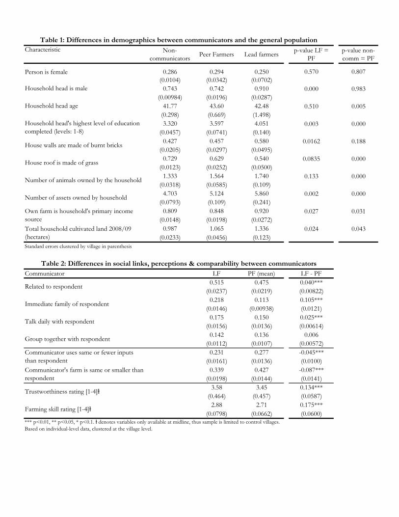
Characteristic Non-communicators

Peer Farmers Lead farmersp-value LF =

PFp-value non-comm = PF

0.286 0.294 0.250 0.570 0.807(0.0104) (0.0342) (0.0702)

0.743 0.742 0.910 0.000 0.983(0.00984) (0.0196) (0.0287)

41.77 43.60 42.48 0.510 0.005(0.298) (0.669) (1.498)3.320 3.597 4.051 0.003 0.000

(0.0457) (0.0741) (0.140)0.427 0.457 0.580 0.0162 0.188

(0.0205) (0.0297) (0.0495)0.729 0.629 0.540 0.0835 0.000

(0.0123) (0.0252) (0.0500)1.333 1.564 1.740 0.133 0.000

(0.0318) (0.0585) (0.109)4.703 5.124 5.860 0.002 0.000

(0.0793) (0.109) (0.241)0.809 0.848 0.920 0.027 0.031

(0.0148) (0.0198) (0.0272)0.987 1.065 1.336 0.024 0.043

(0.0233) (0.0456) (0.123)

Communicator LF PF (mean) LF - PF0.515 0.475 0.040***

(0.0237) (0.0219) (0.00822)0.218 0.113 0.105***

(0.0146) (0.00938) (0.0121)0.175 0.150 0.025***

(0.0156) (0.0136) (0.00614)0.142 0.136 0.006

(0.0112) (0.0107) (0.00572)0.231 0.277 -0.045***

(0.0161) (0.0136) (0.0100)0.339 0.427 -0.087***

(0.0198) (0.0144) (0.0141)3.58 3.45 0.134***

(0.464) (0.457) (0.0587)2.88 2.71 0.175***

(0.0798) (0.0662) (0.0600)

Standard errors clustered by village in parenthesis

Table 1: Differences in demographics between communicators and the general population

Person is female

Household head is male

Household head age

Household head's highest level of education completed (levels: 1-8)

House walls are made of burnt bricks

House roof is made of grass

Number of animals owned by the household

Number of assets owned by household

Own farm is household's primary income source

Total household cultivated land 2008/09 (hectares)

Communicator's farm is same or smaller than respondent

Trustworthiness rating [1-4]ⱡ

Farming skill rating [1-4]ⱡ

*** p<0.01, ** p<0.05, * p<0.1. ⱡ denotes variables only available at midline, thus sample is limited to control villages. Based on individual-level data, clustered at the village level.

Table 2: Differences in social links, perceptions & comparability between communicators

Related to respondent

Immediate family of respondent

Talk daily with respondent

Group together with respondent

Communicator uses same or fewer inputs than respondent

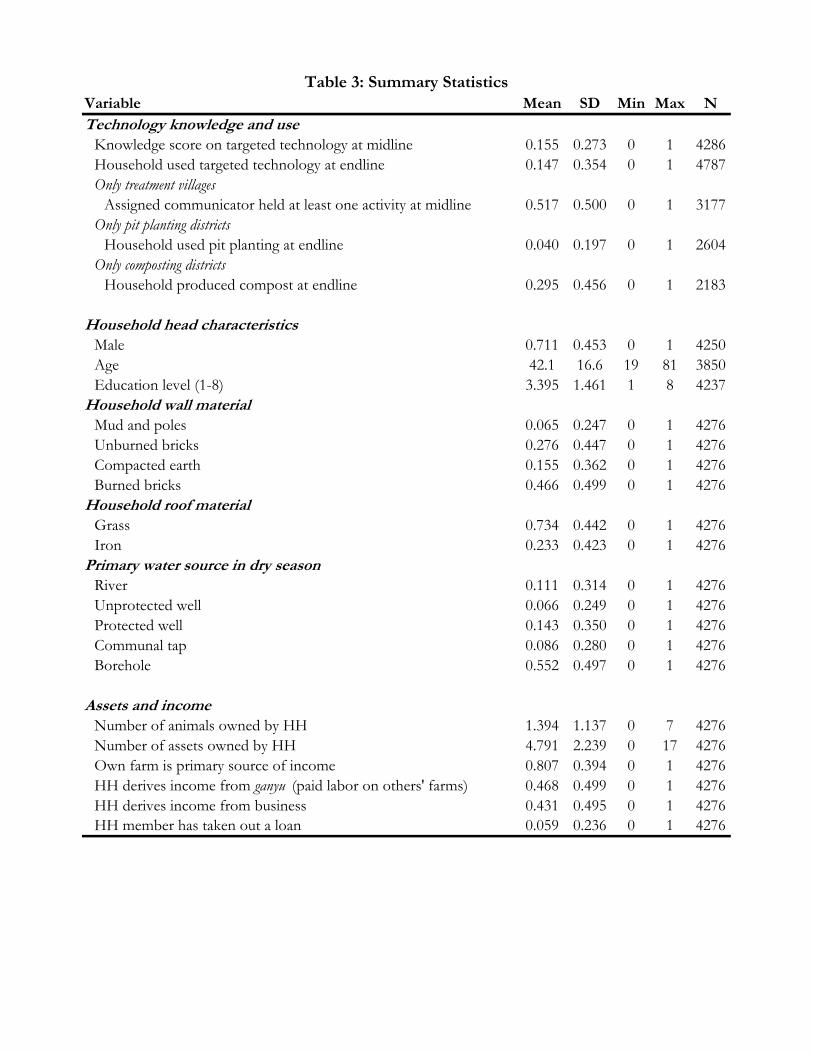
Variable Mean SD Min Max NTechnology knowledge and use

Knowledge score on targeted technology at midline 0.155 0.273 0 1 4286Household used targeted technology at endline 0.147 0.354 0 1 4787Only treatment villages

Assigned communicator held at least one activity at midline 0.517 0.500 0 1 3177Only pit planting districts

Household used pit planting at endline 0.040 0.197 0 1 2604Only composting districts

Household produced compost at endline 0.295 0.456 0 1 2183

Household head characteristicsMale 0.711 0.453 0 1 4250Age 42.1 16.6 19 81 3850Education level (1-8) 3.395 1.461 1 8 4237

Household wall materialMud and poles 0.065 0.247 0 1 4276Unburned bricks 0.276 0.447 0 1 4276Compacted earth 0.155 0.362 0 1 4276Burned bricks 0.466 0.499 0 1 4276

Household roof materialGrass 0.734 0.442 0 1 4276Iron 0.233 0.423 0 1 4276

Primary water source in dry seasonRiver 0.111 0.314 0 1 4276Unprotected well 0.066 0.249 0 1 4276Protected well 0.143 0.350 0 1 4276Communal tap 0.086 0.280 0 1 4276Borehole 0.552 0.497 0 1 4276

Assets and incomeNumber of animals owned by HH 1.394 1.137 0 7 4276Number of assets owned by HH 4.791 2.239 0 17 4276Own farm is primary source of income 0.807 0.394 0 1 4276HH derives income from ganyu (paid labor on others' farms) 0.468 0.499 0 1 4276HH derives income from business 0.431 0.495 0 1 4276HH member has taken out a loan 0.059 0.236 0 1 4276

Table 3: Summary Statistics

(1) (2) (3) (4) (5) (6) (7) (8)

0.0683 0.0703 0.0800** 0.0718** -0.211** -0.154 0.0125 -0.0480(0.0584) (0.0456) (0.0352) (0.0348) (0.102) (0.121) (0.0656) (0.0727)

0.102 0.106* 0.217*** 0.210*** 0.0929 0.128 0.404*** 0.386***(0.0774) (0.0639) (0.0529) (0.0538) (0.142) (0.127) (0.100) (0.0854)0.0356 0.0360 0.202*** 0.177*** -0.121 -0.0967 0.344*** 0.292***

(0.0419) (0.0372) (0.0466) (0.0473) (0.0838) (0.0839) (0.0974) (0.0766)

0.303*** 0.369*** -0.292*** -0.397***(0.0451) (0.0319) (0.0779) (0.0574)

0.0595 0.0647 0.0854** 0.0840** -0.0225 -0.0313 -0.101 -0.0523(0.0562) (0.0477) (0.0417) (0.0422) (0.0874) (0.0783) (0.0806) (0.0560)

District FE N Y N Y N Y N YAdditional baseline controls N Y N Y N Y N Y

Observations 605 605 571 571 327 327 424 424R-squared 0.218 0.299 0.375 0.388 0.156 0.223 0.264 0.323 p-values for Actual LF = Actual PF 0.463 0.340 0.826 0.635 0.165 0.0977 0.688 0.424 Actual LF = Shadow LF 0.745 0.658 0.0365 0.0376 0.0578 0.0580 0.00199 0.000280

Mean of Dep. Var. for Shadow PFs 0.212 0.212 0.208 0.208 0.326 0.326 0.219 0.219

p-value for incentive = non-incentiveActual LF 0.258 0.006Actual PF 0.012 0.001

Dependent variable: Communicators' own adoptionUnincentivized communicators Incentivized communicators

*** p<0.01, ** p<0.05, * p<0.1. Standard errors clustered by village in parentheses. Excluded group is shadow PF. Additional baseline controls in columns 2, 4, 6, and 8 include household head gender, education and age, household wall and roof construction materials and primary source of water in dry and wet seasons, staple food consumed by household, number of animals and assets owned by household, primary sources of farming income (own farm, others’ farm, own business), and whether anyone in the household had taken a loan in the preceding 12 months. Knowledge scores include zero scores for respondents who answered that they were not aware of the technology.

Table 4: Knowledge Retention and Adoption by Communicators

Pit planting district

Dependent variable: Communicators' Knowledge scoresUnincentivized communicators Incentivized communicators

Shadow LF

Actual LF assigned to CommunicationActual PF assigned to communication

Majority Female Communicators

(1) (2) (3) (4)

0.457*** 0.183 0.640*** 0.752***(0.0510) (0.160) (0.0607) (0.136)0.411*** 0.231 0.617*** 0.722***(0.0743) (0.165) (0.0760) (0.123)0.410*** 0.116 0.741*** 0.834***(0.0784) (0.146) (0.0794) (0.131)

-0.0949 -0.106* 0.0145 0.0467(0.0715) (0.0564) (0.0726) (0.0673)

Pit Planting Dummy Y - Y -District FE N Y N YAdditional baseline controls N Y N Y

Observations 1,716 1,430 1,528 1,334R-squared 0.471 0.534 0.611 0.654p-values for

AEDO = LF 0.526 0.472 0.760 0.661AEDO = PF 0.557 0.259 0.222 0.220LF = PF 0.995 0.0679 0.0950 0.0745

p-value for incentive = non-incentive

AEDO 0.231 0.0375LF 0.0463 0.295PF 0.0113 0.000174

Table 5: Communicator Effort to Transmit KnowledgeDependent variable: Designated communicator held at least one activityUnincentivized communicators Incentivized communicators

*** p<0.01, ** p<0.05, * p<0.1. Standard errors clustered by village in parentheses. Sample excludes control villages. Additional baselinecontrols in columns 2 and 4 include household head gender, education and age, household wall and roof construction materials and primarysource of water in dry and wet seasons, staple food consumed by household, number of animals and assets owned by household, primarysources of farming income (own farm, others’ farm, own business), and whether anyone in the household had taken a loan in the preceding12 months.

AEDO treatment

LF treatment

PF treatment

Majority Female Communicators

0.219*** 0.202*** 0.0640** 0.0674**(0.0719) (0.0539) (0.0292) (0.0267)0.0916** 0.0685** 0.0624** 0.0639**(0.0384) (0.0300) (0.0276) (0.0286)0.0266 0.0187 0.112*** 0.102***

(0.0264) (0.0258) (0.0365) (0.0357)0.169*** 0.222***(0.0299) (0.0230)-0.0305 -0.00796 0.0423 0.0491*(0.0303) (0.0192) (0.0301) (0.0285)

District FE N Y N YAdditional baseline controls N Y N YObservations 2,875 2,463 2,687 2,367R-squared 0.180 0.258 0.220 0.260p-values for

AEDO = LF 0.103 0.0255 0.957 0.908AEDO = PF 0.00963 0.00407 0.195 0.349LF = PF 0.0757 0.122 0.177 0.280

Mean of Dep. Var. for Control Villages 0.0977 0.0968 0.0977 0.0968

Mean of Dep. Var. for AEDO Villages

0.308 0.318 0.134 0.138

p-value for incentive = non-incentiveAEDO 0.0620 0.0259LF 0.932 0.778PF 0.0228 0.00929

Table 6: Knowledge after one season among target farmers Dependent variable: Knowledge scores in household survey

Unincentivized communicators Incentivized communicators

*** p<0.01, ** p<0.05, * p<0.1. Standard errors clustered by village in parentheses. Excluded group is control villages. Additional baseline controls in columns2 and 4 include household head gender, education and age, household wall and roof construction materials and primary source of water in dry and wet seasons,staple food consumed by household, number of animals and assets owned by household, primary sources of farming income (own farm, others’ farm, ownbusiness), and whether anyone in the household had taken a loan in the preceding 12 months. Dependent variable includes zero scores for respondents whoanswered that they were not aware of the technology.

AEDO treatment

LF treatment

PF treatment

Pit planting district

Majority Female Communicators

Technology

Dependent variable

Communicator incentivesNon-

incentiveIncentive

Non-incentive

IncentiveNon-

incentiveIncentive

Non-incentive

Incentive

(1) (2) (3) (4) (5) (6) (7) (8)

0.0235*** 0.0707*** 0.0958*** -0.0246 0.0908** 0.0278 0.00726 0.188*(0.00759) (0.0262) (0.0144) (0.0524) (0.0360) (0.0323) (0.0747) (0.0999)-0.00644 0.0881** 0.0339 0.0773 0.0157 0.118** -0.0541 0.181**(0.00964) (0.0401) (0.0240) (0.0572) (0.0427) (0.0502) (0.0619) (0.0710)0.0121* 0.142*** 0.0808 0.146*** 0.0875** 0.148*** -0.0757 0.298***

(0.00652) (0.0286) (0.0722) (0.0483) (0.0377) (0.0435) (0.0601) (0.0722)

0.0245*** 0.0246 0.0407 0.0552 -0.0215 -0.0750(0.00735) (0.0225) (0.0300) (0.0363) (0.0479) (0.0687)

District FE Y Y Y Y Y Y Y Y

Observations 1,792 1,078 260 519 1,792 1,686 1,456 1,091

p-values forAEDO = LF p-value 0.00652 0.657 0.0000 0.0877 0.0638 0.0703 0.509 0.942AEDO = PF p-value 0.148 0.0106 0.561 0.00588 0.935 0.00289 0.353 0.297LF = PF p-value 0.0626 0.0577 0.207 0.783 0.0864 0.560 0.718 0.112

Mean of Dep. Var. for Control Villages 0.00782 0.0127 0 0 0.0821 0.0821 0.241 0.241

Mean of Dep. Var. for AEDO Villages 0.052 0.033 0.0833 0 0.214 0.108 0.198 0.443

p-value for incentive = non-incentiveAEDO 0.825 0.376 0.0114 0.132LF 0.00719 0.103 0.0999 0.0265PF 0.0187 0.787 0.458 0.0000

*** p<0.01, ** p<0.05, * p<0.1. Estimates in columns (3) and (4) are OLS coefficients; all other columns report average marginal effects from probit regression. Standard errors clusteredby village in parentheses. Excluded group is control villages. Columns 3 and 4 use the random subsamples of households in PP villages for which direct observation was conducted(sample sizes are limited because it was expensive to do the direct observation. We allocated a larger sample size to incentive villages in order to validate the self-report data on the basis ofwhich incentives were awarded).

AEDO treatment

LF treatment

PF treatment

Table 7: Adoption after two seasons among Target FarmersPit Planting Composting

Used on at least one household plot in 2010/11

Plan to use next yearHousehold produced at

least compost heap

Directly observed usage on at least one plot in

2010/11

Majority Female Communicators

(1) (2) (3) (4)

Dependent variable

Sample

Incentives? Non-incentive Incentive Non-incentive Incentive

PF village 0.0138 0.145** -0.00459 0.151**(0.0496) (0.0604) (0.0533) (0.0726)

Communicators per HH -0.501 -0.361 -0.330 -6.284*(0.631) (0.874) (2.349) (3.289)

Pit planting district -0.198*** -0.292*** -0.240** -0.276***(0.0422) (0.0348) (0.0935) (0.0394)-0.00616 -0.104*** 0.0388 -0.108*(0.0365) (0.0402) (0.0590) (0.0650)

Observations 1,742 1,311 649 493Mean of Dependent Var in LF 0.113 0.193 0.117 0.147

common support min 0.0588

*** p<0.01, ** p<0.05, * p<0.1

Table 8: Communicators per HH

Robust standard errors clustered by village in parentheses. Cols 1-4 estimated via OLS; cols 5-8 estimated via probit, with average marginal effects shown. Common support sample (cols 3-4 and 7-8) is limited to villages where communicators per capita is between the minimum value for PF villages and the maximum value for LF villages.

Household adopted target technology in 2010/11 season

All LF and PF villages Common support

Majority Female Communicators

Alternative hypothesis:

LF villages with <=65

hh

PF vill. with > 65 hhs

PF vill. with > 100 hs

PFs related to one another

PFs in group with one another

PFs talk daily with one another

(1) (2) (3) (4) (5) (6)Average marginal effect of

0.122* 0.239*** 0.277***(0.0684) (0.0445) (0.0611)

0.249*** 0.206*** 0.186***(0.0396) (0.0405) (0.0428)0.219*** 0.253*** 0.269***(0.0672) (0.0354) (0.0468)

p-value for incentive @ 25th pct = incentive

@ 75th pct 0.621 0.165 0.0855

0.00648 -0.0399 -0.00640

(0.0659) (0.0496) (0.0678)

Mean of Dep Var in LF Non-incentive Villages

0.129

Mean of Dep Var in PF Non-incentive Villages

0.106 0.0828 0.0831 0.0831 0.0831

Observations 781 512 332 1566 1566 1566

*** p<0.01, ** p<0.05, * p<0.1. Estimates shown are average marginal effects from probit regression: adopt = f(β incentive+λ pitplanting+γ majority female comms) . Sample includes all non-communicator households. Standard errors clustered by village in parentheses.

Incentive village @ 25th percentile of PF links

Incentive village

Table 9: Testing Alternative Hypotheses Controlling for Communicator Gender

Incentive village @ 75th percentile of PF links

Jointness of incentivesDependent variable: Household adopted target technology in 2010/11 season

Non-linearity of incentives

Majority Female Communicators Included as control

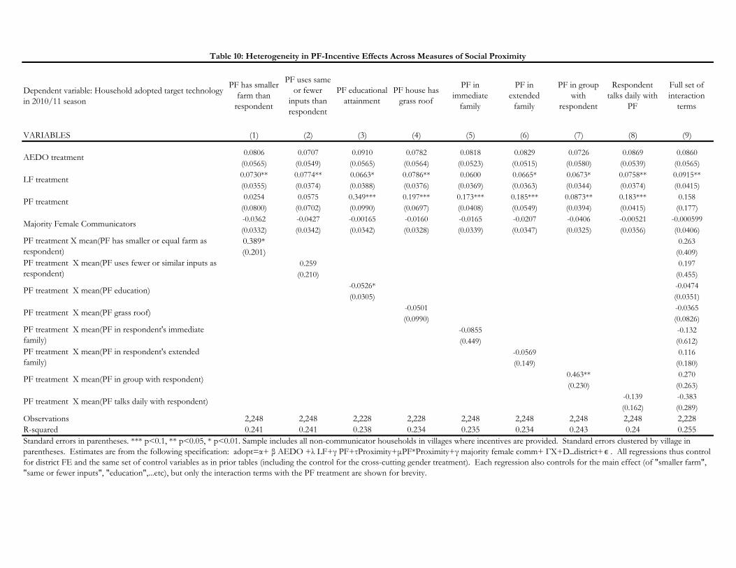
Dependent variable: Household adopted target technology in 2010/11 season

VARIABLES (1) (2) (3) (4) (5) (6) (7) (8) (9)

0.0806 0.0707 0.0910 0.0782 0.0818 0.0829 0.0726 0.0869 0.0860(0.0565) (0.0549) (0.0565) (0.0564) (0.0523) (0.0515) (0.0580) (0.0539) (0.0565)0.0730** 0.0774** 0.0663* 0.0786** 0.0600 0.0665* 0.0673* 0.0758** 0.0915**(0.0355) (0.0374) (0.0388) (0.0376) (0.0369) (0.0363) (0.0344) (0.0374) (0.0415)0.0254 0.0575 0.349*** 0.197*** 0.173*** 0.185*** 0.0873** 0.183*** 0.158

(0.0800) (0.0702) (0.0990) (0.0697) (0.0408) (0.0549) (0.0394) (0.0415) (0.177)-0.0362 -0.0427 -0.00165 -0.0160 -0.0165 -0.0207 -0.0406 -0.00521 -0.000599(0.0332) (0.0342) (0.0342) (0.0328) (0.0339) (0.0347) (0.0325) (0.0356) (0.0406)0.389* 0.263(0.201) (0.409)

0.259 0.197(0.210) (0.455)

-0.0526* -0.0474(0.0305) (0.0351)

-0.0501 -0.0365(0.0990) (0.0826)

-0.0855 -0.132(0.449) (0.612)

-0.0569 0.116(0.149) (0.180)

0.463** 0.270(0.230) (0.263)

-0.139 -0.383(0.162) (0.289)

Observations 2,248 2,248 2,228 2,228 2,248 2,248 2,248 2,248 2,228R-squared 0.241 0.241 0.238 0.234 0.235 0.234 0.243 0.24 0.255

Majority Female Communicators

Table 10: Heterogeneity in PF-Incentive Effects Across Measures of Social Proximity

LF treatment

PF treatment

AEDO treatment

PF in immediate

family

PF in extended

family

PF in group with

respondent

Respondent talks daily with

PF

PF has smaller farm than

respondent

PF uses same or fewer

inputs than respondent

PF educational attainment

PF house has grass roof

Full set of interaction

terms

Standard errors in parentheses. *** p<0.1, ** p<0.05, * p<0.01. Sample includes all non-communicator households in villages where incentives are provided. Standard errors clustered by village in parentheses. Estimates are from the following specification: adopt=α+ β AEDO +λ LF+γ PF+τProximity+μPF*Proximity+γ majority female comm+ ΓX+D_district+ϵ . All regressions thus control for district FE and the same set of control variables as in prior tables (including the control for the cross-cutting gender treatment). Each regression also controls for the main effect (of "smaller farm", "same or fewer inputs", "education",...etc), but only the interaction terms with the PF treatment are shown for brevity.

PF treatment X mean(PF has smaller or equal farm as respondent)PF treatment X mean(PF uses fewer or similar inputs as respondent)

PF treatment X mean(PF education)

PF treatment X mean(PF grass roof)

PF treatment X mean(PF in respondent's immediate family)PF treatment X mean(PF in respondent's extended family)

PF treatment X mean(PF in group with respondent)

PF treatment X mean(PF talks daily with respondent)

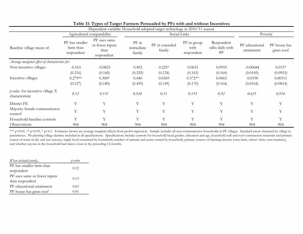
Baseline village mean of: PF in

immediate family

Average marginal effect of characteristic for: -0.163 -0.0823 0.492 0.225* 0.0651 0.0955 -0.00684 0.0157(0.216) (0.160) (0.329) (0.124) (0.163) (0.164) (0.0169) (0.0953)0.279** 0.300* 0.440 0.0369 0.372** 0.0663 -0.0190 0.00311(0.127) (0.180) (0.459) (0.149) (0.170) (0.164) (0.0164) (0.0814)

p-value for incentive village X characteristic 0.12 0.131 0.924 0.31 0.153 0.92 0.625 0.914

District FE Y Y Y Y Y Y Y YMajority female communicator control Y Y Y Y Y Y Y Y

Household baseline controls Y Y Y Y Y Y Y YObservations 904 904 904 904 904 904 904 904

When included jointly... p-valuePF has smaller farm than respondent

0.12

PF uses same or fewer inputs than respondent

0.13

PF educational attainment 0.63PF house has grass roof 0.91

Social LinksDependent variable: Household adopted target technology in 2010/11 season

Table 11: Types of Target Farmers Persuaded by PFs with and without Incentives

*** p<0.01, ** p<0.05, * p<0.1. Estimates shown are average marginal effects from probit regression. Sample includes all non-communicator households in PF villages. Standard errors clustered by village in parentheses. Pit planting village dummy included in all specifications. Specifications include controls for household head gender, education and age, household wall and roof construction materials and primary source of water in dry and wet seasons, staple food consumed by household, number of animals and assets owned by household, primary sources of farming income (own farm, others’ farm, own business), and whether anyone in the household had taken a loan in the preceding 12 months.

Non-incentive villages

Incentive villages

Agricultural comparability Poverty

PF has smaller farm than

respondent

PF uses same or fewer inputs

than respondent

PF educational attainment

PF house has grass roof

PF in group with

respondent

Respondent talks daily with

PF

PF in extended family

Appendix Figure A1

Panel A: PF/LF Communicator Arms with Cross‐Cutting Gender Assignment

Incentive Non-incentive Incentive Non-incentiveFemale-assigned 13 12 12 11Non-female-assigned 12 13 11 11

Incentive Non-incentive Incentive Non-incentiveFemale-assigned 0.55 0.67 0.49 0.46Non-female-assigned 0 0 0.3 0.33Overall 0.29 0.32 0.4 0.4

Incentive Non-incentive Incentive Non-incentiveFemale-assigned 0.55 0.67 0.46 0.64Non-female-assigned 0 0 0.18 0.18Overall 0.29 0.32 0.33 0.41

Panel B. Gender assignment in LF and PF arms: Number of villages in each cellLF PF

Panel D. Gender compliance in LF and PF arms: Share of villages with majority female communicators

LF PF

Panel C. Control for Gender compliance: Proportion of communicators in village that are female

LF PF

Lead farmer (LF)

Peer farmer

(PF)

Incentive No Incentive Incentive No Incentive

Female-reserved

[13 vill]

Non-reserved

[12 vill]

Female-reserved

[12 vill]

Non-reserved

[13 vill]

Female-reserved

[12 vill]

Non-reserved

[11 vill]

Female-reserved

[11 vill]

Non-reserved

[11 vill]

Appendices for BenYishay and Mobarak, REStud MS 19500 “Social Learning and Incentives for Experimentation and Communication”

 

Appendix A1: Training Protocol

In August 2009, the Ministry of Agriculture and Food Security (MoAFS) conducted trainings for all the Agricultural Extension Development Officers (AEDOs) and Agricultural Extension Development Coordinators (AEDCs; supervisors of AEDOs) covering the 120 treatment sections. The Department of Agricultural Extension Services (DAES) coordinated the trainings, which were jointly facilitated with the Departments of Agricultural Research Services (DARS) and Land Resources Conservation (DLRC). Four training sessions were conducted nationally, at the MoAFS Residential Training Centers in Lunzu, Thyolo and Mzimba. Staff in areas targeted for the conservation farming intervention were training separately from those in areas targeted for the nutrient management intervention. AEDOs and AEDCs were trained only in the technology relevant to their work area. Trainings lasted for three days, and covered the following:

Day 1 ◦ Overview of the research study, focusing on motivation and research questions ◦ Review of the concept of lead farmer. DAES had promoted working with lead farmers since

2006, so some (but not all) of the AEDOs were familiar with the role of a lead farmer and how to select a lead farmer.

◦ Introduction to the concept of peer farmer. As this concept was developed by DAES and the study research team, this was a new topic for all the AEDOs.

Day 2 ◦ Classroom explanation of conservation farming / nutrient management technologies, with

specific discussion of pit planting/Chinese composting. ◦ Hands-on training in pit planting /Chinese composting using the demonstration plots at the

Training Centres. Day 3

◦ Visits to farmers who had adopted pit planting / Chinese composting to discuss the experience ◦ Explanation to each AEDO of the specific village assignment, whether he/she was to work with

a lead or peer farmer in the village, and whether there were any gender requirements for the extension partner.

Training of Extension Partners (Lead and Peer Farmers)

At the training, AEDOs were assigned to select lead and peer farmers in the target villages by the end of August. Although AEDOs were told to work primarily with either a lead or peer farmer (or neither, depending on assigned communication strategy), they were asked to identify one lead farmer and five peer farmers in all villages in order for data collection about social networks to be complete and unbiased. In control villages, “shadow” lead and peer farmers (six representatives of different social networks in the village) were identified through village focus groups facilitated by the field supervisors of the data collection teams, for accurate comparison of social networks. As soon as the lead and peer farmers were identified, their names were reported back to the District office of the Ministry of Agriculture and Food Security, to ensure that those households were all sampled in the baseline survey.

The AEDOs assigned to work with either lead farmers or peer farmers trained those individuals in their home villages during the month of September. Typically, the training lasted for half of a day and involved an explanation of the new technology as well as a practical demonstration. The AEDOs then made follow-ups with the lead and peer farmers over the next few months, often assisting them to set up demonstration plots on their own fields.

 

Appendix A2: Technical Specifications of Pit Planting and Nutrient Management

Specifications for Pit Planting

Pit planting is a conservation farming technology that increases a soil’s capacity for storing water while at the same time allowing for minimum soil disturbance. This is because when planting pits are excavated in a field, they may be used for at least two seasons before farmers have to reshape the pits. Planting pits enable farmers to use small quantities of water and manure very efficiently, and are cost and time efficient (although labor to construct the pits can be a constraint). Pits are ideal in areas where rainfall is limited.

The following are the guidelines for pit planting that the project will employ. These guidelines were developed by the MoAFS Department of Land Resources Management.

Step 1: Site Selection

Identify a plot with relatively moderate slopes. If possible the site should be secure from livestock to protect the crop residues.

Step 2: Land Preparation

Mark out the pit position using a rope, and excavate the pits following the recommended dimensions (as shown in the table below). These should be dug along the contour. The soil should be placed on the down slope side. Stones may be placed on the upslope side of the pit to help control run off, but this is optional. If available, crop residues from the previous harvest should be retained in the field so there is maximum ground cover.

Pit dimension and spacing:

Spacing between pits 70cm Spacing between rows 75cm Depth 15cm Length 30cm Width 15cm

At this spacing, there will be 15,850 pits per hectare (158 pits per 0.1ha). Where rainfall is limited, pits can be made deeper and wider to make maximum use of rainwater.

Step 3: Planting, Manure and Fertilizer Application

The pit can be planted to maize crop at the spacing below:

Crop Seeds/pit Plants/ha Maize 2 56,000

It is recommended that farmers apply 2 handfuls of manure in each pit. Two weeks before rainfall, apply manure and cover the pit with earth. If basal fertilizer is available, it can also be applied at the same time. When manure has been applied, the pits should be covered with soil. A shallow depression should still remain on top.

If top dressing is available, it should be applied when the maize is kneed high. In some areas, it may be after 21 days. Use the local area recommendations to calculate the right amount to be applied (refer to the Guide to Agricultural Production in Malawi).

 

Step 4: Weed Control and Pest Management

The pits must be kept free of weeds at all times. Weed as soon as the weeds appear and just before harvesting. This will reduce the amount of weeds in the following season. Use of herbicides to control weeds is optional.

Step 5: Harvesting

Remove the crop. Cut plants at base, leaving stems and leaves on the soil. The roots should not be uprooted; they should be left to decompose within the pit.

Increasing the Efficiency of the Pits

It is important to realize that the use of these pits alone will not produce the highest yields. For best results:

Always incorporate crop residues, leaving a minimum of 30% of crop residue on the field. Apply manure generously. Protect crops from weeds, pests, and diseases. Always plant with the first productive rains. Grow crops in rotation; at least 30% of the cropped land should be planted to legumes.

Guidelines for Nutrient Management

Below are the guidelines to the nutrient management strategy the project will employ. These guidelines were developed by the MoAFS Department of Agricultural Research.

Step 1: Materials for Making Compost

The following materials are appropriate for making compost:

Leguminous crop residues (Ground-nuts and Soyabean) Fresh leaves of leguminous trees Chopped maize stover (about 6 inches long) Animal or Chicken manure (Optional)

Mix three parts of leguminous biomass (crop residues and/or fresh leaves) to two parts maize stover

Step 2: Composting method

Put a layer of legume crop residue followed by a layer of stover then a layer of green leaves of legume tree repeat making the layers until the heap is 120 cm high. After constructing a set of three layers add 5 liters of water to moisten the materials.

After constructing the heap smear the wet earth around the heap covering the biomass. The materials should be kept moist throughout the composting period. After 60 days the manure is ready, remove the manure and keep them under shade

Step 3: Application method

Apply the manure at least two weeks before planting. Apply 3 kg of manure applied per 10 m ridge. Split open the ridge about 4 cm deep, spread the manure on the open ridge then bury the manure thus reconstituting the ridge.

Step 4: Planting

 

At the rain onset plant maize, one maize seed per planting hole on the ridge at a distance of 25 cm between planting holes.

Step 5: Use of Inorganic Fertilizer (optional, depends on availability)

Use 23:21:0+4S for basal dressing. Apply fertilizer as dollop; make a hole about 3 cm deep between the maize planting hills.

Apply 60 kg N/ha of 23:21:0+4S at a rate 2g per hole (cups to be calibrated to measure 2 g fertilizer).

Apply the inorganic fertilizer one (1) week after maize germination

Knowledge Questions Administered in Household Surveys

 

 

Pit Planting

Knowledge Question Correct answer (acceptable range)

How far apart should the planting pits be? 70 cm (52.5 cm – 87.5 cm) How deep should planting pits be? 20 cm (15 cm – 25 cm)How wide should planting pits be? 30 cm (22.5 cm – 37.5 cm) How long should planting pits be? 30 cm (22.5 cm – 37.5 cm) How many maize seeds should be planted in each pit?

4

Should manure be applied? Yes How much manure should be applied? 2 double handfuls After harvest what should be done with the stovers? Maize plants cut off at base, leave roots to decompose

in pit, stems and leaves used to cover the soil.

Chinese Compost Knowledge Question Correct answer (acceptable range) What materials should be used for Chinese composting?

leguminous crop residues, fresh leaves of leguminous trees, maize stoves, chicken or livestock manure

How much time should Chinese compost be let mature?

60 days (48 – 72 days)

How should Chinese compost be kept while it is maturing?

in a covered heap

Should it be kept in the sun or the shade? Shade Should it be kept moist or dry? Moist When should Chinese compost be applied to the field? at least 2 weeks before planting

(1) (2) (3) (4) (5) (6) (7) (8) (9) (10) (11)

Household used pit

planting on at least one plot in 2008/9 ¹

Household used any

composting in 2008/9 ²

Household head is male

Household head age

Household head's

highest level of education completed (levels: 1-8)

House walls are made of burnt bricks

House roof is made of grass

Number of animals

owned by the household

Number of assets owned by household

Own farm is household's

primary income source

Total household cultivated

land 2008/09 (hectares)

AEDO inc = AEDO no inc 0.664 0.350 0.639 0.704 0.271 0.176 0.505 0.382 0.448 0.943 0.514

AEDO inc = LF inc 0.602 0.222 0.511 0.458 0.358 0.951 0.844 0.315 0.400 0.244 0.452

AEDO inc = LF no inc 0.405 0.172 0.966 0.663 0.242 0.003 0.306 0.992 0.439 0.878 0.956

AEDO inc = PF inc 0.803 0.279 0.394 0.597 0.915 0.801 0.777 0.369 0.597 0.943 0.163

AEDO inc = PF no inc 0.664 0.187 0.897 0.885 0.376 0.805 0.740 0.931 0.922 0.157 0.600

AEDO inc = Cont 0.742 0.911 0.849 0.806 0.115 0.099 0.304 0.982 0.937 0.817 0.828

AEDO no inc = LF inc 0.366 0.207 0.146 0.784 0.660 0.160 0.369 0.905 0.053 0.079 0.874

AEDO no inc = LF no inc 0.745 0.928 0.575 0.993 0.856 0.501 0.951 0.334 0.069 0.775 0.410

AEDO no inc = PF inc 0.877 0.229 0.689 0.331 0.207 0.202 0.333 0.972 0.127 0.998 0.350

AEDO no inc = PF no inc 0.958 0.271 0.638 0.532 0.707 0.144 0.604 0.263 0.263 0.025 0.939

AEDO no inc = Cont 0.445 0.351 0.645 0.440 0.936 0.756 0.966 0.277 0.338 0.770 0.556

LF inc = LF no inc 0.173 0.136 0.337 0.718 0.705 0.002 0.083 0.262 0.922 0.244 0.364

LF inc = PF inc 0.492 0.589 0.022 0.074 0.236 0.741 0.906 0.934 0.677 0.053 0.442

LF inc = PF no inc 0.323 0.604 0.257 0.216 0.953 0.842 0.457 0.218 0.271 0.001 0.837

LF inc = Cont 0.754 0.368 0.159 0.113 0.368 0.073 0.067 0.211 0.139 0.042 0.484

LF no inc = PF inc 0.603 0.135 0.265 0.202 0.152 0.001 0.063 0.310 0.742 0.763 0.097

LF no inc = PF no inc 0.675 0.130 0.907 0.444 0.800 0.005 0.320 0.932 0.312 0.066 0.534

LF no inc = Cont 0.259 0.278 0.827 0.312 0.687 0.113 0.968 0.969 0.172 0.637 0.736

PF inc = PF no inc 0.905 0.917 0.316 0.601 0.298 0.633 0.399 0.268 0.538 0.024 0.370

PF inc = Cont 0.598 0.547 0.265 0.609 0.044 0.092 0.055 0.267 0.371 0.767 0.136

PF no inc = Cont 0.398 0.522 0.934 0.893 0.531 0.096 0.297 0.892 0.784 0.041 0.683

Appendix A3: Balance Testsp-value for ...

¹ Sample limited to pit planting districts; ² Sample limited to composting districts; Sample in all other rows includes all districts. Gray shading denotes p<0.05. Standard errors clustered by village in parentheses. All tests based on comparisons of means controlling for district fixed effects.

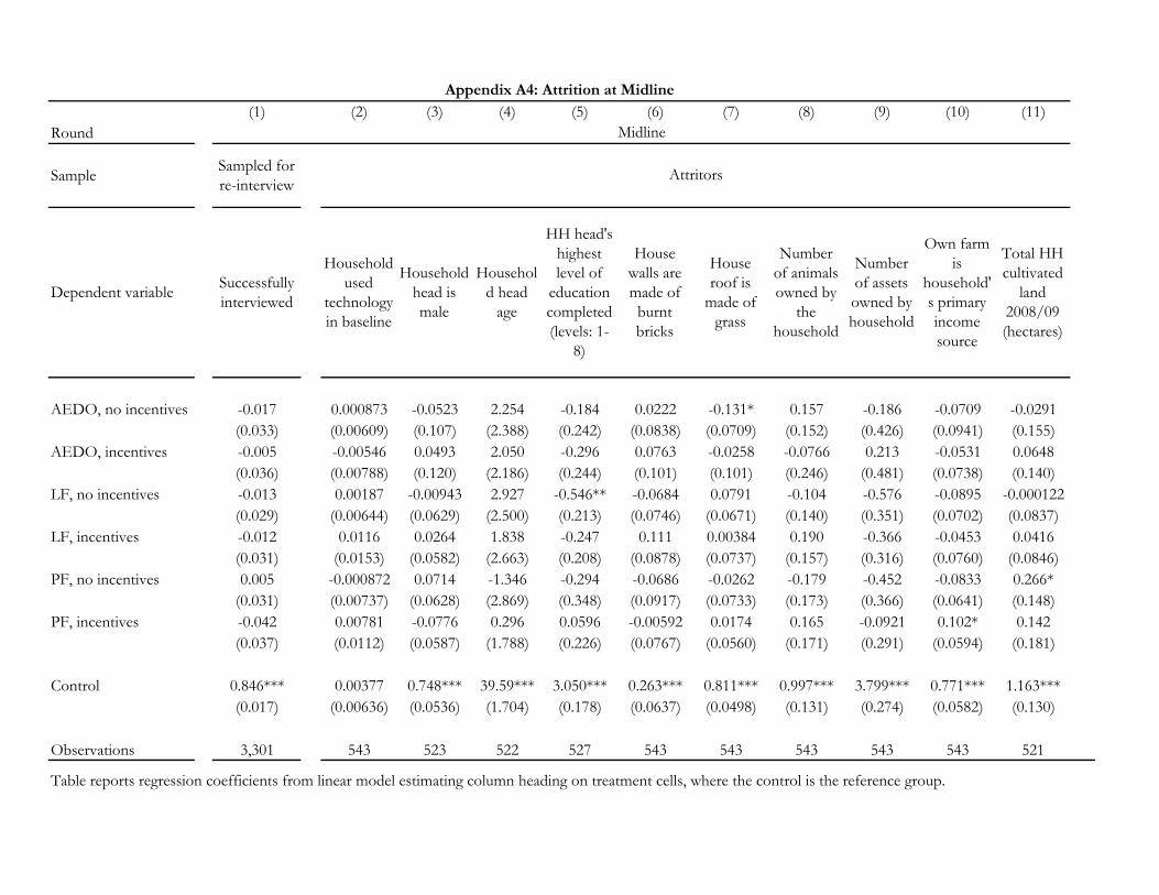
(1) (2) (3) (4) (5) (6) (7) (8) (9) (10) (11)Round

SampleSampled for re-interview

Dependent variableSuccessfully interviewed

Household used

technology in baseline

Household head is male

Household head

age

HH head's highest level of

education completed (levels: 1-

8)

House walls are made of

burnt bricks

House roof is

made of grass

Number of animals owned by

the household

Number of assets owned by household

Own farm is

household's primary income source

Total HH cultivated

land 2008/09 (hectares)

AEDO, no incentives -0.017 0.000873 -0.0523 2.254 -0.184 0.0222 -0.131* 0.157 -0.186 -0.0709 -0.0291(0.033) (0.00609) (0.107) (2.388) (0.242) (0.0838) (0.0709) (0.152) (0.426) (0.0941) (0.155)

AEDO, incentives -0.005 -0.00546 0.0493 2.050 -0.296 0.0763 -0.0258 -0.0766 0.213 -0.0531 0.0648(0.036) (0.00788) (0.120) (2.186) (0.244) (0.101) (0.101) (0.246) (0.481) (0.0738) (0.140)

LF, no incentives -0.013 0.00187 -0.00943 2.927 -0.546** -0.0684 0.0791 -0.104 -0.576 -0.0895 -0.000122(0.029) (0.00644) (0.0629) (2.500) (0.213) (0.0746) (0.0671) (0.140) (0.351) (0.0702) (0.0837)

LF, incentives -0.012 0.0116 0.0264 1.838 -0.247 0.111 0.00384 0.190 -0.366 -0.0453 0.0416(0.031) (0.0153) (0.0582) (2.663) (0.208) (0.0878) (0.0737) (0.157) (0.316) (0.0760) (0.0846)

PF, no incentives 0.005 -0.000872 0.0714 -1.346 -0.294 -0.0686 -0.0262 -0.179 -0.452 -0.0833 0.266*(0.031) (0.00737) (0.0628) (2.869) (0.348) (0.0917) (0.0733) (0.173) (0.366) (0.0641) (0.148)

PF, incentives -0.042 0.00781 -0.0776 0.296 0.0596 -0.00592 0.0174 0.165 -0.0921 0.102* 0.142(0.037) (0.0112) (0.0587) (1.788) (0.226) (0.0767) (0.0560) (0.171) (0.291) (0.0594) (0.181)

Control 0.846*** 0.00377 0.748*** 39.59*** 3.050*** 0.263*** 0.811*** 0.997*** 3.799*** 0.771*** 1.163***(0.017) (0.00636) (0.0536) (1.704) (0.178) (0.0637) (0.0498) (0.131) (0.274) (0.0582) (0.130)

Observations 3,301 543 523 522 527 543 543 543 543 543 521

Table reports regression coefficients from linear model estimating column heading on treatment cells, where the control is the reference group.

Appendix A4: Attrition at Midline

Midline

Attritors

Round

Sample

Dependent variable

AEDO, no incentives

AEDO, incentives

LF, no incentives

LF, incentives

PF, no incentives

PF, incentives

Control

Observations

Table reports regression

(12) (13) (14) (15) (16) (17) (18) (19) (20) (21) (22)

Sampled for re-

interview

Successfully

interviewed

Household used

technology in baseline

Household head is male

Household head age

HH head's highest level of

education completed (levels: 1-

8)

House walls are made of

burnt bricks

House roof is

made of grass

Number of animals owned by

the household

Number of assets owned by household

Own farm is

household's primary income source

Total HH cultivated

land 2008/09 (hectares)

0.109 -0.00163 0.0123 -1.977 -0.00760 0.0176 0.0342 0.0987 0.317 -0.0625 0.139(0.0689) (0.00137) (0.0743) (2.159) (0.164) (0.0874) (0.0840) (0.157) (0.273) (0.0849) (0.159)0.131** 3.82E-05 0.0742 0.448 0.157 -0.0144 -0.0162 -0.201 0.121 -0.0971 0.295**(0.0525) (0.00142) (0.0616) (3.163) (0.236) (0.103) (0.0751) (0.157) (0.443) (0.0646) (0.145)0.0306 -0.00224 -0.0555 2.167 0.0996 -0.0281 0.0487 -0.0669 -0.112 -0.121* 0.0948

(0.0621) (0.00172) (0.0573) (2.223) (0.138) (0.0597) (0.0517) (0.133) (0.260) (0.0617) (0.0873)0.111** -0.00275 -0.0492 3.488 -0.0147 0.136* -0.0429 0.0214 -0.111 -0.0334 0.0278(0.0487) (0.00204) (0.0495) (2.128) (0.149) (0.0690) (0.0560) (0.148) (0.312) (0.0661) (0.0860)0.114** -0.00198 0.0463 -2.076 -0.0254 -0.00381 0.0721 -0.216* -0.288 -0.0727 0.295*(0.0521) (0.00170) (0.0437) (1.756) (0.146) (0.0640) (0.0586) (0.119) (0.317) (0.0568) (0.166)0.131*** 0.00670 -0.0234 -0.687 -0.168 -0.0684 0.108* -0.0406 -0.00860 0.0135 -0.0138(0.0496) (0.00750) (0.0551) (1.612) (0.180) (0.0714) (0.0560) (0.123) (0.295) (0.0513) (0.0899)

0.652*** 0.00496 0.783*** 40.10*** 3.166*** 0.328*** 0.762*** 1.197*** 3.863*** 0.860*** 0.993***(0.0437) (0.00372) (0.0531) (1.725) (0.156) (0.0579) (0.0468) (0.119) (0.272) (0.0539) (0.106)

3,711 1,023 1,023 967 1,015 1,023 1,023 1,023 1,023 1,023 1,001

Appendix A4 (continued): Attrition at Endline

Endline

Attritors

Characteristic Actual Shadow p-value Actual Shadow p-value

0.913 0.935 0.68 0.756 0.762 0.91(0.0449) (0.0273) (0.0434) (0.0310)

40 41.33 0.75 41.07 43.85 0.23(3.381) (2.436) (2.089) (0.929)

4.348 4.311 0.92 3.967 3.745 0.51

(0.159) (0.338) (0.320) (0.0979)

0.543 0.673 0.37 0.453 0.575 0.21(0.113) (0.0900) (0.0870) (0.0449)0.547 0.560 0.84 0.630 0.664 0.81

(0.0813) (0.0400) (0.107) (0.0815)1.761 1.785 0.94 1.762 1.640 0.57

(0.167) (0.263) (0.189) (0.0985)5.457 5.879 0.56 5.287 5.564 0.43

(0.451) (0.562) (0.253) (0.239)0.935 0.888 0.57 0.729 0.873 0.19

(0.0387) (0.0727) (0.107) (0.0218)1.384 1.316 0.77 0.929 1.125 0.04

(0.166) (0.160) (0.0830) (0.0475)

Household head's highest level of education completed (levels: 1-8)

Appendix A5: Differences in demographics between actual and shadow communicators

LFs PFs

Household head is male

Household head age

Standard errors clustered by village in parenthesis

House walls are made of burnt bricks

House roof is made of grass

Number of animals owned by the household

Number of assets owned by household

Own farm is household's primary income source

Total household cultivated land 2008/09 (hectares)

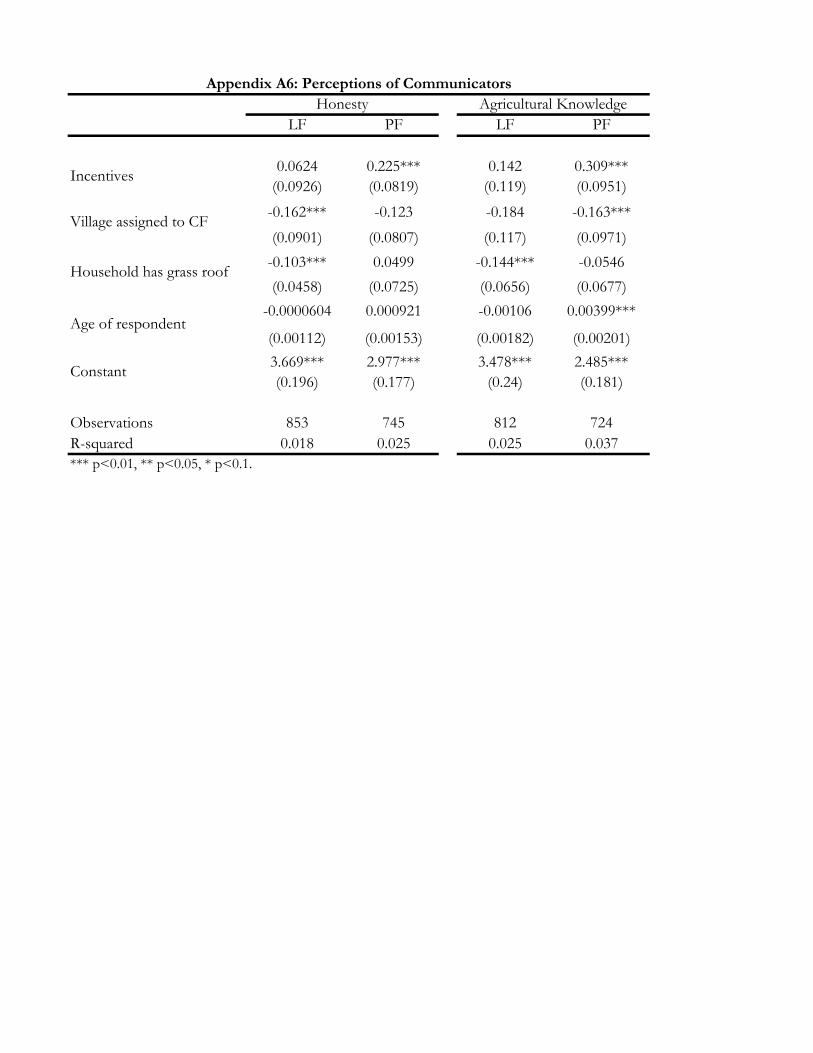
0.0624 0.225*** 0.142 0.309***(0.0926) (0.0819) (0.119) (0.0951)

-0.162*** -0.123 -0.184 -0.163***

(0.0901) (0.0807) (0.117) (0.0971)

-0.103*** 0.0499 -0.144*** -0.0546

(0.0458) (0.0725) (0.0656) (0.0677)

-0.0000604 0.000921 -0.00106 0.00399***

(0.00112) (0.00153) (0.00182) (0.00201)

3.669*** 2.977*** 3.478*** 2.485***(0.196) (0.177) (0.24) (0.181)

Observations 853 745 812 724R-squared 0.018 0.025 0.025 0.037*** p<0.01, ** p<0.05, * p<0.1.

Appendix A6: Perceptions of CommunicatorsHonesty Agricultural Knowledge

LF PF LF PF

Constant

Incentives

Village assigned to CF

Household has grass roof

Age of respondent

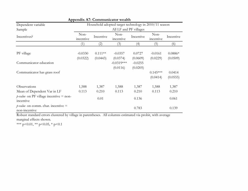
Dependent variableSample

Incentives?Non-

incentiveIncentive

Non-incentive

IncentiveNon-

incentiveIncentive

(1) (2) (3) (4) (5) (6)

PF village -0.0330 0.111** -0.0357 0.0727 -0.0161 0.0886*(0.0322) (0.0443) (0.0374) (0.0609) (0.0229) (0.0509)

Communicator education -0.0319*** -0.0255(0.0116) (0.0205)

Communicator has grass roof 0.145*** 0.0414(0.0414) (0.0555)

Observations 1,588 1,387 1,588 1,387 1,588 1,387Mean of Dependent Var in LF 0.113 0.210 0.113 0.210 0.113 0.210p-value on PF village incentive = non-incentive

0.01 0.136 0.061

p-value on comm. char. incentive = non-incentive

0.783 0.139

*** p<0.01, ** p<0.05, * p<0.1

Appendix A7: Communicator wealthHousehold adopted target technology in 2010/11 season

All LF and PF villages

Robust standard errors clustered by village in parentheses. All columns estimated via probit, with average marginal effects shown.

Technology Estimation ITT ITT IV ITT ITT IV

(1) (2) (3) (4) (5) (6)

298.1*** 178.8*** 66.11 38.18

(46.81) (65.99) (113.5) (118.3)

0.107*** 0.118 0.0633*** 0.0658

(0.0297) (0.0695) (0.0366) (0.0385)

5,020

(6,646)

143.1

(438.5)

Observations 425 358 358 532 432 432R-squared 0.306 0.306 0.145 0.169Mean baseline yieldImplied impact over baseline 17.8% 10.7% 299.3% 7.4% 3.4% 2.0%

Baseline maize yield (winsorized at 95%)

Appendix A8: Yields after two years in PF villagesDependent variable: Household maize yield in 2010/11 season

(winsorized at 95%)Pit Planting Composting

Incentive villages

HH used pit planting on any maize plot for the 2010/11 season

HH produced any compost during the 2010/11 rainy season

1678 1945

*** p<0.01, ** p<0.05, * p<0.1. Standard errors clustered by village in parentheses. Sample is limited to PF villages. Columns 1, 2, 4, and 5 show results from OLS estimation. Columns 3 and 6 show instrumental variable regressions, where incentive eligibility instruments for technology adoption.

ITT IV ITT IV ITT IV ITT IV ITT IV ITT IV  (1) (2) (3) (4) (5) (6) (7) (8) (9) (10) (11) (12)

0.112*** 0.150*** 0.170*** 0.0773 0.0385 0.0720(0.0469) (0.0331) (0.0480) (0.0842) (0.0509) (0.0513)

1.698 1.887 1.874 0.988 0.560 0.977(1.225) (1.357) (1.169) (0.615) (0.821) (0.953)

District FEs? Y Y Y Y Y Y Y Y Y Y Y YRegression Probit 2SLS Probit 2SLS Probit 2SLS Probit 2SLS Probit 2SLS Probit 2SLSObservations 765 765 765 765 765 765 765 765 765 765 765 765Mean of Dep. Var. In Non-incentive PF Villages

Appendix A9: Input Use and Pit Planting in PF villagesDependent variable: use of each input on any household plot

Used tool for land preparation

Used herbicide Intercropped Used manure Used basal fertilizerUsed top dress

fertilizer

0.582 0.587

*** p<0.01, ** p<0.05, * p<0.1. Standard errors in parentheses, clustered by village. Sample is all non-communicator HHs in PF villages where PP was promoted. ITT columns show average marginal

effects from probit regressions. IV columns show 2nd stage coefficients with incentive village assignment as the instrument.

Incentive village

HH used pit planting in 2010/11 season

0.768 0.0134 0.117 0.132

Type of labor ITT IV ITT IV ITT IV ITT IV ITT IV ITT IV

  (1) (2) (3) (4) (5) (6) (7) (8) (9) (10) (11) (12)

-6.474 -1.104*** -2.753 -0.192 -1.986*** -14.35***(4.970) (0.625) (4.618) (1.773) (0.633) (6.768)

-99.61*** -16.41 -38.35 -5.019 -299.0 -214.9***(56.46) (11.84) (46.90) (43.95) (1,489) (108.2)

District FEs? Y Y Y Y Y Y Y Y Y Y Y YRegression OLS 2SLS OLS 2SLS OLS 2SLS OLS 2SLS OLS 2SLS OLS 2SLSObservations 629 629 629 629 619 619 563 563 386 386 630 630

Mean of Dep. Var. In Non-incentive PF Villages

Appendix A10: Labor and Pit Planting in PF villagesDependent variable is total number of hours on all HH plots devoted to each type of labor

Land preparation Fertilizer Application Planting Weeding Harvesting Total

10.9 141

*** p<0.01, ** p<0.05, * p<0.1. Standard errors in parentheses, clustered by village. Sample is all non-communicator HHs in PF villages where PP was promoted. ITT columns show OLS coefficients.

Instrumental variable columns show 2nd stage coefficients with incentive village assignment as the instrument.

Incentive village

HH used pit planting on maize plot

50 9.9 52 19

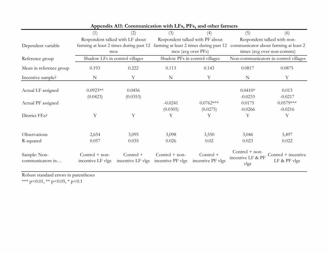
(1) (2) (3) (4) (5) (6)

Dependent variable

Reference group

Mean in reference group 0.193 0.222 0.113 0.143 0.0817 0.0875

Incentive sample? N Y N Y N Y

Actual LF assigned 0.0923** 0.0456 0.0410* 0.013(0.0423) (0.0353) -0.0233 -0.0217

Actual PF assigned -0.0241 0.0762*** 0.0175 0.0579***(0.0305) (0.0275) -0.0266 -0.0216

District FEs? Y Y Y Y Y Y

Observations 2,654 3,095 3,098 3,550 3,046 3,497R-squared 0.057 0.035 0.026 0.02 0.023 0.022

Sample: Non-communicators in…

Control + non-incentive LF vlgs

Control + incentive LF vlgs

Control + non-incentive PF vlgs

Control + incentive PF vlgs

Control + non-incentive LF & PF

vlgs

Control + incentive LF & PF vlgs

Robust standard errors in parentheses*** p<0.01, ** p<0.05, * p<0.1

Appendix A11: Communication with LFs, PFs, and other farmers

Respondent talked with LF about farming at least 2 times during past 12

mos

Respondent talked with PF about farming at least 2 times during past 12

mos (avg over PFs)

Respondent talked with non-communicator about farming at least 2

times (avg over non-comms)

Shadow LFs in control villages Shadow PFs in control villages Non-communicators in control villages

(1) (2) (3)

PFs held demo plot or group training (mean across PFs)

Respondent attended group training led by

PF (mean of PFs)

Respondent attended group training led by

PF (any PF)

0.329** 0.166** 0.195-0.127 -0.0709 -0.1170.023 0.0424 0.0157

-0.0573 -0.0315 -0.0519-0.124 -0.111* -0.0994-0.113 -0.063 -0.0945

District FEs? Y Y YObservations 1,551 1,551 1,551R-squared 0.102 0.075 0.067SampleRobust standard errors in parentheses*** p<0.01, ** p<0.05, * p<0.1

Appendix A12: Communication with LFs, PFs, and other farmers

Incentive village

Respondent farm size smaller or similar than PFs (mean over PFs)Incentive X Farm size smaller or similar to PFs (mean over PFs)

Non-communicators in PF villages

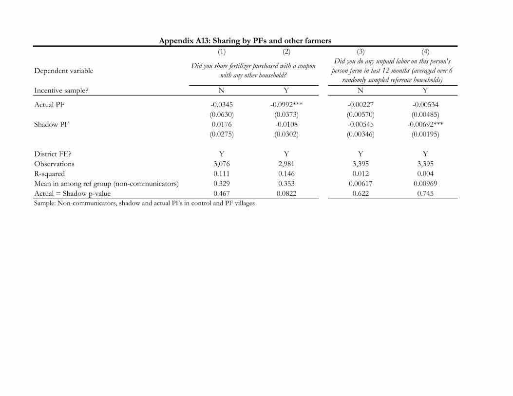
(1) (2) (3) (4)

Dependent variable

Incentive sample? N Y N Y

Actual PF -0.0345 -0.0992*** -0.00227 -0.00534(0.0630) (0.0373) (0.00570) (0.00485)

Shadow PF 0.0176 -0.0108 -0.00545 -0.00692***(0.0275) (0.0302) (0.00346) (0.00195)

District FE? Y Y Y YObservations 3,076 2,981 3,395 3,395R-squared 0.111 0.146 0.012 0.004Mean in among ref group (non-communicators) 0.329 0.353 0.00617 0.00969Actual = Shadow p-value 0.467 0.0822 0.622 0.745Sample: Non-communicators, shadow and actual PFs in control and PF villages

Appendix A13: Sharing by PFs and other farmers

Did you share fertilizer purchased with a coupon with any other household?

Did you do any unpaid labor on this person's person farm in last 12 months (averaged over 6

randomly sampled reference households)

(1) (2) (3) (4)

Respondents

Sample Non-incentive Incentive Non-incentive Incentive

Dependent variable

Actual LF 0.228** 0.382*** 109.5 192.1***(0.106) (0.0975) (66.00) (63.95)

Shadow LF 0.0691 0.0908 59.43** 25.50(0.0707) (0.0860) (26.34) (29.90)

Actual PF 0.0519 0.256*** 28.18 43.94*(0.0699) (0.0619) (21.09) (24.25)

AEDO village

LF village

PF village

Observations 379 372 379 372R-squared 0.071 0.180 0.104 0.141Robust standard errors clus*** p<0.01, ** p<0.05, * p<

Table A14: Continuous Outcome Measures

Communicators

Household produced at least compost heap

Kg of compost produced by HH

Respondents

Sample

Dependent variable

Actual LF

Shadow LF

Actual PF

AEDO village

LF village

PF village

ObservationsR-squaredRobust standard errors clus*** p<0.01, ** p<0.05, * p<

(5) (6) (7) (8) (9) (10) (11) (12) (13) (14) (15) (16)

Non-incentive

IncentiveNon-

incentiveIncentive

Non-incentive

IncentiveNon-

incentiveIncentive

Non-incentive

IncentiveNon-

incentiveIncentive

-0.0834* 0.182* -5.309 12.51-0.0475 -0.0941 -5.14 -8.384-0.0175 0.159** -0.965 7.26 0.207*** 0.281*** 0.257*** 0.315***-0.0686 -0.0751 -6.952 -5.988 (0.0565) (0.0530) (0.0922) (0.0827)-0.0926* 0.280*** -6.982 10.44* 0.125** 0.345*** 0.132 1.355***-0.0531 -0.072 -5.648 -5.762 (0.0496) (0.0620) (0.214) (0.347)

1,600 1,676 1,600 1,676 4,836 4,863 4,836 4,863 4,811 4,845 4,836 4,8630.028 0.071 0.026 0.027 0.148 0.097 0.089 0.122 0.095 0.048 0.041 0.064

Number of activities led by LF respondent

attended

Number of activities led by a PF respondent

attended

Table A14 (continued): Continuous Outcome Measures

Non-communicators

Household produced at least compost heap

Kg of compost produced by HH

LF conducted at least one activity

PF conducted at least one activity

Dependent variable: Household adopted target technology in 2010/11 season

PF has smaller farm than

respondent

PF uses same or fewer

inputs than respondent

PF in immediate

family

PF in extended

family

PF in group with

respondent

Respondent talks daily with PF

(1) (2) (3) (4) (5) (6)

0.0759 0.0707 0.0785 0.0872 0.0727 0.0741(0.0538) (0.0529) (0.0514) (0.0526) (0.0531) (0.0525)0.0808** 0.0792** 0.0724** 0.0872*** 0.0741** 0.0847**(0.0325) (0.0330) (0.0341) (0.0305) (0.0312) (0.0342)0.0738 0.145 0.161*** 0.182*** 0.0854* 0.191***

(0.0962) (0.0884) (0.0395) (0.0575) (0.0502) (0.0431)0.120

(0.200)0.120

(0.180)-0.0116(0.185)

0.110

(0.124)0.225

(0.202)-0.0137(0.116)

Observations 2,193 2,193 2,193 2,193 2,193 2,193R-squared 0.265 0.262 0.262 0.263 0.267 0.263

PF treatment X max(PF uses fewer or similar inputs as respondent)

Table A15: Heterogeneity in PF-Incentive Effects Across Measures of Social Proximity

AEDO treatment

LF treatment

PF treatment

PF treatment X max(PF has smaller or equal farm as respondent)

PF treatment X max(PF in respondent's immediate family)PF treatment X max(PF in respondent's extended family)PF treatment X max(PF in group with respondent)PF treatment X max(PF talks daily with respondent)

Standard errors in parentheses. *** p<0.1, ** p<0.05, * p<0.01. Sample includes all non-communicator households in villages where incentives are provided. Standard errors clustered by village in parentheses. All regressions control for district FE and the same set of control variables as in prior tables. Each regression also controls for the main effect (of "smaller farm", "same or fewer inputs", "education",...etc), but only the interaction terms with the PF treatment are shown for brevity.

[1] [2] [3] [4]Adoption Adoption Adoption Adoption

Benchmark SD Range MADM

0.176*** 0.124 0.162** 0.163**(0.0558) (0.0867) (0.0648) (0.0656)

-0.103***(0.0361)0.0866

(0.0844)-0.0479**(0.0206)0.0249

(0.0459)-0.168**(0.0675)0.0776(0.109)

District FE? Y Y Y YObservations 2,235 2,166 2,166 2,166R-squared 0.184 0.192 0.195 0.196Robust standard errors in parentheses.*** p<0.01, ** p<0.05, * p<0.1Sample includes only villages randomly assigned to the Peer Farmer treatment (with or without incentives)

Mean absolute deviation from mean of baseline area under cultivation across PFs

Incentive village X mean absolute deviation

The dependent variable measures adoption of either Pit Planting or Chinese Composting, as reported in the endline survey by respondents.

Table A16: Heterogeneity in PF-Incentive Effects Across Measures of Social Proximity

Incentive village

SD of baseline area under cultivation across PFs

Incentive village X SD of baseline area under cultivation across PFs

Range of baseline area under cultivation across PFs

Incentive village X Range of baseline area under cultivation across PFs

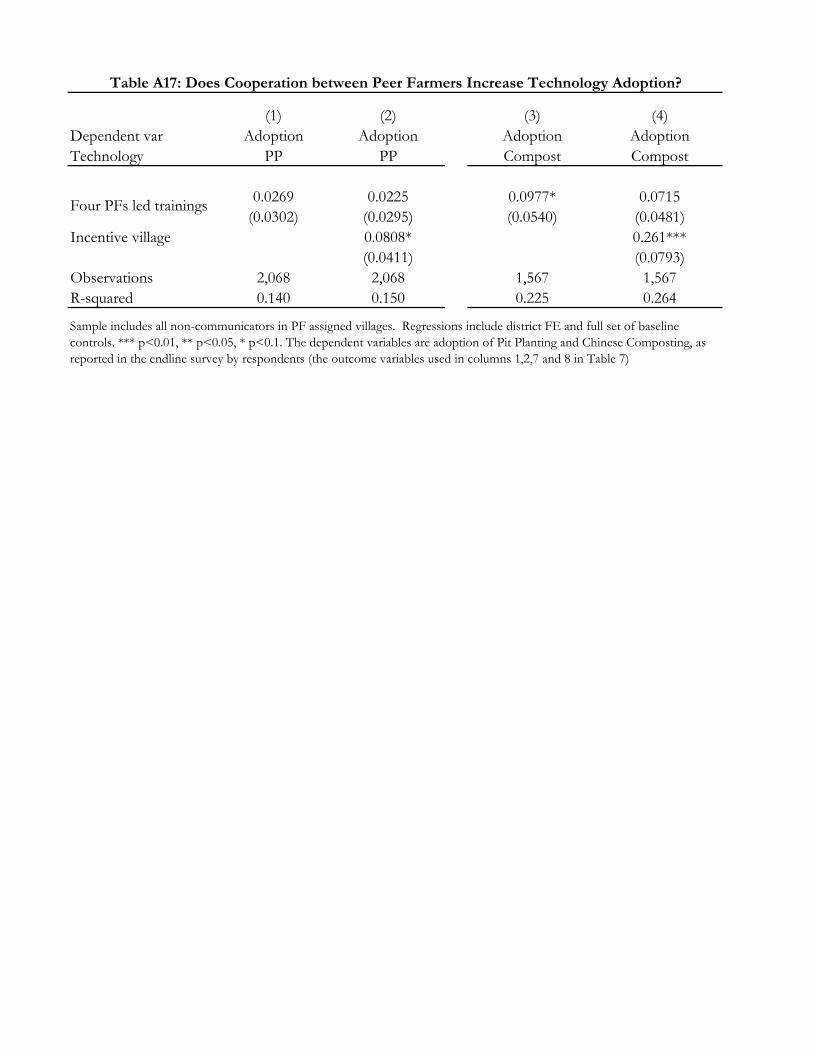
(1) (2) (3) (4)Dependent var Adoption Adoption Adoption AdoptionTechnology PP PP Compost Compost

0.0269 0.0225 0.0977* 0.0715(0.0302) (0.0295) (0.0540) (0.0481)

Incentive village 0.0808* 0.261***(0.0411) (0.0793)

Observations 2,068 2,068 1,567 1,567R-squared 0.140 0.150 0.225 0.264

Table A17: Does Cooperation between Peer Farmers Increase Technology Adoption?

Four PFs led trainings

Sample includes all non-communicators in PF assigned villages. Regressions include district FE and full set of baseline controls. *** p<0.01, ** p<0.05, * p<0.1. The dependent variables are adoption of Pit Planting and Chinese Composting, as reported in the endline survey by respondents (the outcome variables used in columns 1,2,7 and 8 in Table 7)