Embed Size (px)
Citation preview

Social Network Analysis in PythonEnrico Franchi ([email protected])Dipartimento Ingegneria dell’InformazioneUniversità degli Studi di Parma

Outline
Introduction
Data representation
Network Properties
Network Level
Group Level
Node Level
Visualization
PageRank

Social Network Analysis
in Python
Social Network Analysis
in Python
“A social network is a finite set of actors and the relations defined on them”
“A social network is a finite set of actors and the relations defined on them”
NETWORK
“A social network is a finite set of actors and the relations defined on them”
NETWORK
PEOPLE [ACTORS]
“A social network is a finite set of actors and the relations defined on them”
NETWORK
PEOPLE [ACTORS]CONNECTIONS [RELATIONS]
Social Network Analysis
in Python
Social Network Analysis
in Python
Social Network Analysis analyzes the structure of relations among (social, political, organizational) actors
Social Network Analysis
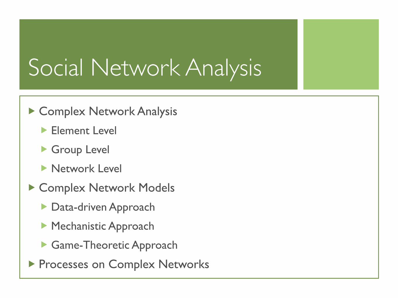
Complex Network Analysis
Element Level
Group Level
Network Level
Complex Network Models
Data-driven Approach
Mechanistic Approach
Game-Theoretic Approach
Processes on Complex Networks
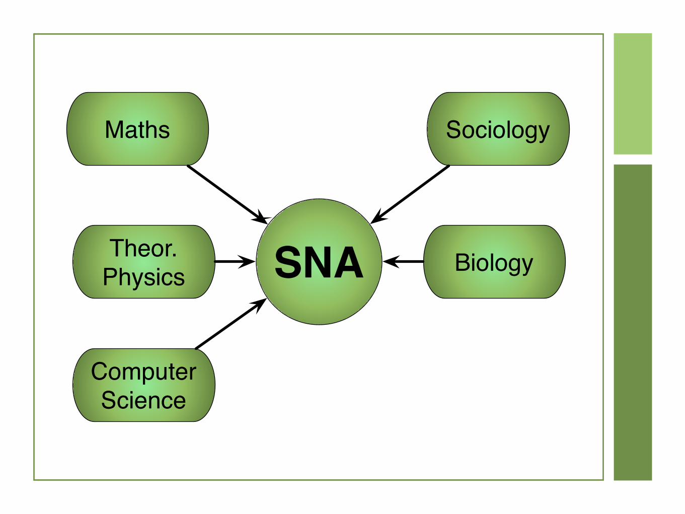
Maths
Theor. Physics
Sociology
Computer Science
BiologySNA

Social Network Analysis
in Python
Social Network Analysis
in Python
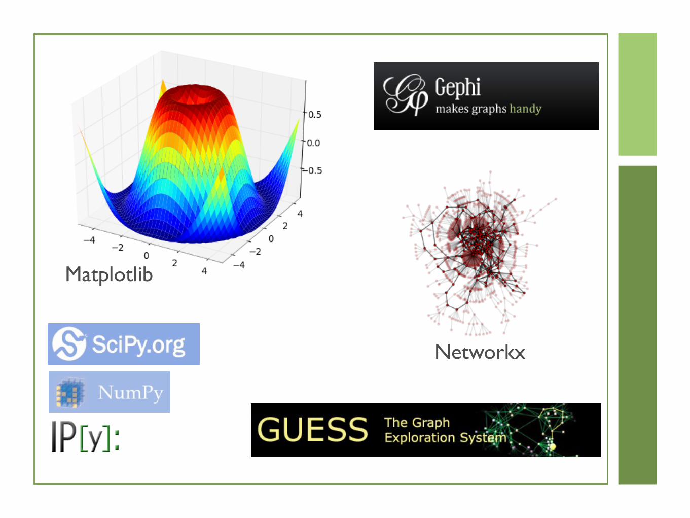
Matplotlib
Networkx
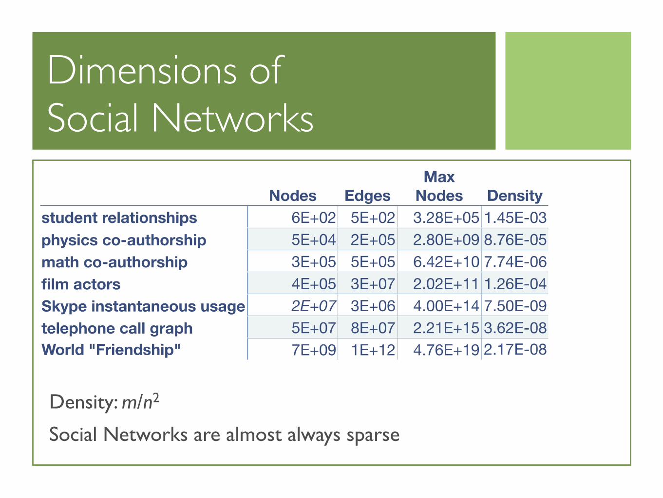
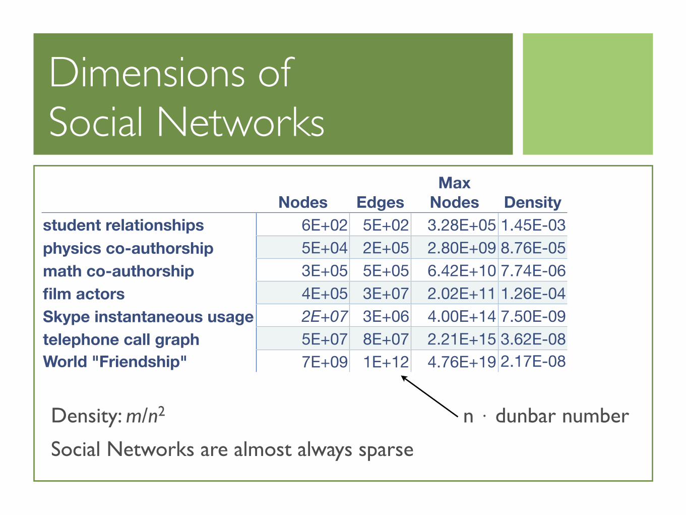
Dimensions ofSocial Networks
Nodes EdgesMax
Nodes Densitystudent relationshipsphysics co-authorshipmath co-authorshipfilm actorsSkype instantaneous usagetelephone call graphWorld "Friendship"
6E+02 5E+02 3.28E+05 1.45E-035E+04 2E+05 2.80E+09 8.76E-053E+05 5E+05 6.42E+10 7.74E-064E+05 3E+07 2.02E+11 1.26E-042E+07 3E+06 4.00E+14 7.50E-095E+07 8E+07 2.21E+15 3.62E-087E+09 1E+12 4.76E+19 2.17E-08
Density: m/n2
Social Networks are almost always sparse
n ⋅ dunbar number
Data Representation
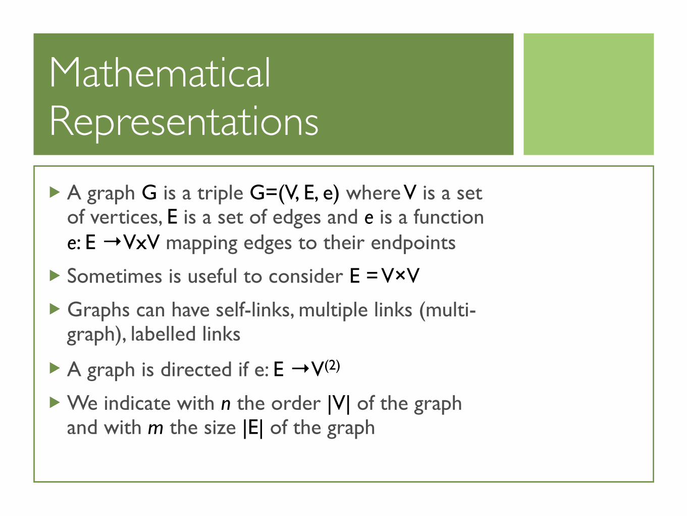
Mathematical Representations
A graph G is a triple G=(V, E, e) where V is a set of vertices, E is a set of edges and e is a function e: E →VxV mapping edges to their endpoints
Sometimes is useful to consider E = V×V
Graphs can have self-links, multiple links (multi-graph), labelled links
A graph is directed if e: E →V(2)
We indicate with n the order |V| of the graph and with m the size |E| of the graph
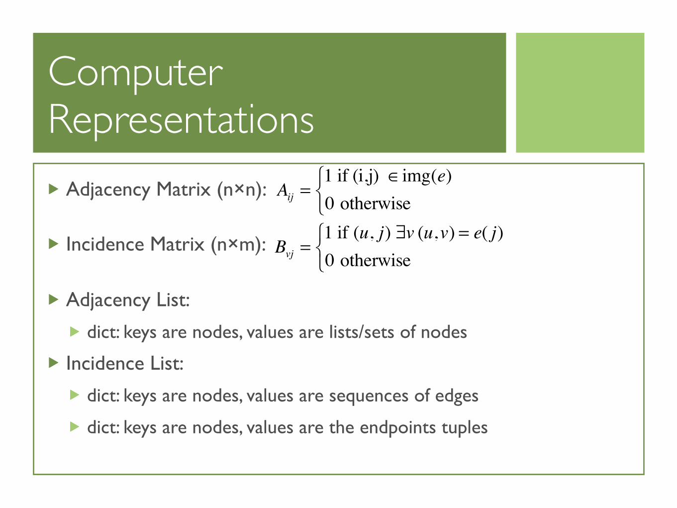
Computer Representations
Adjacency Matrix (n×n):
Incidence Matrix (n×m):
Adjacency List:
dict: keys are nodes, values are lists/sets of nodes
Incidence List:
dict: keys are nodes, values are sequences of edges
dict: keys are nodes, values are the endpoints tuples
Aij =1 if (i,j) ∈img(e)0 otherwise
⎧⎨⎩
Bvj =1 if (u, j) ∃v (u,v) = e( j)0 otherwise
⎧⎨⎩
Sparse Matrices
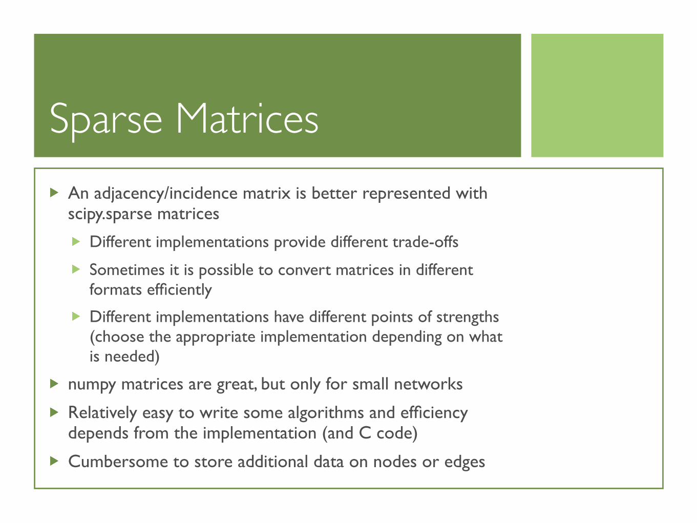
An adjacency/incidence matrix is better represented with scipy.sparse matrices
Different implementations provide different trade-offs
Sometimes it is possible to convert matrices in different formats efficiently
Different implementations have different points of strengths (choose the appropriate implementation depending on what is needed)
numpy matrices are great, but only for small networks
Relatively easy to write some algorithms and efficiency depends from the implementation (and C code)
Cumbersome to store additional data on nodes or edges

Incidence List
This is how graphs are represented in Jung (a widespread Java library which can be used with Jython)
Egde objects are “reified” (contain attributes)
Node objects usually contain attributes as well
“Very OO” [ perhaps an overkill ]
Following the definition leads to inefficiencies
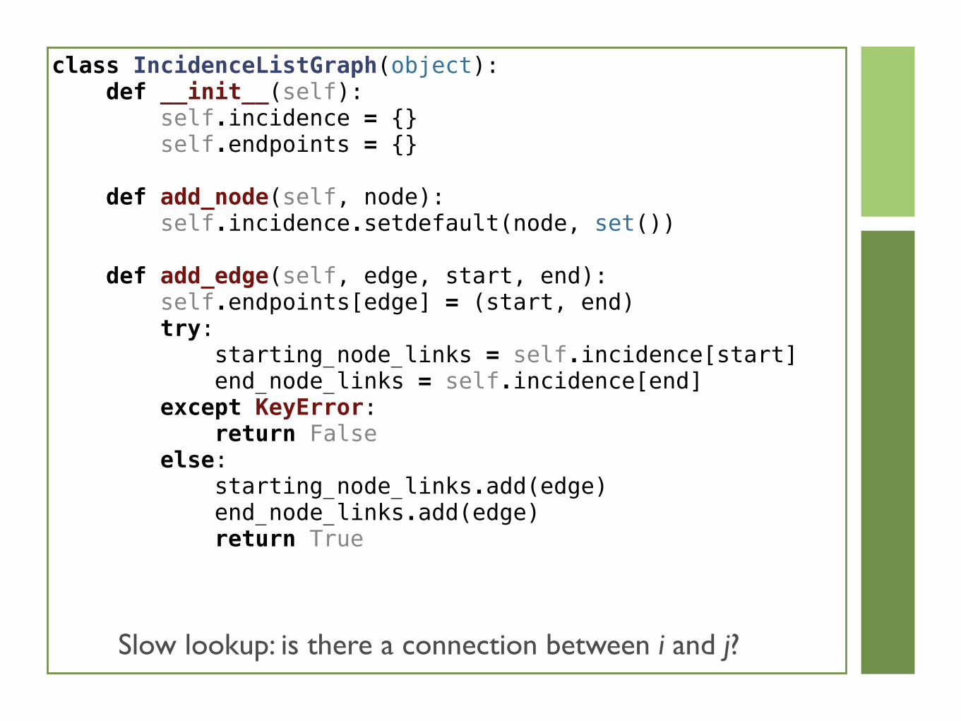
class IncidenceListGraph(object): def __init__(self): self.incidence = {} self.endpoints = {}
def add_node(self, node): self.incidence.setdefault(node, set())
def add_edge(self, edge, start, end): self.endpoints[edge] = (start, end) try: starting_node_links = self.incidence[start] end_node_links = self.incidence[end] except KeyError: return False else: starting_node_links.add(edge) end_node_links.add(edge) return True
Slow lookup: is there a connection between i and j?
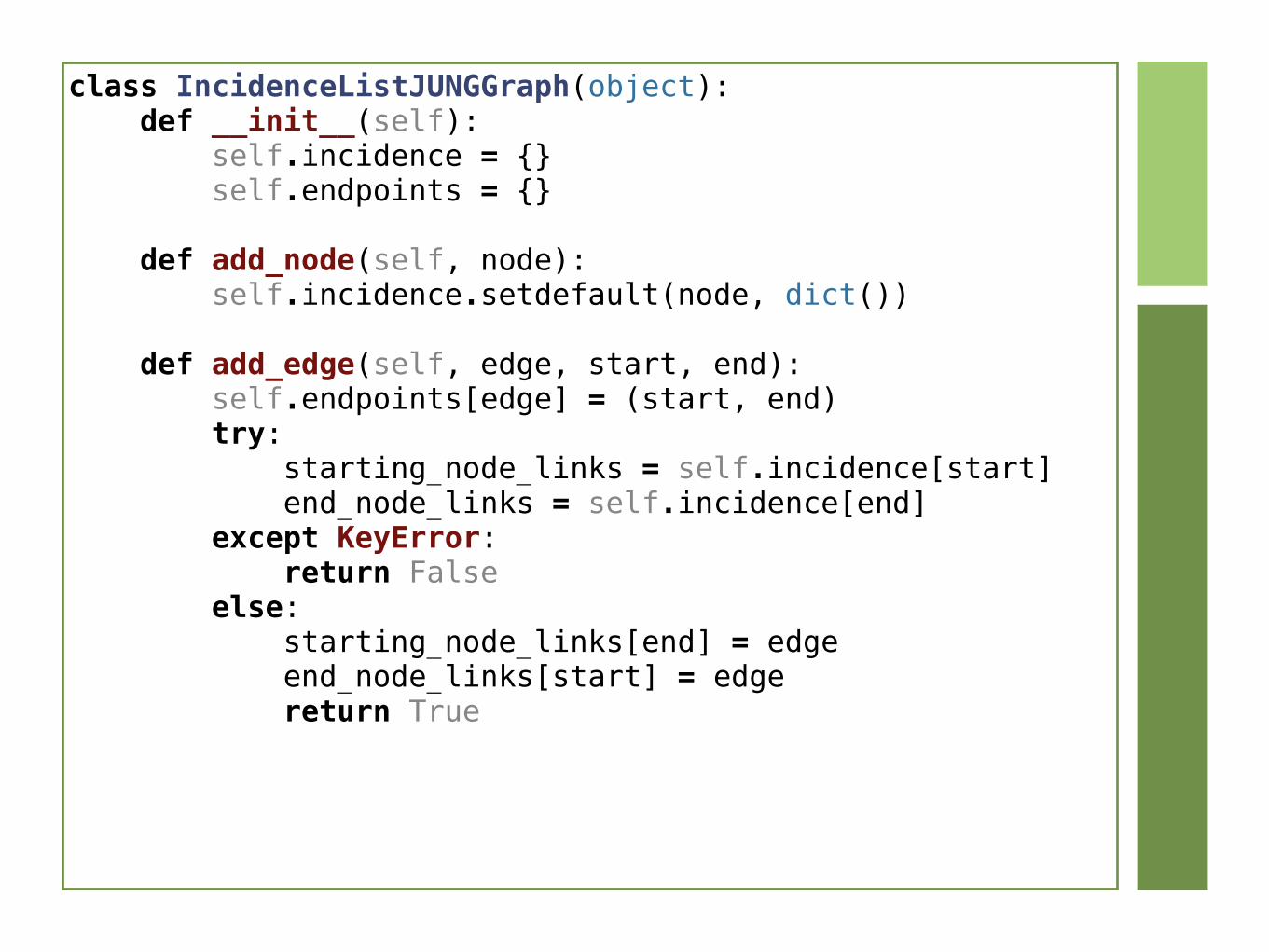
class IncidenceListJUNGGraph(object): def __init__(self): self.incidence = {} self.endpoints = {}
def add_node(self, node): self.incidence.setdefault(node, dict())
def add_edge(self, edge, start, end): self.endpoints[edge] = (start, end) try: starting_node_links = self.incidence[start] end_node_links = self.incidence[end] except KeyError: return False else: starting_node_links[end] = edge end_node_links[start] = edge return True

Adjacency List
Somewhat the “more pythonic way” (http://www.python.org/doc/essays/graphs.html)
Rather efficient in terms of space and costs of elementary operations
Networkx implementation of graphs is based on this idea
graph = {'A': ['B', 'C'], 'B': ['C', 'D'], 'C': ['D'], 'D': ['C'], 'E': ['F'], 'F': ['C']}
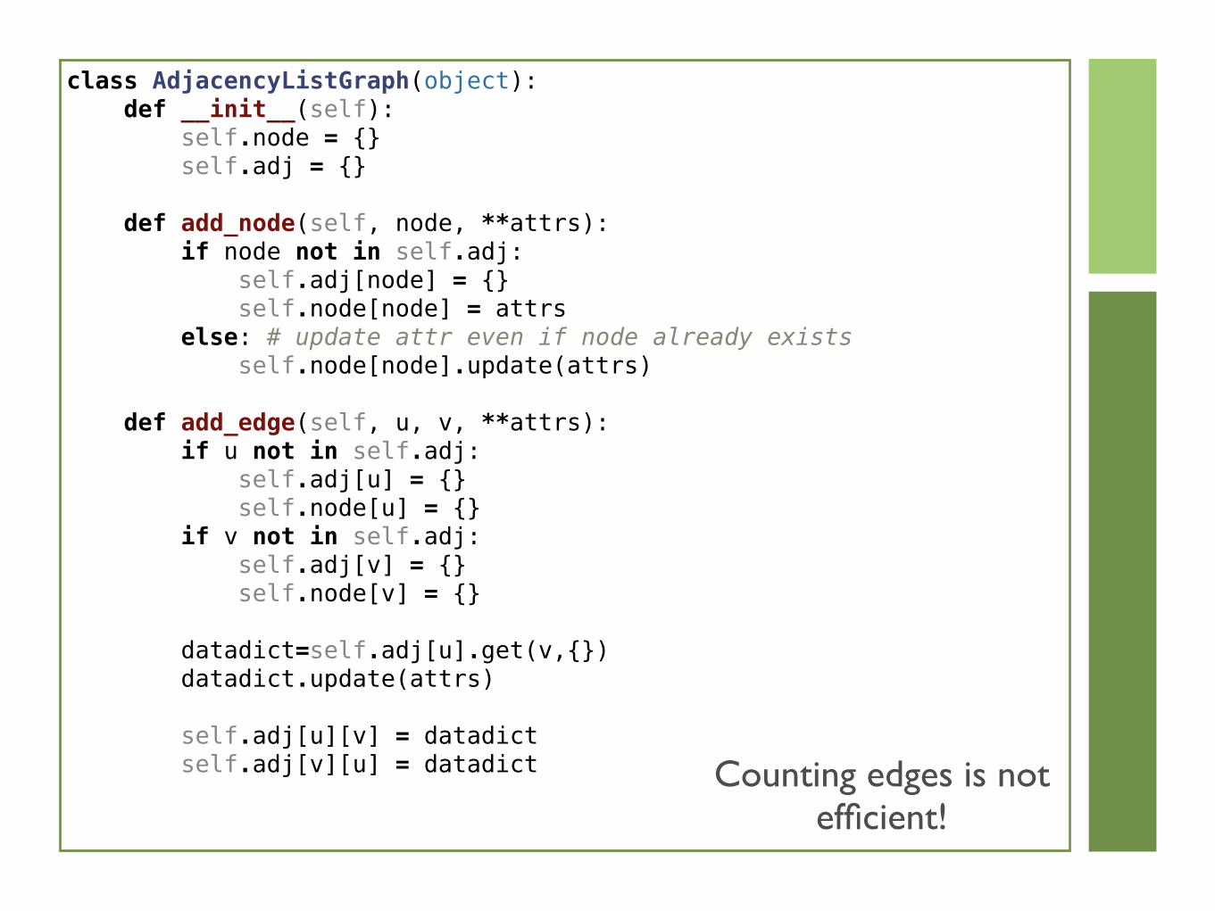
class AdjacencyListGraph(object): def __init__(self): self.node = {} self.adj = {}
def add_node(self, node, **attrs): if node not in self.adj: self.adj[node] = {} self.node[node] = attrs else: # update attr even if node already exists self.node[node].update(attrs)
def add_edge(self, u, v, **attrs): if u not in self.adj: self.adj[u] = {} self.node[u] = {} if v not in self.adj: self.adj[v] = {} self.node[v] = {}
datadict=self.adj[u].get(v,{}) datadict.update(attrs) self.adj[u][v] = datadict self.adj[v][u] = datadict Counting edges is not
efficient!

Graph & File Formats
Networkx graphs can be created from and converted to
numpy matrices
scipy sparse matrices
dicts of lists
dicts of dicts
lists of edges
Networkx graphs can be read from and saved to the following formats
textual formats (adj lists)
GEXF (gephi)
GML
GraphML
Pajek
...

NetworkProperties
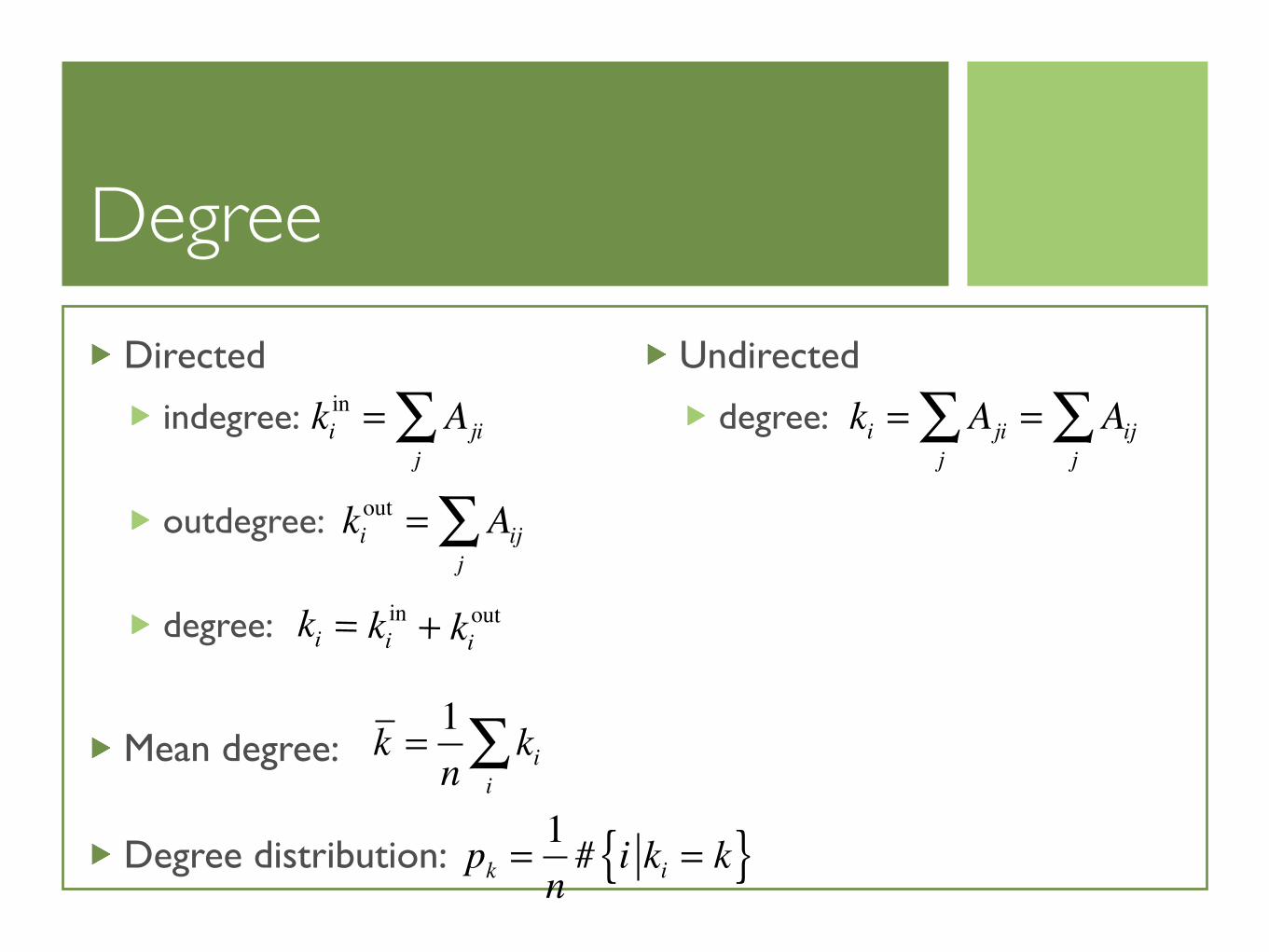
Degree
Directed
indegree:
outdegree:
degree:
Mean degree:
Degree distribution:
Undirected
degree: kiin = Aji
j∑
kiout = Aij
j∑
ki = kiin + ki
out
k = 1n
kii∑
pk =1n# i ki = k{ }
ki = Ajij∑ = Aij
j∑
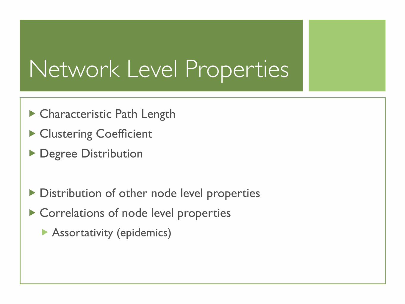
Network Level Properties
Characteristic Path Length
Clustering Coefficient
Degree Distribution
Distribution of other node level properties
Correlations of node level properties
Assortativity (epidemics)
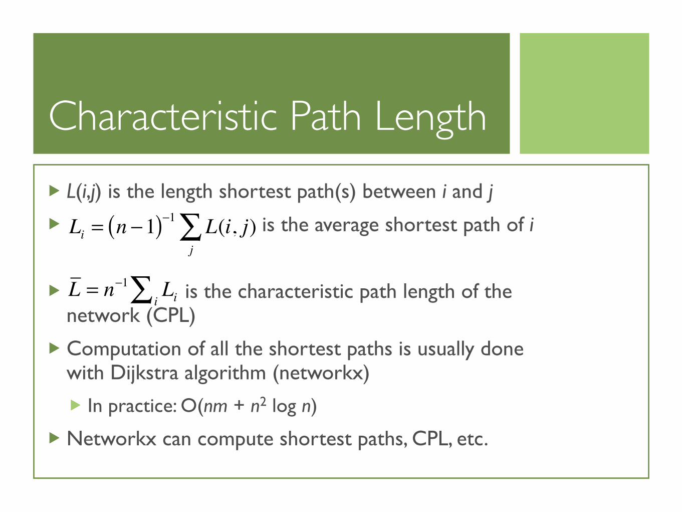
Characteristic Path Length
L(i,j) is the length shortest path(s) between i and j
is the average shortest path of i
is the characteristic path length of the network (CPL)
Computation of all the shortest paths is usually done with Dijkstra algorithm (networkx)
In practice: O(nm + n2 log n)
Networkx can compute shortest paths, CPL, etc.
Li = n −1( )−1 L(i, j)j∑
L = n−1 Lii∑
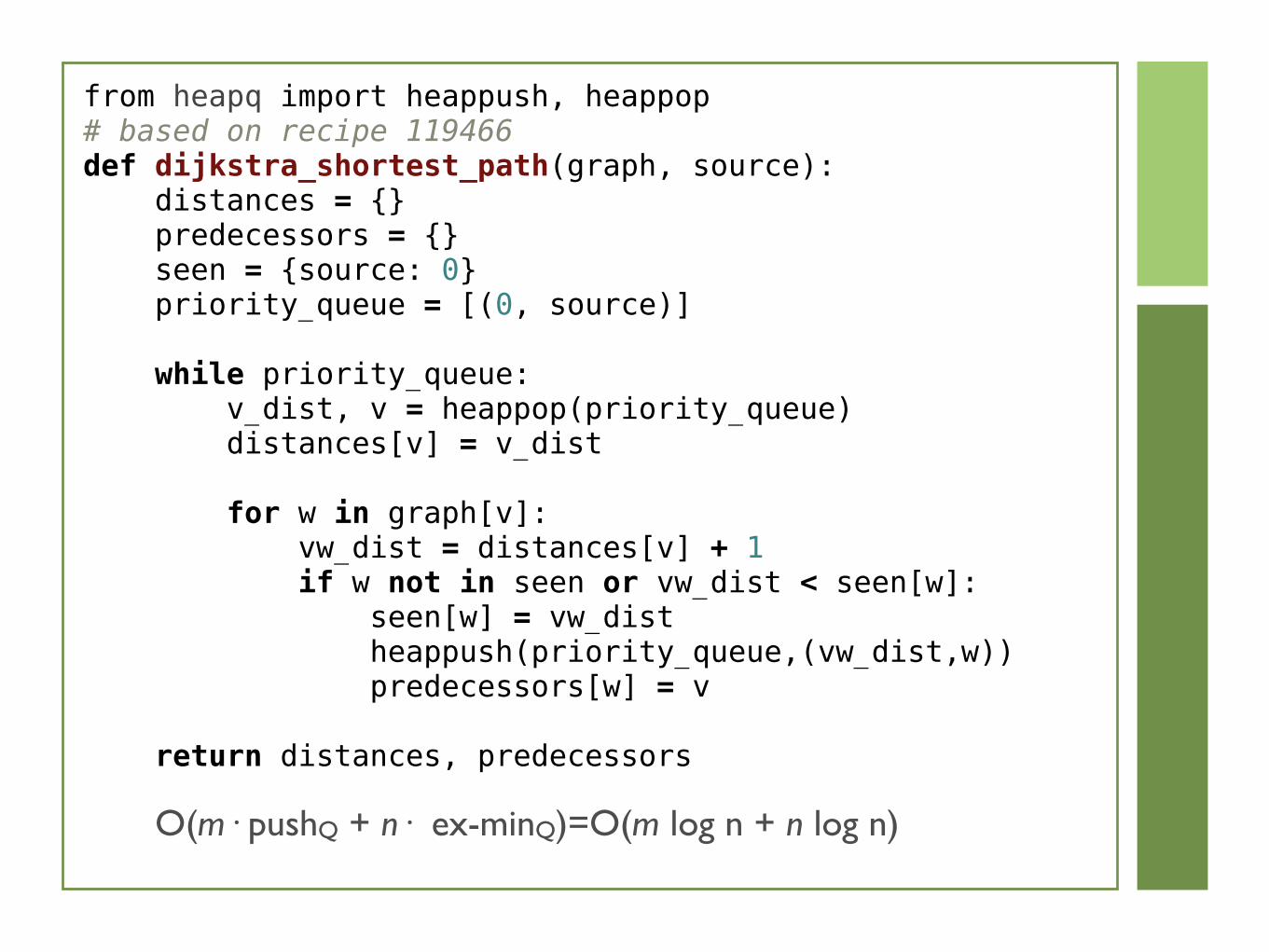
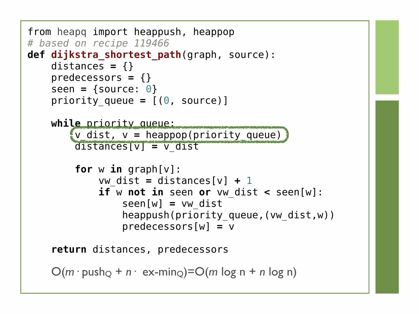
from heapq import heappush, heappop# based on recipe 119466def dijkstra_shortest_path(graph, source): distances = {} predecessors = {} seen = {source: 0} priority_queue = [(0, source)]
while priority_queue: v_dist, v = heappop(priority_queue) distances[v] = v_dist for w in graph[v]: vw_dist = distances[v] + 1 if w not in seen or vw_dist < seen[w]: seen[w] = vw_dist heappush(priority_queue,(vw_dist,w)) predecessors[w] = v
return distances, predecessors
O(m· pushQ + n· ex-minQ)=O(m log n + n log n)
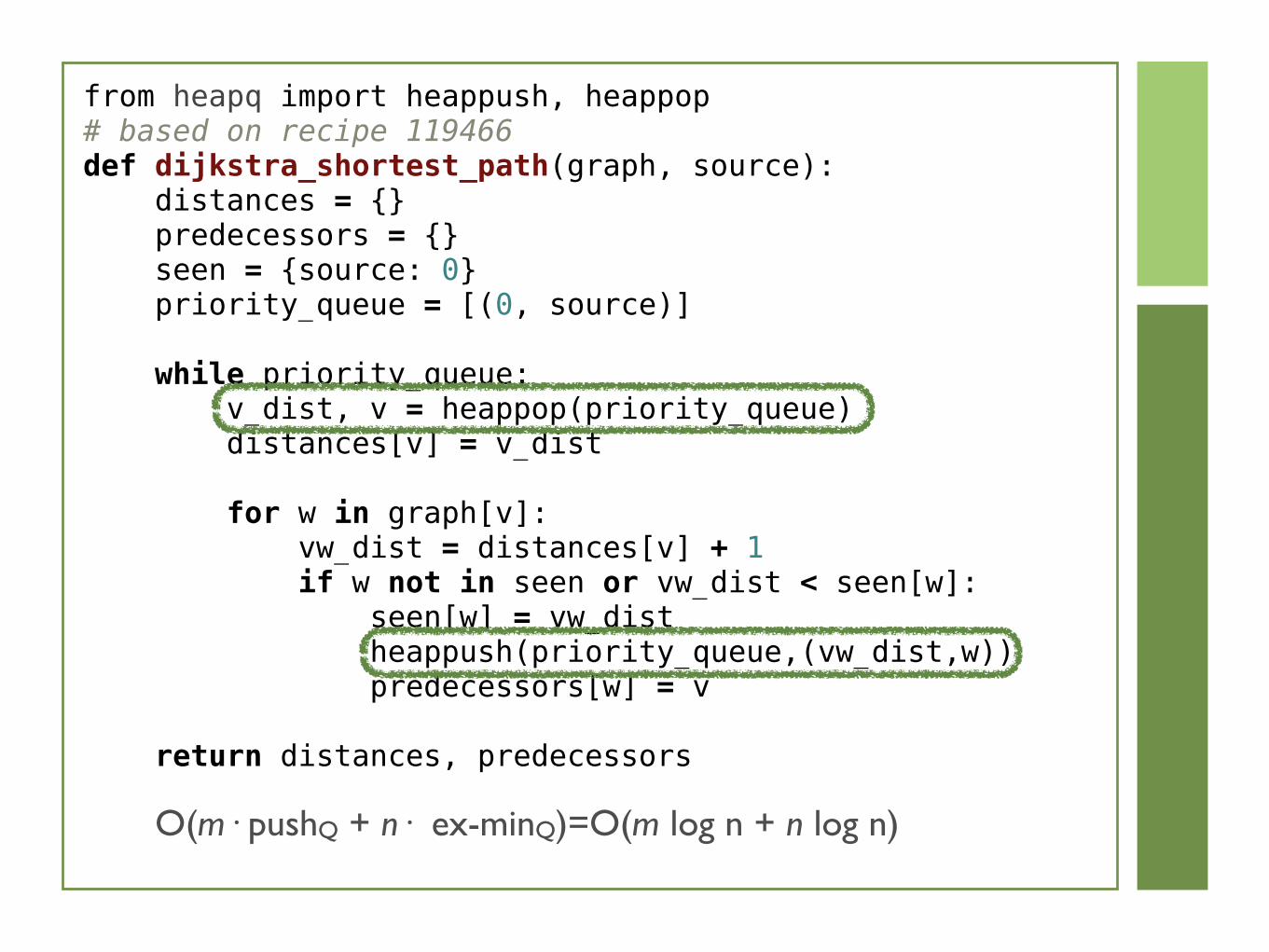
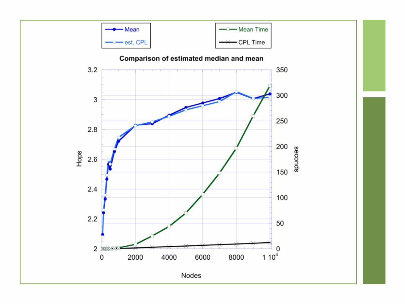
From mean to median
Computing the the shortest paths for all but the smallest networks (< 1000 nodes) is essentially not feasible
However, the median of the average shortest paths is easier to estimate and is a good metric, thus it is common to define the characteristic path length as the median (instead of the mean) of the average shortest path length
Approximate Medians
M(q) is a q-median if at least qn of the numbers in a set are less than or equal to M(q) and at least (1-q)n are greater than M(q)
So a regular median is a 0.5-median
L(q, δ) is a (q, δ)-median if at least qn(1-δ) elements in the set are less than or equal to L(q, δ) and at least (1-q)n(1-δ) are greater than L(q, δ)
Huber Algorithm
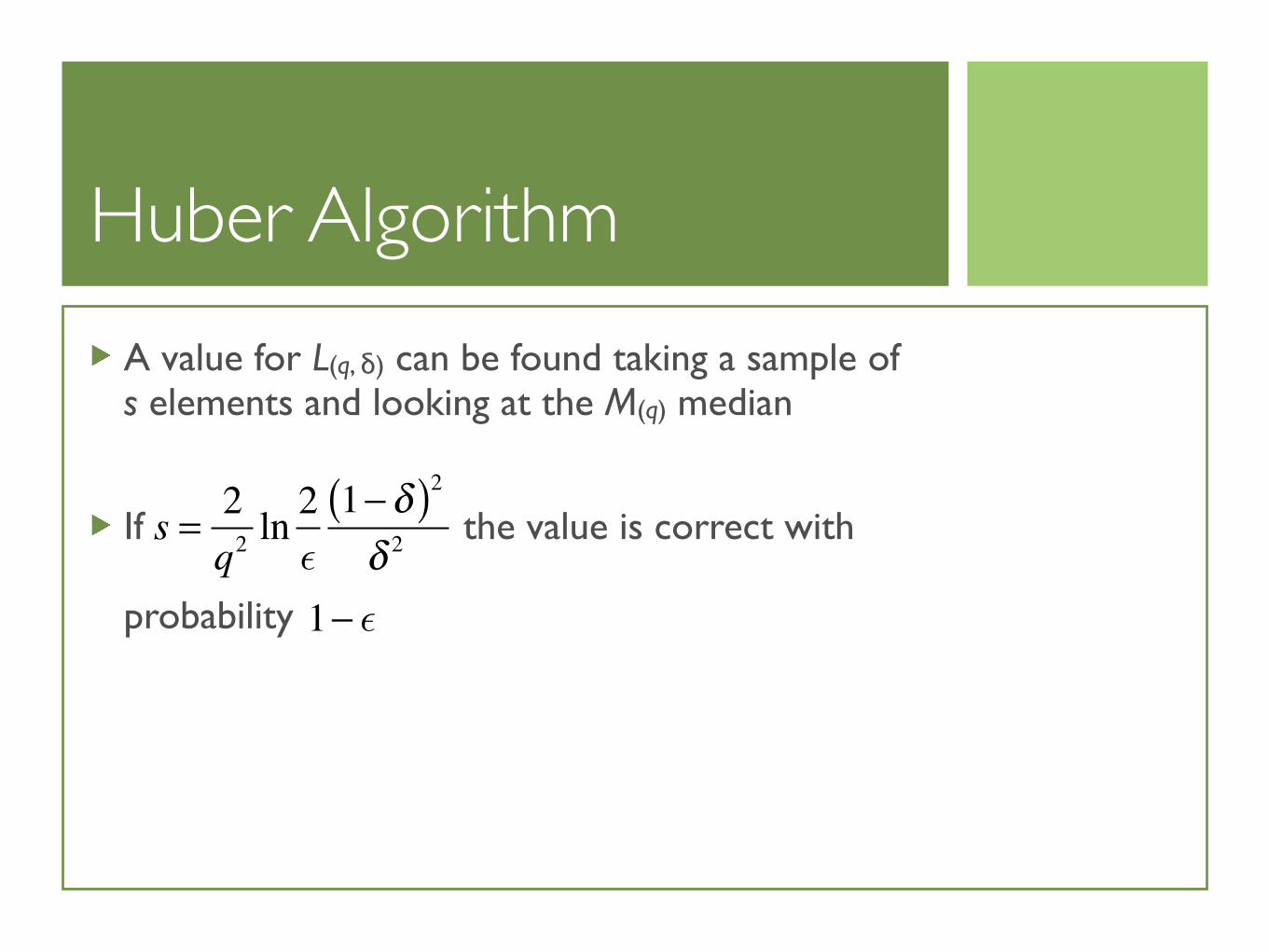
A value for L(q, δ) can be found taking a sample of s elements and looking at the M(q) median
If the value is correct with
probability
s = 2q2ln 2
1−δ( )2δ 2
1−
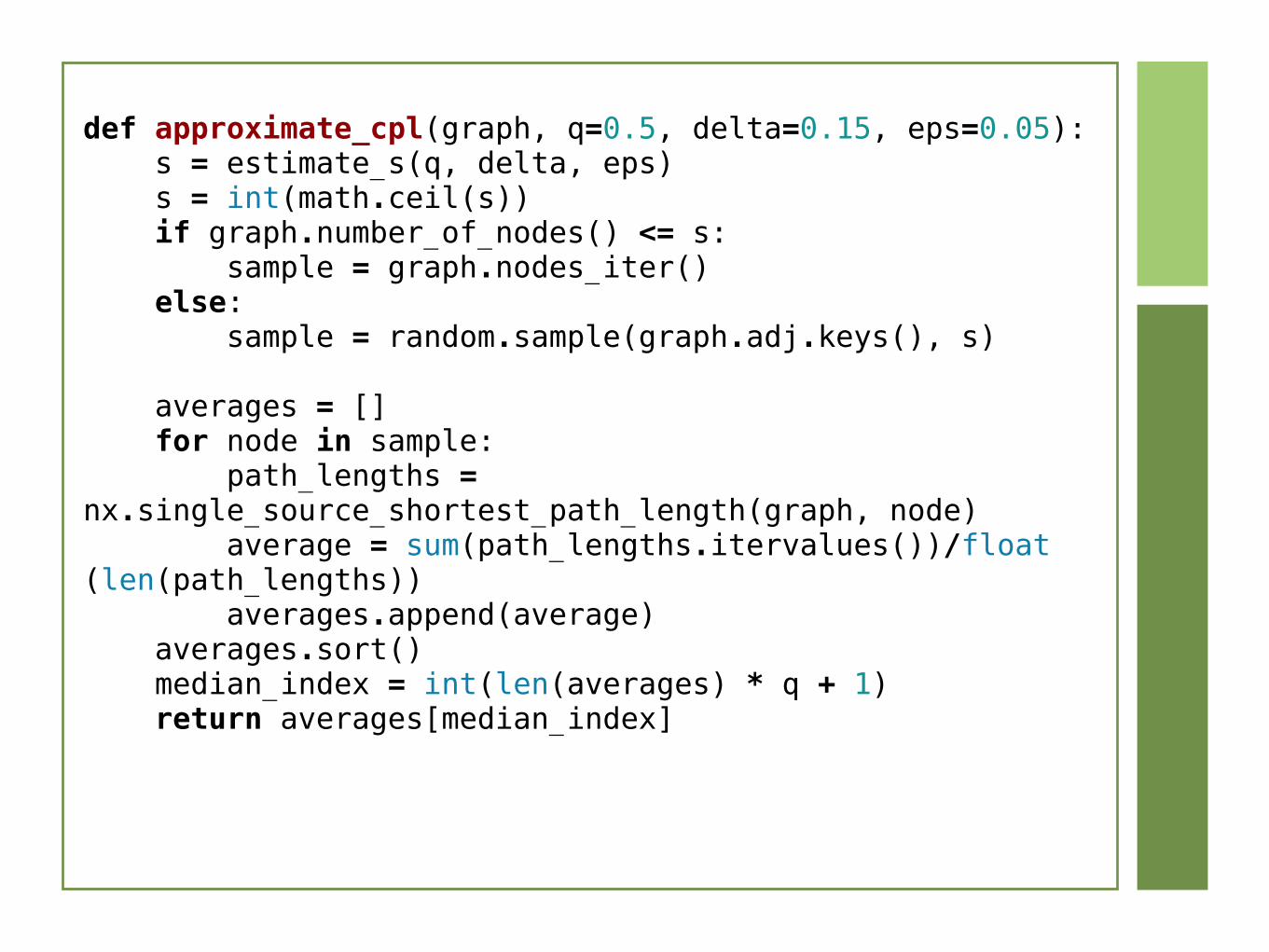
def approximate_cpl(graph, q=0.5, delta=0.15, eps=0.05): s = estimate_s(q, delta, eps) s = int(math.ceil(s)) if graph.number_of_nodes() <= s: sample = graph.nodes_iter() else: sample = random.sample(graph.adj.keys(), s)
averages = [] for node in sample: path_lengths = nx.single_source_shortest_path_length(graph, node) average = sum(path_lengths.itervalues())/float(len(path_lengths)) averages.append(average) averages.sort() median_index = int(len(averages) * q + 1) return averages[median_index]
Local Clustering Coefficient
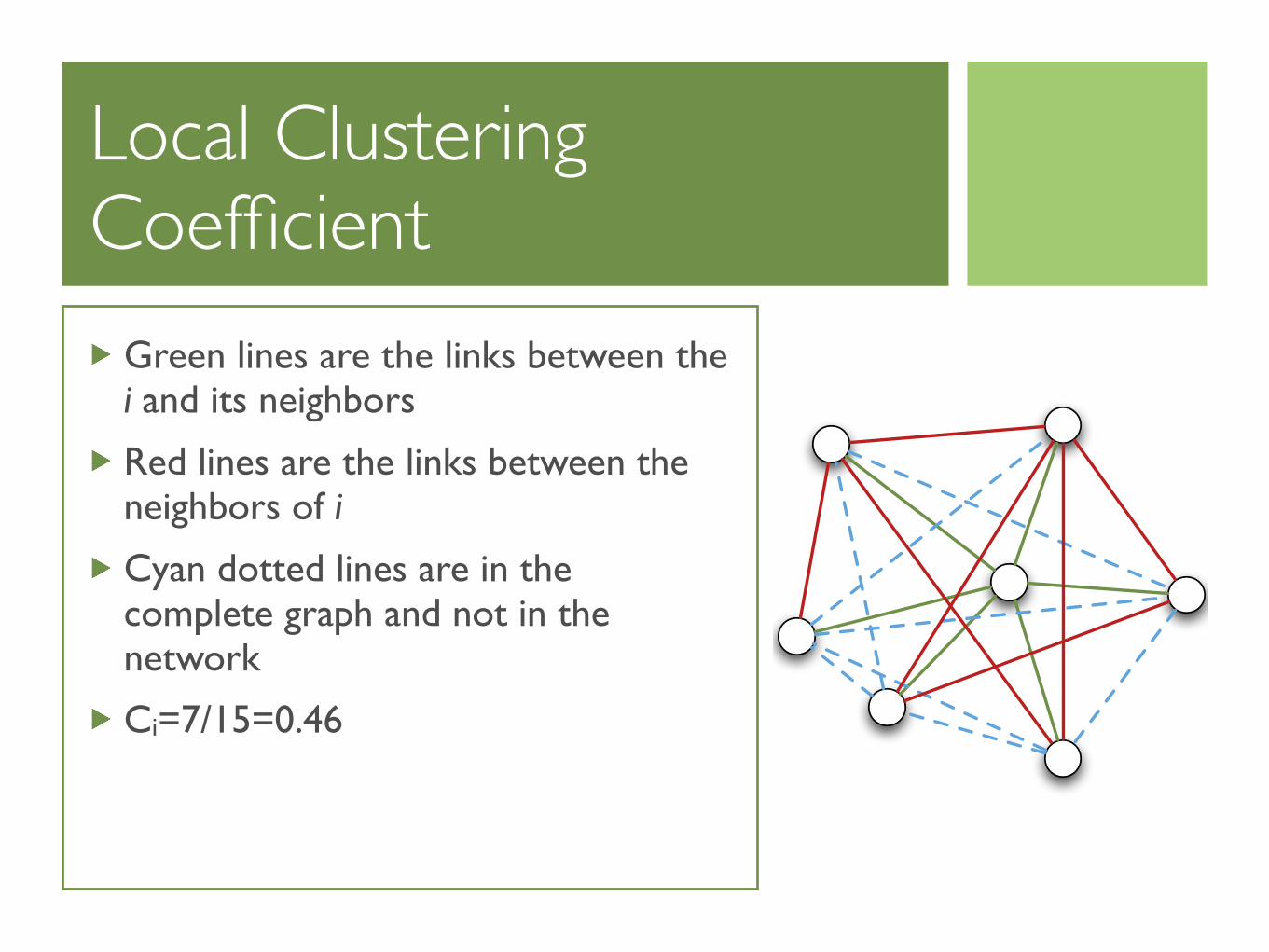
Green lines are the links between the i and its neighbors
Red lines are the links between the neighbors of i
Cyan dotted lines are in the complete graph and not in the network
Ci=7/15=0.46
Local Clustering Coefficient
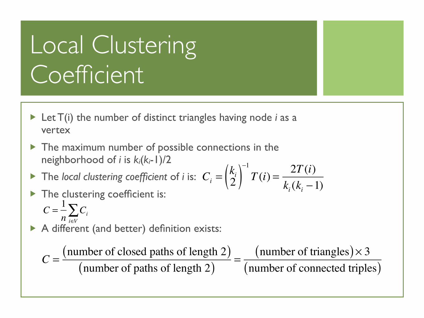
Let T(i) the number of distinct triangles having node i as a vertex
The maximum number of possible connections in the neighborhood of i is ki(ki-1)/2
The local clustering coefficient of i is:
The clustering coefficient is:
A different (and better) definition exists:
Ci =ki2( )−1T (i) = 2T (i)
ki (ki −1)
C = 1n
Cii∈V∑
C =number of closed paths of length 2( )
number of paths of length 2( ) =number of triangles( )× 3
number of connected triples( )
Local Clustering Coefficient
Let T(i) the number of distinct triangles having node i as a vertex
The maximum number of possible connections in the neighborhood of i is ki(ki-1)/2
The local clustering coefficient of i is:
The clustering coefficient is:
A different (and better) definition exists:
Ci =ki2( )−1T (i) = 2T (i)
ki (ki −1)
C = 1n
Cii∈V∑
C =number of closed paths of length 2( )
number of paths of length 2( ) =number of triangles( )× 3
number of connected triples( )
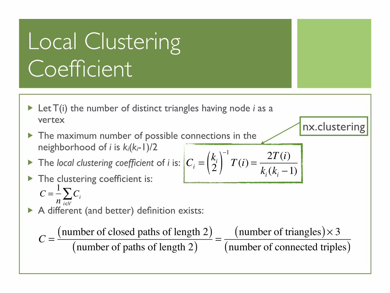
nx.clustering
Local Clustering Coefficient
Let T(i) the number of distinct triangles having node i as a vertex
The maximum number of possible connections in the neighborhood of i is ki(ki-1)/2
The local clustering coefficient of i is:
The clustering coefficient is:
A different (and better) definition exists:
Ci =ki2( )−1T (i) = 2T (i)
ki (ki −1)
C = 1n
Cii∈V∑
C =number of closed paths of length 2( )
number of paths of length 2( ) =number of triangles( )× 3
number of connected triples( )
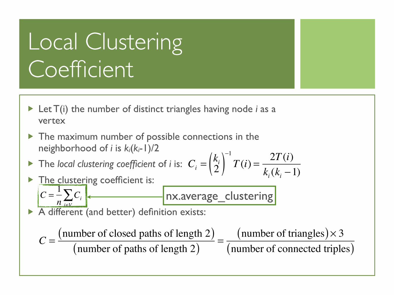
nx.average_clustering
Local Clustering Coefficient
Let T(i) the number of distinct triangles having node i as a vertex
The maximum number of possible connections in the neighborhood of i is ki(ki-1)/2
The local clustering coefficient of i is:
The clustering coefficient is:
A different (and better) definition exists:
Ci =ki2( )−1T (i) = 2T (i)
ki (ki −1)
C = 1n
Cii∈V∑
C =number of closed paths of length 2( )
number of paths of length 2( ) =number of triangles( )× 3
number of connected triples( )
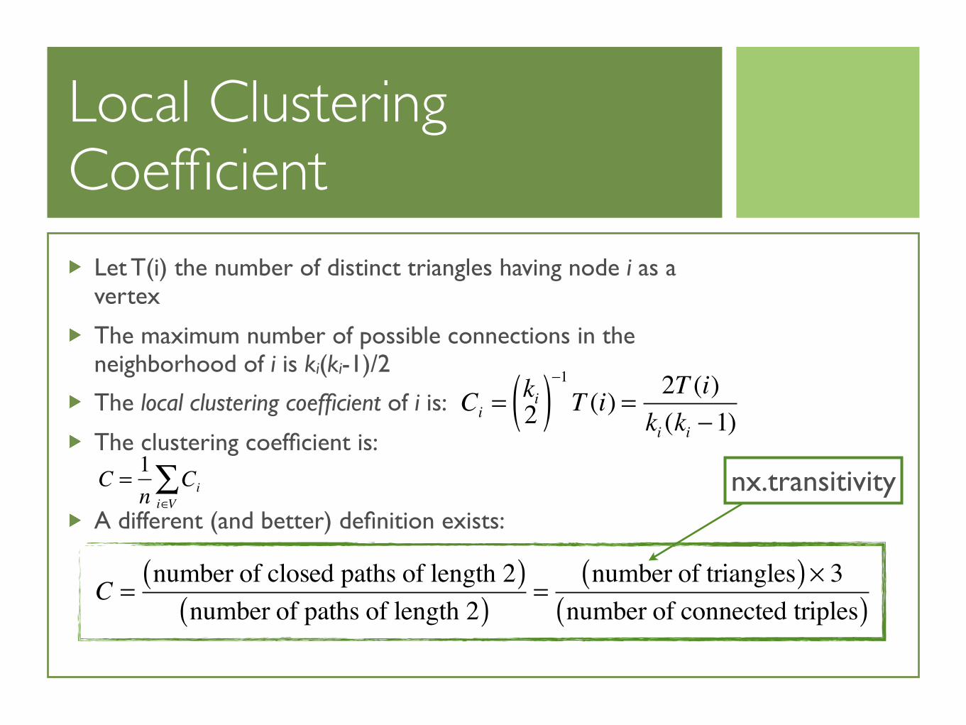
nx.transitivity

Local Clustering Coefficient
Let T(i) the number of distinct triangles having node i as a vertex
The maximum number of possible connections in the neighborhood of i is ki(ki-1)/2
The local clustering coefficient of i is:
The clustering coefficient is:
A different (and better) definition exists:
Ci =ki2( )−1T (i) = 2T (i)
ki (ki −1)
C = 1n
Cii∈V∑
C =number of closed paths of length 2( )
number of paths of length 2( ) =number of triangles( )× 3
number of connected triples( )
Degree Distribution
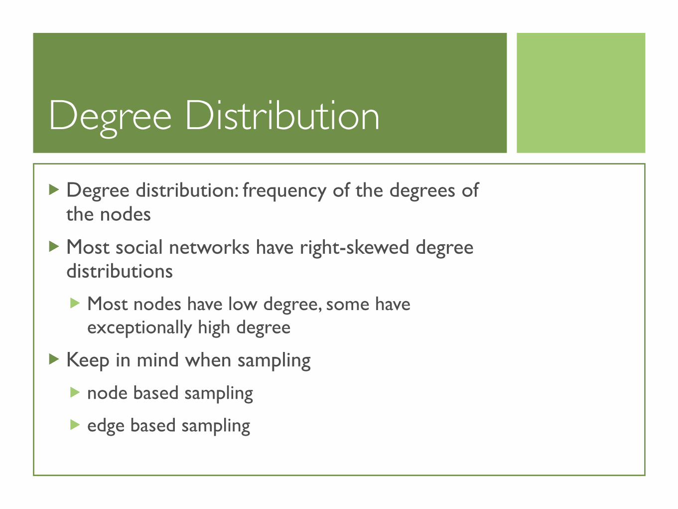
Degree distribution: frequency of the degrees of the nodes
Most social networks have right-skewed degree distributions
Most nodes have low degree, some have exceptionally high degree
Keep in mind when sampling
node based sampling
edge based sampling
Power-Laws
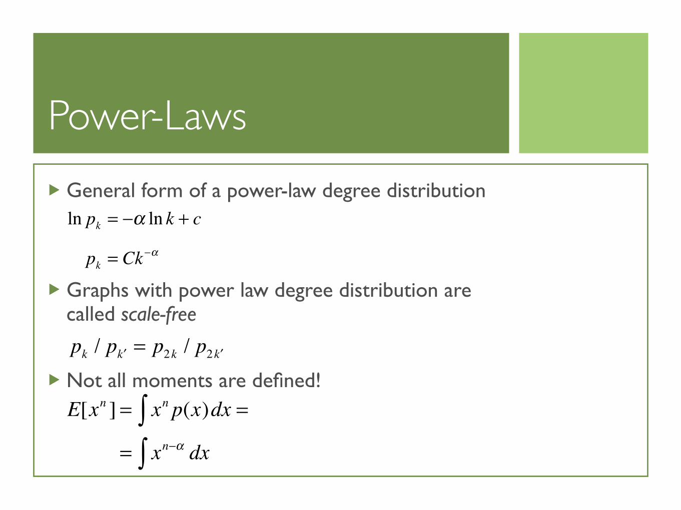
General form of a power-law degree distribution
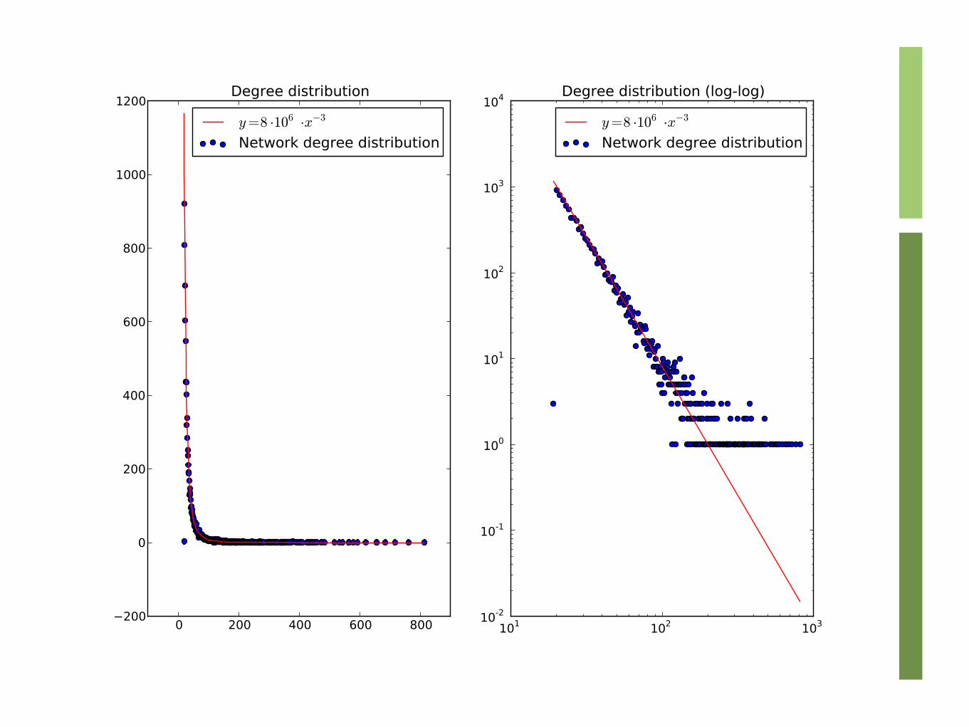
Graphs with power law degree distribution are called scale-free
Not all moments are defined!
ln pk = −α ln k + c
pk = Ck−α
pk / p ′k = p2k / p2 ′k
E[xn ] = xn p(x)dx =∫= xn−α dx∫
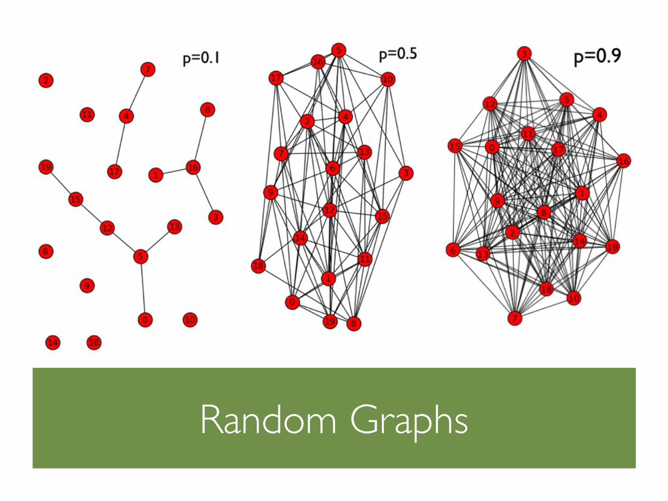
Random Graphs
An Erdös-Rényi random graph model G(n, m) is a probability distribution over the set of simple graphs with n nodes and m edges
A mathematically equivalent model (for large n) is G(n, p). When a graph is drawn from G(n, p) each possible edge is independently placed with probability p
Other than the naive ways to code the process, there are efficient O(n+m) algorithms (implemented in networkx)
Random Graphs
ER-Random Graphs
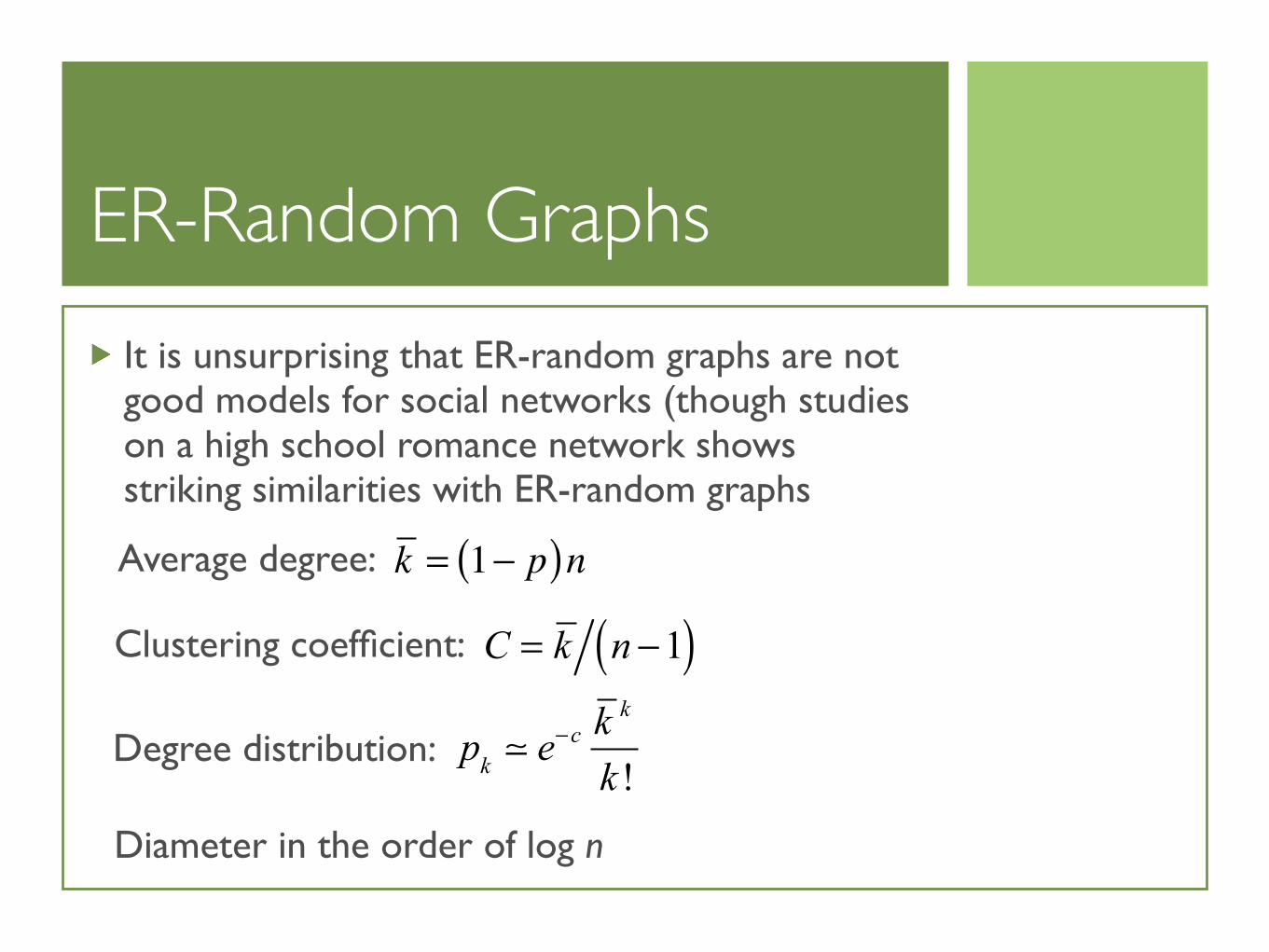
It is unsurprising that ER-random graphs are not good models for social networks (though studies on a high school romance network shows striking similarities with ER-random graphs
C = k n −1( )k = 1− p( )n
pk e−c k k
k !
Average degree:
Clustering coefficient:
Degree distribution:
Diameter in the order of log n
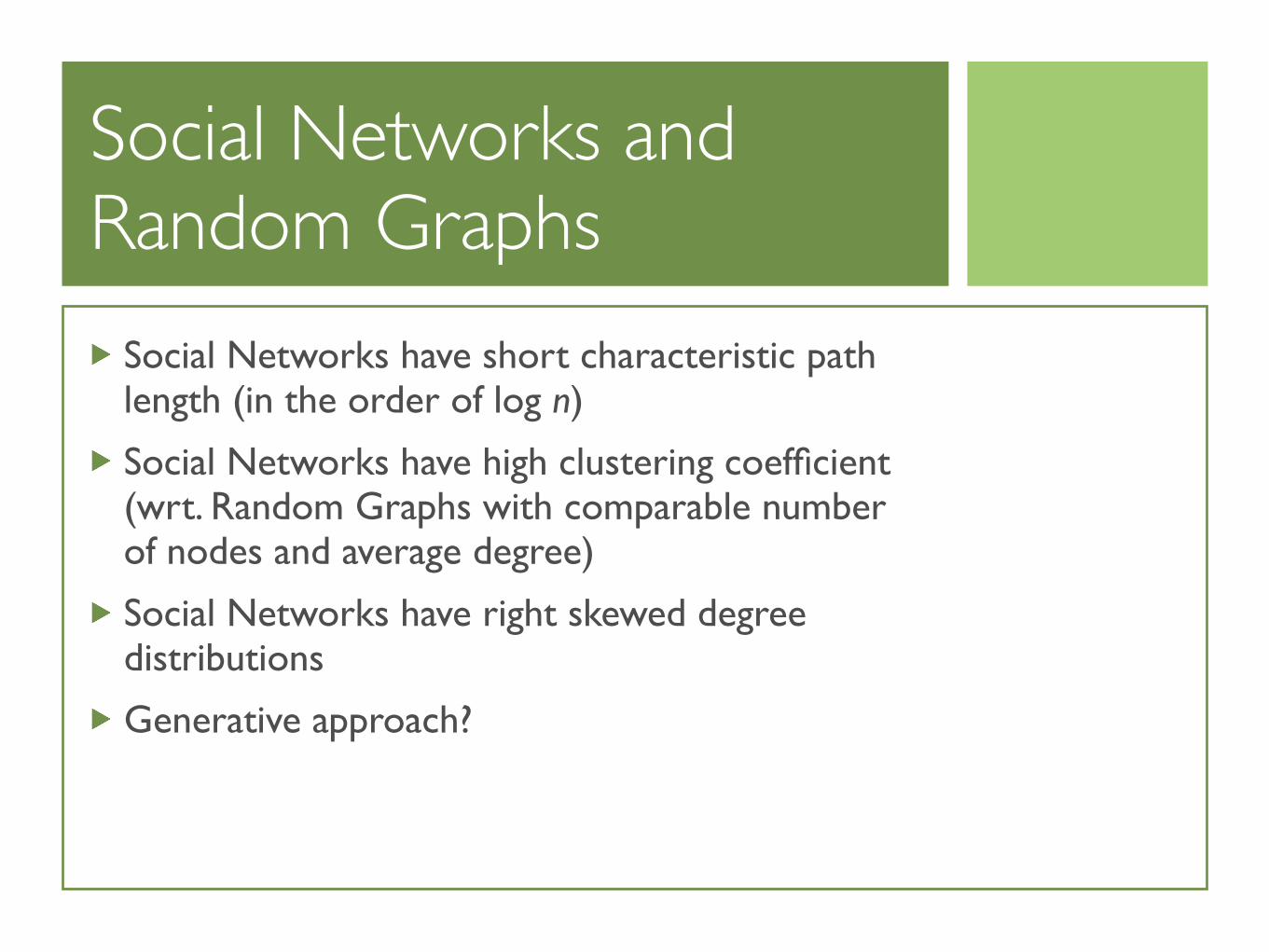
Social Networks and Random Graphs
Social Networks have short characteristic path length (in the order of log n)
Social Networks have high clustering coefficient (wrt. Random Graphs with comparable number of nodes and average degree)
Social Networks have right skewed degree distributions
Generative approach?
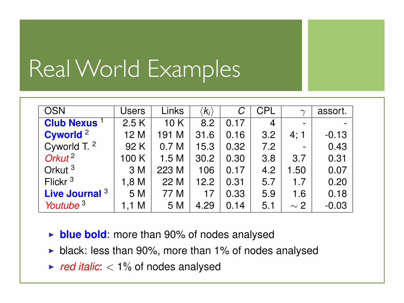
Real World ExamplesReal Online Social Networks
OSN Users Links �ki� C CPL γ assort.
Club Nexus 1 2.5 K 10 K 8.2 0.17 4 - -
Cyworld 2 12 M 191 M 31.6 0.16 3.2 4; 1 -0.13
Cyworld T. 2 92 K 0.7 M 15.3 0.32 7.2 - 0.43
Orkut 2 100 K 1.5 M 30.2 0.30 3.8 3.7 0.31
Orkut 3 3 M 223 M 106 0.17 4.2 1.50 0.07
Flickr 3 1,8 M 22 M 12.2 0.31 5.7 1.7 0.20
Live Journal 3 5 M 77 M 17 0.33 5.9 1.6 0.18
Youtube 3 1,1 M 5 M 4.29 0.14 5.1 ∼ 2 -0.03
� blue bold: more than 90% of nodes analysed
� black: less than 90%, more than 1% of nodes analysed
� red italic: < 1% of nodes analysed
1[Adamic 05]
2[Ahn 07]
3[Mislove 07]
Bergenti, Franchi, Poggi (Univ. Parma) Models for Agent-based Simulation of SN SNAMAS ’11 8 / 19

Group Level Properties
Identification of cohesive sub-groups
one-mode networks (n-clique, n-clan, n-club, k-plex, k-core, LS set)
two-mode networks
Network Positions
Blockmodels
Networkx gives them all!
Efficiency, interpretation

Group Level Properties
Identification of cohesive sub-groups
one-mode networks (n-clique, n-clan, n-club, k-plex, k-core, LS set)
two-mode networks
Network Positions
Blockmodels
Networkx gives them all!
Efficiency, interpretation
Highly connected core
Fringe
Stars & Isolated Nodes

Node level properties
“Centrality” metrics
Ranking
Study distribution & correlation
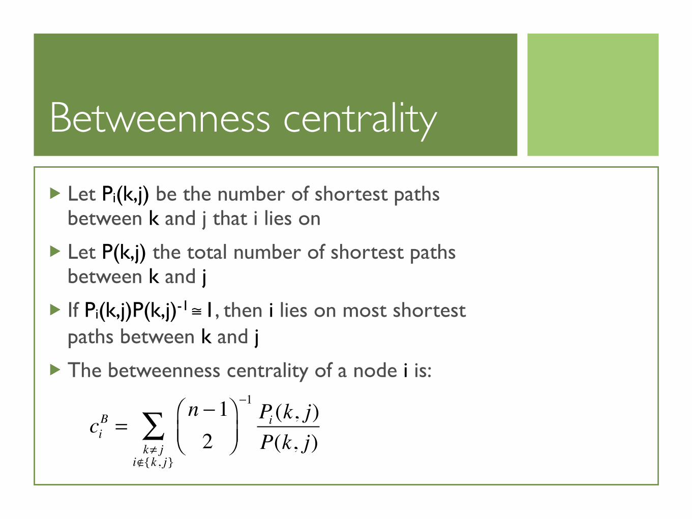
Betweenness centrality
Let Pi(k,j) be the number of shortest paths between k and j that i lies on
Let P(k,j) the total number of shortest paths between k and j
If Pi(k,j)P(k,j)-1≅1, then i lies on most shortest paths between k and j
The betweenness centrality of a node i is:
ciB =
n −12
⎛⎝⎜
⎞⎠⎟
−1Pi (k, j)P(k, j)k≠ j
i /∈{k , j}
∑
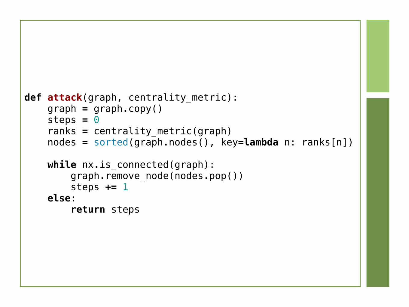
def attack(graph, centrality_metric): graph = graph.copy() steps = 0 ranks = centrality_metric(graph) nodes = sorted(graph.nodes(), key=lambda n: ranks[n])
while nx.is_connected(graph): graph.remove_node(nodes.pop()) steps += 1 else: return steps
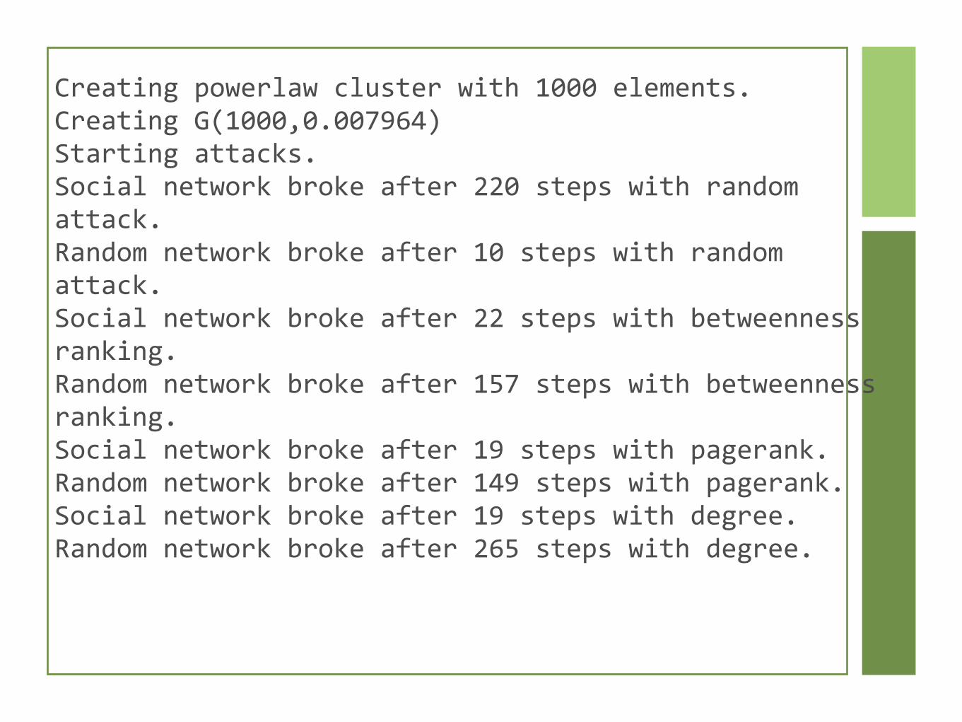
Creating powerlaw cluster with 1000 elements.Creating G(1000,0.007964)Starting attacks.Social network broke after 220 steps with random attack.Random network broke after 10 steps with random attack.Social network broke after 22 steps with betweenness ranking.Random network broke after 157 steps with betweenness ranking.Social network broke after 19 steps with pagerank.Random network broke after 149 steps with pagerank.Social network broke after 19 steps with degree.Random network broke after 265 steps with degree.

Visualization
Visualization
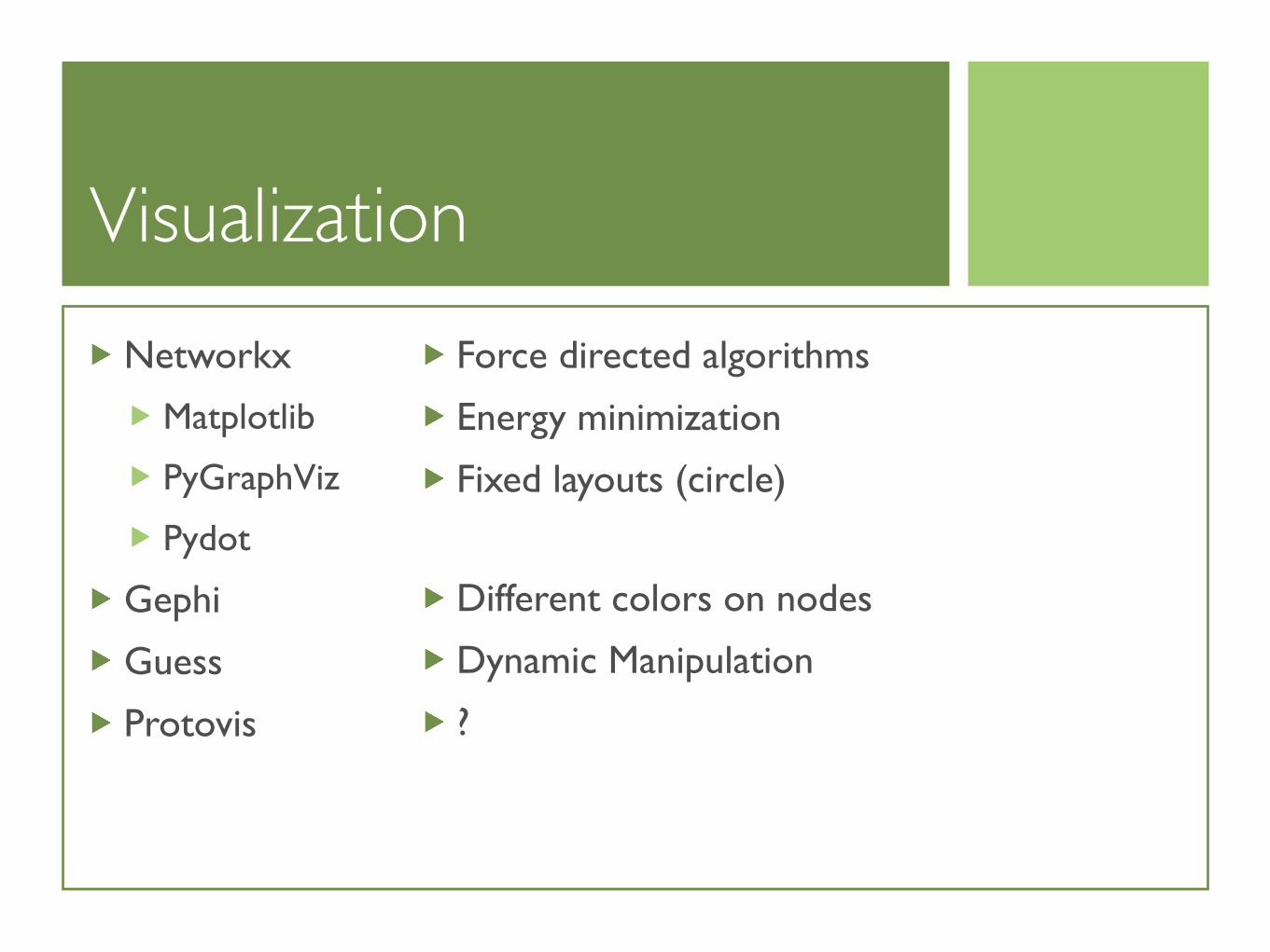
Networkx
Matplotlib
PyGraphViz
Pydot
Gephi
Guess
Protovis
Force directed algorithms
Energy minimization
Fixed layouts (circle)
Different colors on nodes
Dynamic Manipulation
?
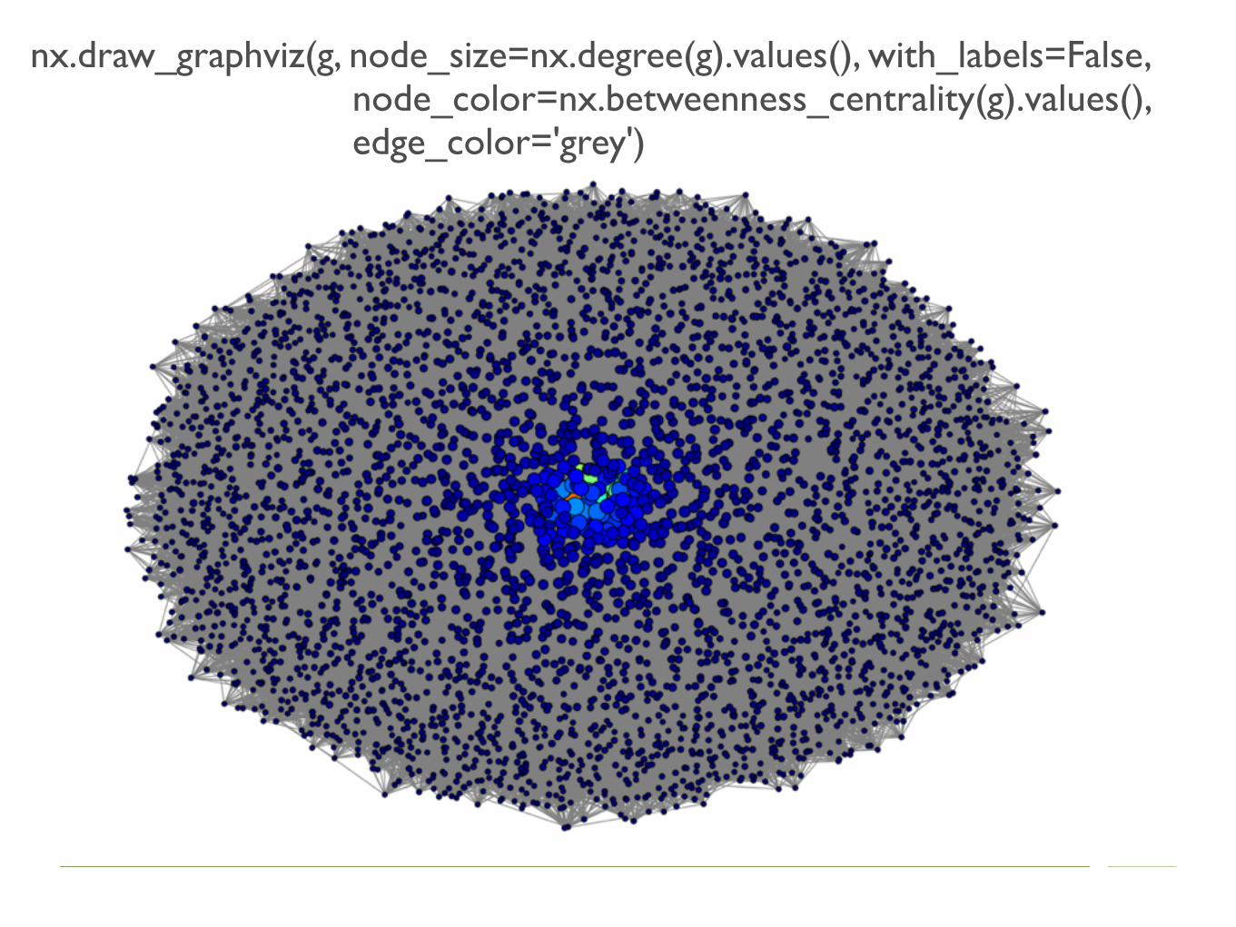
nx.draw_graphviz(g, node_size=nx.degree(g).values(), with_labels=False, node_color=nx.betweenness_centrality(g).values(), edge_color='grey')
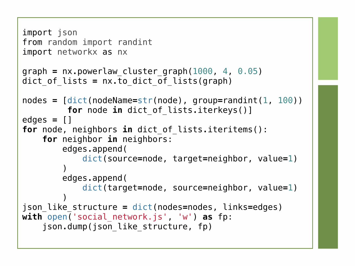
import jsonfrom random import randintimport networkx as nx
graph = nx.powerlaw_cluster_graph(1000, 4, 0.05)dict_of_lists = nx.to_dict_of_lists(graph)
nodes = [dict(nodeName=str(node), group=randint(1, 100)) for node in dict_of_lists.iterkeys()]edges = []for node, neighbors in dict_of_lists.iteritems(): for neighbor in neighbors: edges.append( dict(source=node, target=neighbor, value=1) ) edges.append( dict(target=node, source=neighbor, value=1) )json_like_structure = dict(nodes=nodes, links=edges)with open('social_network.js', 'w') as fp: json.dump(json_like_structure, fp)
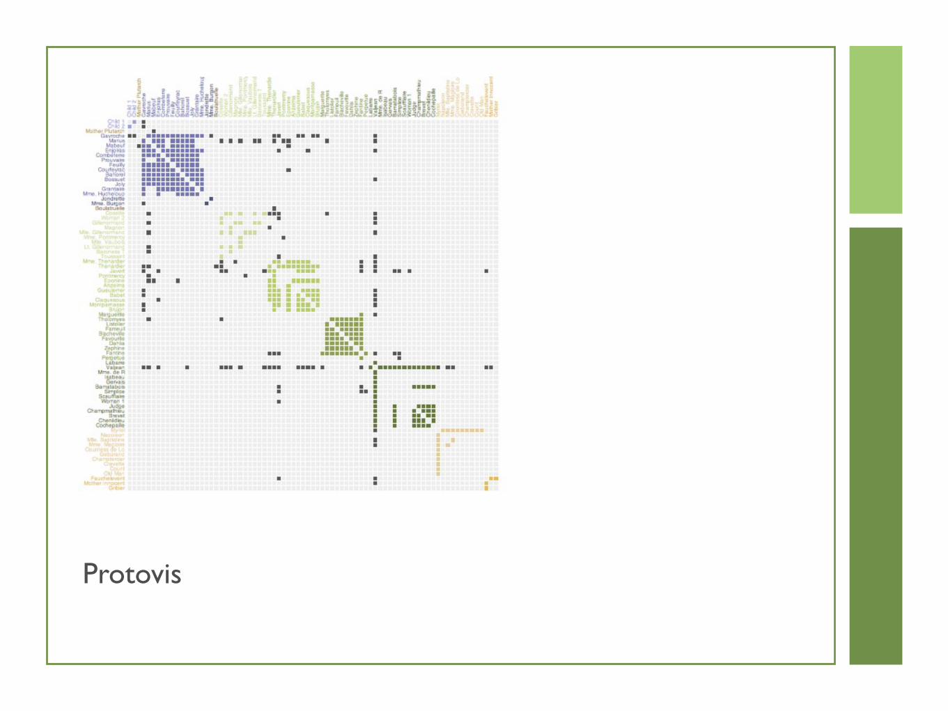
Protovis
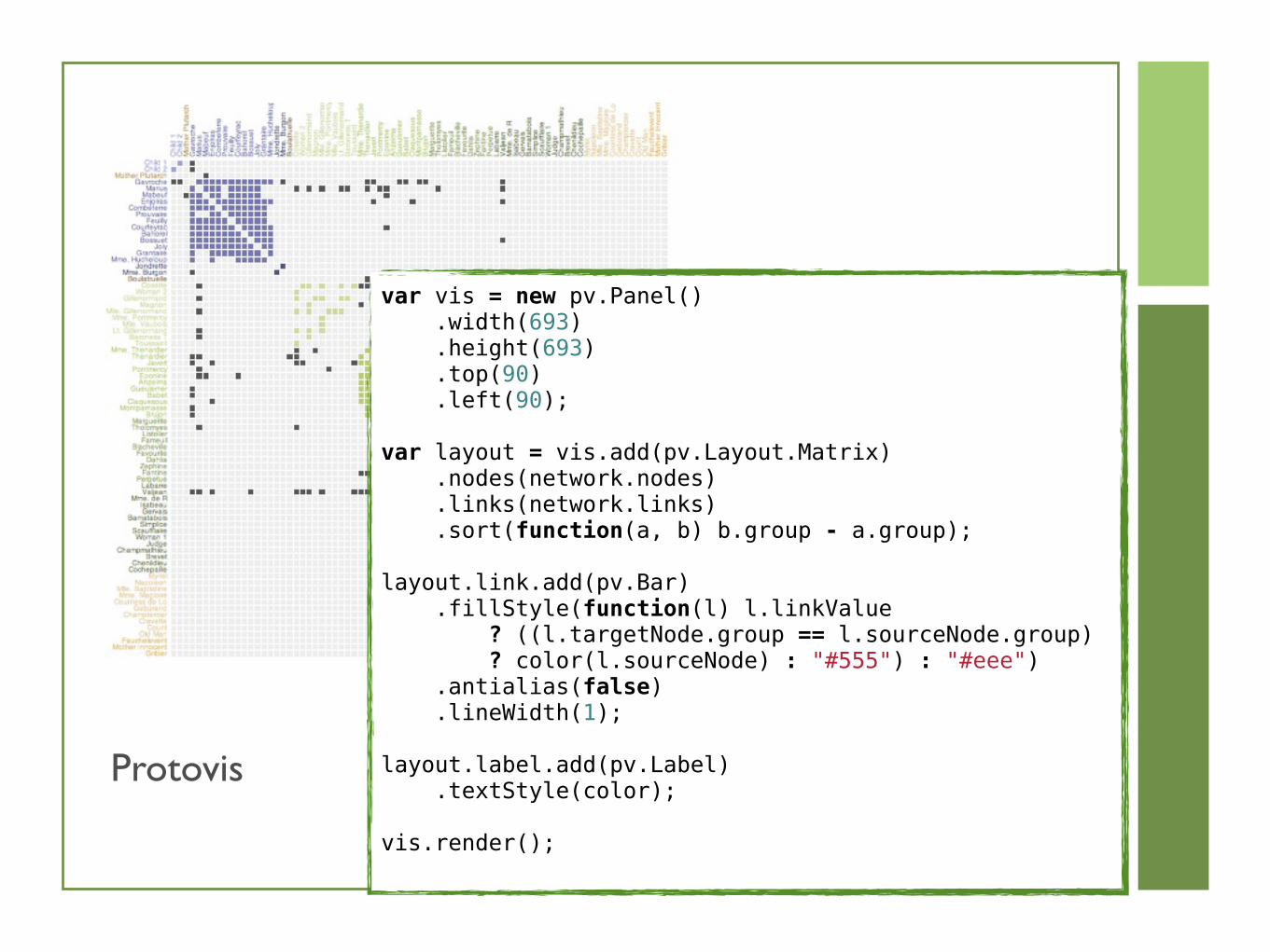
var vis = new pv.Panel() .width(693) .height(693) .top(90) .left(90);
var layout = vis.add(pv.Layout.Matrix) .nodes(network.nodes) .links(network.links) .sort(function(a, b) b.group - a.group);
layout.link.add(pv.Bar) .fillStyle(function(l) l.linkValue ? ((l.targetNode.group == l.sourceNode.group) ? color(l.sourceNode) : "#555") : "#eee") .antialias(false) .lineWidth(1);
layout.label.add(pv.Label) .textStyle(color);
vis.render();
Protovis
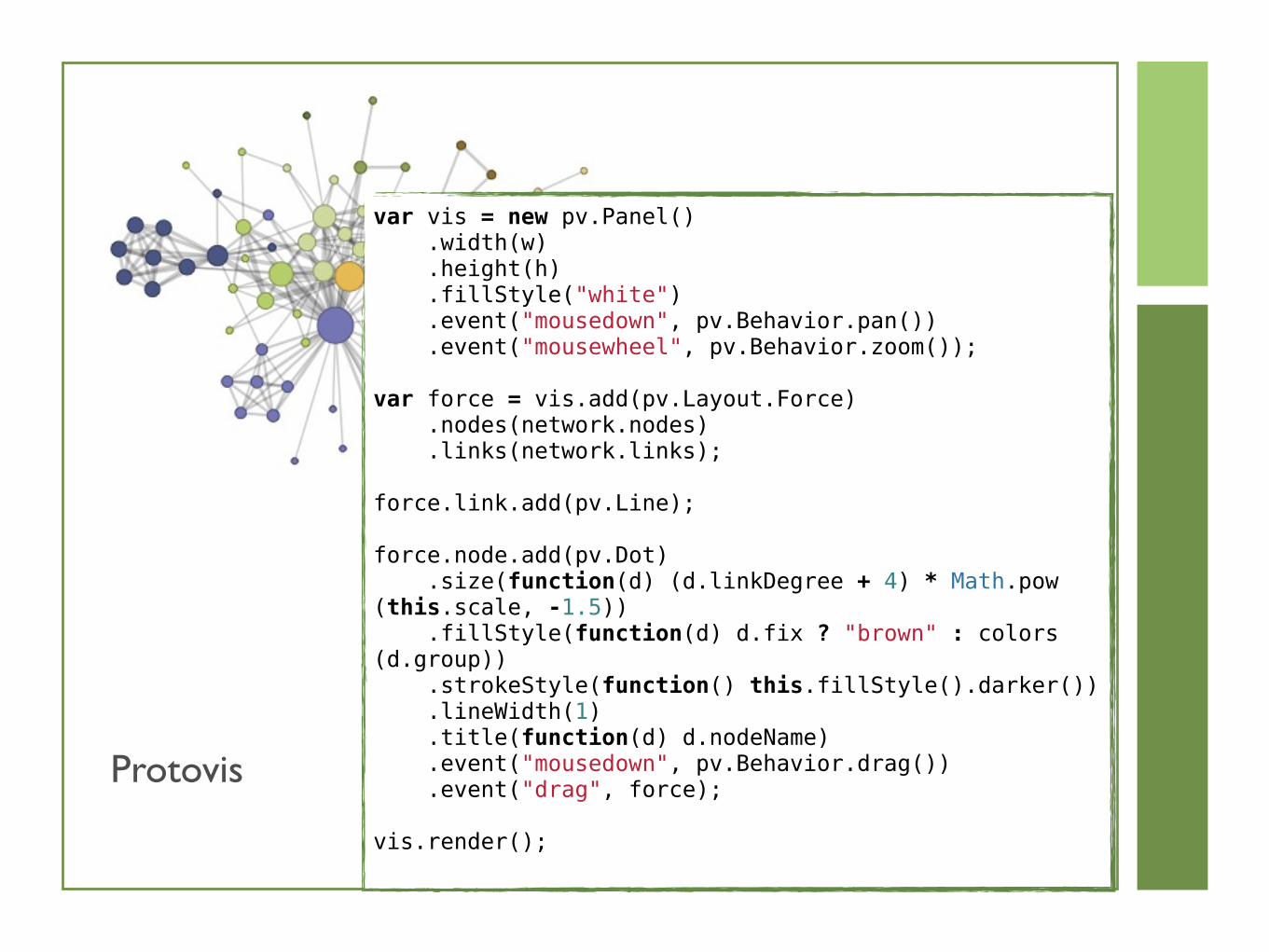
var vis = new pv.Panel() .width(w) .height(h) .fillStyle("white") .event("mousedown", pv.Behavior.pan()) .event("mousewheel", pv.Behavior.zoom());
var force = vis.add(pv.Layout.Force) .nodes(network.nodes) .links(network.links);
force.link.add(pv.Line);
force.node.add(pv.Dot) .size(function(d) (d.linkDegree + 4) * Math.pow(this.scale, -1.5)) .fillStyle(function(d) d.fix ? "brown" : colors(d.group)) .strokeStyle(function() this.fillStyle().darker()) .lineWidth(1) .title(function(d) d.nodeName) .event("mousedown", pv.Behavior.drag()) .event("drag", force);
vis.render();
Protovis

PageRank
Page Rank
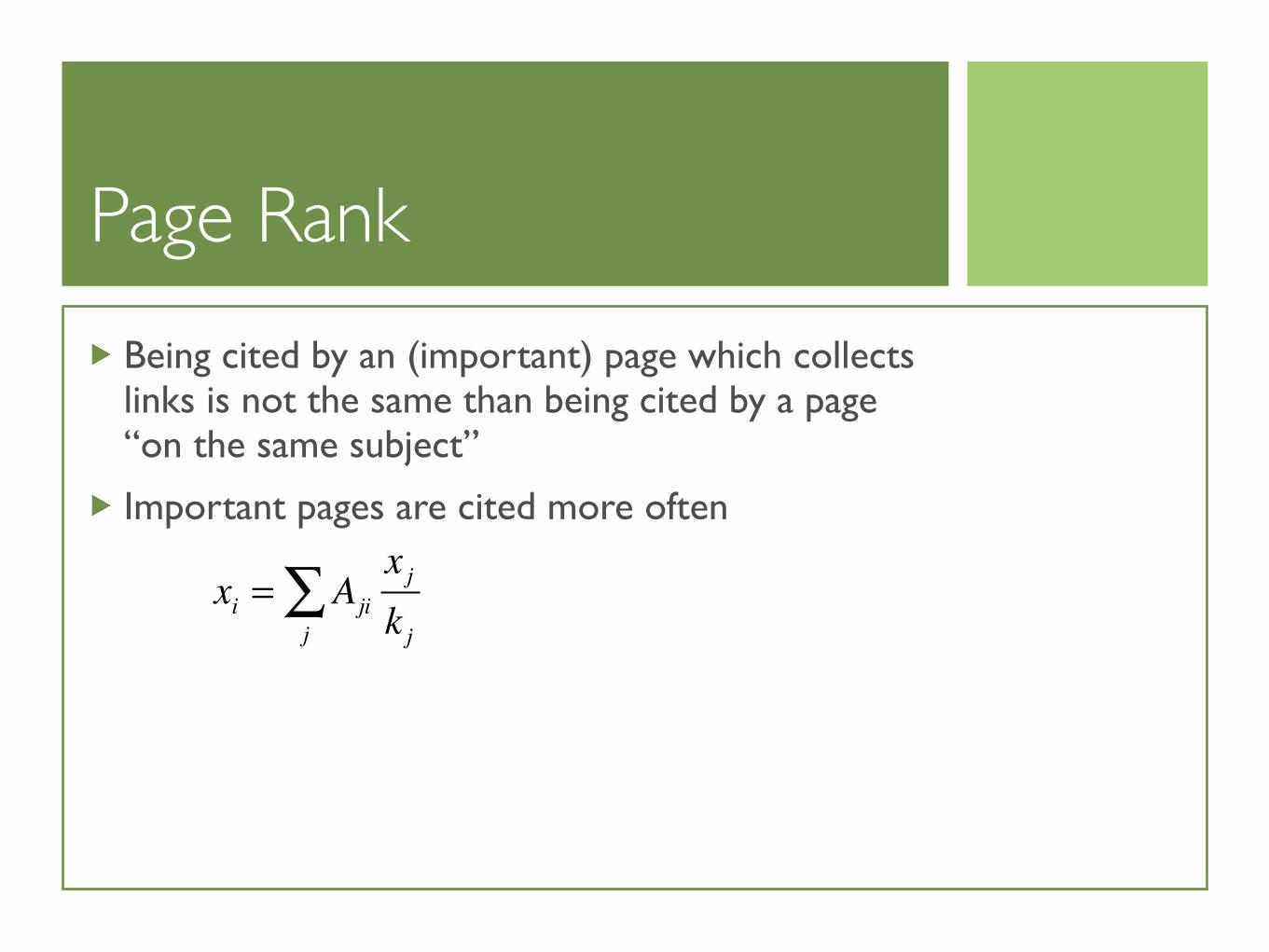
Being cited by an (important) page which collects links is not the same than being cited by a page “on the same subject”
Important pages are cited more often
xi = Aji
x jk jj
∑

Page Rank
In order to simplify the notation, we define the H matrix:
We can try to compute with successive approximations, like in with t→∞Each iteration takes O(n2) operations
the number of non-zero entries is O(n), which makes the computation O(n)
Convergence?
Hij = Aijk j−1
xH = xx(t) = x(0)Ht
Interpretation of Page Rank
Random Surfer
If time spent surfing approximates infinity, time spent on a given page is a measure of that page importance
Dangling Nodes
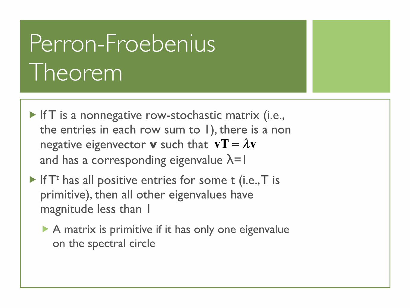
Perron-Froebenius Theorem
If T is a nonnegative row-stochastic matrix (i.e., the entries in each row sum to 1), there is a non negative eigenvector v such thatand has a corresponding eigenvalue λ=1
If Tt has all positive entries for some t (i.e., T is primitive), then all other eigenvalues have magnitude less than 1
A matrix is primitive if it has only one eigenvalue on the spectral circle
vT = λv
Primitivity Adjustment
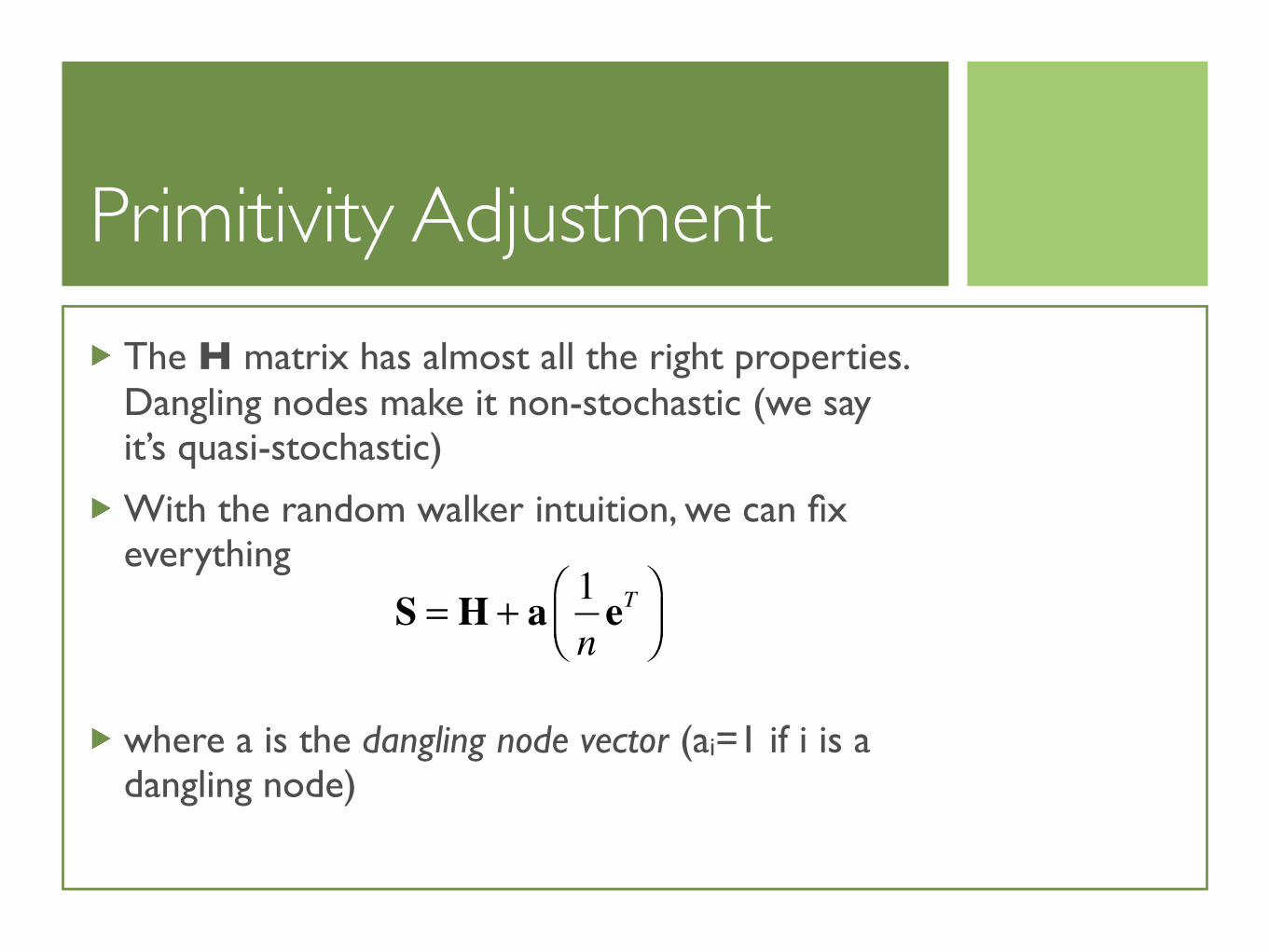
The H matrix has almost all the right properties. Dangling nodes make it non-stochastic (we say it’s quasi-stochastic)
With the random walker intuition, we can fix everything
where a is the dangling node vector (ai=1 if i is a dangling node)
S = H + a 1neT⎛
⎝⎜⎞⎠⎟

Markov Chains interpretation
S is the matrix of a Markov process
It is stochastic, irreducible (equivalent to say that the corresponding graph is strongly connected) and aperiodic
aperiodic + irreducible → primitive
From a mathematical point of view, everything is fine. However, we are implying that surfers never “jump” to entirely new pages
The Google Matrix
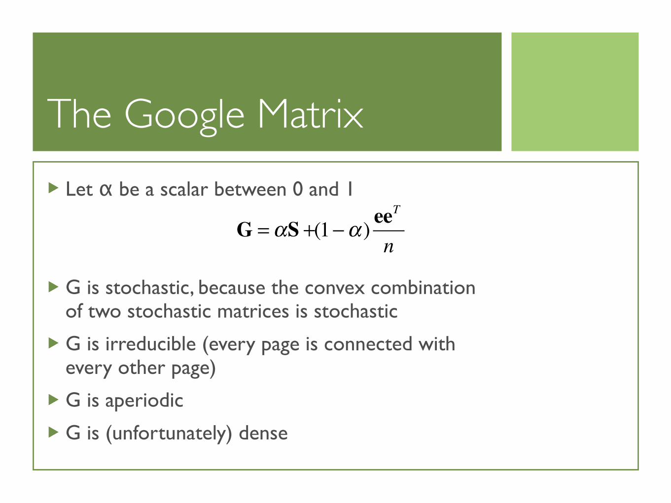
Let α be a scalar between 0 and 1
G is stochastic, because the convex combination of two stochastic matrices is stochastic
G is irreducible (every page is connected with every other page)
G is aperiodic
G is (unfortunately) dense
G = αS +(1−α ) eeT
n
Computing the PageRank
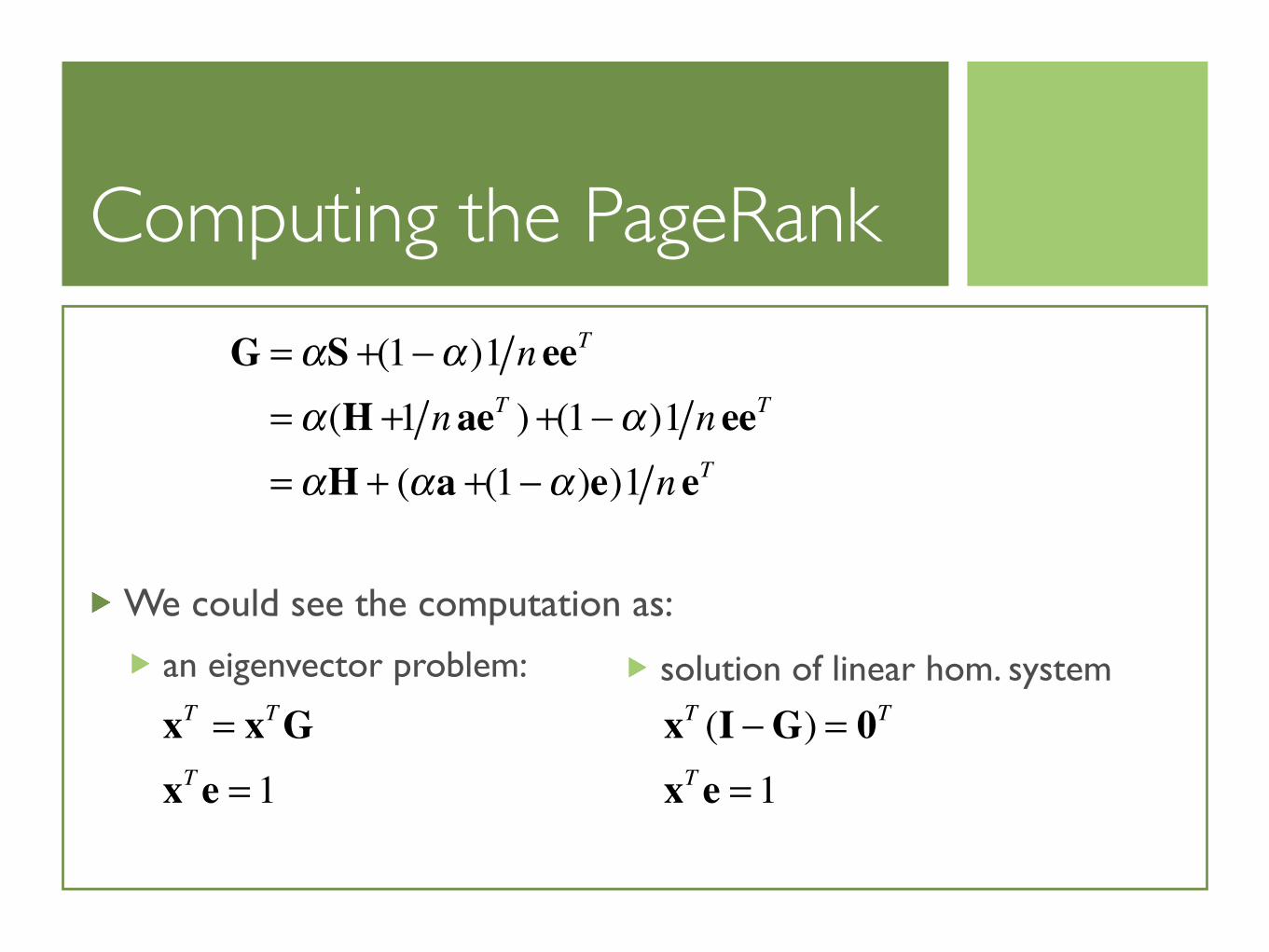
We could see the computation as:
an eigenvector problem:
G = αS +(1−α )1 n eeT
= α(H +1 naeT ) +(1−α )1 n eeT
= αH + (αa +(1−α )e)1 n eT
xT = xTGxT e = 1
solution of linear hom. system
xT (I −G) = 0T
xT e = 1
The Power-Method
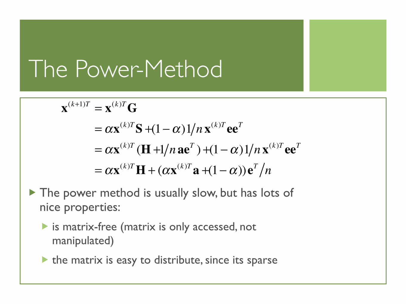
The power method is usually slow, but has lots of nice properties:
is matrix-free (matrix is only accessed, not manipulated)
the matrix is easy to distribute, since its sparse
x(k+1)T = x(k )TG= αx(k )TS +(1−α )1 nx(k )T eeT
= αx(k )T (H +1 naeT ) +(1−α )1 nx(k )T eeT
= αx(k )TH + (αx(k )Ta +(1−α ))eT n
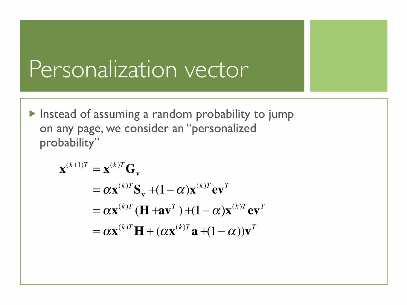
Personalization vector
Instead of assuming a random probability to jump on any page, we consider an “personalized probability”
x(k+1)T = x(k )TGv
= αx(k )TSv +(1−α )x(k )T evT
= αx(k )T (H +avT ) +(1−α )x(k )T evT
= αx(k )TH + (αx(k )Ta +(1−α ))vT

... in Python
Use networkx
nx.pagerank
nx.pagerank_numpy
nx.pagerank_scipy