Social Policy Evaluation and Research Unit - AUT · Social Policy Evaluation and Research Unit. ... Population movement during 5 years prior to 2013 ... economic and social science

Residential movement within New Zealand:Quantifying and characterising the transient populationNOVEMBER 2017

Social Policy Evaluation and Research Unit

Our purpose

The purpose of the Social Policy Evaluation and Research Unit (Superu) is to increase the use of evidence by people across the social sector so that they can make better decisions – about funding, policies or services – to improve the lives of New Zealanders and New Zealand’s communities, families and whānau.

SuperuPO Box 2839Wellington 6140

Telephone: 04 917 7040Email: [email protected]: superu.govt.nz

Follow us on Twitter: @nzfamilies Like us on Facebook: Social Policy Evaluation and Research Unit

ISBN 978-0-947489-98-4 (online) Learn more at: superu.govt.nz

New Zealand Work Research Institute, AUTLevel 5, 120 Mayoral Drive, Auckland Phone: +64 9 921 5056 Email: [email protected] Website: www.workresearch.aut.ac.nz

Report authors: Dr Nan Jiang, Professor Gail Pacheco and Dr Kabir Dasgupta.

For further information: [email protected]

AcknowledgementsWe are grateful to those organisations that provided us with assistance with their datasets, in particular the Auckland City Mission and Statistics New Zealand’s microdata team. An important thank you is also necessary for the external peer reviewer for this work, Professor Philip Morrison of Victoria University, for his valuable feedback and suggestions. Thank you also to Jason Timmins and John Wren for their additional feedback in shaping this research. Any errors or omissions remain the responsibility of the authors.

This report has been commissioned through the Ministerial Social Sector Research Fund, which is managed by Superu. The topic has been determined by the previous Minister of Finance, to meet policy concerns that might be addressed by expanding the available evidence. Superu is responsible for ensuring that appropriate research methods have been used, including peer review and quality assurance. Once released, all reports commissioned through the Fund are available on the Superu website superu.govt.nz and further information on the report can be provided by Superu.

Executive summary

The New Zealand Work Research Institute, at AUT, was commissioned by Superu to quantify the scale of transience in New Zealand and characterise the transient population, with a focus on those considered to be ‘vulnerable transient’.

Four percent of the New Zealand population are vulnerable transient

We found that 4 percent of the population can be categorised as ‘vulnerable transient’ (VT), and a further 1.3 percent can be categorised as ‘transient’ (T). We also found that close to half the VT population lived at an address for at least two short spells of less than 180 days each during our reference period. We measured transience over the period 1 August 2013 to 31 July 2016.

Receiving a welfare benefit was the most important characteristic associated with being vulnerable transient

We used a logistic regression to identify the key risk factors associated with being VT, for adults, youth and children separately. We found that being female, being Māori, being associated with a social welfare benefit, experiencing social housing, facing court charges (for adults and youth), having a Child, Youth and Family (CYF) event (for a child or young person), having a mental health event, and visiting a hospital emergency department (ED) were all associated with a substantial increase in odds of being in the VT group. The most important characteristic appears to be association with a social welfare benefit: in all three regressions the odds of being VT are more than 2.5 times greater for individuals associated with a benefit during the five years before our reference period than for those never involved in the benefit system over that same pre-reference period (holding all other factors constant).

It is also evident that, for most characteristics, the fact of having experienced that characteristic at all is much more important than the intensity of experience. For children, for example, being involved with a social welfare benefit was associated with odds of being 2.9 times more likely to be in the VT group, compared to those children not associated with a benefit spell. However, once a person is on a benefit, having additional weeks of association has no significant role in further increasing or decreasing the likelihood of being VT.

01

We found no standard definition for transience in prior literature

Existing studies have focused on residential movement, with negative outcomes often associated with frequent movement, as well as with movement to neighbourhoods with lower socio-economic status and higher deprivation. Past literature has linked high levels of residential movement with poorer outcomes in education, health and wellbeing.

We created the following subgroups: non-movers, low movement, medium movement, high movement (upward), transient, and vulnerable transient. We categorised people according to the number of moves reported in the three-year reference period, and according to whether a move was to a neighbourhood with a higher, lower or equal deprivation index score. For example, the VT category is defined as those who had at least three moves in the last three years, with at least one of the moves being to or within a high deprivation area (that is, an area with an deprivation index value of 8 to 10).

Address notification data was the best fit for measuring transience in New Zealand

We looked at the 2013 Census and the address notification data. Both are available in the Integrated Data Infrastructure (IDI) provided by Statistics New Zealand. The address notification data provides the best fit for this research as it allowed us to calculate the number of moves (within a specified timeframe), and it also provides more information for under five year olds, compared with the Census.

We used address information in the IDI over the most recent three years. We focused on New Zealand usual residents who lived throughout that period; this provided a population of approximately 3.8 million. Our analysis employed 11 datasets from the IDI, which were then merged on an individual basis, with the relevant population subgroups disaggregated by their type and frequency of residential movement. This provided comparable characteristics across different sub-populations, so that we could compare the transient and vulnerable transient subgroups with the rest of the population sample.


02

Contents

Executive summary 1

01 Introduction 6

1.1 Context 71.2 Priorliterature 7

02 Data 13

2.1 TheIntegratedDataInfrastructure 142.2 TheCensus 142.3 Addresstable 182.4 HowcanwecomparetheCensuswiththeaddresstable? 19

03 Definitions and populations of interest 22

3.1 Keyfactors=frequencyofmovement,socio-economicdirection,anddeprivation 23

3.2 Identifyingpopulationwithresidentialhistoryinthelastthreeyears 233.3 Removingnon-NZresidentsandthosewithmissinginformation 243.4 Definingnon-movers,movers,transients,andvulnerabletransients 25

04 Who is transient? 29

4.1 Whatisthesizeofthetransientandvulnerabletransientgroups? 304.2 Demographiccharacteristics 334.3 Movementpatterns 364.4 Socialwelfarebenefitsandservices 37 4.4.1 Associationswithsocialwelfarebenefit 37 4.4.2 Child,YouthandFamilyevents 39 4.4.3 Youthservices 414.5 Housinginformation 424.6 Justiceevents 444.7 Familyinformation 464.8 Healthcharacteristics 484.9 CasestudyofAucklandCityMission 49

03

05 Factors associated with vulnerable transience 51

5.1 Data 525.2 Method 545.3 Results 555.4 Futureresearch 58

Disclaimer 60

Appendix 61

References 62

List of FiguresFigure 1: Population movement during 5 years prior to 2013 Census 16Figure 2: Duration of residence under one year as at 2013 Census 17Figure 3: Comparison of census and address table – five years prior to Census date 20Figure 4: Comparison of census and address table – one year prior to Census date 21Figure 5: Defining movers and non-movers using the address table 27Figure 6: Age distribution for each population subgroup 34Figure 7: Ethnicity distribution for each population subgroup 35Figure 8: Proportion within each population subgroup on benefit 38Figure 9: Average time within each population subgroup on benefit 38Figure 10: Proportion within each population subgroup that were CYF clients 40Figure 11: Average number of CYF events in each time period, by population subgroups 40Figure 12: Proportion within each subgroup living in social housing 43Figure 13: Proportion within each population subgroup with justice events 44Figure 14: Proportion within each population subgroup receiving working for families 47


04

List of Tables

Table 1: Typology of the definitions of transience 9Table 2: Census questions related to population movements 15Table 3: Comparison of movement between census and address table 19Table 4: Size of key population groups 31Table 5: Duration of stay – transient groups 31Table 6: Size of transient groups – sensitivity results 32Table 7: Movement patterns for T and VT 36Table 8: Youth service interventions by population subgroups 41Table 9: Average number of months for social housing users 43Table 10: Descriptive information for individuals with court charges 45Table 11: Relationship events for each population subgroup 47Table 12: Health events by population subgroups 49Table 13: ACM characteristics by population subgroups 50Table 14: Definitions for explanatory variables in logistic regression analysis 53Table 15: Logistic regression results for belonging in the VT group 56

05

01Introduction


06

1.1_ Context

The Social Policy Evaluation and Research Unit (Superu) manages a Ministerial fund for social sector research. The purpose of this fund is to help inform policy thinking and decision making. As a further project for this fund, Government Ministers asked Superu to commission new research to answer the following questions:

• What is the scale of transience in New Zealand?

• What are the characteristics of transient populations in New Zealand, and of ‘vulnerable’ transient populations in particular?

Superu commissioned the New Zealand Work Research Institute (NZWRI) of Auckland University of Technology (AUT) to conduct this research and analysis. We have used Statistics New Zealand’s Integrated Data Infrastructure (IDI) to build workable definitions of ‘transience’ and ‘vulnerable transience’, using the three most recent years of data to answer the research questions stated above.

1.2_ Prior literature

What is transience?

In general terms, ‘transient’ means temporary or short-lived, but unfortunately there is no single definition of ‘transient’ or ‘transience’ in research or social policy circles. Health, economic and social science literature tends to use the term ‘residential mobility’ rather than ‘transience’, because home or place of residence is the key mode of connection to a neighbourhood, a community, social support services, and other forms of social capital.1

Superu currently defines transience broadly, as:

“Repeated disruption of key social support mechanisms (including residence) which is associated with negative impacts on social, health, education, and/or employment outcomes.”

1 Note that this is not the case for homeless individuals.

07

Components of this definition may vary depending on the population group of interest and the perspective taken. For example, if we are focusing on children, and using an educational perspective, ‘repeated disruption’ may mean changing schools a certain number of times within a year and/or at times other than the normal start of the school year (for example, see Kariuki et al. 1999; Strand 2000). Alternatively, if we are focusing on families or households, and using an economic perspective, ‘repeated disruption’ may mean moving residential address at least once a year (for example, see Morton et al. 2014).

Understanding the driving forces and consequences of transience requires differentiating between different types of moves. For instance, the motivation and outcomes associated with moving to a better home in a better neighbourhood are likely to be different from those associated with moving frequently between inadequate housing. Identifying vulnerable populations who are more likely to experience disadvantaging or downward moves (ie moves to neighbourhoods with lower socio-economic status) is important for developing appropriate policies to mitigate adverse outcomes.

Table 1 summarises the typology of definitions in the literature, with a focus on residential movements.


08

TABLE

01Typology of the

definitions of transience

Source: Authors’ compilation.

Typology Nature of move Definition

Residential movement in general

Advantaging moves

Moves that are voluntary, timely and to better homes, better neighbourhoods, or better schools (Lupton 2016)

Disadvantaging moves

Involuntary or frequent moves, or moves to worse housing or worse neighbourhoods or schools (Lupton 2016)

Residential movement by deprivation

Upward movement

Moves from more deprived neighbourhoods to less deprived neighbourhoods (Exeter et al. 2015)

Downward movement

Moves from less deprived neighbourhoods to more deprived neighbourhoods (Exeter et al. 2015)

Sideways movement

Moves within or between neighbourhoods with the same level of deprivation (Exeter et al. 2015)

Residential movement by frequency

Stayers This includes people who do not move, whether they are living in high, medium or low deprivation neighbourhoods (Exeter et al. 2015).

High This includes people who move frequently during a given period. The number of moves and the time period depend on the definition used.

Medium This includes people who move, but not frequently (usually only once during a given period).

Residential movement by distance

International move

This includes people who move to or from another country during a given period (Statistics NZ 2006).

Inter-regional move

This includes people who move between regions within NZ during a given period (Statistics NZ 2006).

Intra-regional move

This includes people who move within a region during a given period (Statistics NZ 2006).

Local move This can be defined by moves within smaller geo-political units, or by distance (e.g. ≤50km, ≤5km) (see Morton et al. 2014).

Transience unrelated to residential move

Changing school This includes people who change school frequently (for reasons unrelated to progression) without moving residential address. This may include those who change because of school preference, but may also include children in foster care who change schools because of special needs or disciplinary issues (Bull & Gilbert 2007).

Changing health provider

This includes people who change health provider frequently without moving residential address. Reasons for this may include financial difficulties or other reasons unrelated to any measure of hardship.

09

As evident from Table 1, ‘transience’ and ‘residential movement’ in particular are variably defined. These concepts have been quantified by researchers, using descriptors such as distance moved, reason for shift, frequency, attributes of neighbourhoods moved to or from, and time since residential change (Jelleyman & Spencer 2008). For the purposes of the following analysis, we focus on movement by deprivation and by frequency (see Section 2.5 for more details) as core elements of our definition of transience, and then characterise the populations of interest by a range of factors, including movements defined by distance (more specifically, intra – versus inter-regional patterns).

Why is it important to understand the scale of transience?

There are a number of studies that link frequent residential movement with poorer outcomes for the affected individuals and their families. These include impacts on educational outcomes for children (Hutchings et al. 2013; Schwartz et al. 2015; Bull & Gilbert 2007; Neighbour 2000; ERO 1997), and health outcomes (Turnstall et al. 2012).

Frequent residential moves, especially involuntary ones, can also worsen physical and mental wellbeing and future human capital (Heller 1982; Stokols et al. 1983; Magdol 2002; Schafft 2006). As a consequence, transience is likely to be related to poor labour market outcomes and even to a lack of employment opportunities (Currie & Madrian 1999). Additionally, changes in neighbourhood qualities and social characteristics associated with residential movement may also influence labour market activities and employment outcomes (Weinberg et al. 2004; Bayer et al. 2008; Oishi 2010). Those kinds of relationships highlight the complexity of transience, which is an area where the same factors can be both determinants and outcomes of frequent moves.

Many of the relevant studies also acknowledge that the likely reasons for strong associations between residential movement and poorer outcomes can potentially be the drivers behind a move, rather than simply the move itself. The drivers identified tend to fall into the following life event classifications: (1) relationship events such as separation, divorce and re-partnering; (2) economic events, usually related to the labour market; (3) housing events, usually involuntary, such as foreclosure or eviction; (4) health events, which can be both a driver and an outcome; and (5) justice events, such as being a victim or perpetrator of crime, or imprisonment of a family member.

A better understanding of the scale and types of residential movements occurring across a population is important for developing policy on housing and on security and safety for families, as well as neighbourhood design and development. In the New Zealand context, there are a number of policy areas where a better understanding of residential movement and transience is imperative. These include service transience (including school absenteeism); access to and participation in early childhood education; housing quality; child vulnerability and resilience; and support for families that require multiple service interventions.


10

What is the New Zealand evidence on population movements?

Evidence on the scale of residential movements in New Zealand is scant at best. The few studies in this space also show how population movements have been captured over time based on the type of data available. For example, Keown (1971) acknowledged the lack of population movement data in New Zealand by pointing out potential sources of proxy information used by researchers, included city directories (Goldstein 1958) and electoral rolls (Johnston 1967). Heenan (1979) contributed to the first comprehensive book in New Zealand in the field of population study. Heenan’s chapter was on internal migration patterns: he used 1971 Census data to characterise internal migration trends by age and gender profiles. He also emphasised the rural versus urban trends in migration,2 and the perceived drift north of the country’s population.

Following these early studies, the Census became the primary source of information on movement and on duration of residence – see for instance Statistics NZ reports based on the Census (2001, 2006, 2013). At the aggregate level, based on the last Census wave (2013), close to half the usually resident population aged five years and over (49.4%) reported living at the same address as in 2008. This was an increase from the 2006 Census figure of 41.1 percent. This was also a reversal of a general decline in the proportion of people living at the same address as five years earlier, a trend that was evident from the 1991 Census through to 2006. This apparent drop in population movements mirrors trends reported in the international literature. For example, there have been similar findings in the UK (Champion & Shuttleworth 2015a, 2015b), and the US (Cooke 2011, 2013; Molloy, Smith & Wozniak 2011).

Another study using Census information to track residential movement was by Morrison and Nissen (2010). The authors used the 2001 and 2006 Census waves and linked them with information from the NZ Deprivation index to produce inter-decile mobility matrices. They found for instance that nearly three-quarters of movers changed their position in relation to their neighbourhood’s Deprivation Index score over the five-year period between the Census waves. They also observed an inverse relationship between the neighbourhood decile and upward movement. When the analysis is broken down into subgroups, results indicate that the likelihood of movers remaining in their decile of origin rises with the original deprivation level, but at a declining rate with age.3

2 Results pointed to the majority of internal migration being within, between, or to and from major urban areas.3 Substantial ethnic differences were also apparent.

11

Other recent sources of population movement data include the Survey of Dynamics and Motivation for Migration in New Zealand (DMM), and cohort studies such as the Growing Up panel (Morton et al. 2014). The DMM survey was undertaken by Statistics NZ in March 2007 to investigate what motivates people to move (within, as well as to and from, New Zealand), and what motivates people to stay where they are. The survey found that approximately a quarter of the survey population had moved at least once during the two years before the March 2007 quarter. Morrison and Clark (2011) used the survey to illustrate that only a minority of migrants move between local labour markets for employment reasons. In a follow-up study, Clark and Morrison (2012) used the survey again, to show that movement by those leaving the very deprived areas was less likely to be an upgrade in neighbourhood; this was particularly evident for those reporting low incomes. While the DMM survey was a one-off by Statistics NZ, the Growing Up study is collecting ongoing information on a range of topics for a birth cohort born across the wider Auckland region in 2009. This includes information on residential movements. For instance, Morton et al. (2014) reported that 45.3% of their sample had moved at least once between the birth of the child and the child’s second birthday.

As evident from the examples above, a determining factor in how residential movement has been measured in New Zealand has often been the limitations of the available data. Section 2 provides details on the potential sources of current data in this space and assesses their usefulness for building a comprehensive portrait of residential movements in New Zealand.


12

02Data

13

2.1_ The Integrated Data Infrastructure

This research uses information from Statistics New Zealand’s Integrated Data Infrastructure (IDI).4 The IDI is a large research database containing microdata about individuals and households. It provides a wealth of administrative data from a range of government agencies. It also includes numerous Statistics NZ surveys, as well as data derived from non-government agencies, such as the Auckland City Mission.

Every individual in the IDI is assigned a unique identifier (snz_uid) that permits linkages across datasets and different tables, and also allows the researcher to take a longitudinal perspective when appropriate. This will enable us in the analysis section to look at the characteristics of individuals during the relevant reference period, as well as their characteristics prior to the reference period.

The two potential sources of data within the IDI that relate to population movements are the 2013 Census and the address table. These two datasets are described in Sections 2.2 and 2.3, along with appropriate caveats for the purposes of this research. After comparing the two datasets, we weigh up the advantages and disadvantages of each based on the scope and aims of this research, in order to decide which data source has the best fit for this research.

2.2_ The Census

Population movement information available in the Census

The most recent Census of population and dwellings (2013) is available in unit record form in the IDI.5 The main aim of this dataset is to provide a snapshot of the New Zealand population (both in terms of individuals and dwellings) at a point in time. The target population of interest with this self-reported survey is individuals in New Zealand on Census night who are usually resident in New Zealand. Census night was Tuesday, 5 March 2013.

There are two questions in the Census that provide information related to population movements, and these are detailed in Table 2.

4 More information on the IDI can be found at Statistics NZ (2017).5 Note that no prior census waves are currently available in the IDI.


14

TABLE

02Census questions

related to population

movements

Residential move within 5 years Duration of residence

Question:‘Where did you usually live 5 years ago, on 5 March 2008?’

Response codes:1 Same as usual residence2 Elsewhere in NZ3 Not born 5 years ago4 Overseas5 No fixed address 5 years ago77 Response unidentifiable99 Not stated

Question:‘How long have you lived at the address you gave in Question 5?’6

Response codes:Integer values 0–98 representing the number of years a person lived in their current address777 Response unidentifiable999 Not stated

Notes: Sourced from the 2013 Census Data Dictionary.

Who has moved within the last five years?6

For the first question in Table 2, grouping responses 2, 4 and 5 provides an indication of the level of movement across the population within a five-year window. This information is shown in Figure 1, where it is evident that nearly half of the population (46.6%)7 had moved (at least once) in the five years preceding the Census night. In particular, the adult population aged 20 to 40 experienced higher levels of movement than other age groups, with those aged 25 to 29 being the group most likely to have moved (79.9%).

Young adults are more susceptible to labour market uncertainties (such as changes in employment opportunities with changing economic conditions) and are more likely to undertake labour market risks (that is, to take on new jobs). These factors often contribute to their high rates of residential movement relative to other age groups.

Respondents aged 75 to 79 were the group least likely to have moved within the five-year window (26.6%).

It is useful to note that the age-specific movement patterns in the period 2008–2013 mirror those from the 2006 Census (Statistics NZ 2006). The most mobile group in that earlier Census was also 25 to 29 year olds (83.9%), and the least mobile group was also 75 to 79 year olds.

6 The ‘address you gave in Question 5’ is the individual’s current address.7 In Australia, by comparison, 41.7 percent of residents had moved in the five years prior to the 2011 Census

(Australian Bureau of Statistics 2012).

15

Figure 1 _ Population movement during 5 years prior to 2013 Census

80

60

40

20

0

Perc

enta

ge

0-4

year

s

5-9

year

s

10-14

yea

rs

15-19

yea

rs

20-2

4 ye

ars

25-2

9 ye

ars

30-3

4 ye

ars

35-3

9 ye

ars

40-4

4 ye

ars

45-4

9 ye

ars

50-5

4 ye

ars

55-5

9 ye

ars

60-6

4 ye

ars

65-6

9 ye

ars

70-7

4 ye

ars

75-7

9 ye

ars

80-8

4 ye

ars

85 y

ears

and

ove

r

All a

ges

79.9

57.6

49.151.8

70.2

76.0

65.0

53.8

44.4

38.034.5

31.7 29.827.2 26.6 27.7

34.8

46.6

0.0

Note: Data sourced from 2013 Census.

Who has moved within the last year?

The second question in Table 2 – which asks how long the person has lived at their current address – is often used not only to obtain data on duration of residence at the current address, but also to indicate a residential move within the last year. Individuals who respond to that question with a value of ‘0’ signal that they have lived at their current address for less than a year as of the Census date. Figure 2 indicates that those aged 20 to 24 had the highest propensity to have moved within that timeframe (45.1%), while those aged 70 to 79 were the least likely (7.4%). Overall, 22.1% reported that they had lived at their current residential address for less than a year prior to the 2013 Census.

A comparison of the information in Figures 1 and 2 with prior Census waves indicates that the aggregate level of population movement has declined. For instance, the proportion of the usually resident population that had a duration of residence of under a year at their current address on Census night 2013 was 22.1%, while the comparable figures in the 2006 and 2001 Censuses were 24.8% and 24.2% respectively. Additionally, in both the 2006 and 2001 Censuses, more than half the population had changed their usual residence at least once in the previous five years (57.7% for 2006, and 55.4% for 2001), and the comparable figure was substantially lower in 2013, at 46.6%.


16

Figure 2 _ Duration of residence under one year as at 2013 Census

50

40

30

20

10

0

Perc

enta

ge

0-4

year

s

5-9

year

s

10-14

yea

rs

15-19

yea

rs

20-2

4 ye

ars

25-2

9 ye

ars

30-3

4 ye

ars

35-3

9 ye

ars

40-4

4 ye

ars

45-4

9 ye

ars

50-5

4 ye

ars

55-5

9 ye

ars

60-6

4 ye

ars

65-6

9 ye

ars

70-7

4 ye

ars

75-7

9 ye

ars

80-8

4 ye

ars

85 y

ears

and

ove

r

All a

ges

41.7

20.517.3

27.5

45.1

31.9

23.8

18.6

14.912.7

11.29.7 8.6 7.4 7.4 7.9

10.6

22.1

42.4

Note: Data sourced from 2013 Census.

What information does the Census not provide?

A potential disadvantage is that the only Census questions related to population movement lack detail on the number of moves within a specified timeframe, as well as on the duration of residence and neighbourhood qualities at previous addresses. Data on frequency of movement, as well as on deprivation and the socio-economic direction of movement, are imperative for understanding transience; the Census therefore appears unlikely to be a suitable data source for the purpose of this study.

The second disadvantage of the Census questions is the dearth of information related to young children. For instance, the first question in Table 2 produces no information for individuals under the age of five. Further, for children aged under 12 months, the second question in Table 2 (on duration of residence at the current address) doesn’t allow us to distinguish between those who moved in the last year (and therefore have been at their address for less than a year) and those who have lived at the same address since their birth. Given that 39% of the 0 to 4 age category is made up of children under 12 months, this is the likely reason for an apparently high proportion of this group (42.4%) living at their address for less than a year. We must therefore treat the estimates from this group with caution, and avoid inferring likelihood of population movement from this information.

A final disadvantage of the Census is that it could be subject to recall bias due to the self-reported nature of the data collected. It is however important to recognise that there is no evidence available to confirm the existence of the bias or to indicate the likelihood of its potential influence on residential movement estimates in the Census.

17

2.3_ Address table

Population movement information available in the address table

The Integrated Data Infrastructure (IDI) combines information from a number of sources to produce an efficient geospatial resource for users. Address records are collected from eight sources (spanning six agencies): Ministry of Health Primary Health Organisation registers; Ministry of Health National Health Index records; Ministry of Social Development residential; Ministry of Social Development postal addresses; Ministry of Education records; ACC client addresses; Inland Revenue (IR) tax registration addresses; and the 2013 Census.

All of the address information is geocoded by Statistics NZ and prioritised (using a simple set of business rules) to limit the address notification table to a best-guess list of residential addresses for each snz_uid (that is, each individual). The order of priority is provided by the list of sources above, indicating that an address on the Ministry of Health Primary Health Organisation register will take priority over other sources, and that the next source of priority is an address recorded with the Ministry of Health National Health Index. If no address exists for that source, Statistics NZ moves down the list until reaching the lowest ranked address source, which is the 2013 Census.

The result is a chronological record of the (prioritised) usual residential address for individuals in the IDI.

What information does the address table not provide?

It is important to note that available address information is ‘observational’: that is, a record of an address only occurs when an individual notifies an agency of a change in address.8 The date of notification is therefore unlikely to be the actual date of the residential move. However, as long as there is not a substantial lag between the moving date and the address notification, this lack of information should not impede our research exercise.

A second disadvantage of the address table is that some sources of information may have missing data and/or other quality issues. This potential bias affecting estimates of population movement is likely to be more prevalent for individuals not in our focus (that is, not transient). This is because transient individuals probably have more interactions with the six source agencies for the IDI address table, and are therefore more likely to have their address changes recorded, and less likely to have missing information. This is especially true for agencies such as the Ministry of Health and the Ministry of Social Development, who require address information from their clients.

8 The address table will therefore not provide full coverage in some circumstances. For instance, it will not include individuals who move from the house of one friend to that of another (and therefore may be technically transient), and do not have any contact with government agencies that will record their address movements.


18

2.4_ How can we compare the Census with the address table?

To construct a comparison between the 2013 Census and the address table, we limit our population of interest from the address table to those with Census records. This encompassed 93.3% of the population covered in the Census wave, which is 4.06 million individuals.

The first point of comparison relates to the first question in Table 2 (Section 2.2) – that is, whether individuals in the Census reported that they had moved within the last five years, and whether the address table also reveals these individuals as movers within the period 2008 to 2013.

Table 3 provides this comparison in a dichotomous fashion. It shows that there is a 70.43% match rate for non-movers, while the match rate for movers is 87.82% (see the shaded cells in Table 3).

TABLE

03Comparison

of movement between Census

and address table

Address table Total (m)

Census

Non-mover Mover

Non-mover 1.58 0.66 2.24

(70.43%) (29.57%)

Mover 0.22 1.59 1.81

(12.18%) (87.82%)

Total (m) 1.80 2.26 4.06

Note: Comparison is based on five years prior to Census date. Percentages in parenthesis are relative to the row total. Sample sizes are in millions of individuals and rounded to 2 decimal places. Matched population between Census 2013 and the address table in the IDI.

Figure 3 takes the comparison a step further to illustrate the additional information provided by the address table (beyond a binary response of move / didn’t move) in terms of the number of moves within that timeframe. The solid line represents individuals who reported in the Census that they had moved in the previous five years. This is 1.81 million individuals. Of this group (as also shown in Table 3), just over 12% are identified as non-movers based on the address table information. The dashed line corresponds to individuals who reported in the Census that they had not moved in the previous five years. This is 2.24 million individuals.

19

Figure 3 _ Comparison of Census and address table – five years prior to Census date

80

60

40

20

0

0 2 4 6 8 10+

Movers in Census2013 Non-movers in Census2013

Prop

ortio

n of

mat

ched

pop

ulat

ion

Number of moves

Source: Matched population between Census 2013 and the address table in the IDI. Number of moves is based on information from the address table.

When focusing on the second question in Table 2 (Section 2.2), we can compare (1) individuals’ reporting in the Census that they have been at their current residence for less than a year with (2) movement patterns in the address table during that one-year timeframe.

Figure 4 presents this comparison and shows that of those reporting that they had been at their residence less than a year (the solid line), 21% of these individuals do not have an address notification change within the address table in the IDI, 57% have one address change, and the remainder of this sample have multiple address change notifications. Of those who reported being at their current address for at least one year (the dashed line), 80% of this group were also classified as non-movers according to the address table.


20

Figure 4 _ Comparison of Census and address table – one year prior to Census date

80

60

40

20

0

Prop

ortio

n of

mat

ched

pop

ulat

ion

0 1 2 3 4 5+

Duration at current residence less than a year

Duration at current residence equal to or more than a year

Number of moves

Source: Matched population between Census 2013 and the address table in the IDI. Number of moves is based on information from the address table.

Regardless of whether we focus on movers or non-movers, why are the match rates in Figures 3 and 4 not 100%? The exact causes of the differences is unknown. Based on the information provided in Sections 2.2 and 2.3, we know that Census estimates may be affected by recall bias, and lack information on young children (especially under five year olds for Figure 3). Address table estimates may have their own quality issues, as well as missing information for some of the data sources from which the address table is generated.

For the purposes of our research exercise of identifying the transient population, we expect transient individuals will have more interactions with service provision agencies (such as the Ministries of Health and Social Development) and will therefore be less likely to be affected by the sources of bias that affect address table estimates.

Most importantly, as shown in Figures 3 and 4, the address table provides more detailed information on the number of moves, which the Census cannot help with, and this frequency information is imperative for building a workable definition of transience.

In the next section we therefore focus solely on the address table information from the IDI,9 and define (and subsequently quantify) our relevant populations of interest.

9 Future research could delve into other aspects of the Census and address table data that are not of primary rele-vance to this research exercise. For example, there could be further tests on quality aspects of the address table for particular population subgroups, as well as research to develop a better understanding of whether recall bias is prevalent in the Census.

21

03Definitions and populations of interest


22

3.1_ Key factors = frequency of movement, socio-economic direction, and deprivation

The aim of this study is to quantify New Zealand’s transient population. Given the lack of specific literature defining transience, we have relied on the small number of prior studies on residential movement. As shown in Table 1 (in Section 1.2), there are three aspects of movement that surface regularly in discussions of residential movement and future outcomes. These are the frequency of movement, the socio-economic characteristics of neighbourhoods, and the socio-economic direction of the move. The first of these – frequency – is commonly used as a way of measuring the dose-effect of residential movement, while the second factor – socio-economic status of neighbourhoods – is often a proxy for the potential socio-economic status of the individual and their likely vulnerability. In relation to the socio-economic direction of movement, upward mobility is often associated with good outcomes and tends to represent positive change, while downward mobility can be associated with mixed outcomes, and depends on the drivers of the move (Exeter et al. 2015; Lupton 2016).

Focusing on those three factors, we can build a definition for transience using information from the address table in the IDI. The following subsections (3.2 to 3.4) explain in detail the construction of our data sample and, further, the mechanisms and rules we used to partition this sample into populations of interest. We divide our population into non-movers, low movement, medium movement, high movement (upward), transient, and vulnerable transient.10 The rules governing these divisions are based on frequency of movement, deprivation (as a proxy for the socio-economic status of neighbourhoods), and socio-economic direction of the move.

3.2_ Identifying population with residential history in the last three years

We begin with the full list of prioritised address notifications in the IDI address table, which includes information for individuals who have a residential address record in New Zealand since 2000, up to 31 July 2016. The address table is described in Section 2.3.11 This dataset is essentially a prioritised list of addresses; it currently has more than 27 million address records.

10 Note that ‘upward’ and ‘downward’ refer to the direction of movement in relation to the Deprivation Index (as shown in Figure 5).

11 See http://stats.govt.nz/browse_for_stats/snapshots-of-nz/integrated-data-infrastructure/idi-data.aspx#geo-graphic for a description of the address notification table in the ‘Geographic’ section.

23

We limit our focus to the last three years of data – that is, 1 August 2013 to 31 July 2016. There are three reasons for this timeframe: (1) it is after the 2011 Christchurch earthquake, which created a greater than usual increase in involuntary population movements at that time, particularly in the South Island; (2) this timeframe provides the most up-to-date data, allowing for policy to be developed on the basis of the latest information; and (3) if we lengthen our timeframe to more than three years, we will lose more observations, as we require individuals to be present during the entire period under study.

Based on the three-year window, our sample is limited to approximately 11.93 million address records, which are associated with 8.29 million unique individuals. Where an individual seems to have the same address in two consecutive address spells, Statistics NZ has recommended collating these spells; this reduces our data sample to 11.88 million address events.12

3.3_ Removing non-NZ residents and those with missing information

Starting with the sample of 8.29 million individuals identified above, we dropped all individuals who do not appear to have been New Zealand usual residents during the entire reference period. This involved a number of cuts to our sample.

The first was the removal of 633,72613 individuals with death records (using data from the Department of Internal Affairs – DIA). This left us with 7.66 million unique individuals.

Next, we removed those who do not have New Zealand citizenship or residence, using the ‘immigration visa application decisions’ table. We eliminated those immigration clients whose most recent visa application belonged to the ‘temporary’ category, or whose most recent application was for ‘residence’ but was not granted before 1 August 2013. This left us with a sample of 6.19 million unique individuals.

We further dropped 1.41 million individuals who left New Zealand before 1 August 2013 and never came back (using the ‘border movements’ table), and another 530,796 people who spent less than 50% of their time in New Zealand during the reference period. This left us with 4.24 million unique individuals.

We then removed 79,263 individuals who do not have a death record with DIA but who had a decease date according to Ministry of Health data, and 305,208 babies who were born after the start of our reference period (1 August 2013).

12 45,819 address records share the same address ID as the individual’s previous address episode.13 All sample sizes in this study are random rounded to base 3, due to Statistics NZ requirements for

confidentiality assurance.


24

Finally, as construction of our population subgroups requires information on how addresses score on the Deprivation Index, our final step in constructing our sample was to drop an additional 1,461 individuals whose address records are missing that deprivation information.

The final sample for our analysis equates to 3,857,433 unique New Zealand citizens or residents who lived through the entire reference period (1 August 2013 to 31 July 2016).

3.4_ Defining non-movers, movers, transients, and vulnerable transients

We next partitioned our sample based on how often individuals had moved in the last three years, and whether their moves were to a less or more deprived neighbourhood (or neither). The framework we used is presented in Figure 5; it incorporates the three key elements discussed earlier of frequency, deprivation, and socio-economic direction.

The population (of 3,857,433) is first split into four outcomes based on frequency of moves during the reference period (1 August 2013 to 31 July 2016). The outcomes are non-movers, and low, medium and high movement. Low movement is defined as one move in that period, medium movement as two moves, and high movement as three or more moves.

The high movement population is then broken down based on the socio-economic direction of their moves. For this purpose, we use the deprivation index (that is, NZDep201314) for the meshblock15 corresponding to each address event in our sample. This deprivation score is based on nine variables from the Census, reflecting eight dimensions of deprivation. The deprivation score is grouped into deciles, where 1 represents the areas with the least deprived scores, and 10 represents the areas with the most deprived scores. A value of 10 for the deprivation index therefore indicates that the relevant meshblock is in the most deprived 10% of areas in New Zealand.

We collapse deprivation index values into three categories, so that for each address record an individual will fall into one of the following categories: low deprivation (index of 1–3); medium deprivation (index of 4–7); and high deprivation (index of 8–10).

14 The NZDep2013 has been created by researchers at the Department of Public Health, University of Otago – see http://www.otago.ac.nz/wellington/departments/publichealth/research/hirp/otago020194.html

15 A meshblock is the smallest geographic unit used by Statistics NZ.

25

Next, we use the associated deprivation category for an address event to ascertain the socio-economic direction of move for any address change in our sample timeframe. There are three possible permutations for an individual’s direction of move – towards a worse category (low to medium, medium to high, or low to high deprivation); within the same category (low to low, medium to medium, and high to high deprivation); and towards an improved category (high to medium, high to low, and medium to low deprivation).

We use a prioritised system to classify each individual’s direction across the three-year reference period. The high movement population is separated into the following three prioritised categories: (1) An individual is classed as ‘VT. Vulnerable transient’ if any of the moves during our reference period were towards high deprivation or within high deprivation (index of 8–10); (2) For those that are not VT, they are classed as a ‘T. Transient’ if they ever moved from a low deprivation area to a medium deprivation area or moved within medium deprivation (index of 4–7); (3) The remainder are classed as ‘HmU. High movement (upward)’.


26

Figure 5 _ Defining movers and non-movers using the address table

Number of moves in last 3 years

Direction of moves

(HmU)High movement

(upward)

Transient (T)

Vulnerable Transient (VT)

(Nm)Non-

movers

(Lm)Low

movement(1)

To an improved category

(less deprived)

To a worse category

(more deprived)

Within the same category

(Mm)Medium

movement(2)

High movement

(≥3)

Low deprivation

(1-3)

Medium deprivation

(4-7)

High deprivation

(8-10)

Move to high deprivation

(8-10)

Move to medium

deprivation(4-7)

Source: Authors’ compilation

27

In summary, using the method provided in Figure 5, we are able to focus on the following six population subgroups:

Nm Non-movers – individuals without an address change during the last three years

Lm Low movement – individuals that moved only once during the last three years

Mm Medium movement – individuals that moved twice during the last three years.

Those with high movement (that is, at least three moves in the last three years) are subdivided into the following distinct groups:

HmU High movement (upward) – movements are only towards less deprived areas,or are within low deprivation areas (movements within deprivation index values 1 to 3)

T Transient – at least one of the multiple residential moves was towards or within a medium deprivation area (deprivation index values 4 to 7)

VT Vulnerable transient – at least one of the multiple residential moves was towards or within a high deprivation area (deprivation index values 8 to 10)

Our population sample size is 3,857,433.

Population subgroups are created for the reference period = 1 August 2013 to 31 July 2016.

The pre-reference period is 1 August 2008 to 31 July 2013 – that is, it is the five years before the reference period.

Characteristics of these population subgroups are provided in the following sections for either the reference period, or the pre-reference period (or both).


28

04Who is transient?

29

In this section we begin with the results of the analysis described in Sections 3.2 to 3.4, which provide a quantification of the transient and vulnerable transient population in New Zealand. The remainder of this section is then devoted to characterising these groups. For each characteristic covered, we provide detailed information on the data source, the time period under study, and key variables created.

These descriptive analyses provide a glimpse into the likely associations between a range of variables belonging to a particular population subgroup, without controlling for other factors. The list of variables encompasses the following domains: demographic; social welfare benefits and services; social housing; justice; family information; and health.

This section ends with a brief case study of the Auckland City Mission (ACM), in which we link that ACM dataset with our populations of interest.

4.1_ What is the size of the transient and vulnerable transient groups?

Table 4 provides a quantification of the population subgroups described in Figure 5 (see Section 3.4). We find that just over 4% of the population are classed as vulnerable transient (VT). There are two pathways to this category, after prioritising (as shown in Figure 5). For individuals who had at least three residential moves in the reference period, either they moved from a less deprived category to a high deprivation category (including moves from low to high, and from medium to high), or they moved one or more times within the high deprivation category (deprivation index 8 to 10).16 When we delve further into the make-up of the VT group we find, after prioritising (see Section 3.4), that moving to high deprivation, rather than within high deprivation, dominates the make-up of this group. The exact proportions are 67.8% (to high deprivation) versus 32.3% (within high deprivation).17

16 Note that all these moves are within New Zealand. We don’t include moves (upward or downward) if an individual moves to an overseas location.

17 We also found that 4.3% of the VT group moved only within the deprivation index of 10. By comparison, 11.4% of non-movers stayed in deprivation index 10.


30

TABLE

04Size of key

population groups

Population subgroups Proportion of population sample

Nm Non-movers 70.2%

Lm Low movement 16.9%

Mm Medium movement 7.3%

HmU High movement (upward) 0.3%

T Transient 1.3%

VT Vulnerable transient 4.0%

Population sample size 3,857,433

Notes: Data sourced from the address table in the IDI, and subgroups are as defined in Section 3.4.

As also shown in Table 4, a further 1.3% of the population fall into the transient (T) category.18 In absolute numbers, the two transient groups together amount to just over 200,000 individuals. It is also useful to note that the mean number of moves for the groups HmU, T and VT were 3.25, 3.46, and 4.07 respectively.

Table 5 deals with duration of stay for the two transient groups. It shows the proportions of these population subgroups that experience short spells at an address and also the frequencies of these short spells. With a ‘short spell’ defined as less than or equal to 180 days, we found that close to half of the VT population (and 34.1% of the T population) experienced at least two short spells at an address. It is also clear from Table 5 that the VT population is much more likely than the T subgroup to experience multiple short spells (as expected, given that they move more often as well – see Table 6). For instance, 10.9% of the VT group experienced a short spell at an address four to six times over the three-year reference window, while the comparable proportion for the T group was 3.1%. Numerous short stays at different addresses signal an unstable environment for these individuals and their families, and potentially negative outcomes for their health and wellbeing.

TABLE

05Duration of stay –

transient groups

Number of times lived at an address ≤ 180 days

T. Transient

VT. Vulnerable transient

None 22.0% 15.0%

1 43.9% 34.6%

2 24.1% 25.2%

3 6.7% 11.8%

4 to 6 3.1% 10.9%

7 or more 0.2% 2.5%

Notes: Data sourced from the address table in the IDI, and subgroups are as defined in Section 3.4. The reference period is 1 August 2013 to 31 July 2016.

18 When we delve further into the make-up of the T group we find, after prioritising, that moving to medium deprivation (from low) accounts for 57.9% of the group, while moving within medium deprivation accounts for 42.1% of the group.

31

Next, we check the sensitivity of our findings with respect to the size of the subgroups identified in Table 4 (given the lack of an established definition for transience). In particular, we investigate what happens to the size of our core groups of interest (T and VT) if the threshold definition for high movement is altered. As shown in Table 6, and as expected, lifting the threshold to four moves in our reference period, and subsequently to five moves, results in a steady shrinkage of T and VT. It is useful to note that even though the proportions are small at the higher threshold levels, in absolute terms these figures still reflect a sizeable population. For instance, if we define high movement as five times in the three-year reference period, the T and VT groups together amount to close to 50,000 individuals.

TABLE

06Size of transient

groups – sensitivity results

Classification of direction of move

High movement threshold

T. Transient

VT. Vulnerable transient

Prioritised 3 moves in 3 years 1.3% 4.0%



First and last addresses 3 moves in 3 years 1.2% 2.4%

Notes: Data sourced from the address table in the IDI, and subgroups are as defined in Section 3.4. Total population = 3,857,433 under the prioritised system, and 3,842,295 under the alternative classification. The reference period is 1 August 2013 to 31 July 2016.

Table 6 also shows what happens to our core groups of interest, T and VT, if we don’t use the prioritised system and base the ‘direction of move’ on the first and last address information in the reference period. This results in the corresponding proportions for T and VT falling to 1.2% and 2.4% respectively. We should also note that in this alternative classification set-up, our total sample shrinks by approximately 16,600 individuals; this is because we are unable to use other address events if the meshblocks of the first and/or last address records were missing an associated deprivation index.

For all of the empirical analysis that follows we focus on our initial threshold for high movement (at least three moves in the three-year reference period) and our prioritised classification system for determining socio-economic direction of move. It is relatively easy to justify the first of these choices, as moving on average once a year in three consecutive years is likely to have implications for education (such as having to switch schools), health and wellbeing in general. For the second of these choices, we prefer the prioritised system over relying on only the first and last address records for our population. This is primarily because the prioritised system uses all address records associated with an individual during the reference period, which ensures a broader capturing of those who fall into this category. In the sections that follow we investigate a range of characteristics for each population subgroup. This will provide further insights into whether VT truly captures individuals who appear to be vulnerable (for example, having a high likelihood of receiving a benefit), which will reinforce the choice of our definitions for each group.


32

4.2_ Demographic characteristics

Data = Personal detailsIn the IDI, the personal details table provides demographic details, such as gender, date of birth and ethnicity. For gender and date of birth, Statistics NZ derives the information from multiple sources within the IDI and generates a best estimate based on a set of specific rules. For the ethnicity information, affiliation with an ethnicity is recorded across a number of IDI tables and stored within the personal details table.

Variables created• Gender = Male / Female.

• Age is collapsed into 10 categories ranging from under five years old to over 69 years old.

• Ethnicity is provided by Statistics NZ in the following groups: European, Māori, Pasifika, Asian, MELAA,19 and Other. Ethnicity variables are an ‘ever-indicator’ that shows all ethnicities an individual has recorded across data collections over time, which means an individual can have multiple ethnicities.

Time periodAll variables are captured at the start of the reference period – that is, at 1 August 2013.

Descriptive analysisIn general, we found that there is a higher proportion of females in T and VT than in the other groups. We found that 59.8% and 54.7% of the T and VT populations respectively are female, while the comparable proportion for the rest of the sample is 50.4%.

The age distribution for each population group is presented in Figure 6. Young adults aged 18 to 23 have the strongest presence in T (20.2%) and VT (23.7%), followed by adults aged 24 to 29 (approximately 13 to 14%). Worryingly, the next largest group in VT is children aged five years and under, who represent 12.7% of the VT group. This is a troubling statistic, as we know from the prior literature in this space that children benefit from having a stable residence and established community connections.

The ethnicity distribution for each population group is presented in Figure 7. Individuals can tick multiple ethnic affiliations within and across the data sources in the IDI. As a result, the total ethnic composition for a population subgroup will sum to greater than 100%. The group with the highest amount of multiple ethnicities is VT, followed by groups T and Mm. We also found, without controlling for other factors, that Māori are more than three times as likely to be in the VT group, compared to the Nm group (non-movers). Pasifika are also more likely to be in VT compared to Nm, but the relative odds – 1.7 times more likely – are not as stark as those for Māori. In comparison, Europeans are equally likely to be VT or Nm, while Asians are half as likely to be VT as they are to be Nm.

19 MELAA denotes Middle Eastern, Latin American and African.

33

Figu

re 6

_ A

ge d

istr

ibut

ion

for e

ach

popu

lati

on s

ubgr

oup

Under 5

6-13

14-17

18-23

24-29

30-39

40-49

50-59

60-69

Above 69

15 10 5 0

Percentage

Nm

Under 5

6-13

14-17

18-23

24-29

30-39

40-49

50-59

60-69

Above 69

15 10 5 0

Percentage

Hm

UUnder 5

6-13

14-17

18-23

24-29

30-39

40-49

50-59

60-69

Above 69

15 10 5 0

Percentage

Lm

Under 5

6-13

14-17

18-23

24-29

30-39

40-49

50-59

60-69

Above 69

20

15 10 5 0

Percentage

T

Under 5

6-13

14-17

18-23

24-29

30-39

40-49

50-59

60-69

Above 69

15 10 5 0

Percentage

Mm

Under 5

6-13

14-17

18-23

24-29

30-39

40-49

50-59

60-69

Above 69

Percentage

VT

25

20

15 10 5 0

Not

es: N

m =

non

-mov

ers;

Lm =

low

mov

emen

t; M

m =

med

ium

mov

emen

t; H

mU

= h

igh

mov

emen

t (up

war

d); T

= tr

ansi

ent;

and

VT =

vul

nera

ble

tran

sien

t (as

thos

e te

rms a

re d

efine

d in

Sec

tion

3.4)

. Dat

a so

urce

d fr

om th

e ad

dres

s tab

le a

nd th

e pe

rson

al d

etai

ls ta

bles

in th

e ID

I.


34

Figu

re 7

_ E

thn

icit

y di

stri

buti

on fo

r eac

h po

pula

tion

sub

grou

pEuropean

Māori

Pasifika

Asian

MELAA

Other

80 60 40 20 0

Percentage

Nm

European

Māori

Pasifika

Asian

MELAA

Other

100 80 60 40 20 0

Percentage

Hm

UEuropean

Māori

Pasifika

Asian

MELAA

Other

80 60 40 20 0

Percentage

Lm

European

Māori

Pasifika

Asian

MELAA

Other

100 80 60 40 20 0

Percentage

T

European

Māori

Pasifika

Asian

MELAA

Other

80 60 40 20 0

Percentage

Mm

European

Māori

Pasifika

Asian

MELAA

Other

80 60 40 20 0

Percentage

VT

Not

es: N

m =

non

-mov

ers;

Lm =

low

mov

emen

t; M

m =

med

ium

mov

emen

t; H

mU

= h

igh

mov

emen

t (up

war

d); T

= tr

ansi

ent;

and

VT =

vul

nera

ble

tran

sien

t (as

thos

e te

rms a

re d

efine

d in

Sec

tion

3.4)

. Dat

a so

urce

d fr

om a

ddre

ss ta

ble

and

pers

onal

det

ails

tabl

es in

the

IDI.

35

4.3_ Movement patterns

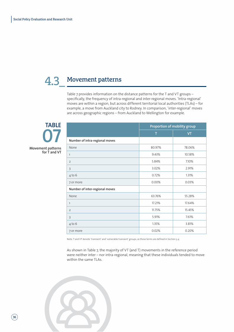
Table 7 provides information on the distance patterns for the T and VT groups – specifically, the frequency of intra-regional and inter-regional moves. ‘Intra-regional’ moves are within a region, but across different territorial local authorities (TLAs) – for example, a move from Auckland city to Rodney. In comparison, ‘inter-regional’ moves are across geographic regions – from Auckland to Wellington for example.

TABLE

07Movement patterns

for T and VT

Proportion of mobility group

T VT

Number of intra-regional moves

None 80.97% 78.06%

1 9.43% 10.58%

2 5.84% 7.10%

3 3.02% 2.91%

4 to 6 0.72% 1.31%

7 or more 0.00% 0.03%

Number of inter-regional moves

None 63.76% 55.28%

1 17.21% 17.64%

2 11.75% 15.45%

3 5.91% 7.61%

4 to 6 1.35% 3.81%

7 or more 0.02% 0.20%

Note: T and VT denote ‘transient’ and ‘vulnerable transient’ groups, as those terms are defined in Section 3.4.

As shown in Table 7, the majority of VT (and T) movements in the reference period were neither inter – nor intra-regional, meaning that these individuals tended to move within the same TLAs.


36

4.4_ Social welfare benefits and services

4.4.1_Associations with social welfare benefit

Data = Benefit dynamicsThe benefit dynamics data in the IDI is provided by the Ministry of Social Development (MSD) and includes information on people who have received a social welfare benefit. This dataset consists of multiple tables that hold details about the primary benefit recipients and also the partners and dependent children included in a benefit, as well as the period for which a person is included in the benefit spell in different roles (that is, as the primary benefit recipient, partner, or dependent child).

Variables created• Indicator for being associated with a social welfare benefit spell (as the primary

benefit recipient; associated partner; associated child; and in general).

• The number of days an individual was associated with the social welfare benefit system.

Time periodPre-reference period = 1 August 2008 to 31 July 2013

Reference period = 1 August 2013 to 31 May 201620

Descriptive analysisFigure 8 presents the proportion of individuals captured by the social welfare benefit system within each of our population subgroups of interest, over the entirety of the pre-reference and reference periods. It shows that 76.3% of those classified as vulnerable transient (VT) were associated with at least one benefit spell either as the primary benefit recipient or as an associated partner or associated dependent child. This is considerably higher than for the other population subgroups. The average for the entire study population is 22.2%.

For those receiving a benefit, Figure 9 shows the proportion of time on a benefit, showing this separately for the pre-reference period and for the reference period.21 Notably, there is no particularly distinct pattern of intensity of use (once an individual has been identified as associated with a benefit) across the subgroups. For instance, the VT group appears to show the same level of intensity of use in the reference period as the Nm group.

20 The benefit dynamics data is only available until 31 May 2016, and therefore we are not able to cover the entire reference period as defined for other datasets.

21 Note that the number of days an individual was involved in the social welfare system is recorded for each role of association (primary benefit recipient, included partner, or dependent child). In cases where an individual was associated with multiple benefits in different roles on the same day, multiple counts of days on benefits will be given to that individual to reflect this additional benefit intensity. Therefore, the role-specific percentage time on benefit, derived from the total number of role-specific days on benefit during a specified time period, could exceed 100%.

37

These results illustrate that frequency of movement alone does not necessarily suggest vulnerability. Those with high movements within low deprivation areas have the second lowest presence in the benefit system and the shortest average length of time on a benefit for those who were on a benefit.

Figure 8 _ Proportion within each population subgroup on benefit

100

80

60

40

20

0

Perc

enta

ge w

ithin

eac

h gr

oup

Population subgroupNm Lm Mm HmU T VT

Associated partner Primary recipient Associated child In any role

(aged under 18)

1.3 2.5 3.8 2.5 4.210.08.0

17.6

27.9

20.2

35.2

58.2

20.6

41.4

54.3

28.7

48.6

73.8

13.9

32.1

45.4

27.6

46.9

76.3

Notes: Data sourced from the IDI benefit dynamics data and matched with the population created from the address table. Timeframe is 1 August 2008 to 31 May 2016. Nm = non-movers; Lm = low movement; Mm = medium movement; HmU = high movement (upward); T = transient; and VT = vulnerable transient (as those terms are defined in Section 3.4).

Figure 9 _ Average time within each population subgroup on benefit

80

60

40

20

0

Aver

age

perc

enta

ge ti

me

on b

enefi

t


Pre-reference period Reference period

50.5%46.9% 47.5%

35.1%39.9%

54.5%

63.1%

57.3% 56.0%

42.4%46.1%

61.7%

Notes: Data sourced from the IDI benefit dynamics data and matched with the population created from the address table. Pre-reference period is 1 August 2008 to 31 July 2013, and reference period is 1 August 2013 to 31 May 2016. Nm = non-movers; Lm = low movement; Mm = medium movement; HmU = high movement (upward); T = transient; and VT = vulnerable transient (as those terms are defined in Section 3.4).


38

4.4.2_Child, Youth and Family events

Data = Child, Youth and Family (CYF)The MSD holds information on Child, Youth and Family intake events, abuse events and placement events, in multiple tables. A child or young person (CYP) is captured in the datasets where:

• a concern is raised about the CYP’s behaviour or insecurity of care

• it is believed that the CYP is being or is likely to be harmed, ill-treated, abused, neglected, or deprived

• it is believed that the CYP is alleged to have committed an offence.

The concern or report is notified to either CYF, the Police (or other enforcement agency), the Youth Court, or the Family Court.

Variables created• Indicator for a CYF event (intake or placement event).

• Number of intake / placement events.


Reference period: 1 August 2013 to 27 July 201622

Descriptive analysisFigure 10 presents the percentage of CYF intake and placement clients in each population subgroup. Among those under 25 years old23 in the VT group, 34.2% were CYF intake clients, which is substantially higher than the 16.2% for the T group and the corresponding figures for the other population subgroups. The figures for placement clients present the same striking differences: for those under 25 years old, 6.6% of the VT group were CYF placement clients, which is nearly triple the equivalent proportion for the T and Mm groups.

For the average CYF client under 25 years of age, those within the VT group incurred, on average, 3.7 events in the pre-reference period and 3.2 events during the reference period. These figures are marginally higher than those for the other population subgroups.

22 The end date is determined by the latest available data.23 CYF social services are for a child or young person (CYP). The CYF characteristics are therefore reported for

populations under 25 years old at the start of our reference period, 1 August 2013, which means under 20 years old at the start of the pre-reference period, 1 August 2008.

39

Figure 10 _ Proportion within each population subgroup that were CYF clients

40

30

20

10

0

Perc

enta

ge w

ithin

eac

h gr

oup


CYF intake clients CYF placement clients

7.9%

16.0%

22.0%

11.0%

16.0%

34.0%

0.5% 1.3% 2.3% 1.2% 2.1%

6.6%

Notes: Data sourced from the CYF data in the IDI and matched with the population created from the address table. Time period = 1 August 2008 to 27 July 2016. Population of interest = age less than 25. Nm = non-movers; Lm = low movement; Mm = medium movement; HmU = high movement (upward); T = transient; and VT = vulnerable transient (as those terms are defined in Section 3.4).

Figure 11 _ Average number of CYF events in each time period, by population subgroups

8

6

4

2

0

Aver

age

inta

ke /

plac

emen

t eve

nts


Intake events in pre-reference period Intake events in reference period Placement events in pre-reference period Placement events in reference period

2.62.9

3.22.7

2.9

3.7

1.92.3

2.6 2.4 2.4

3.2

44.3

4.6

6.2

5.15.5

3

3.7

4.4

5.5 5.65.2

Notes: Data sourced from the CYF data in the IDI and matched with the population created from the address table. Pre-reference period is 1 August 2008 to 31 July 2013, reference period is 1 August 2013 to 27 July 2016. Population of interest = age less than 25. Nm = non-movers; Lm = low movement; Mm = medium movement; HmU = high movement (upward); T = transient; and VT = vulnerable transient (as those terms are defined in Section 3.4).


40

4.4.3_Youth services

Data = Youth servicesThe MSD provides Youth Service intervention (YST) data for integration into the IDI. It contains information about young people participating in different types of youth interventions, including the duration of their participation. The Youth Service targets 15 to 19 year olds who are at risk of long-term benefit dependency; it aims to help young people by moving them into education, training, or work-based learning. We restricted our sample of focus to those aged between 13 and 24 at the start of the reference period (1 August 2013), which accounts for 99.5% of the YST participants matched with our population sample.

Variables created• Indicator of ever participating in a Youth Service.

• If participating in YST, number of days participating.


Reference period = 1 August 2013 to 30 June 201624

Descriptive analysisTable 8 shows both the proportion of youth (aged 13 to 24) receiving YST and, for those who do, the proportion of time spent receiving the service. Once again, those in the VT group stand out: 15.6% of this group received a Youth Service intervention in the pre-reference period, and 14.6% received an intervention in the reference period. Both these statistics are well above the comparable proportions for the other population subgroups of interest.

TABLE

08Youth Service interventions by population

subgroups

Nm Lm Mm HmU T VT

Proportion receiving YST in pre-reference period

2.3% 4.7% 6.7% 3.4% 5.7% 15.6%

Proportion receiving YST in reference period

2.8% 5.2% 6.8% 4.4% 5.8% 14.6%

Average % time on YST in pre-reference period

14.7% 15.0% 15.8% 14.9% 13.8% 15.0%

Average % time on YST in reference period

25.9% 25.7% 26.7% 23.3% 27.3% 30.1%

Notes: Data sourced from the Youth Service interventions tables and matched with the population created from the address table. Pre-reference period is 1 August 2008 to 31 July 2013, reference period is 1 August 2013 to 30 June 2016. Population of interest = age 13 to 24. Average % time on YST is only calculated for users of the service. Nm = non-movers; Lm = low movement; Mm = medium movement; HmU = high movement (upward); T = transient; and VT = vulnerable transient (as those terms are defined in Section 3.4).

24 End date is based on latest available data for youth service interventions.

41

For those who ever participated in any intervention, the amount of time spent on YST is similar across all population subgroups. For instance, the proportion of time on YST in the pre-reference period varied within the small range 13.8% to 15.8%, with the proportion for the VT group (15%) being similar to the proportions for the Lm group (15%) and Mm group (15.5%). A similar pattern is evident for the reference period, although the YST usage frequency is marginally higher for the VT group than for other population subgroups in this timeframe.

4.5_ Housing information

Data = Social housingThis data is provided by Housing New Zealand. It includes information on individuals who are waiting for social housing, and information on those in social housing, along with details of their tenancies.

Variables created• Indicator for whether an individual lived in social housing.

• Number of months a person was in social housing.


Reference period = 1 August 2013 to 31 August 201525

Descriptive analysisAs shown in Figure 12, the vulnerable transient group (VT) had the highest share of its population living in social housing during both periods of interest (16.9% in the pre-reference period, 11.8% in the reference period). In contrast, the HmU group (high movement – upward) had the lowest share of its population living in social housing during both periods of interest (1.3% in the pre-reference period, 0.6% in the reference period).

25 The end date is determined by the latest available data for social housing.


42

Figure 12 _ Proportion within each subgroup living in social housing

20

15

10

5

0

Perc

enta

ge w

ithin

eac

h gr

oup


Pre-reference period Reference period

3.5%

6.0%

8.0%

1.3%

3.1%

16.9%

2.9%

4.6%5.9%

0.6%1.6%

11.8%

Notes: Data sourced from the IDI social housing data and matched with the population created from the address table. Pre-reference period is 1 August 2008 to 31 July 2013, reference period is 1 August 2013 to 31 August 2015. Nm = non-movers; Lm = low movement; Mm = medium movement; HmU = high movement (upward); T = transient; and VT = vulnerable transient (as those terms are defined in Section 3.4).

We also report the average number of months in social housing for individuals who ever lived in social housing26 (see Table 9). Notably, individuals in groups that have high levels of movement (HmU, T and VT) experience lower average numbers of months in social housing than the other population subgroups. For instance, the VT group had the lowest number of months in social housing, in both the pre-reference and the reference period. The inability to secure social housing services for longer could potentially be one of the causes behind high movement.

TABLE

09Average number of

months for social housing users

Periods of interest Nm Lm Mm HmU T VT

Pre-reference period 34.15 27.35 25.09 23.40 22.04 22.62

Reference period 23.92 19.69 17.19 13.61 14.30 13.85

Notes: Data sourced from the social housing tables and matched with the population created from the address table. Pre-reference period is 1 August 2008 to 31 July 2013, reference period is 1 August 2013 to 31 August 2015. Nm = non-movers; Lm = low movement; Mm = medium movement; HmU = high movement (upward); T = transient; and VT = vulnerable transient (as those terms are defined in Section 3.4).

26 This amounts to 185,952 individuals in the pre-reference period, and 144,012 in the reference period.

43

4.6_ Justice events

Data = Court chargesThis dataset incorporates individual-level information on court cases and outcomes provided by the Ministry of Justice. Any individual appearing in this dataset has faced court charges at least once during the time period under study. This dataset documents information on the nature of the offence, the outcome, the sentence type, and the relevant dates for the case (the dates of the offence, hearing, and case outcome). The data is available until 31 December 2013, and therefore our descriptive analysis is restricted to the pre-reference period only.

Variables created• Number of court cases in which an individual was charged.

• Number of cases in which a person was convicted or proven guilty.

• Indicator for whether an individual was imprisoned.

• Maximum offence score of an individual – this is based on the offence score constructed by the Ministry of Justice, which depends on the type of offence, outcome, and sentence assigned to an individual in a court case. The score is positively related to the seriousness of the crime.

Time periodJustice outcomes declared during pre-reference period of 1 August 2008 to 31 July 2013.

Descriptive analysis

Figure 13 _ Proportion within each population subgroup with justice events

25

20

15

10

5

0

Perc

enta

ge w

ithin

eac

h gr

oup


Court cases Convicted/Proven guilty Imprisoned

2.8%

6.8%

10.3%

6.2%

11.0%

25.0%

2.1%

5.3%

8.3%

4.4%

8.4%

21.1%

0.2% 0.6%1.2%

0.4% 1.1%

4.9%

Notes: Data sourced from the IDI court charges table and matched with the population created from the address table. This covers the pre-reference period of 1 August 2008 to 31 July 2013. Nm = non-movers; Lm = low movement; Mm = medium movement; HmU = high movement (upward); T = transient; and VT = vulnerable transient (as those terms are defined in Section 3.4).


44

Figure 13 presents the proportion of each population subgroup who faced court charges, were convicted or proven guilty, and were imprisoned during the pre-reference period. We find that the vulnerable transient group has the highest percentage for all three variables. In particular, a quarter of the VT population had a court case, whereas the proportion for the Nm group was 2.8%. A similar pattern is evident for the likelihood of conviction and imprisonment.

We next focus on those who faced court charges at least once in the pre-reference period.27 These results, presented in Table 10, show that the VT group once again stands out as individuals who were more likely to have experienced negative events in the pre-reference period. They were the group most likely to have had a conviction or been proven guilty, with an average of 5.9 convictions during the five-year timeframe. Additionally, 20.1% of the VT group had 10 or more convictions during that timeframe. Their average offence score was also the highest of all the subgroups, indicating that they were much more likely to be committing serious offences.

TABLE

10Descriptive

information for individuals with

court charges

Characteristics Nm Lm Mm HmU T VT

Having at least one conviction 75.9% 78.0% 80.4% 71.7% 76.2% 85.3%

Average number of convictions 2.4 3.0 3.8 3.3 3.7 5.9

Having ≥ 10 convictions 4.8% 7.2% 10.6% 10.4% 10.4% 20.1%

Maximum offence score ≤ 10 42.0% 38.6% 32.0% 44.7% 35.0% 19.2%

Average maximum offence score 151.1 153.2 178.2 142.8 155.4 233.1

Maximum offence score of ≥100 20.2% 23.8% 29.5% 22.0% 26.9% 42.1%

Notes: Data sourced from the IDI court charges table and matched with the population created from the address table. This covers the pre-reference period of 1 August 2008 to 31 July 2013. Nm = non-movers; Lm = low movement; Mm = medium movement; HmU = high movement (upward); T = transient; and VT = vulnerable transient (as those terms are defined in Section 3.4).

27 This amounts to 193,830 out of the total population sample of 3.86 million.

45

4.7_ Family information

Data = Working for Families (WFF); and life eventsWorking for Families: This is a package aimed at making it easier to work and raise a family. The data is provided by the Ministry for Social Development and includes information on the main components of WFF: these are family tax credits (including family tax credit, in-work tax credit, minimum family tax credit, and parental tax credit), accommodation supplements, and childcare subsidies (including pre-school and out-of-school care subsidies).28 We use monthly information (the lowest level of granularity available) for WFF, sourced from the Lvl_Two_Both_Primary table.

Life events: The Department of Internal Affairs collects information on life events related to births, deaths, marriages, and civil unions registered in New Zealand.

Variables createdWFF:• Indicator of being a WFF recipient.• Average number of dependent children of the WFF recipient.

Life events:• Indicator of getting married / civil union.• Indicator of getting a divorce.

Time periodWFF:Pre-reference period = 1 August 2008 to 31 March 201329

Life event:Pre-reference period = 1 August 2008 to 31 July 2013Reference period = 1 August 2013 to 29 July 201630

Descriptive analysisAs shown in Figure 14, the proportions of T and VT receiving a Working for Families component during the pre-reference period are clearly higher than the comparable proportions for other population subgroups. For instance, just over half of the VT group received WFF in that timeframe, compared to only 16% of individuals in the Nm group (non-movers).

For those observed on WFF,31 we also find that the VT group were more likely to have more than two children, relative to other population subgroups. The proportion of the VT group having more than two children in the pre-reference period was 10.8%.

28 More information can be found at www.workingforfamilies.govt.nz/29 The WFF data is only available until 31 March 2013, and therefore we are not able to cover 100% of the pre-reference

period as defined for other datasets.30 The end date is determined by the latest available data for life events.31 This is 808,668, out of the total population sample of 3.86 million.


46

Figure 14 _ Proportion within each population subgroup receiving working for families

60

50

40

30

20

10

0

Perc

enta

ge w

ithin

eac

h gr

oup


16.4%

26.8% 26.3%

32.3%36.8%

50.4%

Notes: Data sourced from the IDI WFF’s Level_two_both_primary table and matched with the population created from the address table. This covers the period 1 August 2008 to 31 Mar 2013. Nm = non-movers; Lm = low movement; Mm = medium movement; HmU = high movement (upward); T = transient; and VT = vulnerable transient (as those terms are defined in Section 3.4).

Table 11 presents life event information – specifically, information on formal relationship events such as marriages, civil unions, and divorces. Group HmU (high movement – upward) were the most likely to have experienced a marriage or civil union in the pre-reference period; groups Nm and VT were the least likely. A similar pattern holds for likelihood of divorce in the pre-reference period.

Note that there are likely to be many informal relationship events not captured in the IDI, and therefore it is difficult to draw any conclusions from the IDI life event information.

TABLE

11Relationship events for each population

subgroup

% of population subgroup Nm Lm Mm HmU T VT

Marriage / civil union 1.9% 3.8% 3.5% 4.4% 3.9% 2.7%

Divorce 0.7% 1.4% 1.4% 1.9% 1.9% 1.2%

Notes: Data sourced from the life event data in the IDI and matched with the population created from the address table. This covers the pre-reference timeframe of 1 August 2008 to 31 July 2013. Nm = non-movers; Lm = low movement; Mm = medium movement; HmU = high movement (upward); T = transient; and VT = vulnerable transient (as those terms are defined in Section 3.4).

47

4.8_ Health characteristics

Data = Programme for the Integration of Mental Health Data (PRIMHD) National Minimum Dataset (NMDS) National Non-Admitted Patient Collection (NNPAC)These datasets are provided by the Ministry of Health. The PRIMHD collects information on mental health and addiction referrals seen by secondary service providers such as district health boards and non-governmental organisations. The NMDS collects information on publicly funded hospital discharge events. The NNPAC stores data on non-admitted face-to-face secondary care events, such as outpatient and emergency department (ED) visits.

Variables created• Indicator for experiencing a mental health or addiction event, as well as number

of events.

• Indicator for having an acute hospital admission, as well as number of admissions.

• Indicator for having an ED visit, as well as number of visits.


Reference period = starts 1 August 2013; ends 31 December 2014 (PRIMHD), 30 June 2015 (NNPAC), 31 December 2015 (NMDS)

Descriptive analysisAs Table 12 shows, the vulnerable transient (VT) group consistently has the greatest proportion of individuals incurring health events across all three types under consideration, followed by the transient (T) group. The same pattern holds for the number of events the average health user incurred in each of the subgroups. This again confirms the vulnerability of the VT group, as that group is defined in this study.


48

TABLE

12Health events by population

subgroups

Nm Lm Mm HmU T VT

Having an event

Mental health and addiction (MH) 3.6% 8.1% 12.8% 11.6% 17.7% 30.8%

ED visit 29.4% 49.2% 57.5% 56.0% 62.4% 73.7%

Acute admission (AA) 28.3% 45.0% 52.1% 57.6% 59.6% 65.6%

Average number of events

MH in pre-reference period 2.6 2.7 3.1 3.0 3.4 4.5

MH in reference period 2.0 2.0 2.4 2.4 2.6 3.4

ED visits in pre-reference period 2.1 2.3 2.6 2.4 2.8 3.6

ED visits in reference period 1.6 1.7 1.8 1.9 2.0 2.5

AA in pre-reference period 1.8 1.8 1.9 1.9 2.1 2.4

AA in reference period 1.6 1.6 1.7 1.8 1.9 2.1

Notes: Data sourced from the PRIMHD, NMDS, and NNPAC in the IDI and matched with the population created from the address table. Event statistics are for the combined pre-reference and reference periods (dates as indicated above). Nm = non-movers; Lm = low movement; Mm = medium movement; HmU = high movement (upward); T = transient; and VT = vulnerable transient (as those terms are defined in Section 3.4).

4.9_ Case study of Auckland City Mission

Data = Auckland City Mission (ACM)The ACM is an Auckland-based social service provider, which aims to provide services to marginalised and disadvantaged Aucklanders. This includes advocacy, medical services, crisis and community services, homeless services, and social detoxification services.

Variables created• Indicator for use of ACM services (from client table).

• Indicator for drug use (from social detoxification table).

Time periodCombined pre-reference and reference period = 1 August 2008 to 30 April 201632

Descriptive analysisWe focused on the combined time period because of the small size of the Auckland City Mission database relative to the population sample. The ACM client table records information on users of any ACM service. The ACM overwrites each visit made by a client and therefore the data primarily consists of unique records per service user that document the most recent visit. We are therefore unable to identify an individual’s frequency of use of ACM services.

32 The end date is determined by the latest available data for ACM.

49

After linking ACM with the population sample (a match of 12,174 individuals), we first needed to acknowledge (as shown in Table 13) that the proportion of population subgroups who are ACM users is relatively low across the board.33 This is primarily driven by the small size of the ACM dataset (the service is used by a minority of the population). As Table 13 also indicates, the vulnerable transient (VT) group are more likely than other population subgroups to be ACM users.

The Auckland City Mission also operates a social detoxification service that assesses drug use behaviour of those considered to be at risk of having drug-related problems. The detoxification table in the IDI presents details of those who were interviewed and whether these individuals reported using drugs in the past year. As Table 13 shows, within the detoxification sample the VT group were overwhelmingly more likely to have used drugs in the past year, with the likelihood being triple that of the next highest group – that is, 47.8% for VT compared to 16.7% for non-movers (Nm).

TABLE

13ACM characteristics

by population subgroup

Nm Lm Mm HmU T VT

% of population subgroup

ACM user 0.1% 0.3% 0.7% 0.2% 0.5% 2.9%

% of detox sample

Used drugs in the one year prior

16.7% 12.9% 13.9% 0.7% 8.0% 47.8%

Notes: Data sourced from the ACM data in the IDI and matched with the population created from the address table. Information is based on the combined pre-reference and reference periods. Detox sample size = 875. Nm = non-movers; Lm = low movement; Mm = medium movement; HmU = high movement (upward); T = transient; and VT = vulnerable transient (as those terms are defined in Section 3.4).

33 It would be useful to calculate these proportions based on an Auckland sample, rather than for New Zealand. However, inter-regional movements make it difficult to define a constant estimate of our sample from Auckland. Future research could refine these percentages to those who lived in Auckland at least once during the relevant timeframe.


50

05Factors associated with vulnerable transience

51

In Section 4 we outlined a number of datasets from the IDI and used them to characterise the population subgroups of interest. These characteristics were of course purely descriptive, and were in the absence of controlling for other factors. While a number of key factors were identified (such as receiving a benefit), the descriptive statistics didn’t provide strength of association in terms of both magnitude and statistical significance.

Consequently, in this final section we build a logistic regression model to develop odds ratios for the key factors associated with being vulnerable transient (VT).

5.1_ Data

All datasets identified in Section 4 (except for Auckland City Mission – ACM) are utilised in this model. This includes:

• Address table

• Personal details

• Benefit dynamics

• Child, Youth and Family

• Youth service interventions

• Social housing

• Court charges

• Working for Families

• Life events

• PRIMHD

• NMDS

• NNPAC

The address table data permits identification of those belonging to VT (based on the definition in Section 3.4). The binary indicator for being VT is the dependent variable in the analysis that follows. The other datasets provide the explanatory variables, and their definitions are detailed in Table 14. For characteristics, where it is appropriate, we have both an indicator variable, and an interaction term that allows investigation of the marginal impact of additional time / events associated with that characteristic. For example, there are two variables that deal with receiving a benefit, a dummy indicator for being associated with a social welfare benefit, and another variable that involves interaction between that dummy and the number of weeks on the benefit system. This second variable is only relevant for those who experienced benefit association. Similar interactions are generated for CYF and YST events, as well as usage of social housing, court charges, WFF, and all three types of health indicators.

It should also be noted that all explanatory variables (except demographic information) are defined based on information for the pre-reference period, whereas the VT status (our outcome variable) is defined based on information for the reference period. This allows us to investigate the links between characteristics that precede our assigning of VT status.


52

TABL

E

14De

finiti

ons f

or

expl

anat

ory

varia

bles

in lo

gist

ic

regr

essio

n an

alys

is

Char

acte

ristic

sDe

finiti

ons

Dem

ogra

phic

Fem

ale

Age

Ethn

icity

Dum

my v

aria

ble

= 1 i

f fem

ale;

0 o

ther

wise

.Co

ntin

uous

var

iabl

e =

age

in ye

ars.

Dum

my v

aria

bles

for M

āori,

Pas

ifika

, MEL

AA, a

nd O

ther

eth

nici

ty. R

efer

ence

gro

up =

Eur

opea

n.

Bene

fits a

nd so

cial s

ervi

ces

Bene

fitBe

nefit

* nu

mbe

r of w

eeks

CY

FCY

F * n

umbe

r of e

vent

sYS

TYS

T * n

umbe

r of w

eeks

Dum

my v

aria

ble

= 1 i

f ass

ocia

ted

with

ben

efit;

0 ot

herw

iseIn

tera

cted

var

iabl

e =

Bene

fit *

Role

-spe

cific

num

ber o

f wee

ksD

umm

y var

iabl

e =

1 if h

ad a

CYF

inta

ke a

nd/o

r pla

cem

ent e

vent

; 0 o

ther

wise

Inte

ract

ed v

aria

ble

= CY

F * N

umbe

r of C

YF in

take

/pla

cem

ent e

vent

sD

umm

y var

iabl

e =

1 if r

ecei

ved

any y

outh

serv

ice

inte

rven

tions

; 0 o

ther

wise

Inte

ract

ed v

aria

ble

= YS

T * N

umbe

r of w

eeks

par

ticip

atin

g in

YST

Hou

sing

Socia

l hou

sing

Socia

l Hou

sing

* num

ber o

f mon

ths

Dum

my v

aria

ble

= 1 i

f liv

ed in

socia

l hou

sing;

0 o

ther

wise

Inte

ract

ed v

aria

ble

= SH

* N

umbe

r mon

ths i

n so

cial h

ousin

g

Just

ice

Cour

t cha

rges

Co

urt C

harg

es *

num

ber o

f con

vict

ions

Dum

my v

aria

ble

= 1 i

f cha

rged

with

a co

urt c

ase;

0 o

ther

wise

Inte

ract

ed v

aria

ble

= Co

urt C

harg

es *

Num

ber o

f con

vict

ions

Fam

ily

WFF

WFF

* nu

mbe

r of m

onth

sM

arria

ge

Div

orce

Dum

my v

aria

ble

= 1 i

f was

on

WFF

; 0 o

ther

wise

Inte

ract

ed v

aria

ble

= W

FF *

Num

ber o

f mon

ths o

n W

FFD

umm

y var

iabl

e =

1 if g

ot m

arrie

d or

had

civi

l uni

on; 0

oth

erw

iseD

umm

y var

iabl

e =

1 if g

ot d

ivor

ced;

0 o

ther

wise

Hea

lth

Men

tal H

ealth

M

enta

l Hea

lth *

num

ber o

f eve

nts

ED v

isit

ED v

isit *

num

ber o

f day

sAc

ute

adm

issio

nAc

ute

adm

issio

n * n

umbe

r of a

dmiss

ions

Dum

my v

aria

ble

= 1 i

f had

a m

enta

l hea

lth e

vent

; 0 o

ther

wise

Inte

ract

ed v

aria

ble

= M

H *

Num

ber o

f men

tal h

ealth

eve

nts

Dum

my v

aria

ble

= 1 i

f mad

e an

ED

visi

t; 0

othe

rwise

Inte

ract

ed v

aria

ble

= ED

* N

umbe

r of d

ays w

ith E

D v

isits

Dum

my v

aria

ble

= 1 i

f had

an

acut

e ad

miss

ion;

0 o

ther

wise

Inte

ract

ed v

aria

ble

= Ac

ute

adm

issio

n * N

umbe

r of a

cute

hos

pita

l adm

issio

ns

Not

es: D

emog

raph

ic v

aria

bles

are

bas

ed o

n th

e st

art o

f the

refe

renc

e pe

riod

(1 Au

gust

201

3); a

ll ot

her v

aria

bles

are

for t

he p

re-r

efer

ence

per

iod,

as d

etai

led

in S

ectio

n 4.

53

5.2_ Method

We ran three separate models to investigate factors associated with being VT for adults, youth and children separately. Adults are defined as age 20 and over, youth are 15 to 19, and children are under 15 as at the start of the pre-reference period (1 August 2008).

As shown in models 1, 2 and 3 below, the majority of variables are similar across the models. Out of all the possible explanatory variables detailed in Table 14, the adult model (model 1) omits the CYF and YST variables, which are not relevant for adults. The youth model (model 2) omits only the WFF information and relationship event indicators for marriage / civil union and divorce. The child model (model 3) is the same as the youth model, but with court charges and YST information dropped. Court charges are not included as they are not relevant for children, and YST is primarily targeted at 15 to 19 year olds, and therefore outside the age bracket used for model 3.

Model 1:

49

5.2 Method

We ran three separate models to investigate factors associated with being vulnerable transient (VT) for adults, youth and children separately. Adults are defined as age 20 and over, youth are 15 to 19, and children are under 15 as at the start of the pre-reference period (1 August 2008). As shown in models 1, 2 and 3 below, the majority of variables are similar across the models. Out of all the possible explanatory variables detailed in Table 14, the adult model (model 1) omits the CYF and YST variables, which are not relevant for adults. The youth model (model 2) omits only the WFF information and relationship event indicators for marriage / civil union and divorce. The child model (model 3) is the same as the youth model, but with court charges and YST information dropped. Court charges are not included as they are not relevant for children, and YST is primarily targeted at 15 to 19 year olds, and therefore outside the age bracket used for model 3. Model 1:

log𝑃𝑃 𝑉𝑉𝑉𝑉

1 − 𝑃𝑃 𝑉𝑉𝑉𝑉 =

𝛼𝛼! + 𝑋𝑋𝛽𝛽! + 𝛿𝛿!! .𝐵𝐵𝐵𝐵𝐵𝐵𝐵𝐵𝐵𝐵𝐵𝐵𝐵𝐵 + 𝜃𝜃!! . 𝐵𝐵𝐵𝐵𝐵𝐵𝐵𝐵𝐵𝐵𝐵𝐵𝐵𝐵 ×𝑛𝑛𝑛𝑛𝑛𝑛𝑛𝑛𝑛𝑛𝑛𝑛 𝑤𝑤𝑤𝑤𝑤𝑤𝑤𝑤𝑤𝑤 + 𝛿𝛿!! . 𝑆𝑆𝑆𝑆𝑆𝑆𝑆𝑆𝑆𝑆𝑆𝑆𝑆𝑆𝑆𝑆𝑆𝑆𝑆𝑆𝑆𝑆𝑆𝑆𝑆𝑆 + 𝜃𝜃!! . 𝑆𝑆𝑆𝑆𝑆𝑆𝑆𝑆𝑆𝑆𝑆𝑆𝑆𝑆𝑆𝑆𝑆𝑆𝑆𝑆𝑆𝑆𝑆𝑆𝑆𝑆 ×𝑛𝑛𝑛𝑛𝑛𝑛𝑛𝑛𝑛𝑛𝑛𝑛 𝑚𝑚𝑚𝑚𝑚𝑚𝑚𝑚ℎ𝑠𝑠 + 𝛿𝛿!! .𝐶𝐶𝐶𝐶𝐶𝐶𝐶𝐶𝐶𝐶𝐶𝐶ℎ𝑎𝑎𝑎𝑎𝑎𝑎𝑎𝑎𝑎𝑎 + 𝜃𝜃!! . 𝐶𝐶𝐶𝐶𝐶𝐶𝐶𝐶𝐶𝐶𝐶𝐶ℎ𝑎𝑎𝑎𝑎𝑎𝑎𝑎𝑎𝑎𝑎 ×𝑛𝑛𝑛𝑛𝑛𝑛𝑛𝑛𝑛𝑛𝑛𝑛 𝑐𝑐𝑐𝑐𝑐𝑐𝑐𝑐𝑐𝑐𝑐𝑐𝑐𝑐𝑐𝑐𝑐𝑐𝑐𝑐𝑐𝑐 + 𝛿𝛿!! .𝑊𝑊𝑊𝑊𝑊𝑊 + 𝜃𝜃!! . 𝑊𝑊𝑊𝑊𝑊𝑊 ×𝑛𝑛𝑛𝑛𝑛𝑛𝑛𝑛𝑛𝑛𝑛𝑛 𝑚𝑚𝑚𝑚𝑚𝑚𝑚𝑚ℎ𝑠𝑠 + 𝛿𝛿!! .𝑀𝑀𝑀𝑀𝑀𝑀𝑀𝑀𝑖𝑖𝑖𝑖𝑖𝑖𝑖𝑖 + 𝛿𝛿!! .𝐷𝐷𝐷𝐷𝐷𝐷𝐷𝐷𝐷𝐷𝐷𝐷𝐷𝐷 + 𝛿𝛿!! .𝑀𝑀𝑀𝑀𝑀𝑀𝑀𝑀𝑀𝑀𝑀𝑀𝑀𝑀𝑀𝑀𝑀𝑀𝑀𝑀𝑀𝑀ℎ + 𝜃𝜃!! . 𝑀𝑀𝑀𝑀𝑀𝑀𝑀𝑀𝑀𝑀𝑀𝑀𝑀𝑀𝑀𝑀𝑀𝑀𝑀𝑀𝑀𝑀ℎ ×𝑛𝑛𝑛𝑛𝑛𝑛𝑛𝑛𝑛𝑛𝑛𝑛 𝑒𝑒𝑒𝑒𝑒𝑒𝑒𝑒𝑒𝑒𝑒𝑒 + 𝛿𝛿!! .𝐸𝐸𝐸𝐸𝐸𝐸𝐸𝐸𝐸𝐸𝐸𝐸𝐸𝐸 + 𝜃𝜃!! . 𝐸𝐸𝐸𝐸𝐸𝐸𝐸𝐸𝐸𝐸𝐸𝐸𝐸𝐸 ×𝑛𝑛𝑛𝑛𝑛𝑛𝑛𝑛𝑛𝑛𝑛𝑛 𝑑𝑑𝑑𝑑𝑑𝑑𝑠𝑠 + 𝛿𝛿!! .𝐴𝐴𝐴𝐴𝐴𝐴𝐴𝐴𝐴𝐴𝐴𝐴𝐴𝐴𝐴𝐴𝐴𝐴𝐴𝐴𝐴𝐴𝐴𝐴𝐴𝐴𝐴𝐴 + 𝜃𝜃!! . 𝐴𝐴𝐴𝐴𝐴𝐴𝐴𝐴𝐴𝐴𝐴𝐴𝐴𝐴𝐴𝐴𝐴𝐴𝐴𝐴𝐴𝐴𝐴𝐴𝐴𝐴𝐴𝐴 ×𝑛𝑛𝑛𝑛𝑛𝑛𝑛𝑛𝑛𝑛𝑛𝑛 𝑎𝑎𝑎𝑎𝑎𝑎𝑎𝑎𝑎𝑎𝑎𝑎𝑎𝑎𝑎𝑎𝑎𝑎𝑎𝑎

Model 2:



𝛼𝛼! + 𝑋𝑋𝛽𝛽! + 𝛿𝛿!! .𝐵𝐵𝐵𝐵𝐵𝐵𝐵𝐵𝐵𝐵𝐵𝐵𝐵𝐵 + 𝜃𝜃!! . 𝐵𝐵𝐵𝐵𝐵𝐵𝐵𝐵𝐵𝐵𝐵𝐵𝐵𝐵 ×𝑛𝑛𝑛𝑛𝑛𝑛𝑛𝑛𝑛𝑛𝑛𝑛 𝑤𝑤𝑤𝑤𝑤𝑤𝑤𝑤𝑤𝑤 + 𝛿𝛿!! . 𝑆𝑆𝑆𝑆𝑆𝑆𝑆𝑆𝑆𝑆𝑆𝑆𝑆𝑆𝑆𝑆𝑆𝑆𝑆𝑆𝑆𝑆𝑆𝑆𝑆𝑆 + 𝜃𝜃!! . 𝑆𝑆𝑆𝑆𝑆𝑆𝑆𝑆𝑆𝑆𝑆𝑆𝑆𝑆𝑆𝑆𝑆𝑆𝑆𝑆𝑆𝑆𝑆𝑆𝑆𝑆 ×𝑛𝑛𝑛𝑛𝑛𝑛𝑛𝑛𝑛𝑛𝑛𝑛 𝑚𝑚𝑚𝑚𝑚𝑚𝑚𝑚ℎ𝑠𝑠 + 𝛿𝛿!! .𝐶𝐶𝐶𝐶𝐶𝐶𝐶𝐶𝐶𝐶𝐶𝐶ℎ𝑎𝑎𝑎𝑎𝑎𝑎𝑎𝑎𝑎𝑎 + 𝜃𝜃!! . 𝐶𝐶𝐶𝐶𝐶𝐶𝐶𝐶𝐶𝐶𝐶𝐶ℎ𝑎𝑎𝑎𝑎𝑎𝑎𝑎𝑎𝑎𝑎 ×𝑛𝑛𝑛𝑛𝑛𝑛𝑛𝑛𝑛𝑛𝑛𝑛 𝑐𝑐𝑐𝑐𝑐𝑐𝑐𝑐𝑐𝑐𝑐𝑐𝑐𝑐𝑐𝑐𝑐𝑐𝑐𝑐𝑐𝑐 + 𝛿𝛿!! .𝐶𝐶𝐶𝐶𝐶𝐶 + 𝜃𝜃!! . 𝐶𝐶𝐶𝐶𝐶𝐶 ×𝑛𝑛𝑛𝑛𝑛𝑛𝑛𝑛𝑛𝑛𝑛𝑛 𝑒𝑒𝑒𝑒𝑒𝑒𝑒𝑒𝑒𝑒𝑒𝑒 + 𝛿𝛿!! .𝑌𝑌𝑌𝑌𝑌𝑌 + 𝜃𝜃!! . 𝑌𝑌𝑌𝑌𝑌𝑌 × 𝑛𝑛𝑛𝑛𝑛𝑛𝑛𝑛𝑛𝑛𝑛𝑛 𝑤𝑤𝑤𝑤𝑤𝑤𝑤𝑤𝑤𝑤 + 𝛿𝛿!! .𝑀𝑀𝑀𝑀𝑀𝑀𝑀𝑀𝑀𝑀𝑀𝑀𝑀𝑀𝑀𝑀𝑀𝑀𝑀𝑀𝑀𝑀ℎ + 𝜃𝜃!! . 𝑀𝑀𝑀𝑀𝑀𝑀𝑀𝑀𝑀𝑀𝑀𝑀𝑀𝑀𝑀𝑀𝑀𝑀𝑀𝑀𝑀𝑀ℎ ×𝑛𝑛𝑛𝑛𝑛𝑛𝑛𝑛𝑛𝑛𝑛𝑛 𝑒𝑒𝑒𝑒𝑒𝑒𝑒𝑒𝑒𝑒𝑒𝑒 + 𝛿𝛿!! .𝐸𝐸𝐸𝐸𝐸𝐸𝐸𝐸𝐸𝐸𝐸𝐸𝐸𝐸 + 𝜃𝜃!! . 𝐸𝐸𝐸𝐸𝐸𝐸𝐸𝐸𝐸𝐸𝐸𝐸𝐸𝐸 ×𝑛𝑛𝑛𝑛𝑛𝑛𝑛𝑛𝑛𝑛𝑛𝑛 𝑑𝑑𝑑𝑑𝑑𝑑𝑑𝑑 + 𝛿𝛿!! .𝐴𝐴𝐴𝐴𝐴𝐴𝐴𝐴𝐴𝐴𝐴𝐴𝑑𝑑𝑑𝑑𝑑𝑑𝑑𝑑𝑑𝑑𝑑𝑑𝑑𝑑𝑑𝑑 + 𝜃𝜃!! . 𝐴𝐴𝐴𝐴𝐴𝐴𝐴𝐴𝐴𝐴𝐴𝐴𝐴𝐴𝐴𝐴𝐴𝐴𝐴𝐴𝐴𝐴𝐴𝐴𝐴𝐴𝐴𝐴 ×𝑛𝑛𝑛𝑛𝑛𝑛𝑛𝑛𝑛𝑛𝑛𝑛 𝑎𝑎𝑎𝑎𝑎𝑎𝑎𝑎𝑎𝑎𝑎𝑎𝑎𝑎𝑎𝑎𝑎𝑎𝑎𝑎

Model 2:

49

5.2 Method

We ran three separate models to investigate factors associated with being vulnerable transient (VT) for adults, youth and children separately. Adults are defined as age 20 and over, youth are 15 to 19, and children are under 15 as at the start of the pre-reference period (1 August 2008). As shown in models 1, 2 and 3 below, the majority of variables are similar across the models. Out of all the possible explanatory variables detailed in Table 14, the adult model (model 1) omits the CYF and YST variables, which are not relevant for adults. The youth model (model 2) omits only the WFF information and relationship event indicators for marriage / civil union and divorce. The child model (model 3) is the same as the youth model, but with court charges and YST information dropped. Court charges are not included as they are not relevant for children, and YST is primarily targeted at 15 to 19 year olds, and therefore outside the age bracket used for model 3. Model 1:



𝛼𝛼! + 𝑋𝑋𝛽𝛽! + 𝛿𝛿!! .𝐵𝐵𝐵𝐵𝐵𝐵𝐵𝐵𝐵𝐵𝐵𝐵𝐵𝐵 + 𝜃𝜃!! . 𝐵𝐵𝐵𝐵𝐵𝐵𝐵𝐵𝐵𝐵𝐵𝐵𝐵𝐵 ×𝑛𝑛𝑛𝑛𝑛𝑛𝑛𝑛𝑛𝑛𝑛𝑛 𝑤𝑤𝑤𝑤𝑤𝑤𝑤𝑤𝑤𝑤 + 𝛿𝛿!! . 𝑆𝑆𝑆𝑆𝑆𝑆𝑆𝑆𝑆𝑆𝑆𝑆𝑆𝑆𝑆𝑆𝑆𝑆𝑆𝑆𝑆𝑆𝑆𝑆𝑆𝑆 + 𝜃𝜃!! . 𝑆𝑆𝑆𝑆𝑆𝑆𝑆𝑆𝑆𝑆𝑆𝑆𝑆𝑆𝑆𝑆𝑆𝑆𝑆𝑆𝑆𝑆𝑆𝑆𝑆𝑆 ×𝑛𝑛𝑛𝑛𝑛𝑛𝑛𝑛𝑛𝑛𝑛𝑛 𝑚𝑚𝑚𝑚𝑚𝑚𝑚𝑚ℎ𝑠𝑠 + 𝛿𝛿!! .𝐶𝐶𝐶𝐶𝐶𝐶𝐶𝐶𝐶𝐶𝐶𝐶ℎ𝑎𝑎𝑎𝑎𝑎𝑎𝑎𝑎𝑎𝑎 + 𝜃𝜃!! . 𝐶𝐶𝐶𝐶𝐶𝐶𝐶𝐶𝐶𝐶𝐶𝐶ℎ𝑎𝑎𝑎𝑎𝑎𝑎𝑎𝑎𝑎𝑎 ×𝑛𝑛𝑛𝑛𝑛𝑛𝑛𝑛𝑛𝑛𝑛𝑛 𝑐𝑐𝑐𝑐𝑐𝑐𝑐𝑐𝑐𝑐𝑐𝑐𝑐𝑐𝑐𝑐𝑐𝑐𝑐𝑐𝑐𝑐 + 𝛿𝛿!! .𝑊𝑊𝑊𝑊𝑊𝑊 + 𝜃𝜃!! . 𝑊𝑊𝑊𝑊𝑊𝑊 ×𝑛𝑛𝑛𝑛𝑛𝑛𝑛𝑛𝑛𝑛𝑛𝑛 𝑚𝑚𝑚𝑚𝑚𝑚𝑚𝑚ℎ𝑠𝑠 + 𝛿𝛿!! .𝑀𝑀𝑀𝑀𝑀𝑀𝑀𝑀𝑖𝑖𝑖𝑖𝑖𝑖𝑖𝑖 + 𝛿𝛿!! .𝐷𝐷𝐷𝐷𝐷𝐷𝐷𝐷𝐷𝐷𝐷𝐷𝐷𝐷 + 𝛿𝛿!! .𝑀𝑀𝑀𝑀𝑀𝑀𝑀𝑀𝑀𝑀𝑀𝑀𝑀𝑀𝑀𝑀𝑀𝑀𝑀𝑀𝑀𝑀ℎ + 𝜃𝜃!! . 𝑀𝑀𝑀𝑀𝑀𝑀𝑀𝑀𝑀𝑀𝑀𝑀𝑀𝑀𝑀𝑀𝑀𝑀𝑀𝑀𝑀𝑀ℎ ×𝑛𝑛𝑛𝑛𝑛𝑛𝑛𝑛𝑛𝑛𝑛𝑛 𝑒𝑒𝑒𝑒𝑒𝑒𝑒𝑒𝑒𝑒𝑒𝑒 + 𝛿𝛿!! .𝐸𝐸𝐸𝐸𝐸𝐸𝐸𝐸𝐸𝐸𝐸𝐸𝐸𝐸 + 𝜃𝜃!! . 𝐸𝐸𝐸𝐸𝐸𝐸𝐸𝐸𝐸𝐸𝐸𝐸𝐸𝐸 ×𝑛𝑛𝑛𝑛𝑛𝑛𝑛𝑛𝑛𝑛𝑛𝑛 𝑑𝑑𝑑𝑑𝑑𝑑𝑠𝑠 + 𝛿𝛿!! .𝐴𝐴𝐴𝐴𝐴𝐴𝐴𝐴𝐴𝐴𝐴𝐴𝐴𝐴𝐴𝐴𝐴𝐴𝐴𝐴𝐴𝐴𝐴𝐴𝐴𝐴𝐴𝐴 + 𝜃𝜃!! . 𝐴𝐴𝐴𝐴𝐴𝐴𝐴𝐴𝐴𝐴𝐴𝐴𝐴𝐴𝐴𝐴𝐴𝐴𝐴𝐴𝐴𝐴𝐴𝐴𝐴𝐴𝐴𝐴 ×𝑛𝑛𝑛𝑛𝑛𝑛𝑛𝑛𝑛𝑛𝑛𝑛 𝑎𝑎𝑎𝑎𝑎𝑎𝑎𝑎𝑎𝑎𝑎𝑎𝑎𝑎𝑎𝑎𝑎𝑎𝑎𝑎

Model 2:



𝛼𝛼! + 𝑋𝑋𝛽𝛽! + 𝛿𝛿!! .𝐵𝐵𝐵𝐵𝐵𝐵𝐵𝐵𝐵𝐵𝐵𝐵𝐵𝐵 + 𝜃𝜃!! . 𝐵𝐵𝐵𝐵𝐵𝐵𝐵𝐵𝐵𝐵𝐵𝐵𝐵𝐵 ×𝑛𝑛𝑛𝑛𝑛𝑛𝑛𝑛𝑛𝑛𝑛𝑛 𝑤𝑤𝑤𝑤𝑤𝑤𝑤𝑤𝑤𝑤 + 𝛿𝛿!! . 𝑆𝑆𝑆𝑆𝑆𝑆𝑆𝑆𝑆𝑆𝑆𝑆𝑆𝑆𝑆𝑆𝑆𝑆𝑆𝑆𝑆𝑆𝑆𝑆𝑆𝑆 + 𝜃𝜃!! . 𝑆𝑆𝑆𝑆𝑆𝑆𝑆𝑆𝑆𝑆𝑆𝑆𝑆𝑆𝑆𝑆𝑆𝑆𝑆𝑆𝑆𝑆𝑆𝑆𝑆𝑆 ×𝑛𝑛𝑛𝑛𝑛𝑛𝑛𝑛𝑛𝑛𝑛𝑛 𝑚𝑚𝑚𝑚𝑚𝑚𝑚𝑚ℎ𝑠𝑠 + 𝛿𝛿!! .𝐶𝐶𝐶𝐶𝐶𝐶𝐶𝐶𝐶𝐶𝐶𝐶ℎ𝑎𝑎𝑎𝑎𝑎𝑎𝑎𝑎𝑎𝑎 + 𝜃𝜃!! . 𝐶𝐶𝐶𝐶𝐶𝐶𝐶𝐶𝐶𝐶𝐶𝐶ℎ𝑎𝑎𝑎𝑎𝑎𝑎𝑎𝑎𝑎𝑎 ×𝑛𝑛𝑛𝑛𝑛𝑛𝑛𝑛𝑛𝑛𝑛𝑛 𝑐𝑐𝑐𝑐𝑐𝑐𝑐𝑐𝑐𝑐𝑐𝑐𝑐𝑐𝑐𝑐𝑐𝑐𝑐𝑐𝑐𝑐 + 𝛿𝛿!! .𝐶𝐶𝐶𝐶𝐶𝐶 + 𝜃𝜃!! . 𝐶𝐶𝐶𝐶𝐶𝐶 ×𝑛𝑛𝑛𝑛𝑛𝑛𝑛𝑛𝑛𝑛𝑛𝑛 𝑒𝑒𝑒𝑒𝑒𝑒𝑒𝑒𝑒𝑒𝑒𝑒 + 𝛿𝛿!! .𝑌𝑌𝑌𝑌𝑌𝑌 + 𝜃𝜃!! . 𝑌𝑌𝑌𝑌𝑌𝑌 × 𝑛𝑛𝑛𝑛𝑛𝑛𝑛𝑛𝑛𝑛𝑛𝑛 𝑤𝑤𝑤𝑤𝑤𝑤𝑤𝑤𝑤𝑤 + 𝛿𝛿!! .𝑀𝑀𝑀𝑀𝑀𝑀𝑀𝑀𝑀𝑀𝑀𝑀𝑀𝑀𝑀𝑀𝑀𝑀𝑀𝑀𝑀𝑀ℎ + 𝜃𝜃!! . 𝑀𝑀𝑀𝑀𝑀𝑀𝑀𝑀𝑀𝑀𝑀𝑀𝑀𝑀𝑀𝑀𝑀𝑀𝑀𝑀𝑀𝑀ℎ ×𝑛𝑛𝑛𝑛𝑛𝑛𝑛𝑛𝑛𝑛𝑛𝑛 𝑒𝑒𝑒𝑒𝑒𝑒𝑒𝑒𝑒𝑒𝑒𝑒 + 𝛿𝛿!! .𝐸𝐸𝐸𝐸𝐸𝐸𝐸𝐸𝐸𝐸𝐸𝐸𝐸𝐸 + 𝜃𝜃!! . 𝐸𝐸𝐸𝐸𝐸𝐸𝐸𝐸𝐸𝐸𝐸𝐸𝐸𝐸 ×𝑛𝑛𝑛𝑛𝑛𝑛𝑛𝑛𝑛𝑛𝑛𝑛 𝑑𝑑𝑑𝑑𝑑𝑑𝑑𝑑 + 𝛿𝛿!! .𝐴𝐴𝐴𝐴𝐴𝐴𝐴𝐴𝐴𝐴𝐴𝐴𝑑𝑑𝑑𝑑𝑑𝑑𝑑𝑑𝑑𝑑𝑑𝑑𝑑𝑑𝑑𝑑 + 𝜃𝜃!! . 𝐴𝐴𝐴𝐴𝐴𝐴𝐴𝐴𝐴𝐴𝐴𝐴𝐴𝐴𝐴𝐴𝐴𝐴𝐴𝐴𝐴𝐴𝐴𝐴𝐴𝐴𝐴𝐴 ×𝑛𝑛𝑛𝑛𝑛𝑛𝑛𝑛𝑛𝑛𝑛𝑛 𝑎𝑎𝑎𝑎𝑎𝑎𝑎𝑎𝑎𝑎𝑎𝑎𝑎𝑎𝑎𝑎𝑎𝑎𝑎𝑎

Model 3:

50

Model 3:



𝛼𝛼! + 𝑋𝑋𝛽𝛽! + 𝛿𝛿!! .𝐵𝐵𝐵𝐵𝐵𝐵𝐵𝐵𝐵𝐵𝐵𝐵𝐵𝐵 + 𝜃𝜃!! . 𝐵𝐵𝐵𝐵𝐵𝐵𝐵𝐵𝐵𝐵𝐵𝐵𝐵𝐵 ×𝑛𝑛𝑛𝑛𝑛𝑛𝑛𝑛𝑛𝑛𝑛𝑛 𝑤𝑤𝑤𝑤𝑤𝑤𝑤𝑤𝑤𝑤 + 𝛿𝛿!! . 𝑆𝑆𝑆𝑆𝑆𝑆𝑆𝑆𝑆𝑆𝑆𝑆𝑆𝑆𝑆𝑆𝑆𝑆𝑆𝑆𝑆𝑆𝑆𝑆𝑆𝑆 + 𝜃𝜃!! . 𝑆𝑆𝑆𝑆𝑆𝑆𝑆𝑆𝑆𝑆𝑆𝑆𝑆𝑆𝑆𝑆𝑆𝑆𝑆𝑆𝑆𝑆𝑆𝑆𝑆𝑆 ×𝑛𝑛𝑛𝑛𝑛𝑛𝑛𝑛𝑛𝑛𝑛𝑛 𝑚𝑚𝑚𝑚𝑚𝑚𝑚𝑚ℎ𝑠𝑠 + 𝛿𝛿!! .𝐶𝐶𝐶𝐶𝐶𝐶 + 𝜃𝜃!! . 𝐶𝐶𝐶𝐶𝐶𝐶 ×𝑛𝑛𝑛𝑛𝑛𝑛𝑛𝑛𝑛𝑛𝑛𝑛 𝑒𝑒𝑒𝑒𝑒𝑒𝑒𝑒𝑒𝑒𝑒𝑒 + 𝛿𝛿!! .𝑀𝑀𝑀𝑀𝑀𝑀𝑡𝑡𝑡𝑡𝑡𝑡𝑡𝑡𝑡𝑡𝑡𝑡𝑡𝑡𝑡𝑡ℎ + 𝜃𝜃!! . 𝑀𝑀𝑀𝑀𝑀𝑀𝑀𝑀𝑀𝑀𝑀𝑀𝑀𝑀𝑀𝑀𝑀𝑀𝑀𝑀𝑀𝑀ℎ ×𝑛𝑛𝑛𝑛𝑛𝑛𝑛𝑛𝑛𝑛𝑛𝑛 𝑒𝑒𝑒𝑒𝑒𝑒𝑒𝑒𝑒𝑒𝑒𝑒 + 𝛿𝛿!! .𝐸𝐸𝐸𝐸𝐸𝐸𝐸𝐸𝐸𝐸𝐸𝐸𝐸𝐸 + 𝜃𝜃!! . 𝐸𝐸𝐸𝐸𝐸𝐸𝐸𝐸𝐸𝐸𝐸𝐸𝐸𝐸 ×𝑛𝑛𝑛𝑛𝑛𝑛𝑛𝑛𝑛𝑛𝑛𝑛 𝑑𝑑𝑑𝑑𝑑𝑑𝑑𝑑 + 𝛿𝛿!! .𝐴𝐴𝐴𝐴𝐴𝐴𝐴𝐴𝐴𝐴𝐴𝐴𝐴𝐴𝐴𝐴𝐴𝐴𝐴𝐴𝐴𝐴𝐴𝐴𝐴𝐴𝐴𝐴 + 𝜃𝜃!! . 𝐴𝐴𝐴𝐴𝐴𝐴𝐴𝐴𝐴𝐴𝐴𝐴𝐴𝐴𝐴𝐴𝐴𝐴𝐴𝐴𝐴𝐴𝐴𝐴𝐴𝐴𝐴𝐴 ×𝑛𝑛𝑛𝑛𝑛𝑛𝑛𝑛𝑛𝑛𝑛𝑛 𝑎𝑎𝑎𝑎𝑎𝑎𝑎𝑎𝑎𝑎𝑎𝑎𝑎𝑎𝑎𝑎𝑎𝑎𝑎𝑎

Notes: X is a vector of the demographic characteristics. The outcome variable (being VT) is based on the reference period, and all explanatory variables (except for X) are based on the pre-reference period.

Notes: X is a vector of the demographic characteristics. The outcome variable (being VT) is based on the reference period, and all explanatory variables (except for X) are based on the pre-reference period.


54

5.3_ Results

Table 15 presents the results of the logistic regression, where the outcome is belonging to VT. In particular, odds ratios are presented for models 1 through to 3, which provide a measure of association between the set of factors, characteristics or events and the outcome. Odds ratios represent the odds of an outcome occurring given a particular event or characteristic, compared to the odds of the outcome occurring in the absence of that event or characteristic.

To interpret these findings:

Odds greater than 1 reflect a factor that is associated with an increase in likelihood of being VT. For instance, in the equation in the adult model (model 1), female has an odds ratio of 1.246 – this indicates that females are 24.6% more likely to be VT than their male counterparts in the reference period (holding all other factors constant).

Odds below 1 reflect a factor that is associated with a decline in likelihood of being VT. For instance, in the youth model (model 2), Asian has an odds ratio of 0.706. To interpret this, we take the reciprocal (that is, 1/0.706 = 1.416), and this indicates that Asian youth are 41.6% less likely to be VT than the reference group of Europeans (holding all other factors constant).

The asterisks provided next to each odds ratio indicate the statistical significance of the result, with ***, **, and * denoting significance at the 1%, 5%, and 10% levels.

In general, Table 15 shows similar patterns to those revealed in the descriptive statistics presented in Section 4. The key results are summarised below (note that in all interpretations that follow, ceteris paribus holds):34

Ethnicity: the odds of being VT are higher for Māori than for Europeans, regardless of whether we are focusing on the adult, youth or child model. For example, in the adult model, Māori are more than twice as likely to be VT than Europeans, and this difference is significant at the 1% level.35 Pasifika, MELAA, and ‘Other ethnicity’ also show greater odds of being VT than Europeans. Asians are the only ethnic group with lower odds than Europeans – especially in the child model.

34 Note that we also trialled a multinomial logit, with Nm as the base category; and an additional logit model where we compared VT with the most vulnerable Nm’s (defined as those who didn’t move over the sample period and lived in a high deprivation neighbourhood). The results of these additional permutations were qualitatively very similar to the findings provided in Table 14. These additional results are available from the authors on request.

35 As with all information interpreted from this table, it is important to not draw causal links from this logistic analysis.

55

Characteristics Odds ratios (Robust standard errors)

Adults Youth Child

Demographic

Female 1.246*** (0.011) 1.857*** (0.029) 1.693*** (0.028)

Age 0.970*** (0.000) 0.412*** (0.078) 0.695*** (0.008)

Age2 1.000*** (0.000) 1.017*** (0.004) 1.022*** (0.000)

Māori 2.209*** (0.025) 1.674*** (0.032) 1.965*** (0.042)

Pasifika 1.893*** (0.029) 1.247*** (0.031) 1.332*** (0.038)

Asian 0.988 (0.026) 0.706*** (0.030) 0.568*** (0.027)

MELAA 1.526*** (0.024) 1.250*** (0.031) 1.406*** (0.040)

Other ethnicity 1.631*** (0.022) 1.368*** (0.036) 1.452*** (0.052)

Benefits and social services

Benefit 2.671*** (0.038) 2.658*** (0.053) 2.906*** (0.073)

Benefit * number of weeks 1.000*** (0.000) 1.000*** (0.000) 1.000*** (0.000)

CYF - 1.395*** (0.137) 2.387*** (0.125)

CYF * number of events - 0.983*** (0.022) 1.032*** (0.006)

YST - 1.186*** (0.041) -

YST * number of weeks - 1.000*** (0.000) -

Housing

Social housing (SH) 2.221*** (0.052) 1.818*** (0.066) 2.448*** (0.096)

SH * number of months 0.968*** (0.001) 0.979*** (0.001) 0.976*** (0.001)

Justice

Court charges 1.700*** (0.021) 1.560*** (0.030) -

Court Charges * number of convictions 1.030*** (0.002) 1.032*** (0.032) -

Family

WFF 2.049*** (0.053) - -

WFF * number of months 0.999*** (0.000) - -

Marriage / civil union 1.004 (0.020) - -

Divorce 1.226*** (0.033) - -


Adults Youth Child

Health

Mental Health 1.700*** (0.023) 1.431*** (0.034) 1.923*** (0.060)

Mental Health * number of events 1.027*** (0.002) 1.029*** (0.004) 1.066*** (0.010)

ED visit 1.669*** (0.021) 1.618*** (0.032) 1.486*** (0.033)

ED visit * number of days 1.046*** (0.003) 1.075*** (0.005) 1.102*** (0.006)

Acute admission 1.174*** (0.015) 1.111*** (0.025) 1.136*** (0.031)

Acute admission * number of admissions 0.970*** (0.004) 0.938*** (0.008) 0.941*** (0.011)

Number of observations 2,472,243 264,003 405,663

Wald > chi2 151,454.23 31349.24 31,075.56

Pseudo R2 0.241 0.207 0.230

Notes: Reference groups are males, and European. Definitions are provided in Table 14. Adults, youth and children are defined as aged 20+, 15–19, and under 15 at the start of the pre-reference period. The child results are based on a 50% random sample of their population, as their full population model did not converge. The asterisk notations ***, **, and * denote statistical significance at the 1%, 5%, and 10% levels, respectively.

Benefits and social services: If an individual was associated with a benefit in the pre-reference period, their odds of being VT in the reference period is between 2.5 and 3 times greater than for individuals not associated with a benefit spell. Children in particular stand out as most at risk: children associated with a benefit spell are 2.9 times more likely to be VT than those not associated with the benefit system during that pre-reference period. For benefit users, the intensity of the benefit system makes no difference to the odds of being VT. An odds ratio of 1 for the interacted variable ‘Benefit * number of weeks’ indicates that the length of association with the benefit system does not increase or decrease the likelihood of being VT, once the person is already on the benefit system. A similar pattern holds for CYF and YST: experiencing those interventions results in a greater likelihood of being VT, but intensity of involvement does not substantially affect the propensity further.

Housing: Individuals who experienced social housing in the pre-reference period were much more likely to be VT in the reference period. For social housing users, the greater the number of months of social housing, the likelihood of being VT dropped. For example, adults that experienced social housing in the pre-reference period were 121% more likely to be VT in the reference period than adults in the New Zealand population who did not experience social housing in the pre-reference period. Additionally, for those social housing users, an increase in one month of use is equated with a decline of 3.3% in the likelihood of being VT.

Justice: The more court charges incurred in the pre-reference period, the greater the likelihood of being VT in the reference period. This likelihood increases further with each additional charge that results in a conviction.

TABLE

15Logistic regression

results for belonging in the VT group


56


Adults Youth Child

Health

Mental Health 1.700*** (0.023) 1.431*** (0.034) 1.923*** (0.060)

Mental Health * number of events 1.027*** (0.002) 1.029*** (0.004) 1.066*** (0.010)

ED visit 1.669*** (0.021) 1.618*** (0.032) 1.486*** (0.033)

ED visit * number of days 1.046*** (0.003) 1.075*** (0.005) 1.102*** (0.006)

Acute admission 1.174*** (0.015) 1.111*** (0.025) 1.136*** (0.031)

Acute admission * number of admissions 0.970*** (0.004) 0.938*** (0.008) 0.941*** (0.011)

Number of observations 2,472,243 264,003 405,663

Wald > chi2 151,454.23 31349.24 31,075.56

Pseudo R2 0.241 0.207 0.230

Notes: Reference groups are males, and European. Definitions are provided in Table 14. Adults, youth and children are defined as aged 20+, 15–19, and under 15 at the start of the pre-reference period. The child results are based on a 50% random sample of their population, as their full population model did not converge. The asterisk notations ***, **, and * denote statistical significance at the 1%, 5%, and 10% levels, respectively.

Benefits and social services: If an individual was associated with a benefit in the pre-reference period, their odds of being VT in the reference period is between 2.5 and 3 times greater than for individuals not associated with a benefit spell. Children in particular stand out as most at risk: children associated with a benefit spell are 2.9 times more likely to be VT than those not associated with the benefit system during that pre-reference period. For benefit users, the intensity of the benefit system makes no difference to the odds of being VT. An odds ratio of 1 for the interacted variable ‘Benefit * number of weeks’ indicates that the length of association with the benefit system does not increase or decrease the likelihood of being VT, once the person is already on the benefit system. A similar pattern holds for CYF and YST: experiencing those interventions results in a greater likelihood of being VT, but intensity of involvement does not substantially affect the propensity further.

Housing: Individuals who experienced social housing in the pre-reference period were much more likely to be VT in the reference period. For social housing users, the greater the number of months of social housing, the likelihood of being VT dropped. For example, adults that experienced social housing in the pre-reference period were 121% more likely to be VT in the reference period than adults in the New Zealand population who did not experience social housing in the pre-reference period. Additionally, for those social housing users, an increase in one month of use is equated with a decline of 3.3% in the likelihood of being VT.

Justice: The more court charges incurred in the pre-reference period, the greater the likelihood of being VT in the reference period. This likelihood increases further with each additional charge that results in a conviction.

TABLE



TABLE



continued

57

Family: These characteristics were only included in the adult model. We find that being a Working for Families recipient in the pre-reference period is associated with twice the likelihood of being VT in the reference period, relative to those that had no interaction with WFF. Once again, as we also found with benefit spells, increased intensity of service usage is not associated with any increase or decrease in likelihood of being VT. In terms of formal relationship events, marriage / civil union in the pre-reference period is not significantly associated with being VT in the reference period; but having a divorce event is associated with a 22.6% increase in likelihood of being VT, relative to those who didn’t experience a divorce event.

Health: In all three models, having a mental health event in the pre-reference period is associated with a large increase in likelihood of being VT in the reference period. The odds ratio with the largest magnitude is in the child model, where having a mental health event is associated with a 92.3% increased likelihood of being VT, relative to children without that type of health event. Additional events are associated with a 6.6% increased likelihood of being VT for this group. In a similar fashion, emergency department (ED) visits and acute admissions are also associated with an increased likelihood of being VT, with odds ranging from 1.111 to 1.669, depending on which type of health event, and whether we are focusing on adults, youth or children.

Overall: The factors that stand out in all three specifications (adult, youth and child) are being Māori; being associated with a benefit spell; experiencing social housing; having a mental health event; and an ED visit. Additionally, in the adult model, court charges and experiencing WFF also stand out as key factors; both of these had odds ratios of at least 1.7. In addition to the variables mentioned above as relevant to all specifications, for the youth model we find that being female, and having court charges, both have odds ratios in excess of 1.5; and for the child model, being female, and a CYF event, both have odds ratios greater than 1.6.

5.4_ Future research

While the above characteristics have been detailed for the pre-reference period, we cannot infer a causal link between these factors and the status of being VT in the reference period. There is likely to be a complex set of relationships that underpin the associations between these characteristics and being VT. Future research could delve into a number of avenues, including but not limited to the following:

• Identifying major causes of VT and addressing the policy question of what services and programmes, whether existing or new, could help prevent disadvantageous residential movements.

• Predictive risk analysis for services and programmes targeting individuals and their families who are likely to become VT. This would start with modelling the probability of being VT, similar to the risk factor analysis in section 5, followed by an assessment of the accuracy of prediction. The purpose is effective targeting of those most in need of the public services to be provided.


58

• Understanding the welfare impacts for individuals and their families after a period of being VT, as well as the policy question of what services and programmes could help mitigate those negative impacts.36 As this report has shown, this is not going to be an easy task. There will be difficulty in teasing apart the inter-relationships between moving residence and relevant confounding factors, factors that may also relate to the destabilising events that may have caused the movement in the first place.

36 Many thanks to our reviewer, Professor Phil Morrison, for providing both the second and third suggestion for future research avenues.

59

Disclaimer

The results in this report are not official statistics. They have been created for research purposes from the Integrated Data Infrastructure (IDI) managed by Statistics NZ. The opinions, findings, recommendations and conclusions expressed in this report are those of the authors, not Statistics NZ.

Access to the anonymised data used in this study was provided by Statistics NZ in accordance with security and confidentiality provisions of the Statistics Act 1975. Only people authorised by the Statistics Act 1975 are allowed to see data about a particular person, household, business or organisation, and the results in this report have been confidentialised to protect these groups from identification.

Careful consideration has been given to the privacy, security and confidentiality issues associated with using administrative and survey data in the IDI. Further detail can be found in the privacy impact assessment for the Integrated Data Infrastructure, available from www.stats.gov.nz


60

Appendix

Age distribution for each population subgroup

Age-group (in years) Nm Lm Mm HmU T VT

Under 5 7.7% 14.2% 14.9% 11.1% 11.3% 12.9%

6-13 11.5% 12.5% 9.6% 6.2% 5.5% 5.8%

14-17 5.2% 5.6% 6.4% 4.3% 5.3% 9.1%

18-23 6.2% 9.7% 14.6% 12.7% 20.2% 23.7%

24-29 5.6% 9.2% 11.3% 9.8% 14.1% 13.0%

30-39 10.6% 12.6% 12.2% 12.0% 12.5% 12.2%

40-49 14.5% 12.1% 10.7% 13.1% 10.3% 10.1%

50-59 15.6% 10.6% 9.3% 12.8% 9.8% 7.6%

60-69 11.9% 7.8% 6.6% 11.0% 7.0% 3.8%

Above 69 11.2% 5.8% 4.4% 7.1% 4.1% 1.8%

Notes: This table provides the figures behind Figure 6 in the main document. Nm = non-movers; Lm = low movement; Mm = medium movement; HmU = high movement (upward); T = transient; and VT = vulnerable transient (as those terms are defined in Section 3.4). Data sourced from the address table and the personal details tables in the IDI.

Ethnicity distribution for each population subgroup

Ethnicity Nm Lm Mm HmU T VT

European 66.2% 79.9% 79.5% 93.7% 92.0% 72.2%

Māori 15.3% 25.4% 32.5% 14.3% 22.6% 53.9%

Pasifika 9.6% 11.2% 12.5% 4.8% 6.2% 16.4%

Asian 9.5% 8.5% 6.9% 6.2% 5.9% 4.6%

MELAA 7.5% 10.4% 11.2% 12.5% 13.0% 12.0%

Other 6.3% 7.8% 8.3% 8.5% 9.6% 9.7%

Notes: This table provides the figures behind Figure 7 in the main document. Nm = non-movers; Lm = low movement; Mm = medium movement; HmU = high movement (upward); T = transient; and VT = vulnerable transient (as those terms are defined in Section 3.4). Data sourced from the address table and the personal details tables in the IDI.

61

References

Australian Bureau of Statistics. (2012). Australians still on the move. Retrieved from www.abs.gov.au/websitedbs/censushome.nsf/home/CO-68

Bayer, P., Ross, S., & Topa, G. (2005). ‘Place of Work and Place of Residence: Informal Hiring Networks and Labor Market Outcomes,’ Journal of Political Economy, 116 (6): 1150-1196.

Bull, A., & Gilbert, J. (2007). Student movement and schools – what are the issues?. Centre for Research, Evaluation and Social Assessment.

Clark, W., & P. Morrison. (2012). ‘Socio-spatial mobility and residential sorting: Evidence from a large-scale survey’. Urban Studies, 49(15): 3,253-3,270.

Clark, W.A.V. (2016). ‘Life events and moves under duress: Disruption in the life course and mobility outcomes’. Longitudinal and Life Course Studies: International Journal, 7: 218-239.

Champion, T., & Shuttleworth, I. (2015a). Are people moving home less? An analysis of address changing in England and Wales, 1971–2011, using the ONS longitudinal study. London UK Spatial Economics Research Centre, London School of Economics.

Champion, T., & Shuttleworth, I. (2015b). Is internal migration slowing? An analysis of four decades of NHSCR records for England and Wales. UK Spatial Economics Research Centre, London School of Economics.

Cooke, T.J. (2011). ‘It is not just the economy: declining migration and the rise of secular rootedness’. Population, Space and Place, 17: 193-203.

Cooke, T.J. (2013). ‘Internal migration in decline’. The Professional Geographer, 65(4): 664-675.

Currie, J., & Madrian, B.C. (1999). ‘Health, health insurance and the labor market’. Handbook of labor economics, 3: 3,309-3,416.

ERO. (1997). Students at risk: barriers to learning. Education Evaluation Reports, Report No 7. Education Review Office, Wellington.

Exeter, D.J., Sabel, C.E., Hanham, G., Lee, A.C., & Wells, S. (2015). ‘Movers and stayers: The geography of residential mobility and CVD hospitalisations in Auckland, New Zealand’. Social Science and Medicine, 133: 331-339.

Goldstein, S. (1958). Patterns of Mobility, 1910–1950: The Norristown Study. University of Pennsylvania Press, Philadelphia.

Heenan, L.D.B. (1979). ‘Internal migration: inventory and appraisal’. In R.J.W. Neville & C.H. O’Neill (Eds.), The Population of New Zealand. Interdisciplinary perspectives (pp. 60-88). Longman Paul, Auckland.

Heller, T. (1982). ‘The effects of involuntary residential relocation: A review’. American Journal of Community Psychology, 10(4): 471-492.

Hutchings, H.A., Evans, A., Barnes P, Demmler, J., Heaven, M., Hyatt, M.A., James-Ellison, M., Lyons, R.A., Maddocks, A., Paranjothy, S., Rodgers, S.E., & Dunstan, F. (2013). Do children who move home and school frequently have poorer educational outcomes in their early years at school? An anonymised cohort study. PLoS One 8: e70601.

Jelleyman, T., & Spencer, N. (2008). ‘Residential mobility in childhood and health outcomes: a systematic review’. Journal of Epidemiology and Community Health, 62: 584-592.

Johnston, R.J. (1967). ‘A Reconnaissance Study of Population Change in Nidderdale, 1951–1961’. Transactions, Institute of British Geographers, 41: 113–123.

Kariuki, P., Nash, J., & College, M. (1999). ‘The relationship between multiple school transfers during elementary years and student achievement’. Annual Conference of the (American) Mid-South Educational Research Association. Point Clear, AL.


62

Keown, P. (1971) ‘The Career Cycle and the Stepwise Migration Process’. New Zealand Geographer, 27(2): 175-184.

Lupton, R. (2016). ‘Housing policies and their relationship to residential moves for families with young children’. Longitudinal and Life Course Studies: International Journal, 7: 288-301.

Magdol, L. (2002). ‘Is moving gendered? The effects of residential mobility on the psychological well-being of men and women’. Sex Roles, 47(11-12): 553-560.

Molloy, R., Smith, C.L., & Wozniak, A. (2011). ‘Internal migration in the United States’. Journal of Economic Perspectives, 25(2): 1-42.

Morton, S.M.B., Atatoa Carr, P.E., Berry, S.D., Grant, C.C., Bandara, D.K., Mohal, J., & Tricker, P.J. (2014). Growing Up in New Zealand: A longitudinal study of New Zealand children and their families. Residential Mobility Report 1: Moving house in the first 1000 days. Growing Up in New Zealand, Auckland.

Morrison, P.S., & Clark, W.A.V. (2011). ‘Internal migration and employment: macro flows and micro motives’. Environment and Planning A, 43(8): 1,948-1,964.

Morrison, P.S., & Nissen, K. (2010). ‘Moving in and out of areas of deprivation: Evidence from the New Zealand Census’. New Zealand Population Review, 36: 55-80.

Neighbour, M. (2000). Developing an understanding of transient pupils. Te Tai Tokerau Education Centre, Whangarei.

Oishi, S. (2010). ‘The psychology of residential mobility implications for the self, social relationships, and well-being’. Perspectives on Psychological Science, 5(1): 5-21.

Schafft, K.A. (2006). ‘Poverty, residential mobility, and student transiency within a rural New York school district’. Rural Sociology, 71(2): 212-231.

Schwartz, A.E., Stiefel, L. & Cordes, S.A. (2015). Moving Matters: The Causal Effect of Moving Schools on Student Performance. IESP Working Paper 01-15.

Statistics New Zealand. (2001). Population structure and internal migration: 2001 Census. Retrieved from www.stats.govt.nz/Census/2001-census-data/2001-census-population-structure-and-internal-migration.aspx

Statistics New Zealand. (2006). QuickStats About Population Mobility: 2006 Census. Retrieved from www.stats.govt.nz/Census/2006CensusHomePage/QuickStats/quickstats-about-a-subject/population-mobility.aspx

Statistics New Zealand. (2013). Internal migration update. Retrieved from www.stats.govt.nz/browse_for_stats/population/Migration/internal-migration/tables.aspx#internal

Statistics New Zealand. (2017). Information on Integrated Data Infrastructure. Retrieved from www.stats.govt.nz/browse_for_stats/snapshots-of-nz/integrated-data-infrastructure.asp

Stokols, D., Shumaker, S.A., & Martinez, J. (1983). ‘Residential mobility and personal well-being’. Journal of Environmental Psychology, 3(1): 5-19.

Strand S. (2000). Pupil mobility, attainment and progress during key stage one: A case study in caution. Annual Conference of the British Educational Research Association. Cardiff University.

Tunstall, H., Mitchell, R., Pearce, J., & Shortt, N. (2014). ‘The general and mental health of movers to more – and less-disadvantaged socio-economic and physical environments within the UK’. Social Science and Medicine, 118: 97-107.

Weinberg, B.A., Reagan, P.B., & Yankow, J.J. (2004). ‘Do neighborhoods affect hours worked? Evidence from longitudinal data’. Journal of Labor Economics, 22(4): 891-924.

63

The Families Commission operates under the name Social Policy Evaluation and Research Unit (Superu)

Documents

Social Policy Evaluation and Research Unit - AUT · Social Policy Evaluation and Research Unit. ... Population movement during 5 years prior to 2013 ... economic and social science